Prediction of Waste Generation Using Machine Learning: A Regional Study in Korea

Abstract

Accurate forecasting of household waste generation is essential for sustainable urban planning and the development of data-driven environmental policies. Conventional statistical models, while simple and interpretable, often fail to capture the nonlinear and multidimensional relationships inherent in waste production patterns. This study proposes a machine learning-based regression framework utilizing Random Forest and XGBoost algorithms to predict annual household waste generation across four metropolitan regions in South Korea Seoul, Gyeonggi, Incheon, and Jeju over the period from 2000 to 2023. Independent variables include demographic indicators (total population, working-age population, elderly population), economic indicators (Gross Regional Domestic Product), and regional identifiers encoded using One-Hot Encoding. A derived feature, elderly ratio, was introduced to reflect population aging. Model performance was evaluated using R², RMSE, and MAE, with artificial noise added to simulate uncertainty. Random Forest demonstrated superior generalization and robustness to data irregularities, especially in data-scarce regions like Jeju. SHAP-based interpretability analysis revealed total population and GRDP as the most influential features. The findings underscore the importance of incorporating economic indicators in waste forecasting models, as demographic variables alone were insufficient for explaining waste dynamics. This approach provides valuable insights for policymakers and supports the development of adaptive, region-specific strategies for waste reduction and infrastructure investment.

1. Introduction

The acceleration of urbanization, economic expansion, and demographic shifts such as aging populations and evolving household structures have emerged as dominant factors behind the global increase in municipal solid waste generation [1]. According to global projections, nearly 68% of the world’s population will reside in urban areas by 2050, placing tremendous pressure on waste treatment infrastructure and exacerbating issues such as resource depletion, greenhouse gas emissions, and environmental degradation [2]. Ineffective waste management planning can cause significant societal costs and long-term sustainability challenges [3]. Traditionally, linear models such as ARIMA and multiple regression have been widely adopted for waste forecasting due to their interpretability and causal clarity [4]. However, these conventional methods struggle to capture the nonlinear and highly dimensional nature of urban environmental data [5]. Recently, machine learning (ML) has gained prominence for its ability to model complex variable interactions and enhance predictive accuracy [6]. In particular, ensemble algorithms such as Random Forest and XGBoost are recognized for their robustness against data irregularities and ability to quantify feature importance [7,8]. The rise of explainable artificial intelligence (XAI) tools, especially SHAP (Shapley Additive Explanations), has further enabled transparent interpretation of model predictions in environmental applications [9]. Beyond forecasting, ML is also applied in operational aspects of waste management, including route optimization, automated classification, recycling enhancement, and energy recovery [10]. These innovations are increasingly integrated with real-time IoT data streams to develop adaptive and intelligent waste systems. While demographic variables such as population size and household count have traditionally served as primary inputs in waste prediction, recent studies emphasize the importance of incorporating economic and behavioral factors, including industrial activity, tourism volume, aging ratios, and seasonal patterns [11,12].

In aging societies, the share of the elderly population influences consumption patterns and waste composition. In tourism-centric regions, waste generation fluctuates sharply due to seasonal visitor influxes. Recent research during the COVID-19 pandemic showed that policy shocks like social distancing significantly altered household waste behavior, underscoring the need to include dynamic explanatory variables [13]. Furthermore, relying solely on per capita waste metrics may obscure regional differences in economic structure and lifestyle, potentially leading to skewed policy decisions [14]. However, building accurate ML models for waste prediction remains challenging. Issues such as data sparsity, regional imbalance, and insufficient time-series length, especially in areas like Jeju, undermine model generalization. To overcome these limitations, several studies have proposed strategies such as artificial noise injection, cross-validation, regional encoding, and ensemble techniques to improve prediction robustness [15,16,17]. In response, this study proposes a machine learning-based regression framework to forecast annual household waste generation in four metropolitan regions of South Korea: Seoul, Gyeonggi, Incheon, and Jeju. The model leverages demographic and economic variables including derived features such as elderly ratios and incorporates SHAP for interpretability analysis. The framework compares Random Forest and XGBoost performance, offering practical insights for regional waste management and policy design beyond conventional forecasting methods.

Previous studies have demonstrated the utility of machine learning techniques in forecasting waste generation under diverse urban contexts. For instance, Lu et al. (2022) developed a multi-city ML model incorporating regional demographic and socioeconomic features to improve municipal waste prediction accuracy in China [18]. Similarly, Latif et al. (2023) evaluated multiple ML models including Random Forest and XGBoost or household waste prediction in Malaysia and emphasized the importance of local feature relevance in model performance [19]. Kontokosta et al. (2018) further highlighted the necessity of building-level predictors and interpretable outputs to support operational waste management in cities [20]. These studies collectively underscore two key directions: the importance of regional modeling granularity and the need for interpretability in ML-based environmental forecasting. Building on this insight, the present study develops a machine learning-based prediction framework for annual household waste generation in four metropolitan areas of South Korea: Seoul, Gyeonggi, Incheon, and Jeju. To ensure both predictive accuracy and interpretability, Random Forest and XGBoost models are compared, and SHAP analysis is employed to examine variable contributions. This approach aims to capture local socioeconomic dynamics more precisely while providing transparent insights for region-specific policy design. The methodological direction aligns with prior research but is distinguished by its focus on Korean metropolitan contexts, use of population-adjusted unit waste metrics, and in-depth regional model evaluation, including outlier behaviors.

2. Materials and Methods

2.1. Study Area and Variable Description

This study focuses on forecasting municipal solid waste generation in four metropolitan regions in South Korea: Seoul (a densely populated urban form), Gyeonggi (a standard urban form), Incheon (a form with a large floating population), and Jeju (a representative tourist city). Annual data from 2000 to 2023 were collected for analysis. The dependent variable is the total yearly generation (ton/year). Independent variables include PP (total population), YP (working-age population), OP (elderly population), Gross Regional Domestic Product (GRDP), and regional dummy variables to distinguish administrative areas. To capture the degree of aging, a derived variable, elderly ratio (elder_ratio = OP/PP), was also introduced. For machine learning optimization, regional categorical data were transformed using One-Hot Encoding, resulting in four binary variables. All datasets were compiled from public sources, including the Korean Statistical Information Service (KOSIS) [15], the Local Statistical Yearbook published by Statistics Korea [16], and regional GRDP data provided by the Bank of Korea [17]. Variable scaling was applied through normalization to mitigate imbalances in feature magnitude and ensure compatibility with ensemble learning algorithms.

2.2. Prediction Framework Structure

To simulate real-world data noise and enhance generalization ability, Gaussian white noise (mean = 0, σ = 300) was artificially added to a copy of the dependent variable during training. The value of σ = 300 was selected empirically based on preliminary sensitivity analysis, in which various noise levels were tested to evaluate their impact on model stability and performance. Through these tests, σ = 300 was found to strike a desirable balance: it introduced enough perturbation to regularize the learning process and suppress overfitting while preserving the overall structure and temporal trend of the original signal. In particular, this level of noise was effective in preventing the model from over-adapting to idiosyncrasies in regions with limited training data, such as Jeju, where small sample sizes and seasonal fluctuations increase the risk of model instability. The injection of controlled noise also aimed to replicate common anomalies encountered in municipal waste data, such as administrative reporting inconsistencies, spikes from temporary population inflows during tourism seasons, and abrupt changes driven by policy enforcement or external shocks. By exposing the model to these plausible irregularities during training, the robustness of predictions under uncertain conditions was enhanced. This approach is supported by previous research, which has shown that noise injection can serve as a useful regularization technique to improve model generalization, particularly in environmental domains characterized by sparse or heterogeneous data distributions [13].

2.3. Model Configuration and Training

2.3.1. Machine Learning Models and Training Setup

This study employed two ensemble-based regression algorithms, Random Forest Regressor (version 1.6.1) and XGBoost Regressor (version 3.0.0), both of which are well-suited for capturing complex, nonlinear relationships in tabular datasets and offer built-in mechanisms for interpretability and regularization [21]. These tree-based algorithms have been widely adopted in urban environmental modeling due to their strong generalization ability and robustness to feature collinearity [4,5,7]. Random Forest constructs an ensemble of decision trees trained on bootstrap samples, averaging their predictions to reduce variance. This bagging approach offers resilience against overfitting, particularly in datasets where certain variables dominate due to structural bias (e.g., population size). On the other hand, XGBoost utilizes gradient boosting to train trees sequentially, minimizing a specified loss function while employing L1/L2 regularization and shrinkage (learning rate control) for improved convergence and error correction [5]. While other models such as SVR and ANN were considered, they were excluded due to several practical and methodological reasons. SVR, despite its effectiveness in high-dimensional spaces, is sensitive to kernel parameters and less transparent for interpretation. ANNs are typically data-hungry and computationally intensive, and their “black-box” nature undermines their suitability in policy-related applications where interpretability is paramount. In contrast, both Random Forest and XGBoost support SHAP-based interpretability, which allows for the decomposition of predictions into feature-level contributions. This is particularly valuable in environmental domains where stakeholders demand clear explanations for regional differences in forecasted waste volumes. The data were split into training (80%) and testing (20%) subsets. Hyperparameter tuning was conducted using grid search and five-fold cross-validation, as detailed in Section 2.3.1. This process ensured stable performance across folds and minimized overfitting. In addition to training on the original dataset, a second training round was conducted using noise-augmented data to simulate structural shocks and enhance the model’s generalization under uncertainty. To reinforce robustness, multiple evaluation criteria (R², RMSE, MAE, MAPE) were used, and SHAP analysis was applied to the final XGBoost model for global and local interpretation. These components collectively form a comprehensive pipeline suitable for policy-oriented, regionally contextualized waste forecasting.

2.3.2. Hyperparameter Tuning

To optimize model performance while minimizing the risk of overfitting, hyperparameters for both Random Forest and XGBoost were tuned using grid search combined with five-fold cross-validation on the training dataset. This approach enabled a robust estimation of model performance and facilitated the selection of parameter combinations that generalized well across folds [3,22]. For the Random Forest Regressor, the following hyperparameters were tuned based on the prior literature and empirical evaluation [4,7]:

• n_estimators ∈ {100, 300, 500}.
• max_depth ∈ {10, 20, 30, None}.
• min_samples_split ∈ {2, 5, 10}.
• min_samples_leaf ∈ {1, 2, 4}.
• max_features ∈ {“sqrt”, “log2”}.

The final Random Forest model used the configuration

• n_estimators = 300, max_depth = 20, min_samples_split = 5, min_samples_leaf = 2, max_features = “sqrt”, which provided a good trade-off between bias and variance.

For the XGBoost Regressor, the following hyperparameter space was explored, informed by common practice and previous research [5,22]:

• n_estimators ∈ {100, 300, 500}.
• max_depth ∈ {3, 5, 7, 10}.
• learning_rate ∈ {0.01, 0.05, 0.1}.
• subsample ∈ {0.6, 0.8, 1.0}.
• colsample_bytree ∈ {0.6, 0.8, 1.0}.
• gamma ∈ {0, 1, 5}.
• reg_alpha ∈ {0, 0.1, 1}.
• reg_lambda ∈ {1, 5, 10}.

The optimal configuration selected for XGBoost was

• n_estimators = 300, max_depth = 7, learning_rate = 0.05, subsample = 0.8, colsample_bytree = 0.8, gamma = 1, reg_alpha = 0.1, reg_lambda = 5. These settings provided strong predictive accuracy while maintaining generalizability [5]. During tuning, the negative root mean squared error (neg-RMSE) was used as the scoring metric to evaluate performance across folds [3]. All model training and tuning procedures were implemented using the Scikit-learn and XGBoost Python(version 3.12.7) packages. Final models were retrained on the full training set using the optimal hyperparameter configurations before evaluation on the test set. This systematic tuning approach ensured fair model comparison and improved generalization, particularly when tested on administrative units with diverse population sizes and economic conditions [7].

2.4. Evaluation Metrics and Visualization Strategy

To comprehensively assess model performance, we employed four standard regression metrics: the coefficient of determination (R²), root mean squared error (RMSE), mean absolute error (MAE), and mean absolute percentage error (MAPE) [3]. These metrics capture complementary aspects of model accuracy. While R² indicates the proportion of variance explained by the model, RMSE and MAE provide absolute error magnitudes, and MAPE reflects the error relative to actual values, offering a normalized measure of predictive reliability across regions of varying waste generation volumes. To evaluate the model’s generalization ability, we partitioned the dataset into training and testing subsets using an 80/20 split. For each region, we computed R², MAE, RMSE, and MAPE on both subsets to examine consistency in performance and detect potential overfitting. Random Forest and XGBoost models were assessed individually, and their comparative performance is summarized in

Table 1. Model performance comparison on the test dataset.

Model	R2 (95%CI)	RMSE	MAPE (%)
Random Forest	0.9855 [0.9780–0.9987]	500.35	3.88
XGBoost	0.9784 [0.9629–0.9892]	609.84	4.28

, which includes 95% confidence intervals for R² scores computed via bootstrapping with 1000 repeated sampling iterations. This method estimates the variability of R² without assuming any specific distribution and offers a more reliable assessment of model generalization.

The results show that both models achieved high predictive accuracy, with Random Forest yielding slightly lower error metrics and a higher R² compared to XGBoost. This suggests a marginally better generalization capability of the Random Forest model in this application. Nonetheless, both models show strong fit to the data without significant overfitting, as evidenced by consistent performance between training and test sets. To facilitate visual interpretation of prediction accuracy, observed and predicted values were plotted as time series for each administrative region. In addition, yearly prediction errors were illustrated using bar charts to assess temporal sensitivity and detect under- or overestimation patterns [23]. To control for differences in population size, we also computed per capita waste generation values (unit_waste), allowing normalized comparisons across regions [11]. Finally, to improve model interpretability and support actionable insights, we employed SHAP (Shapley Additive Explanations) analysis [6]. SHAP provides a consistent game-theoretic method for attributing a model’s output to individual input features. We applied SHAP specifically to the XGBoost model due to its compatibility with the TreeExplainer algorithm, which enables exact computation of SHAP values in tree-based models. The gradient-boosting framework of XGBoost also facilitates clear decomposition of complex nonlinear feature interactions, making it particularly suited for environmental modeling tasks.

SHAP values were computed on the test set after training completion. The resulting outputs were used to interpret both global and regional feature importances across administrative units. This approach enhances transparency in model decision-making and supports the formulation of targeted waste management policies based on variable influence patterns.

3. Results

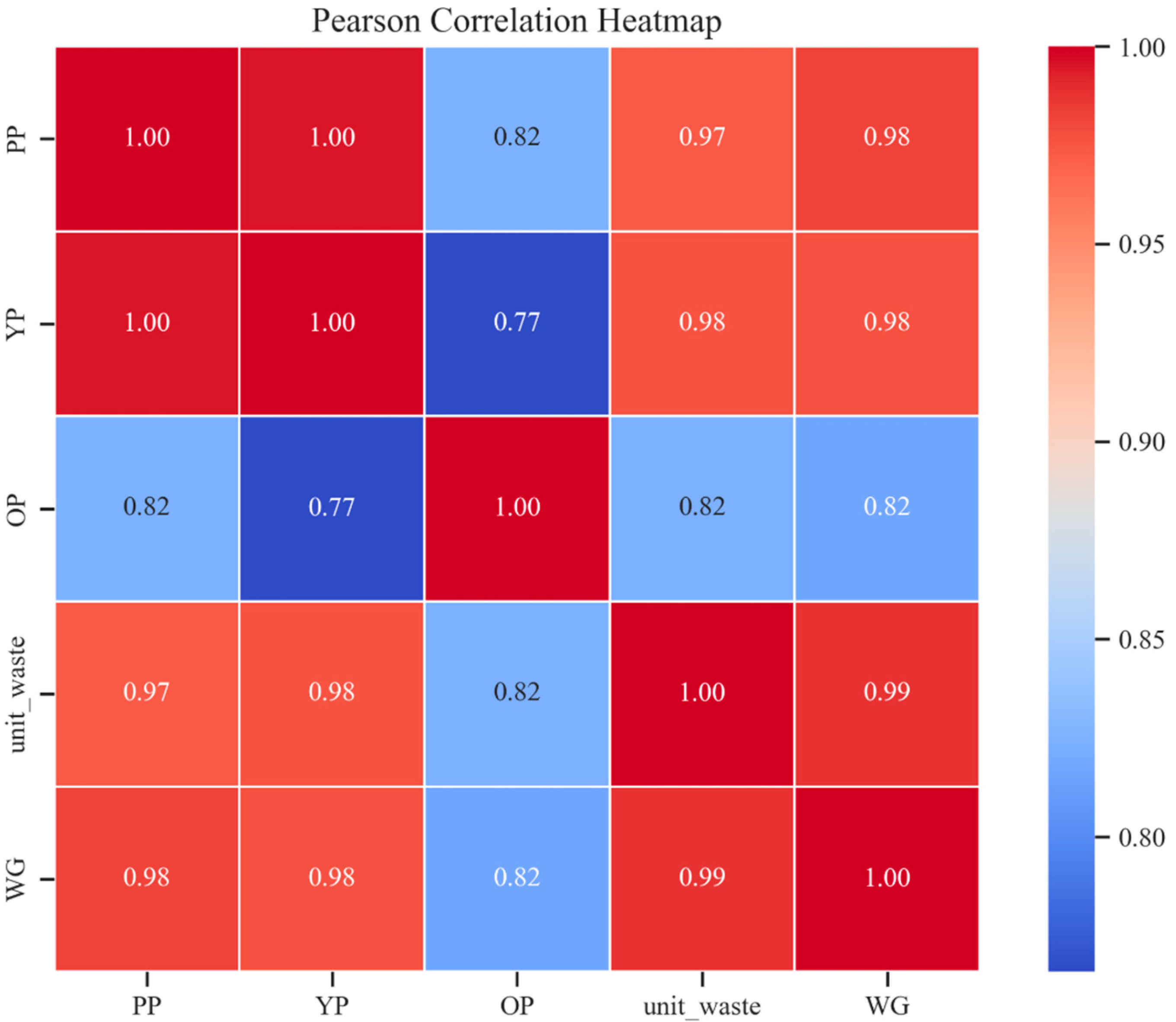
3.1. Correlation Analysis and Feature Interactions

To improve interregional comparability and eliminate population size bias in household waste analysis, this study defines and utilizes a derived feature called unit waste generation (unit_waste). This metric represents per capita household waste, calculated by dividing the total annual household waste by the mid-year population of the corresponding administrative region. The population data were sourced from official government databases including the Korean Statistical Information Service (KOSIS) [15] and the Local Statistical Yearbook [16]. Unit_waste is not an input variable originally included in the raw dataset but a computed ratio that provides insight into the average waste burden per person in each area [11]. The use of this derived indicator is essential because raw waste generation values tend to correlate strongly with population size. Without such normalization, regions with large populations may dominate the data trends, obscuring region-specific behavioral or structural effects. By adjusting for population size, unit_waste reveals intrinsic differences in local waste generation patterns, making it possible to identify regions that produce unusually high or low amounts of waste relative to their population size [19]. This enables more meaningful comparisons in policy and infrastructure evaluation, especially when applying machine learning to multi-regional data.

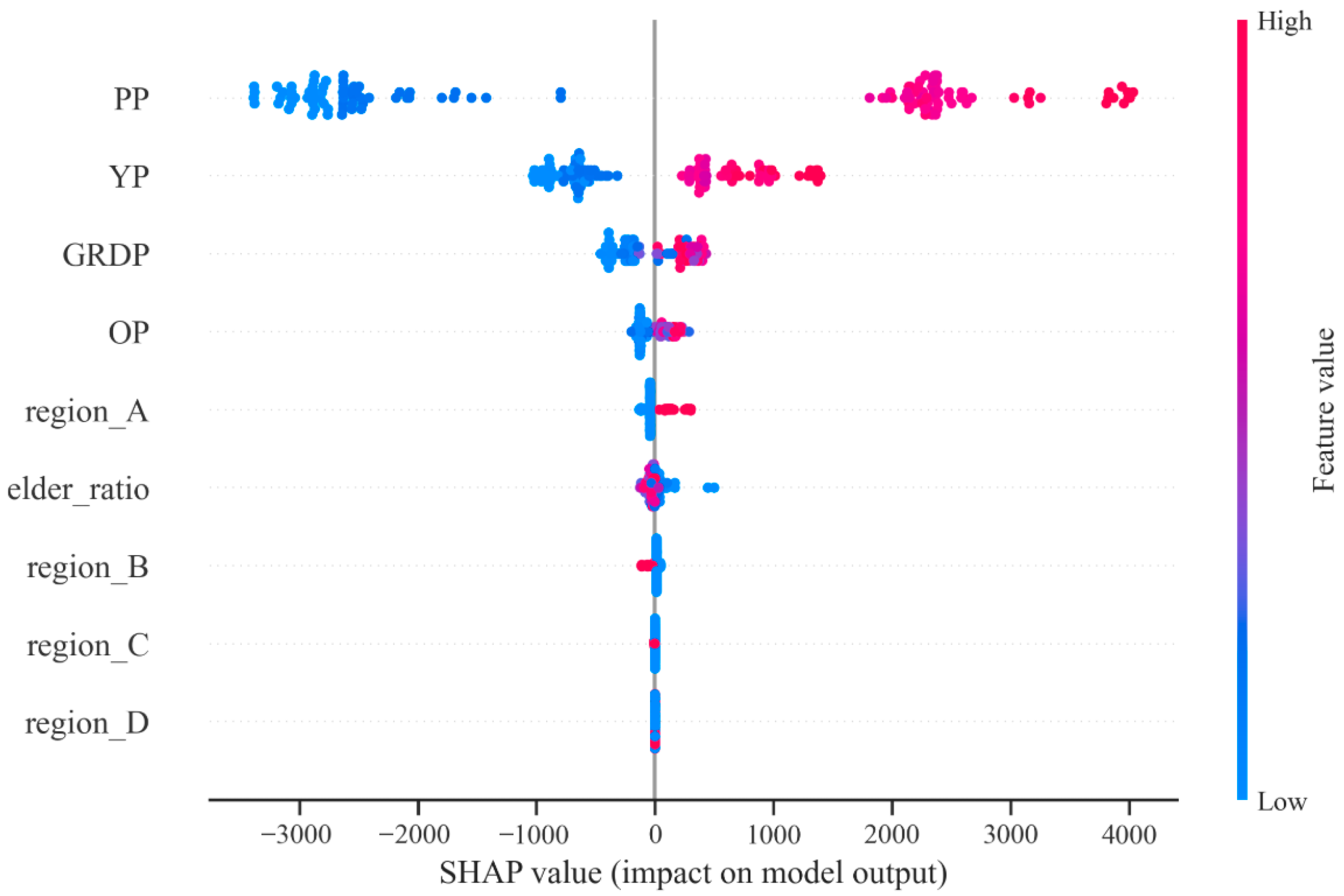
3.2. Feature Importance and Model Interpretation

Figure 1 illustrates the correlation heatmap among the input features, highlighting the strong linear relationship between population and waste generation. Feature importance was explored using SHAP values [6], leveraging the XGBoost model to capture nonlinear interactions and improve interpretability. Figure 2 presents the SHAP summary, where PP and GRDP contributed most substantially to model output. Feature importance was explored using SHAP values [6], leveraging the XGBoost model to capture nonlinear interactions and improve interpretability. Figure 2 presents the SHAP summary, where PP and GRDP contributed most substantially to model output. Figure 2 SHAP summary plot based on the XGBoost model. Feature contributions are ranked across all regions, with total population (PP) and GRDP emerging as the most influential variables. In contrast, elderly population (OP) showed minimal impact, consistent with its weak correlation observed in the data. Interestingly, elderly population (OP) exerted only a minor effect across samples, aligning with its weak statistical correlation observed earlier. Complementing this, Partial Dependence Plots were used to isolate the marginal effect of each input variable on the predicted waste quantity. The PP plot exhibited a near exponential increase, suggesting a nonlinear but strong influence on generation. In contrast, OP and YP showed near-flat responses, confirming their limited explanatory power in this context [6,13]. Figure 3 illustrates the joint distributions and nonlinear relationships among key variables, particularly highlighting the strong association between GRDP and waste generation.

3.3. Regional Forecast Performance

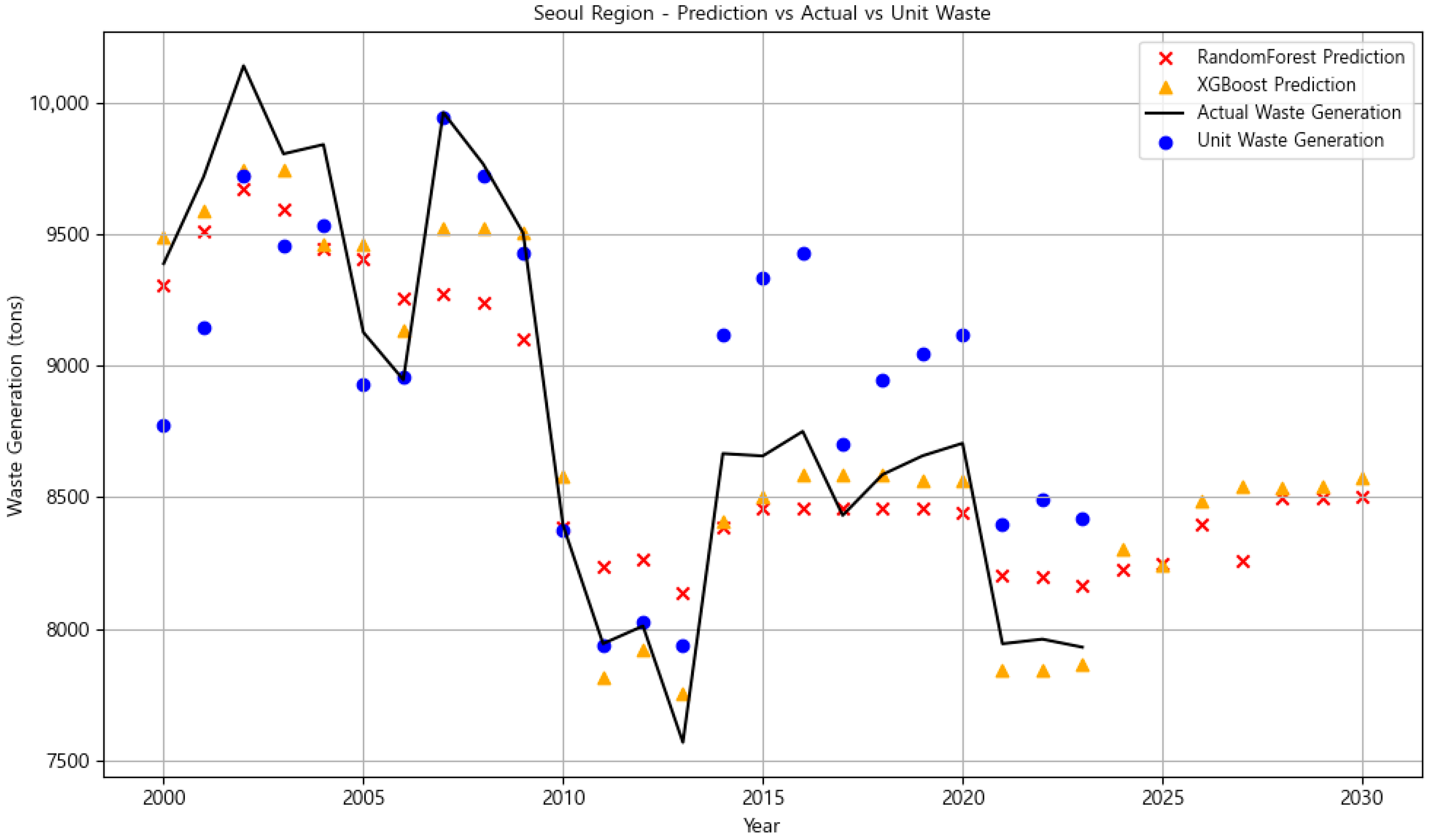
3.3.1. Seoul Region

Among the four metropolitan regions, Seoul exhibited the highest temporal volatility in waste generation. Sharp fluctuations were observed across multiple years, likely driven by a complex interplay of factors such as frequent policy interventions (Figure 4), population dynamics, and high-density urban activities [7,24]. Both models demonstrated reasonable performance in capturing the overall trends. However, XGBoost tended to overfit short-term spikes, particularly after 2015, as it reacted strongly to abrupt changes in the training data [5]. Random Forest, in contrast, maintained a more consistent and stable prediction pattern, but slightly underpredicted during peak waste years [4]. The unit waste generation also showed irregular trends, diverging from the total waste pattern. This divergence highlights a critical modeling challenge: while population-based variables account for broad trends, they fail to capture behavioral or policy-induced shifts that may disproportionately affect per capita waste generation. Incorporating unit waste into the model evaluation revealed that major discrepancies occurred during policy intervention years, suggesting that additional context-sensitive features are required for accurate forecasting in urban regions like Seoul. This suggests that changes in per capita behavior, potentially due to lifestyle shifts, regulatory changes, or public awareness campaigns, may have influenced the waste dynamics [10]. These findings underscore the need to incorporate additional predictors such as floating population, commercial area size, or policy enforcement intensity to improve model performance in high-density urban areas like Seoul [9,25].

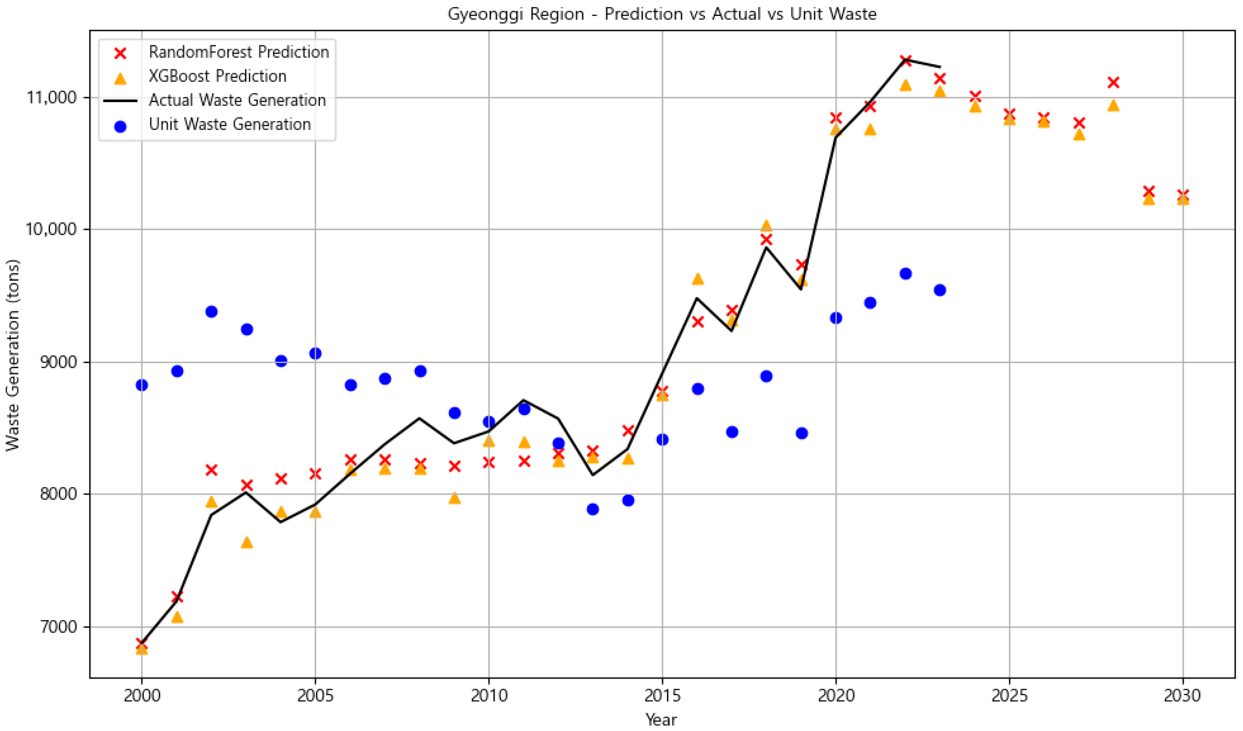
3.3.2. Gyeonggi Region

Gyeonggi Province presented the most stable and linear upward trend in total waste generation among the four regions. Both models performed exceptionally well, with R² values exceeding 0.97 and minimal visual discrepancies between predictions and actual values (Figure 5). The clear upward trend in waste was well captured by both Random Forest and XGBoost, especially after 2015 [26]. Unit waste remained relatively stable over the years, reinforcing the idea that the total increase in waste was mainly driven by population growth rather than changes in per capita behavior [27]. This trend was particularly evident after 2015, where both models showed near-perfect alignment with observed values. The consistent unit waste pattern also implies limited impact from short-term behavioral or policy variations, reinforcing the role of structural drivers such as steady population inflow and housing development. These observations underscore the predictive value of using population-based variables in regions with stable urban growth. Given the region’s continuous urban expansion and strong economic growth, it is likely that the predictive models benefited from a structurally consistent environment with fewer irregular disruptions. This suggests that for regions experiencing steady demographic and economic development, tree-based models can achieve high accuracy. Future studies could further enhance forecasting by including variables such as urban development rates or housing permits as proxies for population influx and built environment expansion [20].

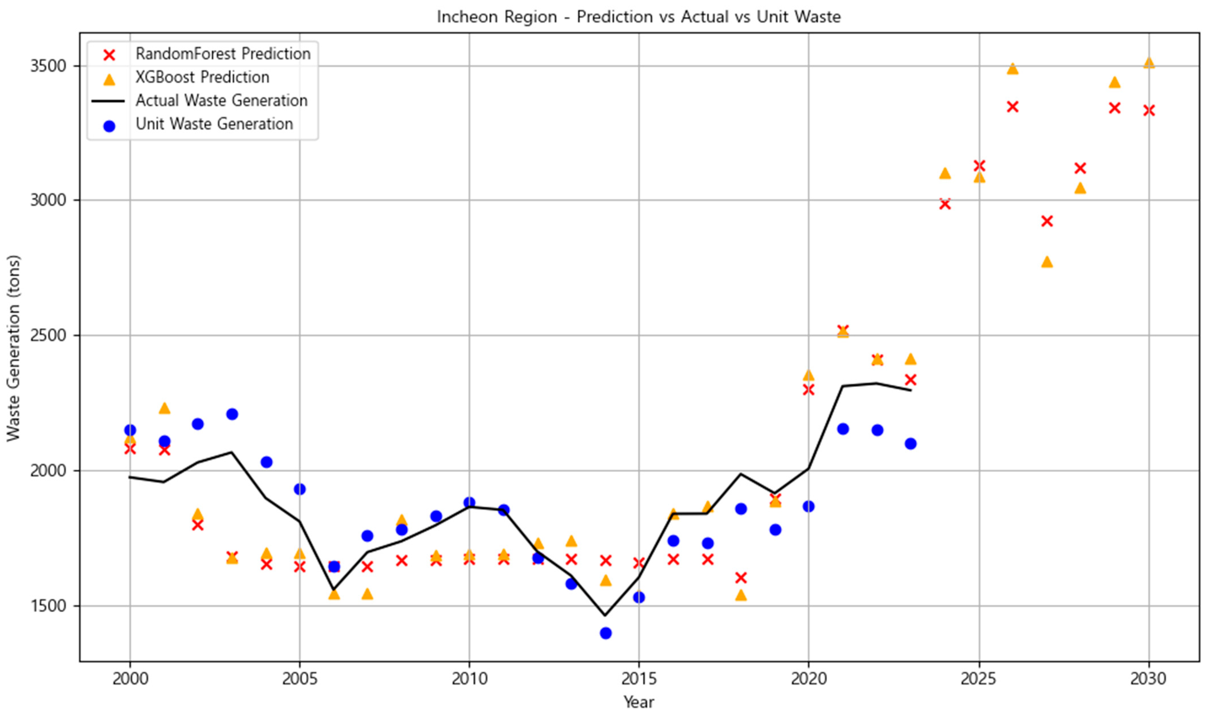
3.3.3. Incheon Region

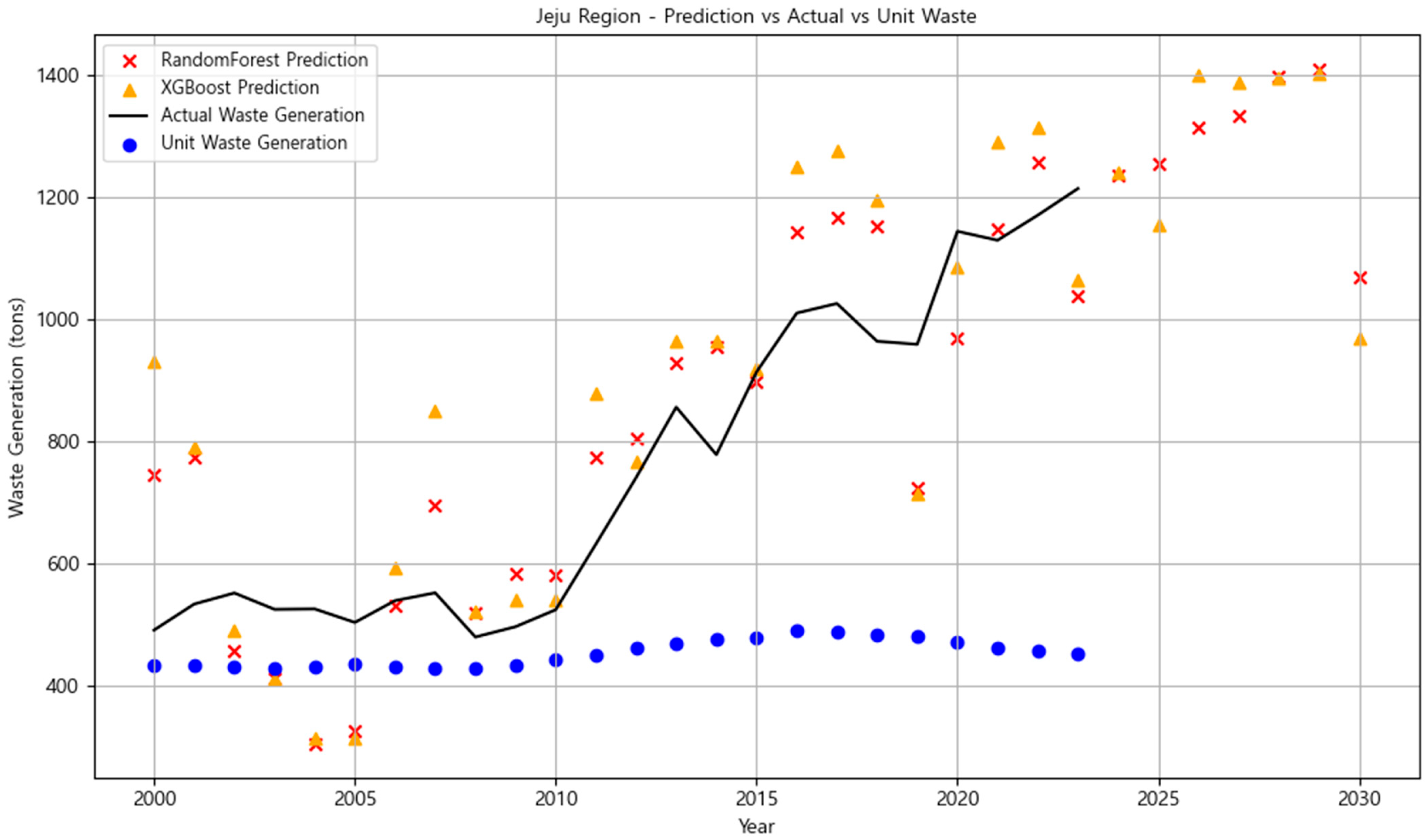
Incheon demonstrated moderate forecasting accuracy, with visible prediction errors in the more recent years. XGBoost frequently overshot actual waste values, especially after 2020, suggesting an over-sensitivity to short-term patterns or nonlinearity in the input features. Random Forest produced relatively closer estimates, although some underprediction was still noted during peak years. Figure 6 shows that unit waste generation fluctuated less than the total waste, indicating that the recent increase in total waste may be largely attributed to external structural drivers such as industrial expansion or changes in household waste behavior. Notably, the forecasting errors in Figure 6 become more pronounced after 2020, particularly for XGBoost, which sharply overshoots observed values in several consecutive years. This suggests a potential model overreaction to recent patterns not present in the historical training data. The relatively smooth unit waste trajectory further implies that transient macro-level factors—rather than household-level behavior—were likely responsible for the observed discrepancies between models and actual waste figures. Additionally, Incheon had relatively sparse or incomplete data in the early 2000s, which may have contributed to reduced generalization during model training. Enhancing prediction accuracy in this region would likely require the inclusion of more detailed industrial, residential, and policy-related variables, as well as improving data quality for earlier time periods [26].

3.3.4. Jeju Region

Jeju Region exhibited relatively stable waste generation patterns throughout the study period, with only minor annual fluctuations. As shown in Figure 7, both Random Forest and XGBoost effectively captured the general upward trajectory of total waste generation. However, a more granular examination of the time series trends reveals that XGBoost consistently underpredicted waste values during peak seasons, particularly between 2017 and 2019. This underestimation may be due to the model’s over-sensitivity to prior averages and inability to capture short-term surges influenced by irregular external events. These discrepancies are clearly observable in Figure 7, where XGBoost predictions consistently fall below actual values during high-demand periods. The years 2017 to 2019, in particular, exhibit the most pronounced underestimations, aligning with known tourism surges. Random Forest, by contrast, tracked these peaks more closely, suggesting greater resilience to short-term external variability. In contrast, Random Forest displayed a more robust performance, maintaining close alignment with actual values during high variance periods, especially between 2015 and 2020. While total waste generation increased, the unit waste generation (waste per capita) remained relatively stable, especially up to 2016, after which a modest rise is observable. This divergence, illustrated in Figure 7, implies that the increase in total waste is not driven by changes in per capita behavior, but rather by structural external factors. The most prominent among these is Jeju’s high seasonal influx of tourists. The discrepancy between unit and total waste trends becomes more visible during summer months, which coincides with the peak tourist season (e.g., July–August), suggesting that transient populations significantly influence overall waste dynamics. Furthermore, Jeju’s insular geography and spatial heterogeneity are not fully captured in standard demographic and economic indicators. Integrating spatial data layers such as land use zones, tourist facility distribution, and road network density can enable more accurate and localized forecasts. The use of Quantum GIS (QGIS) for spatial descriptive and predictive analytics has shown strong potential in identifying inefficiencies, optimizing collection routes, and enhancing site-specific forecasting accuracy. Particularly in environmentally sensitive and logistically constrained regions like Jeju, GIS-supported modeling approaches provide a valuable supplement to traditional machine learning models [27].

3.4. Quantitative Regional Comparison

To supplement the qualitative analyses presented in the preceding sections,

Table 2. Regional model performance with 95% confidence intervals for R².

Region	Model	R2	RMSE	MAPE (%)
Seoul	Random Forest	0.8019 [0.7226–0.8531]	299.48	2.86
	XGBoost	0.9181 [0.8592–0.9486]	192.61	1.70
Gyeonggi	Random Forest	0.9721 [0.9695–0.9846]	217.49	1.95
	XGBoost	0.9752 [0.9540–0.9870]	205.35	1.82
Incheon	Random Forest	0.8934 [0.7676–0.9399]	181.01	7.34
	XGBoost	0.8546 [0.7437–0.9142]	211.39	7.75
Jeju	Random Forest	0.8148 [0.7680–0.8827]	137.60	15.89
	XGBoost	0.6773 [0.4872–0.8091]	181.65	20.02

provide a comprehensive comparison of model performance across four metropolitan regions based on R², RMSE, and MAPE. This multifaceted evaluation is essential, as R² alone is insufficient to fully assess predictive accuracy and model generalizability. Gyeonggi Province recorded the highest predictive performance for both Random Forest and XGBoost, with R² values of 0.9721 and 0.9752 and MAPE values of 1.95% and 1.82%, respectively. The inclusion of 95% confidence intervals further highlights the stability of model predictions in Gyeonggi, as reflected by its narrow R² bounds. In contrast, regions like Incheon and Jeju exhibit wider intervals, indicating greater prediction uncertainty due to data sparsity or structural irregularities. This strong performance likely stems from the region’s consistent population growth and economic development, which provide structurally stable input data. Both models effectively captured nonlinear patterns, consistent with prior studies on ensemble learning in well-structured forecasting tasks [28]. Seoul showed a more nuanced pattern: although XGBoost achieved a higher R² (0.9181 vs. 0.8019) and lower MAPE (1.70% vs. 2.86%) than Random Forest, the gap reflects XGBoost’s sensitivity to short-term fluctuations and potential overfitting under volatile conditions. This corresponds to Zhang et al. (2022), who noted XGBoost’s responsiveness can lead to instability in highly variable time series [29]. In Incheon, both models showed relatively weaker performance. Random Forest and XGBoost yielded R² values of 0.8934 and 0.8546, with corresponding MAPE values of 7.34% and 7.75%. The elevated errors and diminished R² suggest that existing features fail to capture important latent drivers of waste generation in this region such as recent industrial transformation, policy changes, or population mobility. This implies that introducing new features, such as indicators of construction activity or environmental regulations, may be necessary at this stage, rather than postponing to future research. Furthermore, the use of confidence intervals enhances transparency in model evaluation and provides a statistical basis for comparing generalization performance across heterogeneous regions. As Guo et al. (2022) emphasized, integrating such socioeconomic or infrastructural variables can substantially enhance model performance in evolving urban contexts [30]. Jeju remains the most challenging region for both models, with Random Forest (R² = 0.8148, MAPE = 15.89%) outperforming XGBoost (R² = 0.6773, MAPE = 20.02%). These results reflect the region’s irregular waste patterns, influenced by seasonal tourism, sparse early data, and population volatility. Consistent with findings by Hoy et al. (2022), machine learning models applied to small or island regions may struggle with generalizability unless supported by spatial–temporal enhancements [31].

In conclusion, while XGBoost often outperforms in terms of R², its sensitivity may limit its reliability in volatile environments. Random Forest, though occasionally less precise, provides more robust and stable predictions. Crucially, the observed limitations, especially in Incheon, indicate that extending the feature space is not only a direction for future research but an immediate need for improving model accuracy in underperforming regions.

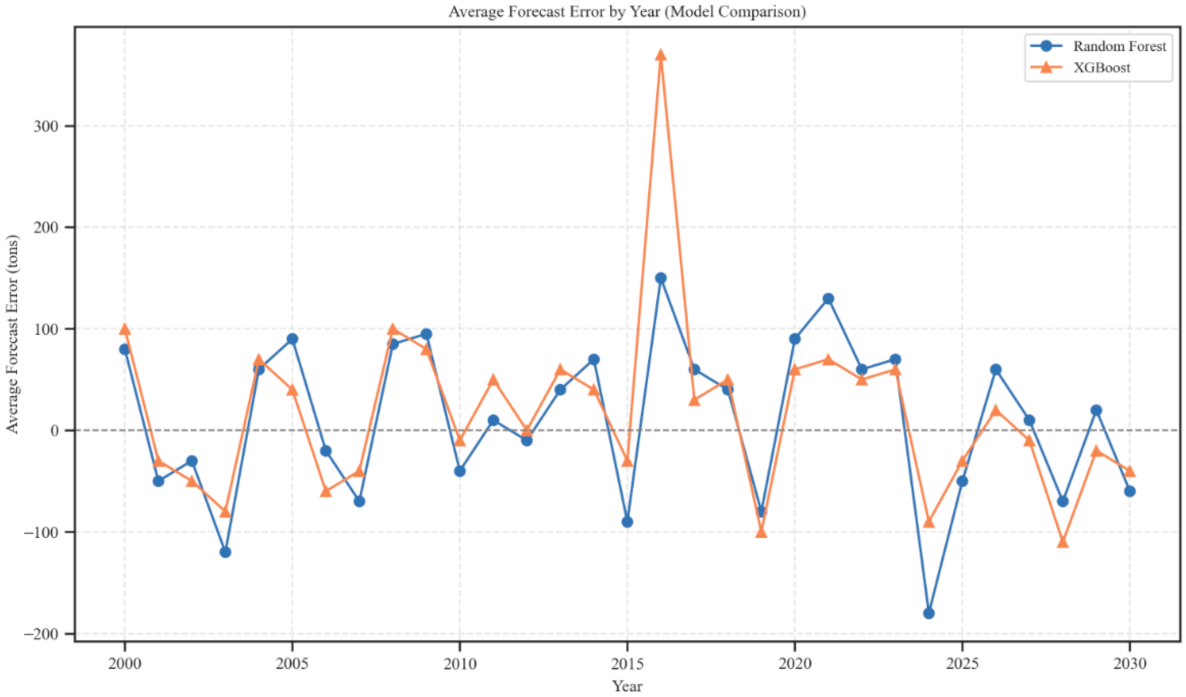
3.5. Temporal Forecast Errors

To evaluate the temporal robustness of the predictive models, year-wise forecast errors were examined for both Random Forest and XGBoost, as shown in Figure 8. This visual comparison highlights substantial interannual variability in prediction accuracy, especially during years impacted by major external shocks. Notably, large error spikes were observed around 2008 and 2020, coinciding with the global financial crisis and the COVID-19 pandemic, respectively. These anomalies underscore the vulnerability of data-driven models when faced with exogenous, rapidly evolving socioeconomic disruptions not captured in historical training data. The sharp peak in 2015 in XGBoost’s forecast error exceeding 350 tons illustrates the model’s heightened sensitivity to residual fluctuations. This is consistent with findings from comparative machine learning research, which have shown that XGBoost, while powerful, may be prone to overreaction in scenarios involving abrupt, unmodeled change [28]. In contrast, Random Forest showed more stable behavior across these turbulent years, with lower error amplitudes and fewer extreme outliers. This robustness stems from the bagging architecture of Random Forest, which averages predictions across multiple trees, thus reducing variance and mitigating the impact of outliers [9]. Over the entire forecast horizon from 2000 to 2030, Random Forest exhibited lower temporal variance, reflecting greater generalization capacity across diverse conditions. Particularly during the post-2020 period, as waste generation patterns shifted due to prolonged behavioral and economic realignment from the pandemic, XGBoost’s performance became increasingly erratic possibly due to its gradient boosting mechanism, which can overweight recent errors and chase noise [22]. This volatility may diminish its suitability for long-term municipal waste forecasting under uncertain macroeconomic conditions. Moreover, the relatively smooth cyclical behavior of Random Forest indicates its effectiveness in capturing underlying trends while buffering against episodic deviations. For municipal planning purposes, this quality is particularly valuable: consistent yet adaptable forecasting is essential for maintaining service efficiency during both stable and crisis periods. Prior studies on waste system resilience have emphasized that forecast consistency, even with slightly reduced precision, may lead to better resource allocation outcomes over time [32].

In summary, this temporal error analysis confirms that while both models demonstrate utility, Random Forest’s temporal stability provides a strategic advantage in real-world waste management settings. For practitioners and policymakers, this highlights the importance of selecting models not only for their point-in-time accuracy, but also for their ability to remain dependable under irregular, high-impact events a growing concern in the face of climate-related, economic, and social volatility.

4. Conclusions

This study demonstrates that machine learning models, particularly ensemble methods like Random Forest and XGBoost, can effectively predict regional waste generation when supported by appropriate contextual information. While XGBoost often delivered higher accuracy, it was also more vulnerable to overfitting and temporal instability in volatile or data-sparse regions. In contrast, Random Forest offered greater robustness, emphasizing the importance of selecting models based not only on accuracy but also on data characteristics and policy demands. However, the analysis revealed that conventional predictors such as population, GRDP, or household counts alone are insufficient to explain the complex patterns observed in certain regions. For instance, regions exhibiting irregular fluctuations or structural changes could not be adequately captured using traditional inputs. This highlights the need to expand the feature set beyond unit waste generation and standard demographic variables. To address these limitations, we recommend incorporating additional features at the current modeling stage, rather than postponing such improvements to future work. These include indicators that reflect floating or commuter population, industrial and construction activity, policy enforcement intensity, real estate trends, and seasonal or weather-related variations. Such variables are more aligned with the underlying drivers of waste generation and can improve both the accuracy and interpretability of predictions. Moreover, advanced methodological approaches such as hybrid spatiotemporal models, causal analysis frameworks, and simulation-based policy scenarios should be explored to further enhance the responsiveness and utility of forecasting systems. These improvements will allow for better handling of temporal variability, more transparent decision-making, and greater adaptability in the face of evolving urban conditions. In conclusion, this study advocates for a paradigm shift in waste prediction practices from static, population-based forecasting toward more comprehensive, economically contextualized, and machine learning-enabled models. Rather than relying solely on population estimates, incorporating a diverse set of contextual indicators can significantly improve predictive performance and provide a more reliable foundation for sustainable and data-driven waste management planning. Furthermore, to improve generalizability across diverse urban contexts, future work should incorporate unmodeled drivers such as tourism volume, industrial activity, and spatial characteristics. Expanding data integration in these directions will help address contextual biases and enhance predictive robustness in both domestic and international applications.

References

1. Kaza, S.; Yao, L.; Bhada-Tata, P.; Van Woerden, F. What a Waste 2.0: A Global Snapshot of Solid Waste Management to 2050; World Bank: Washington, DC, USA, 2018. [Google Scholar] [CrossRef]
2. Guerrero, L.A.; Maas, G.; Hogland, W. Solid waste management challenges for cities in developing countries. Waste Manag. 2013, 33, 220–232. [Google Scholar] [CrossRef]
3. Schratz, P.; Muenchow, J.; Iturritxa, E.; Richter, J.; Brenning, A. Performance evaluation and hyperparameter tuning of statistical and machine-learning models using spatial data. arXiv 2018, arXiv:1803.11266. [Google Scholar] [CrossRef]
4. Breiman, L. Random forests. Mach. Learn. 2001, 45, 5–32. [Google Scholar] [CrossRef]
5. Tasic, A.; Jovanovic, L.; Bacanin, N.; Zivkovic, M.; Simic, V.; Popovic, M.; Antonijevic, M. Towards sustainable so-cieties: Convolutional neural networks optimized by modified crayfish optimization algorithm aided by AdaBoost and XGBoost for waste classification tasks. Appl. Soft Comput. 2025, 175, 113086. [Google Scholar] [CrossRef]
6. Ranjbaran, G.; Recupero, D.R.; Roy, C.K.; Schneider, K.A. C-SHAP: A hybrid method for fast and efficient interpretability. Appl. Sci. 2025, 15, 672. [Google Scholar] [CrossRef]
7. Fang, B.; Yu, J.; Chen, Z.; Osman, A.I.; Farghali, M.; Ihara, I.; Hamza, E.H.; Rooney, D.W.; Yap, P.-S. Artificial intelligence for waste management in smart cities: A review. Environ. Chem. Lett. 2023, 21, 1959–1989. [Google Scholar] [CrossRef]
8. Kumar, R.; Verma, A.; Shome, A.; Sinha, R.; Sinha, S.; Jha, P.K.; Kumar, R.; Kumar, P.; Shubham, S.; Das, S.; et al. Impacts of plastic pollution on ecosystem services, sustainable development goals, and need to focus on circular economy and policy interventions. Sustainability 2021, 13, 9963. [Google Scholar] [CrossRef]
9. Daoud, A.O.; Elattar, H.; Abdelatif, G.; Morsy, K.M.; Peters, R.W.; Mostafa, M.K. Implications of the COVID-19 pandemic on the management of municipal solid waste and medical waste: A comparative review of selected countries. Biomass 2024, 4, 555–573. [Google Scholar] [CrossRef]
10. Alsabt, R.; Alkhaldi, W.; Adenle, Y.A.; Alshuwaikhat, H.M. Optimizing Waste Management Strategies Through Artificial Intelligence and Machine Learning An Economic and Environmental Impact Study. Clean. Waste Syst 2024, 8, 100158. [Google Scholar] [CrossRef]
11. Liu, X.; Zhi, W.; Akhundzada, A. Enhancing performance prediction of municipal solid waste generation: A strategic management. Front. Environ. Sci. 2025, 13, 1553121. [Google Scholar] [CrossRef]
12. Mecheri, H.; Benamirouche, I.; Fass, F.; Ziou, D.; Kadri, N. Prediction of rare events in the operation of household equipment using co-evolving time series. arXiv 2023, arXiv:2312.09410. [Google Scholar] [CrossRef]
13. Branco, P.; Torgo, L.; Ribeiro, R. A survey of predictive modelling under imbalanced distributions. arXiv 2015, arXiv:1505.01658. [Google Scholar] [CrossRef]
14. Pohjankukka, J.; Pahikkala, T.; Nevalainen, P.; Heikkonen, J. Estimating the prediction performance of spatial models via spatial k-fold cross validation. arXiv 2020, arXiv:2005.14263. [Google Scholar] [CrossRef]
15. KOSIS (Korean Statistical Information Service). Available online: https://kosis.kr (accessed on 5 January 2023).
16. Local Statistical Yearbook. Statistics Korea. Available online: https://kostat.go.kr (accessed on 5 January 2023).
17. Bank of Korea. Regional Gross Domestic Product Data. Available online: https://bok.or.kr (accessed on 5 January 2023).
18. Lu, W.; Huo, W.; Gulina, H.; Pan, C. Development of machine learning multi-city model for municipal solid waste generation prediction. Front. Environ. Sci. Eng. 2022, 16, 123. [Google Scholar] [CrossRef]
19. Latif, S.D.; Hazrin, N.A.; Younes, M.K.; Ahmed, A.N.; Elshafie, A. Evaluating different machine learning models for predicting municipal solid waste generation: A case study of Malaysia. Environ. Dev. Sustain. 2023, 26, 12489–12512. [Google Scholar] [CrossRef]
20. Kontokosta, C.E.; Hong, B.; Johnson, N.E.; Starobin, D. Using machine learning and small area estimation to predict building-level municipal solid waste generation in cities. Comput. Environ. Urban Syst. 2018, 70, 151–162. [Google Scholar] [CrossRef]
21. Chen, T.; Guestrin, C. XGBoost: A Scalable Tree Boosting System. In Proceedings of the 22nd ACM SIGKDD International Conference on Knowledge Discovery and Data Mining, San Francisco, CA, USA, 13–17 August 2016; pp. 785–794. [Google Scholar] [CrossRef]
22. Bentéjac, C.; Csörgő, A.; Martínez-Muñoz, G. A Comparative Analysis of Gradient Boosting Algorithms. Information 2020, 11, 193. [Google Scholar] [CrossRef]
23. Ibrahim, K.; Savage, D.A.; Schnirel, A.; Intrevado, P.; Interian, Y. ContamiNet: Detecting contamination in municipal solid waste. arXiv 2019, arXiv:1911.04583. [Google Scholar] [CrossRef]
24. Nam, Y.; Eom, Y.-H. Percolation analysis of spatiotemporal distribution of population in Seoul and Helsinki. arXiv 2024, arXiv:2408.08504. [Google Scholar] [CrossRef]
25. Choi, H.; Kim, J.; Yu, D.; Jun, B. Population concentration in high-complexity regions within city during the heat wave. arXiv 2024, arXiv:2407.09795. [Google Scholar] [CrossRef]
26. Mudannayake, O.; Rathnayake, D.; Herath, J.D.; Fernando, D.K.; Fernando, M. Exploring Machine Learning and Deep Learning Approaches for Multi-Step Forecasting in Municipal Solid Waste Generation. IEEE Access 2022, 10, 10. [Google Scholar] [CrossRef]
27. Imran, M.; Ahmad, S.; Kim, D.H. Quantum GIS Based Descriptive and Predictive Data Analysis for Effective Planning of Waste Management. IEEE Access 2020, 8, 123456–123470. [Google Scholar] [CrossRef]
28. Jayaraman, V.; Lakshminarayanan, A.R.; Parthasarathy, S.; Suganthy, A. Forecasting the Municipal Solid Waste Using GSO-XGBoost Model. Intell. Autom. Soft Comput. 2023, 37, 301–320. [Google Scholar] [CrossRef]
29. Zhang, C.; Dong, H.; Geng, Y.; Liang, H.; Liu, X. Machine learning based prediction for China’s municipal solid waste under the shared socioeconomic pathways. J. Environ. Manag. 2022, 312, 114918. [Google Scholar] [CrossRef] [PubMed]
30. Guo, R.; Liu, H.M.; Sun, H.H.; Wang, D.; Yu, H. Forecasting of municipal solid waste generation in China based on an optimized grey multiple regression model. J. Mater. Cycles Waste Manag. 2022, 24, 2314–2327. [Google Scholar] [CrossRef]
31. Hoy, Z.X.; Woon, K.S.; Chin, W.C.; Hashim, H.; Fan, Y.V. Forecasting heterogeneous municipal solid waste generation via Bayesian-optimised neural network with ensemble learning. Comput. Chem. Eng. 2022, 166, 107946. [Google Scholar] [CrossRef]
32. Liu, J.; Hu, M.; Xu, X. The role of prediction stability in municipal infrastructure under uncertainty. Sustain. Cities Soc. 2021, 69, 102829. [Google Scholar] [CrossRef]
Figure 1. Pearson correlation coefficient heatmap visualizing correlations between variables in color and numerical values to analyze correlation patterns.
Urbansci 09 00297 g001
Figure 2. SHAP summary plot based on the XGBoost model showing global feature importance for all regions.
Urbansci 09 00297 g002
Figure 3. Pairplot showing joint distributions and scatter relationships among variables. Patterns of nonlinearity are evident, especially for GRDP and WG (waste generation).
Urbansci 09 00297 g003
Figure 4. Forecast results for Seoul (2000–2030).
Urbansci 09 00297 g004
Figure 5. Forecast results for Gyeonggi (2000–2030).
Urbansci 09 00297 g005
Figure 6. Forecast results for Incheon (2000–2030).
Urbansci 09 00297 g006
Figure 7. Forecast results for Jeju (2000–2030).
Urbansci 09 00297 g007
Figure 8. Year-wise comparison of average forecast errors for Random Forest and XGBoost models. Spikes in 2008 and 2020 reflect the effects of global economic shocks.
Urbansci 09 00297 g008