Deriving Environmental Properties Related to Human Environmental Perception: A Comparison Between Aerial Image Classification and Street View Image Segmentation

Abstract

In recent decades, urban residents’ perceptions of their surrounding environment have been widely studied, especially pertaining to the association between environmental settings and humans’ psychological wellbeing. Many studies have used aerial imagery to derive environmental properties through image classification to approximate humans’ perceived environment, while a growing number of studies use street view imagery to achieve the same with image segmentation. There is limited research comparing the two approaches. This study aims to examine how the environmental properties derived from aerial and street view images correspond with each other. We utilized two study sites in urban communities in New Jersey, United States. High-resolution aerial images were acquired and classified to derive environmental properties within set buffer zones around sample points where Google Street View images were collected for image segmentation to derive corresponding environmental properties. Several buffer sizes were experimented with. The results show that the amount of greenness and individual environmental elements derived from street view versus aerial images can be quite different at the same locations. The amount of trees derived has a greater concordance between aerial and street views than the amount of buildings derived. The amounts of grass and roads are not in agreement between the two views. Trees derived from street view images correspond with those derived from aerial better when using a small, 30 m buffer. Low-rise buildings and grass agree better when using larger buffer sizes such as 60 m and 100 m. Roads correspond better when larger buffers are employed in green environments, but smaller buffers in environments with limited greenness. Our findings indicate that the choice of buffer size used when combining environmental properties derived from both aerial and street view images together should consider both the environmental elements involved and the type of environmental settings.

1. Introduction

As people interact daily with their surrounding environment, their environmental settings can affect their psychological states through active and passive environmental perception [1]. Urban populations have seen a rise in the prevalence of mental health disorders [2]. Among other factors, this is believed to be linked to the perceived disconnection from nature in the expanding built environment [3]. Humans have an innate desire to seek out natural stimuli that evoke an immediate, active, affective response in our brains and neuroendocrine systems [4]. The presence of these natural elements in and around the environments we live in are therefore associated with beneficial mental wellbeing [5,6,7]. An abundance of research has indicated that one major component of nature, greenspace, lowers the risk of psychosocial and psychological stress [2,8,9] as well as stress-related disorders like depression and anxiety [10,11,12,13]. Urban greenspace has also been shown to contribute to residents’ happiness [14]. Greater integration of natural elements such as greenspace into our growing urban environment, therefore, provides a promising solution that promotes mental health for urban dwellers worldwide [15,16].

Much of the previous research on urban environmental perception and mental health has used aerial imagery to quantify environmental properties. For example, the Normalized Differential Vegetation Index (NDVI), derived from aerial imagery, has been popularly used to quantify environmental properties pertaining to greenspace [17,18,19,20,21,22,23,24]. The spatial resolution of the aerial imageries used ranges from 0.5 m to 30 m [17,18,21,24,25,26]. A resolution of 30 m has been found effective in categorizing greenness on a national scale when studying its impact on depression and anxiety [18]. With a fine resolution of 0.5 m, micro-scale studies have been conducted to investigate the dynamic environmental settings pertaining to individuals’ environmental perceptions and psychological states [27,28]. When correlating the attributes of mental wellbeing with the prevalence of greenspace, these studies used buffer zones around either postal code addresses or individuals’ whereabouts [21,27,28,29]. Most studies identified positive associations between the amount of greenspace and the presence of attributes of positive mental wellbeing, regardless of the choice of buffer size [21,28].

There has also been an increasing trend in utilizing street view imageries to measure the level of greenery at eye level in recent years. A variety of street view imageries, including Google Street View (GSV), Tencent Online Map (TOM), and Baidu maps (BM) databases [17,19,22,23,24,26], have been used to derive environmental elements through image segmentation. Studies have commonly calculated a Green View Index (GVI), Panoramic View Green Index (PVGI), or Blue View Index (BVI), or a combination of these. The environmental elements segmented from street view images vary but often include vegetation, grass, trees, water, buildings, roads, and sky [30,31,32,33], from which the indices are calculated. Studies have shown that individuals’ emotional states lean more positively toward a street landscape when the GVI is above a certain threshold [19,30,32,33,34]. The level of greenery derived from street view images, however, is found to be affected by factors such as image segmentation methods and data collection seasons [31,32]. Results relating to the impact of identifiable greenspace on individuals’ mental wellbeing were also inconsistent. Some studies identified a strong positive correlation between a high GVI and BVI, and good mental wellbeing [17,23,24,25]. Other studies only found correlations between a high GVI and BVI, and a lack of negative effects [18,19,20,22,35].

Several studies have sought to utilize both aerial and street view imagery to identify environmental elements as related to mental wellbeing. For example, one study derived NDVI from aerial imagery within a 1 km buffer of the centroid of the dissemination area, while deriving GVI from GSV to measure the active living environment of Ottawa [22]. The study evaluated the two sets of environmental properties separately. It found that NDVI was not associated with participation in recreational activities by residents, while GVI was positively associated with participation in recreational activities during the summer. Another study incorporated NDVI derived from aerial imageries and GVI derived from Baidu Maps on several Chinese university campuses [24] to study the correlation between greenspace exposure and mental health. Its results demonstrate a negative correlation between greenspace exposure on campuses and the level of mental health issues among university students. A third study derived NDVI from aerial imagery within a 50 m buffer of the GSV latitude/longitude coordinates, while deriving GVI from GSV to create a GVI/NDVI ratio to capture the vertical dimension of greenspace [23]. This study found that utilizing both NDVI and GVI captures more characteristics of the street view greenspace environment than assessments based solely on either single measure [23].

There is a consistent agreement that aerial and street view imagery capture different aspects of the urban environment’s properties [18,22,23,24] and that a combination of both may offer a more comprehensive characterization of humans’ perception of the environment [23]. Such combination, however, is challenged by the inconsistency of the correlations between environmental properties derived from aerial and street view images found in the different studies. For example, there are conflicting results from studies in Amsterdam [18], Beijing [36], and Singapore [37] when correlating the GVIs derived from aerial and street view images. The buffer sizes applied on aerial images are also found to play inconsistent roles in these studies [18].

At the same time, studies examining the associations between mental health and environmental perception continue to grow rapidly, and the most popular approach is still utilizing either aerial or street view images. Among the most recent studies, aerial images have been used to either capture people’s dynamic activity space at the micro-scale [28] or to catalog urban greenspace at a large scale to develop a comprehensive typology representing various environmental settings [38,39]. Street view images, on the other hand, have been used to capture residents’ perceived environments at sampling locations where such images are available in various cities around the world [40,41,42,43]. In other words, aerial images have the advantage of capturing environments with no fixed viewing points and also doing so at a large scale, while street view images provide environmental characterizations in a sampled manner because they cannot cover the entire study area.

In summary, there has been an abundance of studies examining the relationships between urban environmental perception and people’s psychological wellbeing, and valuable findings have been made both evidentially and theoretically. Imageries, both aerial and street view, have been used as data essential for quantifying environmental properties. We recognize several common issues when reviewing these previous studies. First, the prevalent use of NDVI or GVI compounds all forms of greenspace into a single measurable number that does not account for specific environmental elements working as visual stimuli triggering psychological responses [18,19,44]. According to prevalent theories on the mechanisms of how the environment affects our psychological responses [4,45,46], it is the specific visual stimuli in the environment and not the overall greenness that have either a restorative effect or trigger active affect and functions in the pathway to stress reduction, promoting happiness and positive mental health. It is thus necessary to capture the specific visual elements in environments when examining their relation to mental health. Secondly, most studies have only focused on greenspace and the natural elements in the environment. There is a shortage of studies examining the impact of negative environmental stimuli and artificial environmental elements such as buildings and cars, among others. Thirdly, when using aerial imagery to derive environmental properties, there is still the question of what buffer size provides the most information on how an individual is affected by their environment [22,29,30,47]. And lastly, as aforementioned, there has been an increasing use of street view images in recent years, as they capture environmental properties at eye level and thus are believed to directly reflect people’s perceived environment. This implies its advantages over aerial images, which do not directly reflect how humans perceive their surrounding environment. The disadvantage, however, is that street view images do not fully cover the landscape and can only provide sample-based measures of people’s perceived environment. This limits their use in both micro-scale studies where humans’ activity space is dynamic and continuous over space, and large-scale studies where full coverage of a city or country is desired. It is thus worth combining the two types of images in future studies on environmental perception. However, research is still scarce and results conflict with regard to how the environmental properties derived from aerial and street view images correspond and contrast with each other.

The current study was designed to address the above issues and provide further insights into how the two ways of deriving environmental properties can be used to supplement each other when capturing not only the objective environmental attributes but also those relevant to humans’ subjective perceptions. We compared the environmental properties derived from aerial and street view images in two study sites. Two different image segmentation approaches were implemented for processing street view images and different buffer sizes were employed for processing high-resolution aerial imageries. Our goal was to examine not only the overall greenness level but also specific environmental stimuli, both positive and negative, in people’s immediate settings with both aerial and street view imagery, and to determine potential correspondences. Rather than utilizing compound indices such as the NDVI and GVI, we identified individual elements of both the natural and built environments. Our specific hypotheses were as follows: (1) The amount of greenness and individual environmental elements derived from street view versus aerial images may be quite different at the same locations. (2) For some environmental elements, the two might be in greater concordance than others. (3) The correspondence might be better in some environmental settings but not others. (4) There may exist a buffer size with which the two are more in agreement and thus both could be used together, either to derive composite indices or as compensating factors.

The results can be useful in future studies for a more accurate and comprehensive account of our perceived environment using available data sources in the forms of both aerial and street view images. This can benefit diverse fields, including public and private urban planning for environmental designs promoting psychological wellbeing, integrative therapeutic landscape architecture, as well as recreational environmental and tourism development.

2. Materials and Methods

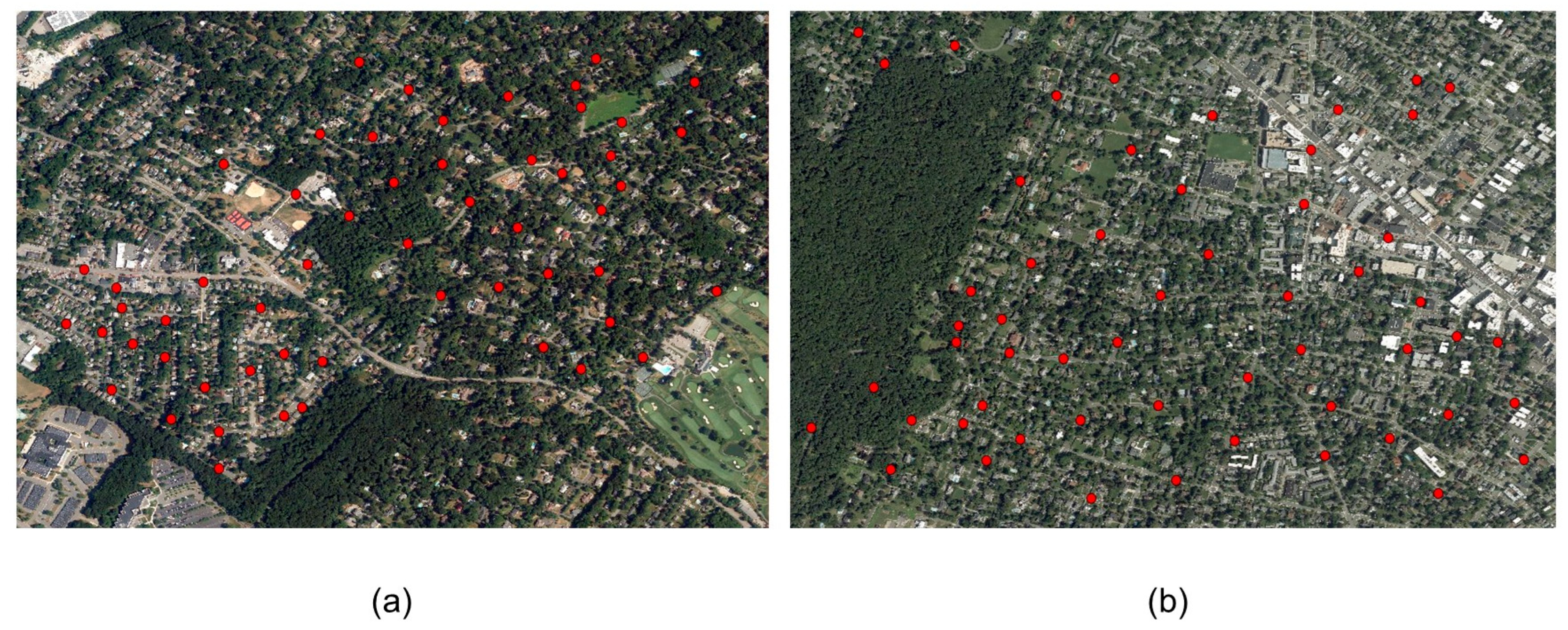
In our efforts to derive environmental properties from aerial and street view images representing different environmental settings, we selected two study sites located in the state of New Jersey in the United States. Both sites are three square kilometers in size. One is located in a town with an average household income similar to the median household income of the state of New Jersey. The study site contains mostly residential neighborhoods. The northeast portion is marked by higher-value homes widely spaced out, with abundant greenness in the environment. The southwest portion has clustered lower-value homes with notably less greenness. Study site 2 has a similar average household income but a greater diversity in its environment. On the west side of this site is a nature reservation, and forest is the main land cover. The east side, in contrast, is a busy downtown district with many developments. Residential neighborhoods lie in between, with moderate housing density and sporadic greenness. Figure 1a shows the aerial imagery of site 1, and Figure 1b that of site 2.

Aerial imageries with a 30 cm spatial resolution were obtained from the USA NAIP multispectral digital orthophoto database for both study sites. Supervised classification was utilized following the previous fine-scale study [27] to identify a set of environmental elements comparable to those identified from street view images. Both pixel-based image classification and object-based image classification were experimented with using ArcGIS Pro 3.0. Training samples were digitized as polygons to capture variant instances of the major environmental elements present in the two study sites, including trees, grass/lawn, roads, rooftops, barren land, water, and artificial surfaces. Rooftops had subclasses with different colors. The Maximum Likelihood Classification (MLC) method was first used following previous studies [27,28]. The Support Vector Machine (SVM) classifier built in ArcGIS Pro 3.0 was also tested. While MLC assumes normal distribution and classifies pixels by maximizing probability, SVM is a non-parametric classifier that seeks an optimal separating hyperplane to maximize the distance between each class in an N-dimensional space, making it more robust to non-normal distributions and complex datasets. A range of settings of spectral and spatial details and minimum segment sizes was also tested. Close visual inspections on the resulting maps were conducted to choose an optimal classified map for each site that required minor manual re-classifications.

After manual re-classifications, the final classified images were used to derive environmental properties within fixed-distance buffers around locations where GSV images were randomly sampled in the two study sites. Buffer sizes of 30 m, 60 m, and 100 m were experimented with. The choice of a 30 m buffer was based on previous fine-scale studies [27,28] on environmental properties’ effect on humans’ psychological states. The choice of 100 m was because common buffer sizes used by a variety of previous studies are often 100 m+ [18,19,20,21,22,25,29,35]. The 60 m buffer is in the middle of the two, double the 30 m buffer size. The percentage of the area in the buffers was calculated for each of the major environmental elements following the previous fine-scale studies [27,28].

A total of 110 locations were randomly sampled from the two study sites (55 in each) and street view panoramas were downloaded from the GSV repository. Figure 1 also shows the GSV locations. Two image segmentation approaches were employed to identify the specific environmental elements corresponding to those classified from aerial images. The first approach utilized a pre-trained DeepLabV3 model [48] using the ResNet-101 backbone [49]. DeepLab is a semantic segmentation model based on deep learning, which uses atrous convolutions to capture multi-scale contextual information without the need to greatly reduce spatial resolution. DeepLabV3 also uses improved Atrous Spatial Pyramid Pooling (ASPP) to consider objects at different scales and segment with much improved accuracy. Equation (1) describes the atrous convolution algorithm [source: 48]. With two-dimensional signals, for each location i on the output y and a filter w, atrous convolution is applied over the input feature map x following Equation (1), where the atrous rate r corresponds to the stride with which the input signal is sampled, equivalent to convolving the input x with up-sampled filters produced by inserting r − 1 zeros between two consecutive filter values along each spatial dimension.

$$y\left[i\right]=\sum _{k}x\left[i+r\ast k\right]w\left[k\right]$$

(1)

The ResNet-101 backbone adopts a 101-layer deep convolutional neural network (CNN) known for its strong feature extraction capabilities by using “skip connections” to overcome the vanishing gradient problem [49]. The Microsoft COCO dataset [50] was used for training the model. It is a large-scale image dataset used for training and benchmarking computer vision models for object detection, segmentation, and captioning tasks. It comprises over 330,000 images containing about 1.5 million object instances across 80 common object categories. The dataset includes detailed annotations for object categories, bounding boxes, pixel-level segmentation masks, and multiple captions per image, making it a widely used dataset for large-scale object detection and segmentation applications.

The second approach utilized the PaddleSeg image segmentation toolkit version 2.9 [51] with the PP-LiteSeg model for semantic segmentation [52]. PaddleSeg is a high-efficiency, open-source toolkit for image segmentation based on Baidu’s PaddlePaddle deep learning framework [51]. It supports a wide range of segmentation capabilities, including semantic segmentation. The toolkit has a modular structure, supporting various mainstream segmentation network architectures, among which PP-LiteSeg is a convolutional neural network incorporating a lightweight encoder–decoder structure in order to optimize both speed and accuracy. It does not rely on a specific pre-trained backbone. The key modules in PP-LiteSeg—the Flexible and Lightweight Decoder (FLD), Spatial–Temporal Deformable Convolution (STDC), Unified Attention Fusion Module (UAFM), and Simple Pyramid Pooling Module (SPPM)—are designed to enhance segmentation performance while reducing computational cost. These modules make the model more efficient compared to the traditional deep CNNs like ResNet. We utilized the Cityscapes [53] and Mapillary Vistas datasets [54] as training data to segment environmental elements. The Cityscapes dataset contains 5000 annotated images with fine annotations and 20,000 more images with coarse annotations from fifty cities around the world. The Mapillary Vistas dataset contains 25,000 manually annotated images from around the world, featuring diverse conditions and geographic locations. Both are known for their use in street scenes, with the former particularly in urban street scenes.

3. Results

3.1. Image Classification with Aerial Images

Pixel-based image classification was found to be limited in its ability to differentiate between ambiguous pixels with similar spectral signatures, such as trees and grass in many areas as well as rooftops and some paved road surfaces in others. This resulted in speckled surfaces that would require extensive amounts of manual reclassification. Object-based classification with the SVM method required extra steps to create effective training samples but resulted in much cleaner classified images that required less manual reclassification. Figure 2 and Figure 3 show the classified images for site 1 and 2, respectively. With 60 randomly located testing samples used for each site, the classification accuracies assessed for site 1 and site 2 are 93.3% (56 out of 60 samples were correctly classified) and 95% (57 out of 60 samples were correctly classified), respectively.

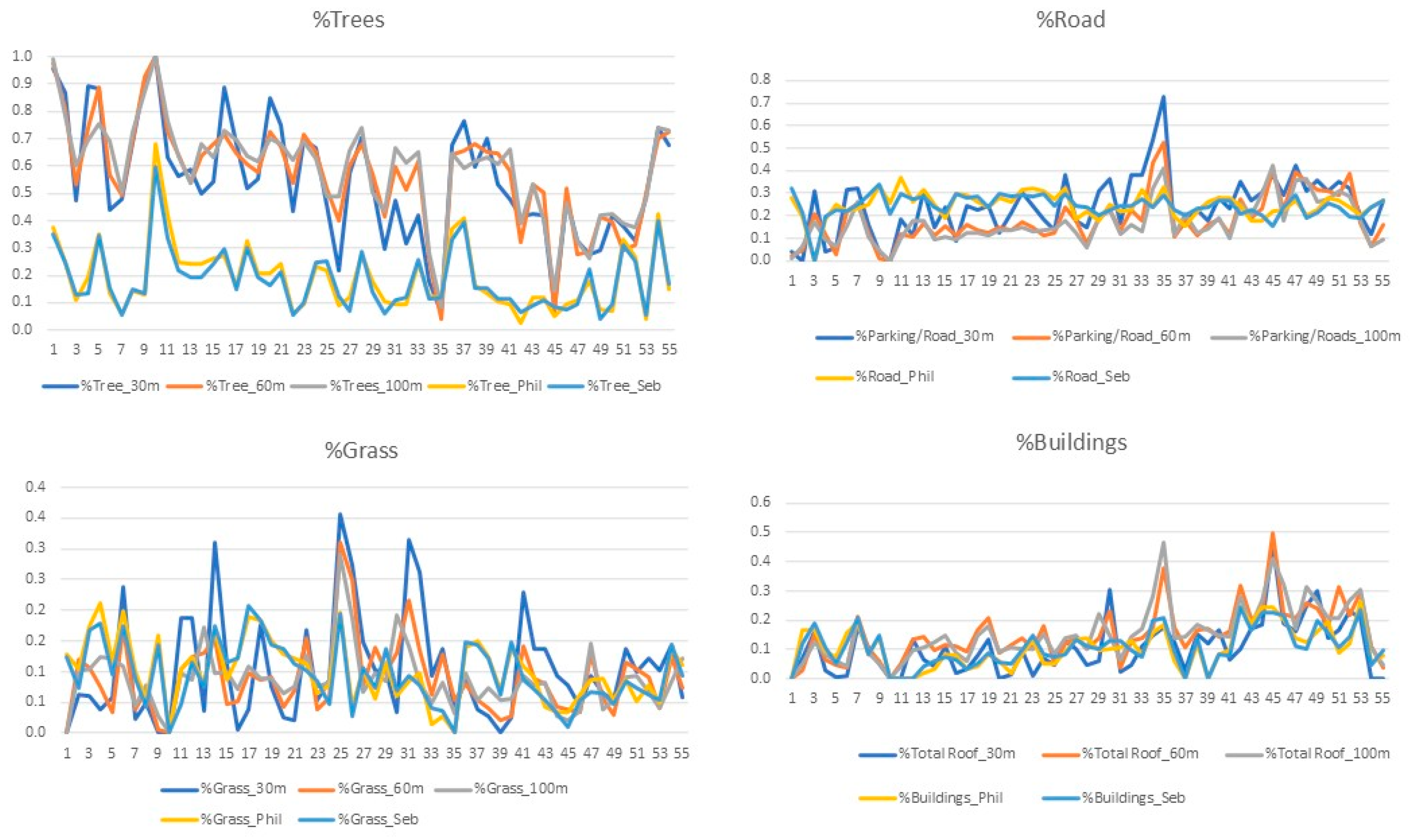
Figure 4 shows the proportions of four major environmental elements calculated within the three buffer sizes in study site 1. The amount of water, barren land, and artificial surface are quite limited in the study site and thus we did not include them in the figures. We grouped different colored rooftops together to account for all buildings. The data is sorted according to the percentage of trees with the 30 m buffer size.

Table 1. Average proportions of environmental elements with different buffer sizes in study site 1.

Buffer Size	%Trees	%Grass	%Roads	%Roof	%Water
30 m	57.24%	15.48%	9.97%	17.22%	0.03%
60 m	58.83%	16.53%	8.66%	15.83%	0.08%
100 m	59.79%	16.12%	8.69%	15.11%	0.13%

lists the average proportions of these environmental elements with different buffer sizes. The table includes water, in order to show its limited amount. It is noted that the average proportions of the natural elements, trees, grass, and water generally increase with the increase in buffer sizes. The proportions of the artificial elements, rooftops, and roads show opposite trends. The overall differences among the three buffer sizes are not significant. Both Table 1 and Figure 4 also show that the proportions of these various environmental elements calculated using the 60 m and 100 m buffer sizes are very similar. For trees, when the tree coverage is between 40% and 80% (based on the 30 m buffer), all three buffer sizes show similar results. When the environment has little tree coverage (<30%), larger buffer sizes, such as 60 m and 100 m, lead to higher proportions of trees in the calculation than the 30 m buffer. When the environment has extensive tree coverage (>80%), the larger buffers lead to lower percentages of trees. It is also observed that less tree coverage tends to lead to higher percentages of rooftops when using a small buffer (30 m) compared to the larger ones (60 m and 100 m). With extensive tree coverage (>80%), the differences among buffer sizes diminish. Roads and grass do not show similar consistent trends.

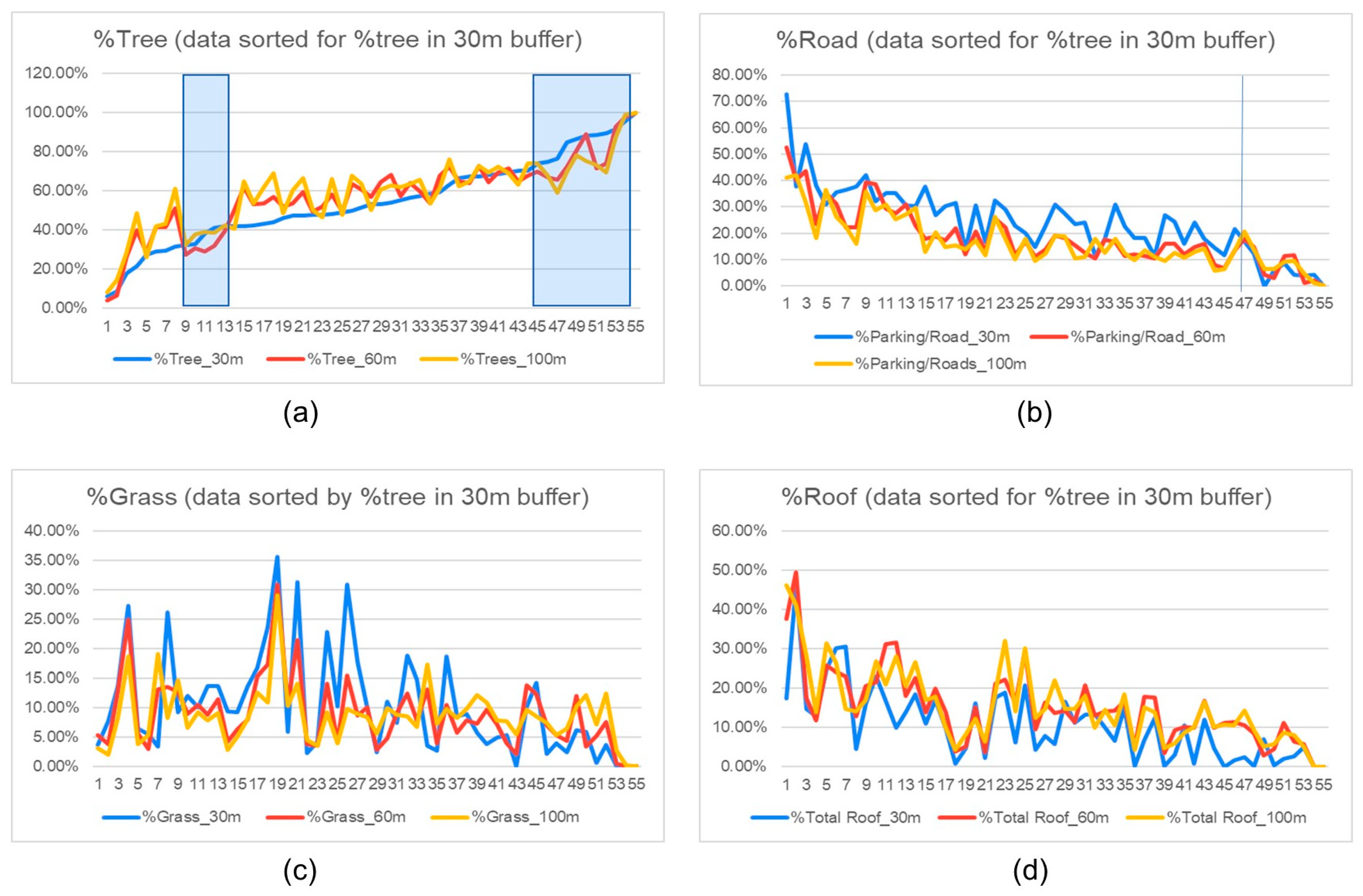
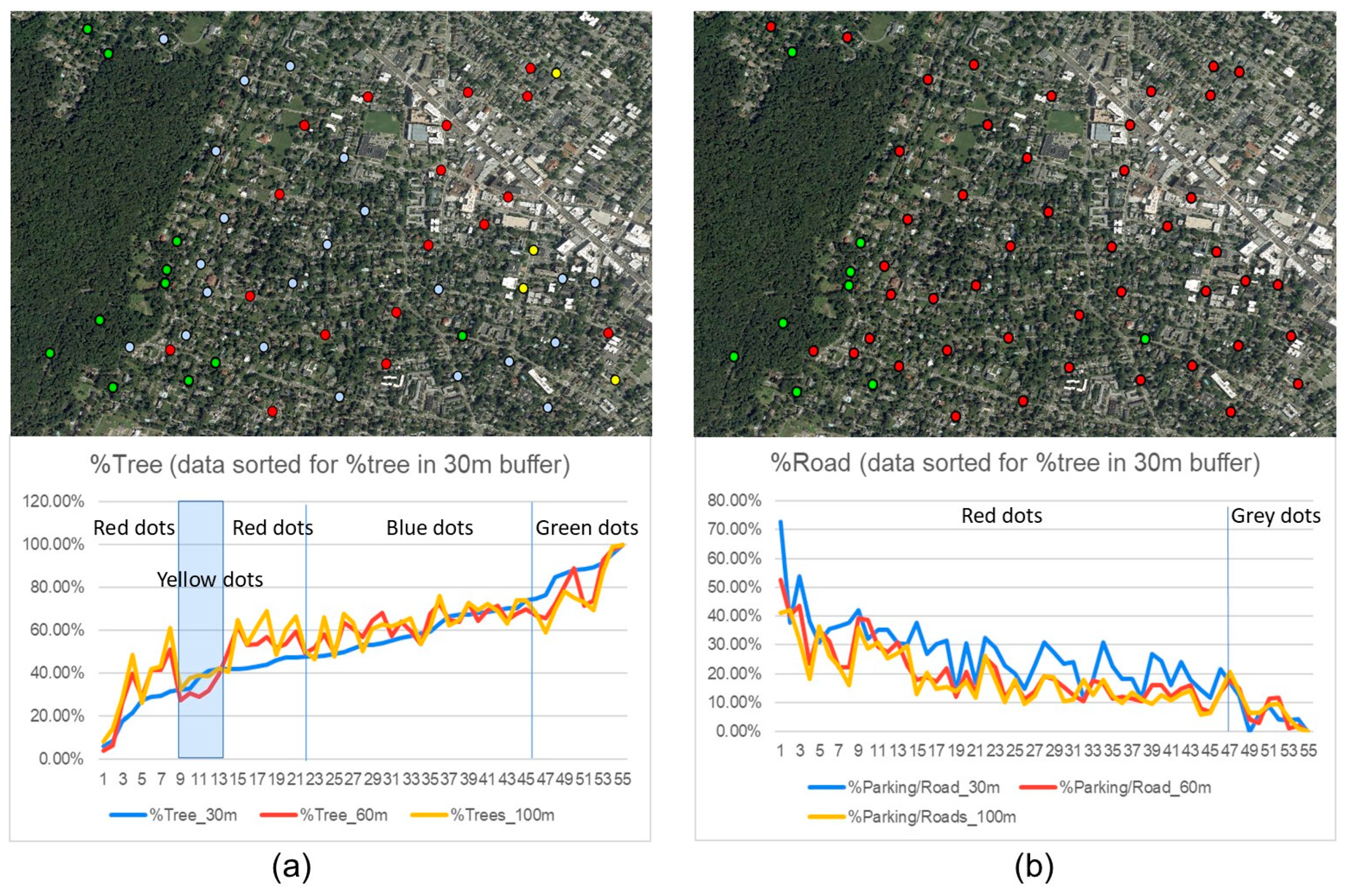
Figure 5 shows the proportions of the same four major environmental elements calculated within the three buffer sizes in study site 2.

Table 2. Average proportions of environmental elements with different buffer sizes in study site 2.

Buffer Size	%Trees	%Grass	%Roads	%Roof	%Water
30 m	54.83%	10.23%	24.12%	10.57%	0.01%
60 m	57.43%	8.88%	18.30%	15.11%	0.11%
100 m	58.68%	8.65%	16.80%	15.40%	0.19%

lists the average proportions of these environmental elements with the different buffer sizes. It shows a slightly different pattern from that of site 1. The proportions of trees and water still increase as the buffer size becomes larger, but grass proportions do not. The proportions of roads still increase with the buffer size, but those of rooftops decrease instead. Figure 5 also shows different patterns from study site 1. When there is extensive tree coverage (>70% with 30 m buffer, shown by the blue shaded area to the right in Figure 5a), the proportion of trees is highest in the smallest buffer size among the three. The three buffer sizes generate similar tree proportions when the tree coverage is between 30% and 40% within the 30 m buffers (the blue shaded area to the left in Figure 5a), while larger buffers generate greater proportions of trees at all other locations. The calculated proportions of roads are always higher when using the smallest buffer size among the three. The proportions of roof areas are always lower using the 30 m buffer. Similarly to site 1, grass does not show a consistent trend, and buffer sizes of both 60 m and 100 m still show similar results for most elements.

3.2. Image Segmentation with Street View Images

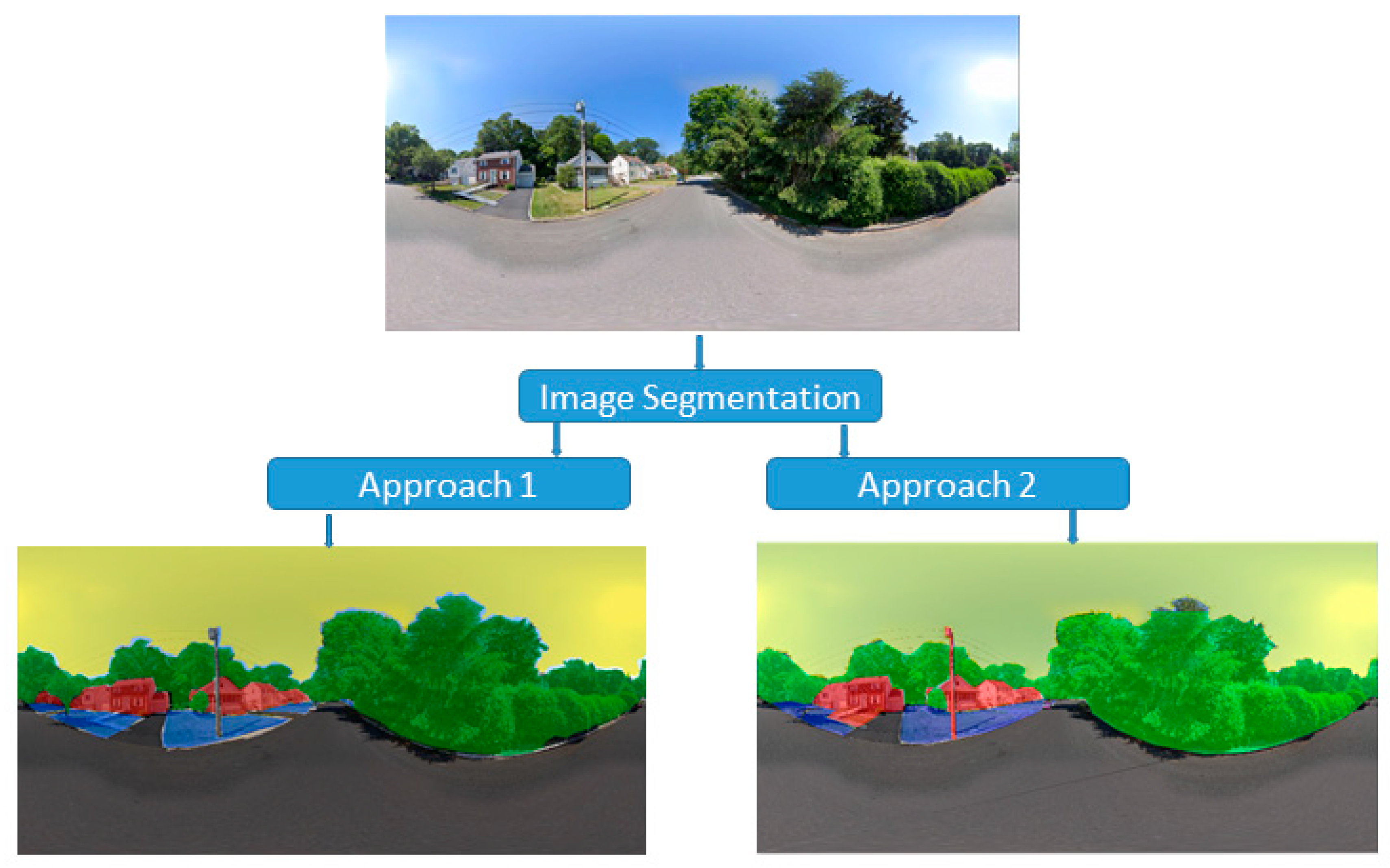
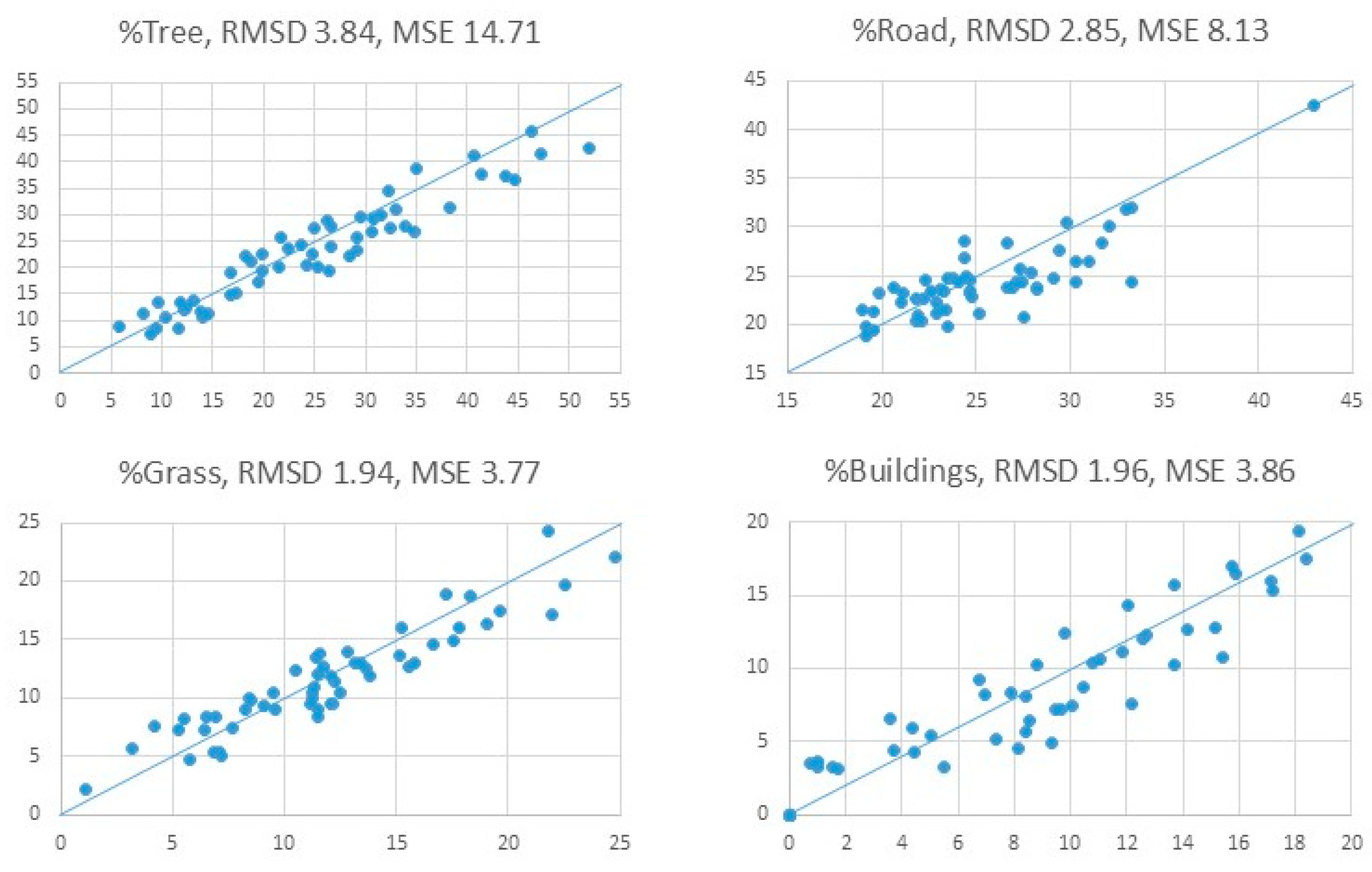
Figure 6 and Figure 7 show the segmented images of two GSVs in our samples using the two image segmentation approaches. The two results bear a good level of similarity. One notable difference is that the edges of treetops are segmented as grass when using the first approach. Figure 8 and Figure 9 show the scatterplots comparing the results of the two image segmentation approaches for study sites 1 and 2, respectively. We focused on the four major environmental elements in the aerial images. It is observable that the two approaches are agree more with regard to the natural elements, like trees and grass, than the artificial elements, like roads and houses. There is a higher degree of agreement for the natural elements in site 2 than in site 1 according to the calculated RMSDs. It is the opposite for artificial elements, for which site 1 shows a higher degree of agreement, especially with regard to the percentage of roads.

3.3. Comparison Between Results from Aerial Image Classification and Street View Image Segmentation

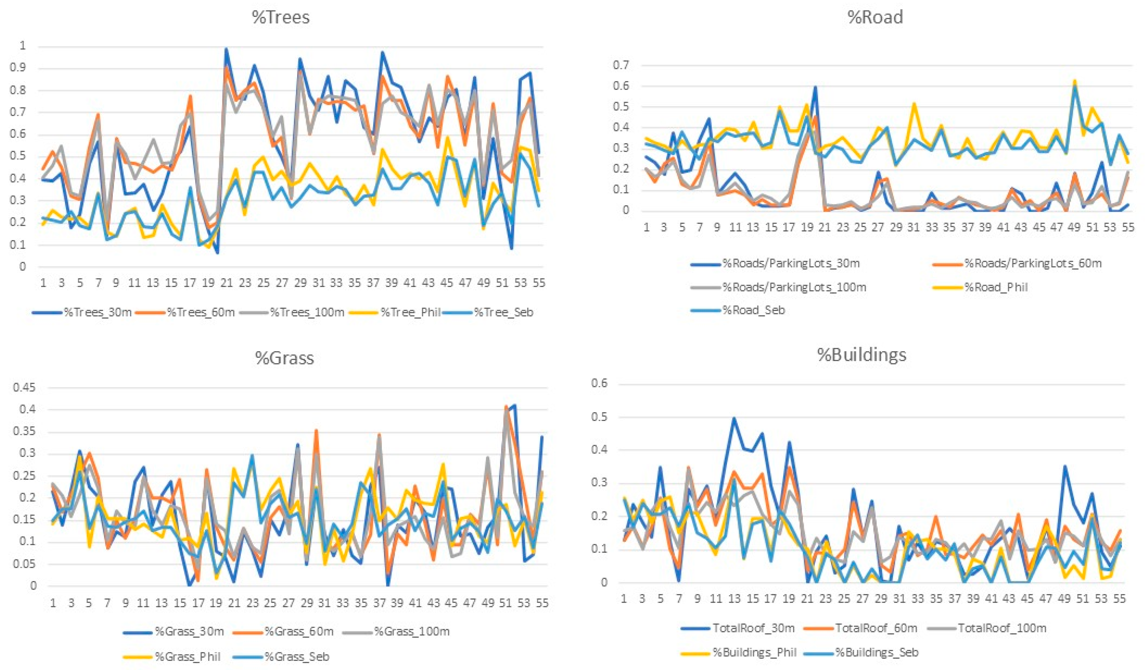
Figure 10 and Figure 11 show the comparisons of the percentages of the different environmental elements calculated from classified aerial images and segmented street view images for sites 1 and 2, respectively. The following is observed for site 1: (1) for trees, percentages calculated from aerial images are always higher than those from the street view images, regardless of the buffer sizes used, (2) for roads it is the opposite, and (3) grass and buildings do not show consistent patterns. The results for site 2 are slightly different. The percentages of trees are still higher when derived from aerial images with all buffer sizes than when derived from street view images. Buffer sizes of 60 m and 100 m, however, show a much closer match with the results from street view images. Likewise, the percentages of roads derived from aerial images with 60 m and 100 m buffers are more consistent with those from street view images than the other buffer sizes. The percentage of grass derived from aerial images versus from street view images do not show much concordance in site 1, but the percentage of buildings are somewhat agreeable.

Table 3. Correlation coefficients between percentages of trees derived from aerial and from GSV images for study site 1.

Methods	Aerial 30 m Buffer	Aerial 60 m Buffer	Aerial 100 m Buffer	GSV Approach 1
Aerial 60 m buffer	0.9170
Aerial 100 m buffer	0.8914	0.9627
GSV approach 1	0.7654	0.7255	0.6806
GSV approach 2	0.7819	0.7498	0.7108	0.9531

,

Table 4. Correlation coefficients between percentages of roads derived from aerial and from GSV images for study site 1.

Methods	Aerial 30 m Buffer	Aerial 60 m Buffer	Aerial 100 m Buffer	GSV Approach 1
Aerial 60 m buffer	0.9180
Aerial 100 m buffer	0.8728	0.9594
GSV approach 1	0.2443	0.2488	0.2527
GSV approach 2	0.2269	0.2797	0.2922	0.8836

,

Table 5. Correlation coefficients between percentages of grass derived from aerial and from GSV images for study site 1.

Methods	Aerial 30 m Buffer	Aerial 60 m Buffer	Aerial 100 m Buffer	GSV Approach 1
Aerial 60 m buffer	0.7965
Aerial 100 m buffer	0.7189	0.9242
GSV approach 1	0.0819	−0.0058	0.0474
GSV approach 2	0.0822	−0.0168	−0.0096	0.9298

and

Table 6. Correlation coefficients between percentages of buildings derived from aerial and from GSV images for study site 1.

Methods	Aerial 30 m Buffer	Aerial 60 m Buffer	Aerial 100 m Buffer	GSV Approach 1
Aerial 60 m buffer	0.8868
Aerial 100 m buffer	0.7997	0.8919
GSV approach 1	0.3933	0.4205	0.4436
GSV approach 2	0.4497	0.4609	0.4916	0.9428

list the Pearson correlation coefficients for study site 1. The percentages of trees show fair correlation between those derived from aerial and from street view images, and the highest correlation is with a 30 m buffer zone. The percentages of grass and roads are not correlated between those derived from aerial and from street view images. The percentages of buildings are somewhat correlated, with slightly higher correlations as buffer sizes increase. Among those percentages derived from aerial images, the 60 m and 100 m are always highly correlated, especially for trees and roads. This is consistent with the pattern observed in Figure 4. Between the two image segmentation approaches, correlation is the most significant for trees and buildings.

Table 7. Correlation coefficients between percentages of trees derived from aerial and from GSV images for study site 2.

Methods	Aerial 30 m Buffer	Aerial 60 m Buffer	Aerial 100 m Buffer	GSV Approach 1
Aerial 60 m buffer	0.9189
Aerial 100 m buffer	0.8656	0.9620
GSV approach 1	0.5641	0.5239	0.5162
GSV approach 2	0.5416	0.4963	0.4949	0.9730

,

Table 8. Correlation coefficients between percentages of roads derived from aerial and from GSV images for study site 2.

Methods	Aerial 30 m Buffer	Aerial 60 m Buffer	Aerial 100 m Buffer	GSV Approach 1
Aerial 60 m buffer	0.8886
Aerial 100 m buffer	0.7933	0.9389
GSV approach 1	0.2765	0.2235	0.1660
GSV approach 2	0.2090	0.1560	0.0907	0.8875

,

Table 9. Correlation coefficients between percentages of grass derived from aerial and from GSV images for study site 2.

Methods	Aerial 30 m Buffer	Aerial 60 m Buffer	Aerial 100 m Buffer	GSV Approach 1
Aerial 60 m buffer	0.8195
Aerial 100 m buffer	0.5218	0.8252
GSV approach 1	0.1642	0.2189	0.3161
GSV approach 2	0.1418	0.2068	0.3071	0.9474

and

Table 10. Correlation coefficients between percentages of buildings derived from aerial and from GSV images for study site 2.

Methods	Aerial 30 m Buffer	Aerial 60 m Buffer	Aerial 100 m Buffer	GSV Approach 1
Aerial 60 m buffer	0.8298
Aerial 100 m buffer	0.7586	0.9065
GSV approach 1	0.5574	0.5840	0.6318
GSV approach 2	0.5927	0.6241	0.6772	0.9511

list the correlation coefficients for study site 2. The percentages of trees derived from aerial images and from street view images are not correlated as much as those for site 1. The correlations for buildings, on the other hand, are higher than site 1. The most significant correlation for trees is with a 30 m buffer, while for buildings it is 100 m. Like site 1, roads and grasses are not correlated. Among the three buffer sizes, the 60 m and 100 m buffers are still more correlated than the 30 m buffer size for all environmental elements. The two image segmentation approaches correlate well for trees, buildings, and grass for this site, and they, in general, correlate better with each other than they do for site 1.

4. Discussion

4.1. Buffer Sizes for Deriving Environmental Properties from Aerial Images

Table 1 and Figure 4 showed that calculated proportions of the natural elements (trees and grass) generally increase as buffer sizes become larger for study site 1. The calculated proportions of the artificial elements, rooftops, and roads show an opposite trend. This can be explained by the fact that the sample points are in the middle of roads, where GSV images are typically collected. Small buffer sizes thus incorporate extensive areas of roads and the surrounding buildings. Larger buffers can include more natural elements farther away from roads. Site 2 is slightly different (Table 2 and Figure 5), with grass and roads excluded from the above trends. This is because site 2 has both a much more developed downtown and residential neighborhoods (Figure 1). Larger buffers still cover a significant amount of roof and road surfaces. It has also been noted that the overall differences in calculated percentages among the three buffer sizes are not significant for most environmental elements in site 1. However, there is a significant difference among buffer sizes for site 2. This indicates how the choices of buffer sizes should take into consideration the type of environmental settings, especially with regard to densely developed suburban environments. In both study sites, the proportions of all environmental elements calculated using the 60 m and 100 m buffer sizes are very similar. As suggested in our previous study [26], a 30 m buffer captures the immediate environment within one’s visibility range to match humans’ visual perceptions. The calculated environmental properties are no longer sensitive to buffer sizes when buffers grow larger than the immediate visible environment.

4.2. Effects of Different Environmental Settings on Buffer Choices

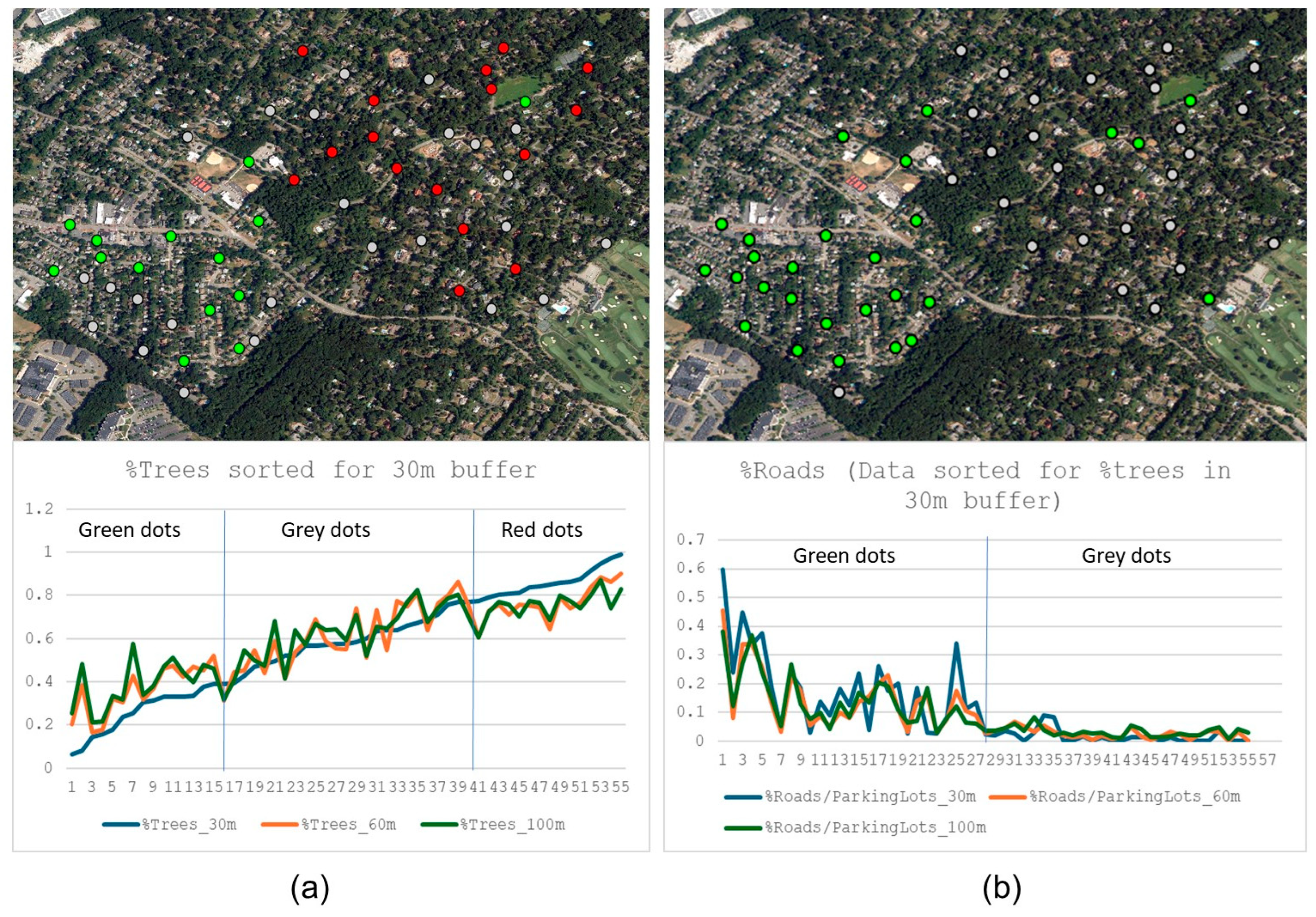
To examine the effects of different environmental settings in more detail, we created Figure 12 which shows two maps differentiating sample locations in slightly different environmental settings. In Figure 12a, the green dots on the image are locations with less than 30% tree coverage when using the 30 m buffers in the chart below. The map shows that they are in areas with the least greenness in this study site. These locations show greater tree percentages with the larger buffer sizes (60 m and 100 m) than the small buffer (30 m), as shown in Figure 4a (as shown to the left of the first blue line). This could be because when the immediate environment has extensive pavements (roads and buildings), expanding the buffer allows for more greenness in the less than immediate vicinity to be accounted for. The red dots on the image are locations with more than 80% tree coverage when using the 30 m buffers in the chart below. The map shows that they are located in areas with the highest level of greenness in this study site. At these locations, the percentages of tree coverage are higher when using the 30 m buffers than the 60 m and 100 m (Figure 4a, right of the second blue line). This is because when there are a lot of trees in the neighborhood, the tree canopies cover much of the rooftops on the sides of the streets in the immediate environment. Expanding the buffers allows more buildings to be accounted for. This is confirmed by Figure 4d, in which the 80% tree coverage is also the threshold for rooftops. The gray dots are in between, where all three buffer sizes show comparable tree percentages.

Figure 12b differentiates two types of locations for the percentage of roads calculated. The green dots on the image above show where road areas calculated within a 30 m buffer are slightly higher than other buffer sizes, as shown in the chart beneath the image. The gray dots on the image above show where all three buffers have similar percentages of roads in the chart below. This indicates that when greenness is limited in the environment, a 30 m buffer captures more immediate road area, especially since our sample locations are in the middle of the roads where GSV images are collected. When a considerable amount of greenness exists in the neighborhood, the road area drops to a very low percentage in the buffers. So, the buffer sizes we chose no longer make a notable difference.

Figure 13 shows the maps with different color-coded location types in study site 2. In Figure 13a, the red dots show locations with the least greenness, where the calculated percentages of trees are higher with 60 m and 100 m buffers compared to 30 m buffers. There are a few exceptions, such as the yellow dots, where the three buffers show similar results. The green dots show locations with the most greenness in this study site, where the calculated percentages of trees are higher with a 30 m buffer than the larger buffers. The blue dots are in between, where the three buffer sizes yield similar results. This pattern is the same as that observed in study site 1. The yellow dots are exceptions because they are not only surrounded by extensive developments (roads and buildings) in the immediate environment captured by the 30 m buffer, but they are also close to either large buildings or parking lots in the extended vicinity captured by the 60 m or 100 m buffers. Thus, expanding the buffer size did not result in increased tree cover.

Figure 13b, like the case with study site 1, shows that when there is limited greenness in the environment, a 30 m buffer captures more immediate road area, thus resulting in higher percentages of road surfaces than the larger buffers. By looking into the different types of locations of our sample points, we observe that it is not the overall study site that differentiates our results, but the specific environmental settings of different types of neighborhoods at a smaller scale. The environment of each study site is heterogeneous, containing neighborhoods ranging from very limited trees to abundant tree coverage. The choice of buffer sizes should consider the specific environmental settings within a study area. One consistent observation is that 60 m and 100 m buffers often lead to similar results for a variety of environmental elements and across a spectrum of environmental settings.

4.3. Effects of Different Environmental Settings on GSV Image Segmentation

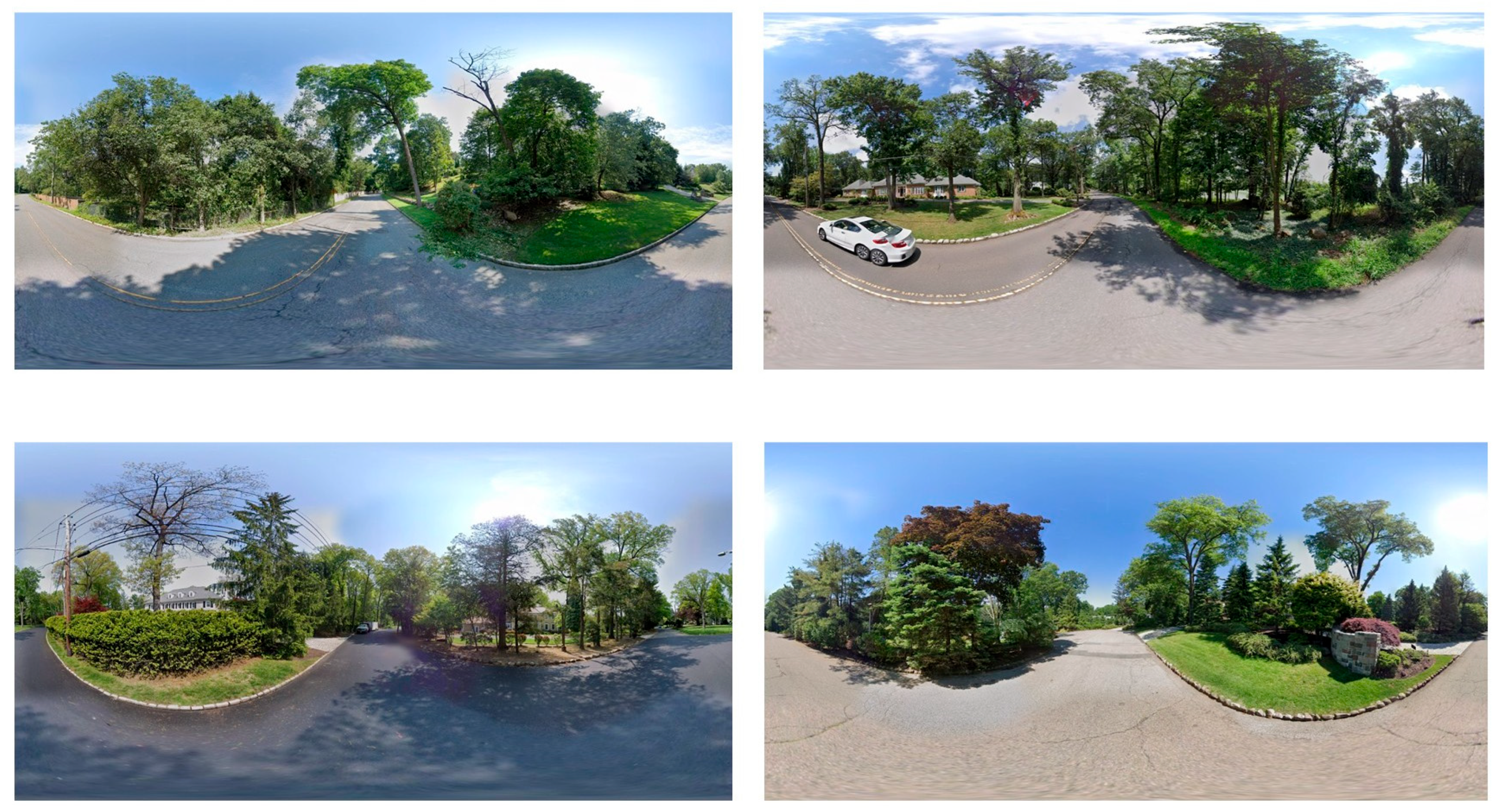
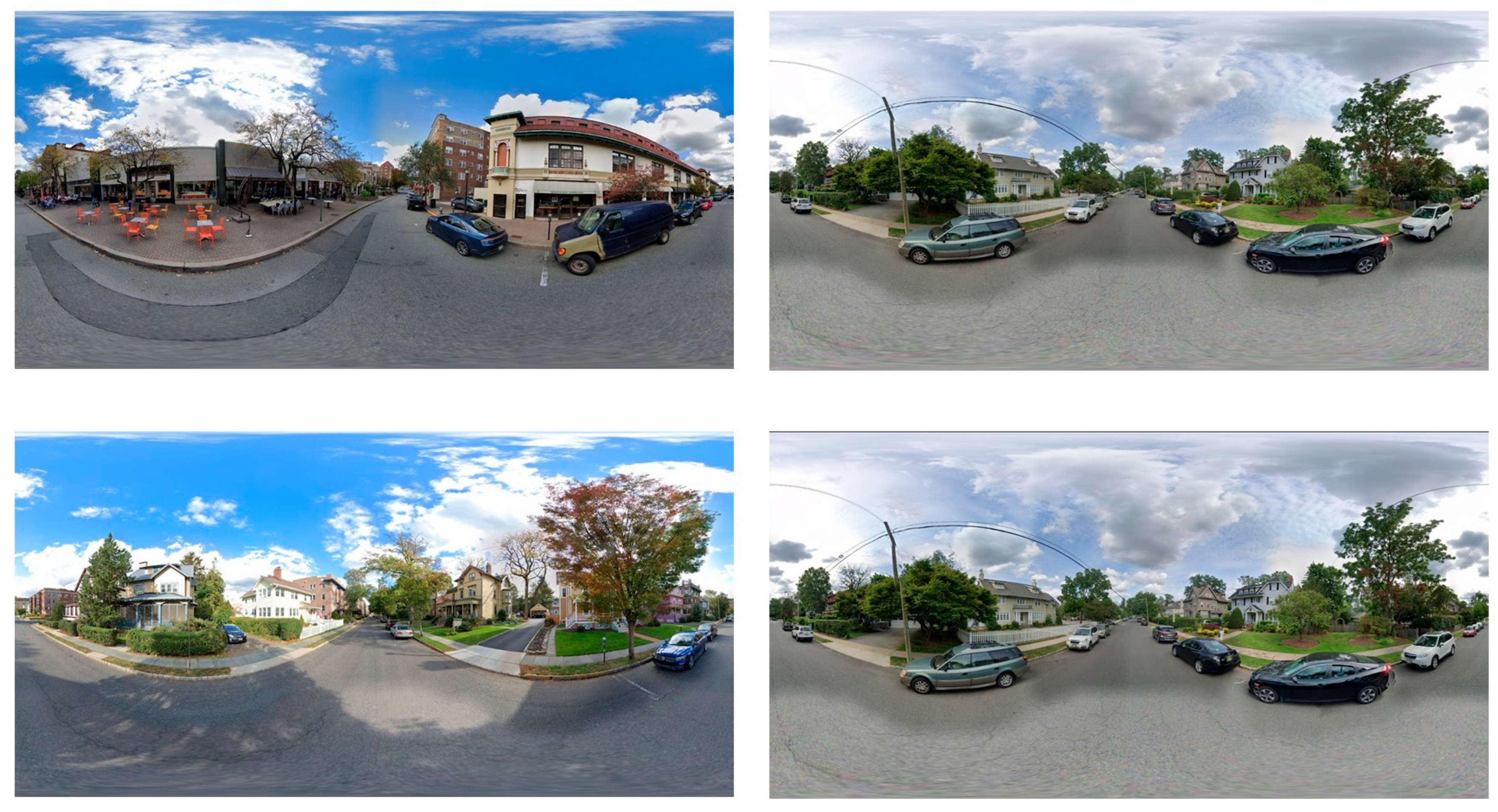
The scatterplots in Figure 8 and Figure 9 show that the two image segmentation approaches employed are highly agreeable in terms of the natural elements (trees and grass) and less so in terms of the artificial elements (roads and buildings). There is also a higher degree of agreement between the two approaches for the natural elements in site 2 than in site 1 while the opposite is true for artificial elements, for which site 1 shows a higher degree of agreement, especially with regard to the percentage of roads. Figure 14 and Figure 15 show some representative GSV images from the two study sites. In study site 1 (Figure 14), most residential neighborhoods have a good number of trees, while in site 2 (Figure 15), one third of the area is a densely developed downtown community (top two GSV images) and the residential neighborhoods do not have as many trees as those in study site 1. Although there is a nature reservation on the west side of the site, being limited by the GSV collection methods, no GSV images are available in those areas. The different environmental settings of these two study sites could have been one of the causes of differentiating results using our two image segmentation approaches. One other cause could be the algorithms and training data used. Due to the scale of this current study, we were not able to generate a customized training dataset and testing dataset for our specific study sites. Thus, we were not able to measure the accuracy of the two approaches. It is our belief that using customized training data should considerably increase accuracy for image segmentation. In future efforts, GSV images representing the environmental characteristics of the study area could be manually annotated and used as training data to improve segmentation accuracy as well as selecting the best segmentation method.

4.4. Correspondences of Environmental Elements Derived from Aerial and Street View Images

When we compared the results from the segmented GSV images to those from the classified aerial images (Table 3, Table 4, Table 5, Table 6, Table 7, Table 8, Table 9 and Table 10), the agreements of derived environmental elements decrease in the order of trees, buildings, roads, and then grass. A direct reason is that tree canopies block lawns and some road surfaces in the aerial view. Trees correspond between the two better in a greener environment (study site 1) while buildings correspond better in a more developed environment (study site 2). In other words, the most prominent environmental elements in a particular environment show the best correspondences between aerial and street view images. Another finding is that the absolute percentages of trees calculated from aerial images are always higher than those calculated from street view images (Figure 10 and Figure 11). For roads, the opposite is observed. The reason is that tree canopies often cover road surfaces in aerial images, while for GSV images, road surfaces are often exaggerated as in all panoramic images (Figure 14 and Figure 15).

When we examined the correspondences between aerial and GSV images with regard to the buffer sizes experimented with, the best agreements for trees were with a 30 m buffer. For buildings it was 60 m or 100 m. This can be explained by the fact that trees and their leaves in the immediate environment of an observer can easily block humans’ visibility of objects beyond 30 m, and this the same for street view photos, impacting what they can capture. The buildings in our study site, as with most suburban neighborhoods in New Jersey, are low-rise. Visibility could thus easily reach 60 m or 100 m. We speculate that in big cities with high-rise buildings, small buffer sizes would have better correspondences between aerial and street view images.

In street view images, sky usually accounts for a high percentage of the segmented images. Aerial images do not contain the sky element. In an attempt to examine the impact of this discrepancy on the environmental properties that were derived from the images, we removed the sky element from the GSV images and recalculated the percentages.

Table 11. Correlation coefficients between percentages of trees derived from aerial and from GSV images adjusted for sky for study site 1.

Methods	Aerial 30 m Buffer	Aerial 60 m Buffer	Aerial 100 m Buffer	GSV Approach 1
Aerial 60 m buffer	0.9170
Aerial 100 m buffer	0.8914	0.9627
GSV approach 1	0.7396	0.7163	0.6890
GSV approach 2	0.7467	0.7306	0.7134	0.9359

,

Table 12. Correlation coefficients between percentages of roads derived from aerial and from GSV images adjusted for sky for study site 1.

Methods	Aerial 30 m Buffer	Aerial 60 m Buffer	Aerial 100 m Buffer	GSV Approach 1
Aerial 60 m buffer	0.9180
Aerial 100 m buffer	0.8728	0.9594
GSV approach 1	0.3298	0.3181	0.3233
GSV approach 2	0.3525	0.3754	0.3832	0.9010

,

Table 13. Correlation coefficients between percentages of grass derived from aerial and from GSV images adjusted for sky or study site 1.

Methods	Aerial 30 m Buffer	Aerial 60 m Buffer	Aerial 100 m Buffer	GSV Approach 1
Aerial 60 m buffer	0.7964
Aerial 100 m buffer	0.7189	0.9242
GSV approach 1	0.1974	0.1139	0.1545
GSV approach 2	0.2258	0.1154	0.1039	0.9043

,

Table 14. Correlation coefficients between percentages of buildings derived from aerial and from GSV images adjusted for sky for study site 1.

Methods	Aerial 30 m Buffer	Aerial 60 m Buffer	Aerial 100 m Buffer	GSV Approach 1
Aerial 60 m buffer	0.8868
Aerial 100 m buffer	0.7997	0.8919
GSV approach 1	0.4581	0.4684	0.4766
GSV approach 2	0.5084	0.5074	0.5259	0.9526

,

Table 15. Correlation coefficients between percentages of trees derived from aerial and from GSV images adjusted for sky for study site 2.

Methods	Aerial 30 m Buffer	Aerial 60 m Buffer	Aerial 100 m Buffer	GSV Approach 1
Aerial 60 m buffer	0.9189
Aerial 100 m buffer	0.8656	0.9620
GSV approach 1	0.5816	0.5592	0.5436
GSV approach 2	0.5518	0.5287	0.5260	0.9635

,

Table 16. Correlation coefficients between percentages of roads derived from aerial and from GSV images adjusted for sky for study site 2.

Methods	Aerial 30 m Buffer	Aerial 60 m Buffer	Aerial 100 m Buffer	GSV Approach 1
Aerial 60 m buffer	0.8886
Aerial 100 m buffer	0.7933	0.9389
GSV approach 1	0.5062	0.4739	0.4391
GSV approach 2	0.4634	0.4209	0.3914	0.9277

,

Table 17. Correlation coefficients between percentages of grass derived from aerial and from GSV images adjusted for sky or study site 2.

Methods	Aerial 30 m Buffer	Aerial 60 m Buffer	Aerial 100 m Buffer	GSV Approach 1
Aerial 60 m buffer	0.8195
Aerial 100 m buffer	0.5218	0.8252
GSV approach 1	0.1898	0.2514	0.3295
GSV approach 2	0.1546	0.2258	0.3125	0.9497

and

Table 18. Correlation coefficients between percentages of buildings derived from aerial and from GSV images adjusted for sky for study site 2.

Methods	Aerial 30 m Buffer	Aerial 60 m Buffer	Aerial 100 m Buffer	GSV Approach 1
Aerial 60 m buffer	0.8298
Aerial 100 m buffer	0.7586	0.9065
GSV approach 1	0.5596	0.5547	0.5891
GSV approach 2	0.5817	0.5862	0.6266	0.9578

list the new correlation coefficients between the aerial and street view images for the two study sites. In study site 1, the correlation greatly increased for grass, somewhat increased for roads and buildings, but decreased for trees (Table 3, Table 4, Table 5 and Table 6). In study site 2, the correlation also increased for roads and grass significantly, and less so for building (Table 7, Table 8, Table 9 and Table 10). A slight decrease was observed for trees like study site 1. Regardless of the slight decrease in the correlation coefficients, trees were still the most correlated between the aerial and street view images. The removal of sky from street view images caused the percentages of other elements to be larger, which could have caused slightly higher correlations. However, grass and roads were still not correlated significantly between the aerial and street view images. One reason is that these elements are more visible at eye level than in an aerial view, as they are easily covered by tree canopy. In Figure 14 and Figure 15, we notice how the road surfaces are exaggerated considerably in GSV images. This could be another reason why the road element shows poor correlations between the aerial and street views.

5. Conclusions

As studies continue to investigate the relationships between environmental settings and humans’ mental wellbeing using aerial and/or street view images, it is necessary to examine how the environmental properties derived from these two types of images correlate with each other for their use as compensating factors or combine them as composite indices. Our hypotheses included the following: (1) The amount of greenness and individual environmental elements derived from the two types of images may be different. (2) Some environmental elements might have greater concordances between the two than others. (3) The agreements might be greater in some environmental settings. (4) There may exist a buffer size with which the two are more agreeable and thus both could be used together.

Firstly, our experiments showed that among the four major environmental elements examined, the coverage of trees that is calculated from aerial images with varying buffer sizes is always higher than those derived from street view images. That of roads is the opposite. This confirms our first hypothesis. Secondly, among the different environmental elements, trees are in the most concordance between the aerial and street views. Buildings are somewhat agreeable, while grass and roads are not. This confirms our second hypothesis. Thirdly, in residential neighborhoods with abundant greenness (study site 1), the coverage of trees corresponds better than in largely developed environments with limited greenness (study site 2). Buildings show the opposite pattern. This confirms our third hypothesis. And lastly, for the three buffer sizes experimented with for aerial images, trees are in greater concordance with street view images using the 30 m buffer. Low-rise buildings and grass agree better with the larger buffer sizes (60 m and 100 m), especially in relatively open environments. Roads agree better with larger buffers in green environments, but with smaller buffers in less green environments. This indicates that no single buffer size is optimal for all environmental elements and environmental settings, which disconfirms our fourth hypothesis. The choice of which buffer size to use when combining environmental properties derived from aerial and street view images together should consider both the environmental elements involved and the heterogeneity of environmental settings.

The current study is limited in scale as our two study sites are both located in the state of New Jersey in the United States. Although the two sites have different types of neighborhoods, their differences do not capture a wide range of environmental settings. Future studies could include more environmental types. Furthermore, our image segmentation approaches were based on well-established algorithms and existing training datasets. Limited by the scale of our study, we did not use a customized training dataset. Future studies at larger scales could collect a set of street view images to be annotated manually for such purposes. Our study also found the large areas of sky and roads in GSV images affect their concordances with aerial images. In future studies, preprocessing strategies could be considered before segmenting the GSV images, such as truncating the images to leave out the top and bottom quarters (or another portion, worth experimenting to find out) to better match a person’s visual field.

References

1. Parsons, R. The potential influences of environmental perception on human health. J. Environ. Psychol. 1991, 11, 1–23. [Google Scholar] [CrossRef]
2. Fernández Núñez, M.B.; Campos Suzman, L.; Maneja, R.; Bach, A.; Marquet, O.; Anguelovski, I.; Knobel, P. Gender and sex differences in urban greenness’ mental health benefits: A systematic review. Health Place 2022, 76, 102864. [Google Scholar] [CrossRef] [PubMed]
3. White, M.P.; Alcock, I.; Wheeler, B.W.; Depledge, M.H. Would you be happier living in a greener urban area? A fixed effects analysis of panel data. Psychol. Sci. 2013, 24, 920–928. [Google Scholar] [CrossRef] [PubMed]
4. Ulrich, R.S. Aesthetic and affective response to natural environment. In Behavior and the Natural Environment: Vol. 6. Human Behavior and Environment; Altman, I., Wohlwill, J.F., Eds.; Plenum Press: New York, NY, USA, 1983; pp. 85–125. [Google Scholar]
5. Ulrich, R.S.; Simons, R.F.; Losito, B.D.; Fiorito, E.; Miles, M.A.; Zelson, M. Stress recovery during exposure to natural and urban environments. J. Environ. Psychol. 1991, 11, 201–230. [Google Scholar] [CrossRef]
6. Kobayashi, H.; Song, C.; Ikei, H.; Park, B.-J.; Lee, J.; Kagawa, T. Population-based study on the effect of a forest environment on salivary cortisol concentration. Int. J. Environ. Res. Public Health 2017, 14, E931. [Google Scholar] [CrossRef] [PubMed]
7. Hunter, M.R.; Gillespie, B.W.; Chen, S.Y. Urban nature experiences reduce stress in the context of daily life based on salivary biomarkers. Front. Psychol. 2019, 10, 722. [Google Scholar] [CrossRef]
8. van den Berg, A.E.; Maas, J.; Verheij, R.A.; Groenewegen, P.P. Green space as a buffer between stressful life events and health. Soc. Sci. Med. 2010, 70, 1203–1210. [Google Scholar] [CrossRef]
9. Collins, R.; Spake, R.; Brown, K.A.; Ogutu, B.; Smith, D.; Eigenbrod, F. A systematic map of research exploring the effect of greenspace on mental health. Landsc. Urban Plan. 2020, 201, 103823. [Google Scholar] [CrossRef]
10. Berman, M.G.; Ethan, K.; Krpan, K.M.; Askren, M.K.; Burson, A.; Deldin, P.J.; Jonides, J. Interacting with nature improves cognition and affect for individuals with depression. J. Affect. Disord. 2012, 140, 300–305. [Google Scholar] [CrossRef] [PubMed]
11. McCaffrey, R. The effect of healing gardens and art therapy on older adults with mild to moderate depression. Holist. Nurs. Pract. 2007, 21, 79–84. [Google Scholar] [CrossRef]
12. Beyer, K.M.; Kaltenbach, A.; Szabo, A.; Bogar, S.; Nieto, F.; Malecki, K. Exposure to neighborhood green space and mental health: Evidence from the Survey of the Health of Wisconsin. Int. J. Environ. Res. Public Health 2014, 11, 3453–3472. [Google Scholar] [CrossRef]
13. Maas, J.; Verheij, R.A.; De Vries, S.; Spreeuwenberg, P.; Schellevis, F.G.; Groenewegen, P.P. Morbidity is related to a green living environment. J. Epidemiol. Community Health 2009, 63, 967–973. [Google Scholar] [CrossRef]
14. Syamili, M.S.; Takala, T.; Korrensalo, A.; Tuittila, E.-S. Happiness in urban green spaces: A systematic literature review. Urban For. Urban Green. 2023, 86, 128042. [Google Scholar] [CrossRef]
15. Pierpaolo, M.; Dorota, J.; Kendrovski, V.; Braubach, M.; de Vries, S.; Lammel, A.; Andreucci, M. Green and Blue Openspaces and Mental Health: New Evidence and Perspectives for Action. World Health Organization (WHO) Report 2021. Available online: https://www.who.int/europe/publications/i/item/9789289055666 (accessed on 18 June 2025).
16. UNECE (United Nations Economic Commission for Europe). Sustainable Urban and Peri-Urban Forestry: An Integrative and Inclusive Nature-Based Solution for Green Recovery and Sustainable, Healthy and Resilient Cities. Policy Brief; United Nations: New York, NY, USA, 2021; Available online: https://unece.org/forestry-timber/documents/2023/02/informal-documents/policy-brief-sustainable-urban-and-peri-urban (accessed on 20 June 2025).
17. Wang, R.; Helbich, M.; Yao, Y.; Zhang, J.; Liu, P.; Yuan, Y.; Liu, Y. Urban greenery and mental wellbeing in adults: Cross-sectional mediation analyses on multiple pathways across different greenery measures. Environ. Res. 2019, 176, 108535. [Google Scholar] [CrossRef]
18. Helbich, M.; Poppe, R.; Oberski, D.; van Emmichoven, M.Z.; Schram, R. Can’t see the wood for the trees? An assessment of street view- and satellite-derived greenness measures in relation to mental health. Landsc. Urban Plan. 2021, 214, 104181. [Google Scholar] [CrossRef]
19. Helbich, M.; Yao, Y.; Liu, Y.; Zhang, J.; Liu, P.; Wang, R. Using deep learning to examine street view green and blue spaces and their associations with geriatric depression in Beijing, China. Environ. Int. 2019, 126, 107–117. [Google Scholar] [CrossRef]
20. Wang, R.; Feng, Z.; Pearce, J.; Liu, Y.; Dong, G. Are greenspace quantity and quality associated with mental health through different mechanisms in Guangzhou, China: A comparison study using street view data. Environ. Pollut. 2021, 290, 117976. [Google Scholar] [CrossRef]
21. Houlden, V.; de Albuquerque, J.P.; Weich, S.; Jarvis, S. A spatial analysis of proximate greenspace and mental wellbeing in London. Appl. Geogr. 2019, 109, 102036. [Google Scholar] [CrossRef]
22. Villeneuve, P.J.; Ysseldyk, R.L.; Root, A.; Ambrose, S.; DiMuzio, J.; Kumar, N.; Shehata, M.; Xi, M.; Seed, E.; Li, X.; et al. Comparing the Normalized Difference Vegetation Index with the Google Street View Measure of Vegetation to Assess Associations between Greenness, Walkability, Recreational Physical Activity, and Health in Ottawa, Canada. Int. J. Environ. Res. Public Health 2018, 15, 1719. [Google Scholar] [CrossRef] [PubMed]
23. Larkin, A.; Hystad, P. Evaluating street view exposure measures of visible green space for health research. J. Expo. Sci. Environ. Epidemiol. 2019, 29, 447–456. [Google Scholar] [CrossRef] [PubMed]
24. Bai, Y.; Wang, R.; Yang, L.; Ling, Y.; Cao, M. The Impacts of Visible Green Spaces on the Mental well-being of University Students. Appl. Spat. Anal. 2024, 17, 1105–1127. [Google Scholar] [CrossRef]
25. Liu, Y.; Wang, R.; Lu, Y.; Li, Z.; Chen, H.; Cao, M.; Zhang, Y.; Song, Y. Natural outdoor environment, neighbourhood social cohesion and mental health: Using multilevel structural equation modelling, streetscape and remote-sensing metrics. Urban For. Urban Green. 2020, 48, 126576. [Google Scholar] [CrossRef]
26. Stubbings, P.; Peskett, J.; Rowe, F.; Arribas-Bel, D. A Hierarchical Urban Forest Index Using Street-Level Imagery and Deep Learning. Remote Sens. 2019, 11, 1395. [Google Scholar] [CrossRef]
27. Qi, F.; Parra, A.O.; Block-Lerner, J.; McManus, J. Psychological Impacts of Urban Environmental Settings: A Micro-Scale Study on a University Campus. Urban Sci. 2024, 8, 73. [Google Scholar] [CrossRef]
28. Wang, F.; Qi, F. Urban Environment and Momentary Psychological States: A Micro-Scale Study on a University Campus with Network Analysis. Urban Sci. 2025, 9, 221. [Google Scholar] [CrossRef]
29. Rieves, E.S.; Reid, C.E.; Carlson, K.; Li, X. Do environmental attitudes and personal characteristics influence how people perceive their exposure to green spaces? Landsc. Urban Plan. 2024, 248, 105080. [Google Scholar] [CrossRef]
30. Hua, J.; Cai, M.; Shi, Y.; Ren, C.; Xie, J.; Chung, L.C.H.; Lu, Y.; Chen, L.; Yu, Z.; Webster, C. Investigating pedestrian-level greenery in urban forms in a high-density city for urban planning. Sustain. Cities Soc. 2022, 80, 103755. [Google Scholar] [CrossRef]
31. Zhang, L.; Wang, L.; Wu, J.; Li, P.; Dong, J.; Wang, T. Decoding urban green spaces: Deep learning and google street view measure greening structures. Urban For. Urban Green. 2023, 87, 128028. [Google Scholar] [CrossRef]
32. Xia, Y.; Yabuki, N.; Fukuda, T. Development of a system for assessing the quality of urban street-level greenery using street view images and deep learning. Urban For. Urban Green. 2021, 59, 126995. [Google Scholar] [CrossRef]
33. Zhang, X.; Lin, E.S.; Tan, P.Y.; Qi, J.; Waykool, R. Assessment of visual landscape quality of urban green spaces using image-based metrics derived from perceived sensory dimensions. Environ. Impact Assess. Rev. 2023, 102, 107200. [Google Scholar] [CrossRef]
34. Chen, C.; Li, H.; Luo, W.; Xie, J.; Yao, J.; Wu, L.; Xia, Y. Predicting the effect of street environment on residents’ mood states in large urban areas using machine learning and street view images. Sci. Total Environ. 2022, 816, 151605. [Google Scholar] [CrossRef]
35. Liu, Y.; Xiao, T.; Liu, Y.; Yao, Y.; Wang, R. Natural outdoor environments and subjective well-being in Guangzhou, China: Comparing different measures of access. Urban For. Urban Green. 2021, 59, 127027. [Google Scholar] [CrossRef]
36. Jiang, B.; Deal, B.; Pan, H.Z.; Larsen, L.; Hsieh, C.H.; Chang, C.Y.; Sullivan, W.C. Remotely-sensed imagery vs. eye-level photography: Evaluating associations among measurements of tree cover density. Landsc. Urban Plan. 2017, 157, 270–281. [Google Scholar] [CrossRef]
37. Ye, Y.; Richards, D.; Lu, Y.; Song, X.; Zhuang, Y.; Zeng, W.; Zhong, T. Measuring daily accessed street greenery: A human-scale approach for informing better urban planning practices. Landsc. Urban Plan. 2019, 191, 103434. [Google Scholar] [CrossRef]
38. Wagner, M.; Květoňová, V.; Jirmus, R.; Lehnert, M. Towards greener cities: Evaluating urban green space accessibility using the 3-30-300 rule exampled on the city of Olomouc (Czech Republic). Morav. Geogr. Rep. 2025, 33, 129–142. [Google Scholar] [CrossRef]
39. Lee, S.; Kim, Y.; Koo, B.W. Urban trees and perceived neighborhood safety: Neighborhood upkeep matters. Environ. Behav. 2024, 56, 276–321. [Google Scholar] [CrossRef]
40. Peng, H.; Zhu, T.; Yang, T.; Zeng, M.; Tan, S.; Yan, L. Depression or recovery? A study of the influencing elements of urban street environments to alleviate mental stress. Front. Archit. Res. 2025, 14, 846–862. [Google Scholar] [CrossRef]
41. Huang, Y.; Zhong, C.; He, T.; Jiang, Y. Dynamics of street environmental features and emotional responses in urban areas: Implications for public health and sustainable development. Front. Public Health 2025, 13, 1589183. [Google Scholar] [CrossRef]
42. Lu, X.; Li, Q.; Ji, X.; Sun, D.; Meng, Y.; Yu, Y.; Lyu, M. Impact of streetscape built environment characteristics on human perceptions using street view imagery and deep learning: A case study of Changbai Island, Shenyang. Buildings 2025, 15, 1524. [Google Scholar] [CrossRef]
43. Ho, L.C.; Wei, Y.T.; Li, D.; Chiang, Y.C. Revealing emotional responses to urban environmental elements through street view data and deep learning. Environ. Plan. B Urban Anal. City Sci. 2025. [Google Scholar] [CrossRef]
44. Ludwig, C.; Hecht, R.; Lautenbach, S.; Schorcht, M.; Zipf, A. Mapping Public Urban Green Spaces Based on OpenStreetMap and Sentinel-2 Imagery Using Belief Functions. ISPRS Int. J. Geo-Inf. 2021, 10, 251. [Google Scholar] [CrossRef]
45. Kaplan, R.; Kaplan, S. The Experience of Nature: A Psychological Perspective; Cambridge University Press: Cambridge, UK, 1989. [Google Scholar]
46. Kaplan, S. The restorative benefits of nature: Toward an integrative framework. J. Environ. Psychol. 1996, 15, 169–182. [Google Scholar] [CrossRef]
47. Velasquez-Camacho, L.; Etxegarai, M.; de-Miguel, S. Implementing Deep Learning algorithms for urban tree detection and geolocation with high-resolution aerial, satellite, and ground-level images. Comput. Environ. Urban Syst. 2023, 105, 102025. [Google Scholar] [CrossRef]
48. Chen, L.C.; Papandreou, G.; Kokkinos, I.; Murphy, K.; Yuille, A.L. DeepLab: Semantic image segmentation with deep convolutional nets, atrous convolution, and fully connected CRFs. IEEE Trans. Pattern Anal. Mach. Intell. 2017, 40, 834–848. [Google Scholar] [CrossRef]
49. He, K.; Zhang, X.; Ren, S.; Sun, J. Deep residual learning for image recognition. In Proceedings of the IEEE Conference on Computer Vision and Pattern Recognition (CVPR), Las Vegas, NV, USA, 27–30 June 2016; pp. 770–778. [Google Scholar]
50. Lin, T.Y.; Maire, M.; Belongie, S.; Hays, J.; Perona, P.; Ramanan, D.; Dollár, P.; Zitnick, C.L. Microsoft COCO: Common objects in context. In Proceedings of the European Conference on Computer Vision, Zurich, Switzerland, 6–12 September 2014; pp. 740–755. [Google Scholar]
51. Liu, Y.; Chu, L.; Chen, G.; Wu, Z.; Chen, Z.; Lai, B.; Hao, Y. PADDLESEG: A high-efficient development toolkit for Image segmentation. arXiv 2021, arXiv:2101.06175. Available online: https://arxiv.org/abs/2101.06175 (accessed on 20 June 2025).
52. Peng, J.; Liu, Y.; Tang, S.; Hao, Y.; Chu, L.; Chen, G.; Wu, Z.; Chen, Z.; Yu, Z.; Du, Y. PP-LiteSeg: A superior real-time semantic segmentation model. arXiv 2022, arXiv:2204.02681. Available online: https://arxiv.org/abs/2204.02681 (accessed on 20 June 2025).
53. Cordts, M.; Omran, M.; Ramos, S.; Rehfeld, T.; Enzweiler, M.; Benenson, R.; Franke, U.; Roth, S.; Schiele, B. The cityscapes dataset for Semantic Urban Scene understanding. In Proceedings of the 2016 IEEE Conference on Computer Vision and Pattern Recognition (CVPR), Las Vegas, NV, USA, 27–30 June 2016; pp. 3213–3223. Available online: https://openaccess.thecvf.com/content_cvpr_2016/html/Cordts_The_Cityscapes_Dataset_CVPR_2016_paper.html (accessed on 20 June 2025).
54. Neuhold, G.; Ollmann, T.; Rota Bulo, S.; Kontschieder, P. The mapillary vistas dataset for semantic understanding of street scenes. In Proceedings of the IEEE International Conference on Computer Vision, Venice, Italy, 22–29 October 2017; pp. 4990–4999. Available online: https://openaccess.thecvf.com/content_iccv_2017/html/Neuhold_The_Mapillary_Vistas_ICCV_2017_paper.html (accessed on 20 June 2025).
Figure 1. Aerial images for the study sites and the sample locations. (a) study site 1; (b) study site 2.
Urbansci 09 00486 g001
Figure 2. Classified image for study site 1. (a) pixel-based classification; (b) object-based classification.
Urbansci 09 00486 g002
Figure 3. Classified image for study site 2. (a) pixel-based classification; (b) object-based classification.
Urbansci 09 00486 g003
Figure 4. Proportions of four major environmental elements within the three buffer sizes in study site 1. (a) trees; (b) roads; (c) grass; and (d) roof.
Urbansci 09 00486 g004
Figure 5. Proportions of four major environmental elements within the three buffer sizes in study site 2. (a) trees; (b) roads; (c) grass; and (d) roof.
Urbansci 09 00486 g005
Figure 6. Image segmentation results of one GSV image with the two approaches.
Urbansci 09 00486 g006
Figure 7. Image segmentation results of a second GSV image with the two approaches.
Urbansci 09 00486 g007
Figure 8. Scatterplots comparing the results of the two image segmentation approaches for study sites 1.
Urbansci 09 00486 g008
Figure 9. Scatterplots comparing the results of the two image segmentation approaches for study sites 2.
Urbansci 09 00486 g009
Figure 10. Comparisons of percentages of environmental elements calculated from classified aerial images and segmented street view images for site 1.
Urbansci 09 00486 g010
Figure 11. Comparisons of percentages of environmental elements calculated from classified aerial images and segmented street view images for site 2.
Urbansci 09 00486 g011
Figure 12. Differentiating sample locations in different environmental settings in study site 1 with regard to proportions of (a) trees and (b) roads.
Urbansci 09 00486 g012
Figure 13. Differentiating sample locations in different environmental settings in study site 2 with regard to proportions of (a) trees and (b) roads.
Urbansci 09 00486 g013
Figure 14. Representative GSV’s from study site 1.
Urbansci 09 00486 g014
Figure 15. Representative GSV’s from study site 2.
Urbansci 09 00486 g015