Environmental Monitoring in Bus Transportation Using a Developed Measurement System

Abstract

Air pollution and travel comfort in public transport is a significant problem as it can cause health problems for passengers. There are no sufficiently developed and researched monitoring systems for measuring the quality of the environment in public transport, which makes it difficult to assess the extent of the problem and implement effective solutions. This study presents the results of measurements made with a developed system for assessing air pollution and environmental quality in urban transport. Two time periods were defined based on air pollution and traffic levels, and informational features were selected for bus stops and buses. Noise was found not to be an informative feature, but vehicle acceleration should be considered in environmental quality monitoring. A quadratic discriminant classifier combined with principal components was shown to accurately classify high and low pollution time periods. Further research is planned to investigate the relationship between air pollution and travel discomfort and to develop effective strategies to improve air quality in urban public transport.

1. Introduction

Air pollutants are a complex mixture of gases and particles that are released into the air via human activities such as transport, industrial processes, and energy production. Exposure to polluted air is associated with a wide range of adverse health effects, including respiratory and cardiovascular disease, cancer, and premature death. The World Health Organization (https://www.who.int, accessed on 8 May 2023) estimates that outdoor air pollution causes approximately 4.2 million premature deaths worldwide each year.

Buses, trains, and other vehicles that are used for public transportation release pollutants like fine particulate matter (PM), nitrogen oxides (NO_x), and volatile organic compounds (VOCs), which are major sources of air pollution in metropolitan areas [1]. People who spend a lot of time in public transportation environments, such as passengers and employees, are exposed to high quantities of these pollutants, which could have detrimental effects on their health [2].

Air quality monitoring is important and relevant in the context of public transport for the following reasons [3,4,5]:

• Provides crucial insights into the sources and levels of air pollution in public transport environments, offering essential information to inform policies and interventions aimed at reducing exposure and improving the overall air quality. By monitoring air pollution in these settings, the research identifies effective strategies to combat the issue, such as the implementation of cleaner fuels and the adoption of advanced technologies. These findings play a vital role in shaping sustainable solutions and promoting healthier urban environments for commuters and the general public alike;
• Monitoring can help raise awareness among the public and policymakers about the health risks associated with air pollution in public transport and the need for action to address this problem.

The problem is the lack of accurate and reliable air quality data in public transport, so it is necessary to develop and test a mobile measurement system that can provide such data [6]. The acquisition, processing, and analysis of measurement data on pollution levels in urban transport can help to improve the understanding of the sources of air pollution in public transport and can inform the development of policies and interventions to address this problem [7]. There is a complex relationship between air quality, passenger comfort, and acceleration in public transport [8]. Accelerations and decelerations can significantly affect passenger comfort, especially for those who stand or are susceptible to motion sickness. Sharp or sudden movements can cause discomfort, sickness, and even injury. On the other hand, smoother accelerations and decelerations can improve passenger comfort and reduce the likelihood of injury. Air quality is also an essential factor for passenger comfort, as poor air quality can lead to discomfort, respiratory problems, and other health problems [9,10].

Employing smooth and gradual acceleration, along with effective ventilation and air filtration systems, can help maintain high air quality, thereby fostering a comfortable and healthy environment for passengers. However, it is important to acknowledge that the scope and limitations of such research are contingent on specific geographical areas or types of public transport, as well as the technical constraints of measurement systems.

The aim of the present work is to design, develop, and evaluate a mobile measurement system to provide sufficiently accurate and reliable data on environment quality in public transport.

2. Related Work

In recent years, metal oxide gas sensors have established themselves as a popular choice for air quality assessment in urban transport [11,12,13]. One of the trends in their application is the use of miniature and low-power sensors that can be easily integrated into small devices for personal air quality monitoring in vehicles. This allows people to monitor their exposure to air pollutants while commuting to work or engaging in outdoor activities.

Quantified by Veetil [14], among the sources of urban air pollution, 49% of the average air pollution is produced by transport, 28% is produced by fuel burned in factories and power plants, 13% by the evaporation of volatile substances, 3% from municipal solid waste disposal, and 7% from various other sources.

The issue of urban air pollution, as emphasized by Kam et al. [15], is that the toxic emissions from vehicle tailpipes which produce a variety of compounds, such as hydrocarbons (HC), nitrogen oxides (NO_x), carbon monoxide (CO), carbon dioxide (CO₂), particulate matter (PM), and sulfur oxides (SO_x), are designated as the origins of this pollution. In addition to contributing to the acceleration of global warming, these emissions have major detrimental effects on both human health and the environment, including air pollution, smog, acid rain, liver damage, cancer, and heart disease. Addressing the adverse effects of these emissions on both human health and the environment is of utmost importance. Implementing sustainable practices, transitioning to cleaner energy sources, and adopting stringent emission reduction policies are vital steps towards mitigating the impacts of global warming and improving public health and environmental well-being [1,2,5,7,16].

Dahl et al. [17] and Kwak et al. [18] found that non-exhaust particulate emissions result from the re-dispersion of road dust, wear and tear of vehicle parts (such as brakes and tires), and abrasion on the road surface, mainly contributing to the coarse range (from PM2.5 to PM10).

Travel-related factors are directly influenced by the driving mode of road vehicles. Detailed studies [19] state that the travel-related factors depend on the operating modes of the vehicle engine, the speed of the moving vehicle, as well as its accelerations and decelerations (driving mode). Accordingly, the number of trips, distance traveled, and driving mode on a given road are the main travel-related factors affecting emissions. However, Zacharof et al. [20] state that aggressive driving can increase the amount of fuel consumption, which in turn increases air emissions. This means that low speeds, busy driving conditions, sudden acceleration, deceleration, etc., lead to higher emissions.

De Winkel et al. [21] describe the relationship between the properties of vehicle movements, such as acceleration and sudden stops and starts, and the discomfort experienced by the occupants of automated vehicles. The results show that discomfort increases with acceleration amplitude and that higher cuts are considered more comfortable. The study also evaluates normative models of vibration and shock and presents new statistical models that describe ride comfort as a function of acceleration, shock, and direction.

Sun et al. [22] define that comfort in public transport buses mainly depend on noise, temperature, vibration, and acceleration. Among these four factors, vibration and acceleration are the two most significant.

From the analysis of the available literature sources, it can be seen that they are aimed at the analysis of measurements of air quality in the vehicle, and the influence of acceleration and noise. Options for measurement systems and analysis of their operational efficiency are not considered. In addition, the quality of air is not a sufficient criterion for evaluating the travel comfort of passengers in public transport. It is necessary to propose a measurement system that is suitable for a complex study of travel comfort related to the quality characteristics of the environment, including noise and acceleration [23] of the vehicle.

3. Material and Methods

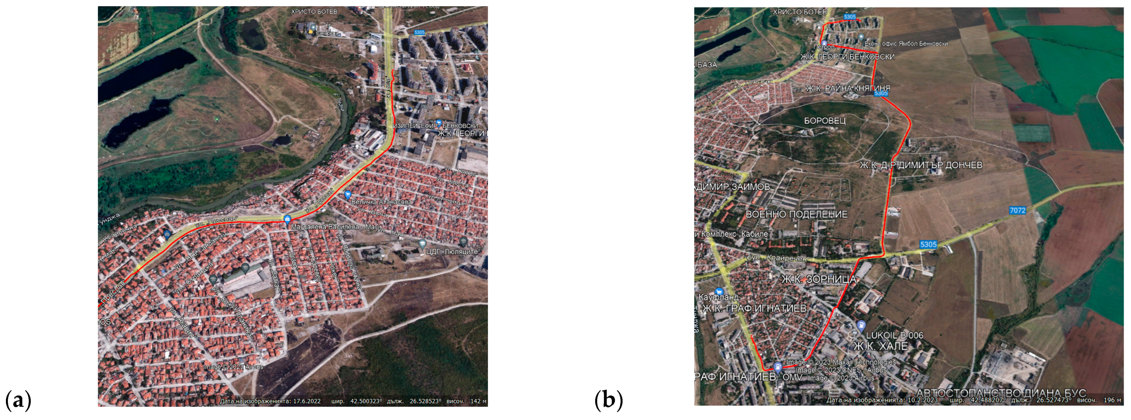
The measurements were made along two lines of the city bus transport in the city of Yambol, Bulgaria. They were carried out along part of the routes of lines #5 and #25. These bus lines have been chosen as representative samples for the entire city bus transport system. By selecting routes that cover diverse areas, such as city centers, outskirts, and different types of neighborhoods, the collected data can provide a comprehensive understanding of pollution patterns across the city.

The public transport buses are renovated, model Graf und Stift (MAN Truck&Bus SE, Munich, Germany), and delivered from Vienna for the transport operator serving the lines in the city. The buses are equipped with security systems, passenger comfort, and an electronic information system. The vehicles are environmentally friendly, according to the Euro 5 standard, as they are powered via a six-cylinder internal combustion engine. Its volume is 12.8 L, with liquefied petroleum gas (LPG) as the main fuel.

Figure 1 shows images of the two surveyed routes. They are represented by a solid red line in the pictures. The first route N° 5 has the start point at 42.487788° N, 26.511111° E and the end point at 42.500713° N, 26.525521° E. All GPS coordinates are in the WGS84 format. The second route N° 25 has the start point at 42.502266° N, 26.525518° E and the end point at 42.473440° N, 26.522112° E.

According to the data from a GPS device, the length of the routes, the speed of the vehicle, and the time spent at the bus stops were determined. The total length of both routes is 6 km. The total travel time is 120 min. The average speed of the buses is 35 km/h, and the maximum speed is 45 km/h. The stay time at the stops is a total of 60 min.

The measurements were taken in heavy and light traffic of people and cars in an urban environment.

The data from the automatic measuring stations installed at six measuring points in the city of Yambol were used. Figure 2 shows a general view of an online portal accessible through the website of the Municipality of Yambol. The portal offers an interactive geographical map with the measurement points. The data are presented for PM2.5, PM10, temperature, relative humidity, and atmospheric pressure. Average values for the levels of the measured characteristics and data on their permissible levels are presented. The portal offers a history of measurements in both graphical and tabular form. The history of measurements can be organized for periods desired by the user.

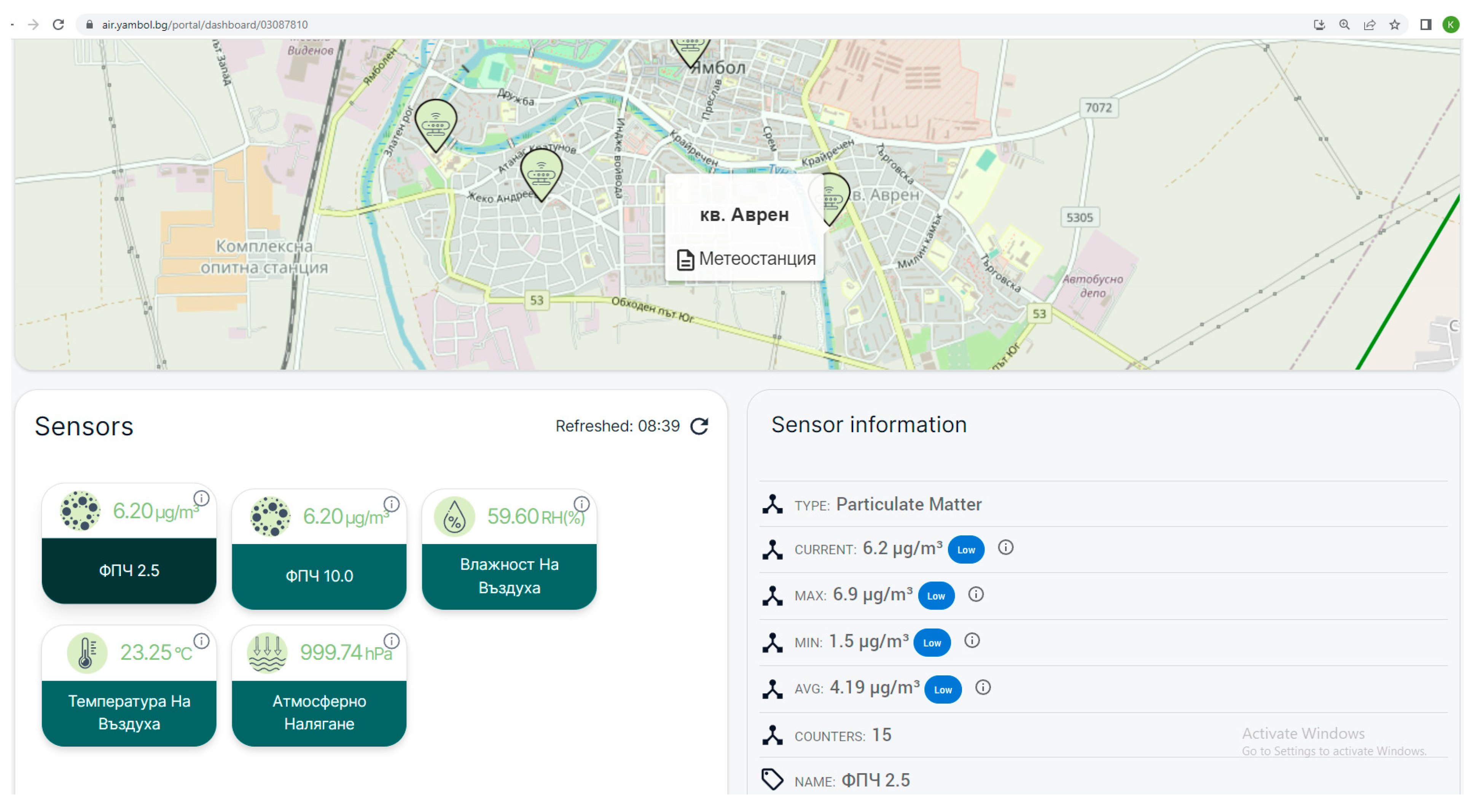
The data from the automatic station are compared with those from the measurement system proposed in this work. The differences in the readings between the two measuring devices do not exceed 10%.

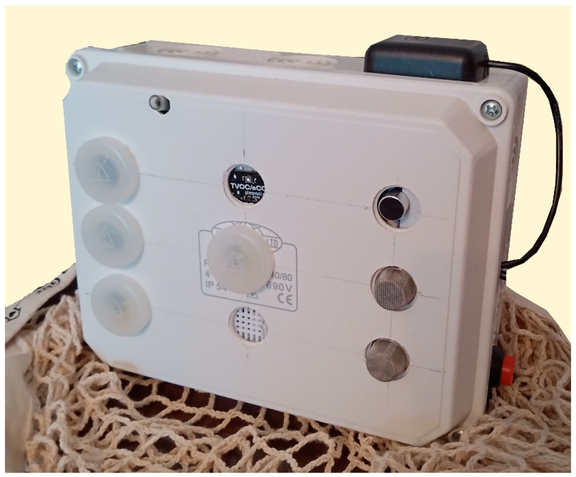
3.1. Sensor Devices

Sensor for temperature and relative air humidity. A DHT22 digital sensor (Aosong (Guangzhou) Electronics Co., Ltd., Guangzhou, China) was selected. The sensor has an operating voltage of 3.3–5 V DC. It measures relative air humidity 0–99% RH, with an accuracy of ±2% (at 25°) and a resolution of down to 0.1%. The temperature is measured in the range of −40–80 °C, with an accuracy of ±0.5 °C and a resolution of 0.1 °C. The refresh rate is 1 Hz (reports are every 1 s). The sensor uses “One Wire” protocol. The “DHT.h” library is used for its work.

Sensor for TVOC, eCO₂, H₂ and ethanol. A digital sensor SGP30 (Pimoroni Ltd., Sheffield, UK) was selected. It is presented in position b. The sensor uses a I²C digital communication interface, with address 0 × 58. It uses the libraries <Wire.h> and “Adafruit_SGP30.h”. The device can measure the concentration of four gases simultaneously. TVOC and eCO₂ are preset by the manufacturer. H₂ and ethanol are obtained as a decimal value from the ADC of the sensor. The sensor has automatic humidity and temperature compensation. In order to be able to use the data from the last two gases, a conversion is required, which is specified in the technical specification (Datasheet) of the sensor:

$$C=C_{ref}.e^{\left(\frac{S_{ref}-S_{out}}{512}\right)}, \mathrm{ppm}$$

(1)

where C, ppm is the concentration of the corresponding gas; S_ref is the ADC reference value at 0.5 ppm of the respective gas; S_out is the data from the ADC when measuring (dimensionless quantity). For ethanol, C_ref = 0.4 ppm, and for H₂, C_ref = 0.5 ppm. Reference values of S_ref have been determined at 0.5 ppm of the respective gas. For H₂, S_ref = 14,055, and for ethanol, S_ref = 19,831. The reference data is dimensionless because it represents an output value from the sensor’s ADC.

Accelerometer. An ADXL345 accelerometer (Analog Devices, Inc., Wilmington, NC, USA) was selected. The three-axis digital accelerometer and gyroscope is an ADXL345 integrated circuit-based module. The module is small, thin, and has low power consumption, allowing for measurement with a sufficiently high resolution (13-bit) up to ±16 g. The digital output data is formatted as 16-bit (complementary) and is accessible via SPI or I²C interfaces. The ADXL345 is suitable for portable device applications. Its high milligram resolution (3.9 mg/LSB) allows for measurement of tilt changes of less than 1.0°. The module works with voltage: 4–6 V DC. It offers two options for serial synchronous communication, SPI and I²C. The DC current consumption is 23 µA in measurement mode. Library <Adafruit_ADXL345_U.h> is used to work with the module.

Noise sensor. A Sound Sensor module (Waveshare Electronics, Shenzhen, China) was used. The module is built from an electret microphone with a range of 50–20,000 Hz. The microphone signal is amplified via an LM386 operational amplifier. The module has a gain factor of 200. The microphone has a sensitivity of 52 dB. The supply voltage of the sensor module is 3.3–5.3 V DC. The determination of the loudness in dB was performed using a program code proposed in [24]. The noise level in dB is calculated after reading the analog output of the sensor in a window of 50 ms.

Sensor for NO_x, SO_x and O₃. An MQ-135 sensor (Waveshare Electronics, Shenzhen, China) was used. Through this sensor, the total amount of sulfur and nitrogen oxides, as well as ozone, was determined. The data from the analog output of the sensor is fed to the analog input of the single-board microcomputer. The conversion of the data obtained from the ADC into the voltage values is in the range 0–5 V. From the measured voltage obtained at the analog output of the sensor, the resistance of the sensor can be calculated according to the following dependencies:

$$U=ADC\frac{5}{1023}, \mathrm{V}$$

(2)

$$R_s=\left(\frac{5}{U}-1\right)R_L, \mathrm{k}\mathsf{\Omega }$$

(3)

where ADC is the value of the 0–1023 analog-to-digital converter. R_s is the resistance of the sensor; U is the voltage from the analog output of the sensor; and R_L is the load resistance of the sensor.

According to the technical documentation of the sensor, the load resistance of the sensor is R_L = 20.1 kΩ. The resistance of the sensor in clean air is R₀ = 10 kΩ.

A humidity and temperature correction factor has been determined for the MQ-135 sensor. Temperature and relative humidity were measured with a DHT22 sensor. According to the technical documentation of the sensor, the correction equation has the following form:

$$c_f=-0.03T-0.003\left(H-33\right)+0.003T^2+0.000025T\left(H-33\right)$$

(4)

where cf is a correction factor; T, °C is ambient temperature; and H, %RH is relative air humidity.

To determine the concentration of the relevant gas, a model is used, which is more often used in the sensors of the MQ-xxx series. According to the technical documentation of the sensors, these models have the following general appearance:

$${\mathrm{NO}}_{\mathrm{x}},C_{N{O}_x}=116.6{\left(\frac{R_s}{R_0}\right)}^{-2.79},\mathrm{ppm}$$

(5)

$${\mathrm{SO}}_{\mathrm{x}},C_{S{O}_x}=331.51{\left(\frac{R_s}{R_0}\right)}^{-0.97}, \mathrm{ppm}$$

(6)

$${\mathrm{O}}_3,C_{O_3}=9.48{\left(\frac{R_s}{R_0}\right)}^{-2.34}, \mathrm{ppm}$$

(7)

where Cx, ppm is the concentration of the corresponding measured gas, and variables a and b are the model coefficients. The corrected values of (R_s/R₀) were used in the calculations. The models for the relevant gas are determined via the data from the MQ-135 sensor technical specification.

The MQ-135 sensor relies on a specific sensing mechanism where its sensitive layer interacts with gases, causing changes in its electrical resistance. While the sensor itself does not inherently separate gases, it can be calibrated and configured to detect specific gases based on their unique response patterns. By carefully tuning the sensor’s parameters and employing advanced signal processing techniques, it is possible to discern different gases and their concentrations, enabling the sensor to effectively differentiate between gases like NO_x, SO_x, and O₃.

CO sensor. An MQ-9 sensor (Waveshare Electronics, Shenzhen, China) was used. Through this sensor, the carbon monoxide concentration was determined. The data from the analog output of the sensor is fed to the analog input of the single-board microcomputer. The conversion of the data received from the ADC into the voltage values is in the range 0–5 V. The load and fresh air resistance, as well as that of the sensor, are specified similar to the MQ-135 because they are from the same manufacturer and have the same values for both sensors. A humidity and temperature correction factor has been determined for the MQ-9 sensor. Temperature and relative humidity were measured with a DHT22 sensor.

According to the technical documentation of the sensor, the correction equation has the following form:

$$c_f=-0.02T-0.004\left(H-33\right)+0.0002T^2+0.00004T\left(H-33\right)$$

(8)

where c_f is a correction factor; T, °C is ambient temperature; and H, %RH is relative air humidity.

To determine the concentration of the relevant gas, a model of the second degree is used, which is more often used in the sensors of the MQ-xxx series. For an MQ-9 sensor, this model has the form:

$$C=595{\left(\frac{R_s}{R_0}\right)}^{-2.24}, \mathrm{ppm}$$

(9)

where C, ppm is the concentration of the corresponding measured gas (CO). The corrected values of (R_s/R₀) were used in the calculations. The CO model is determined from the data from the MQ-9 sensor technical specification.

The gas sensing process with the MQ series sensors occurs as follows:

• The sensor’s heater raises the temperature of the sensing material to an optimal level, typically around 200–400 °C, depending on the specific MQ sensor model.
• In the presence of the target gas, the gas molecules adsorb onto the surface of the sensing material, leading to a change in its electrical conductivity.
• As the conductivity of the sensing material changes, the resistance between the sensor electrode and the heater electrode also varies.
• The resistance change is then measured and converted into an electrical signal, which is proportional to the concentration of the target gas.
• The output signal can be further processed via a microcontroller or other electronic components for data interpretation or display.

Particulate matter (PM) sensor. An SDS011 sensor (Shandong NOVA Technology Co., Ltd., Jinan, China) was used, which has a digital output. The SDS011 sensor device has a supply voltage of 5 V DC, and its current consumption is 70 mA ± 10 mA. Its UART interface, at TTL levels, is used. The refresh rate is 1 Hz (reports are every 1 s). The device measures PM2.5 and PM10 separately, with a range of 0–999.9 μg/m³. Library <SDS011-select-serial.h> is used for its work.

By conducting a thorough and rigorous validation of the sensor device data against the reference station measurements, the accuracy of the sensor data was verified, and any discrepancies or issues can be identified and addressed promptly. Validating data accuracy is crucial for using sensor devices effectively in environmental monitoring and decision-making processes.

3.2. Control Devices

As a single board microcomputer, Arduino Mega 2560 rev.3 (https://www.arduino.cc, accessed on 7 May 2023) was used.

A GPS receiver, Neo 6M-0-001 (u-blox AG, Thalwil, Switzerland), is used. The device is powered via a voltage of 3–5 V DC. It has an EEPROM to save the configuration data. The device has a refresh rate of 1 Hz. It has a pre-installed battery. Serial communication is indicated via LED indicators. Its standard baud rate is 9600 bps over a serial asynchronous channel. The device outputs GPS data in the NMEA format. It uses GPS navigation system data and accepts SBAS corrections. The <TinyGPS++.h> library is used to run the device. The effective operation of the GPS device is ensured via a GPS antenna that is active and has SMA and uFL connectors.

The SD memory card module consists of a microSD card slot, a logic level converter, and a buffer-integrated circuit. Commands from the <SPI.h> and <SD.h> libraries are used to work with this module. A Hickvision 8 GB SDHC card (Hangzhou Hikvision Digital Technology Co., Ltd., Hangzhou, China) was used.

3.3. Software Tools Used

The following software tools were used to carry out the research, process, and visualize the experimental data:

• Matlab 2017a (The mathworks Inc., Natick, MA, USA);
• Arduino IDE (Arduino Software, https://www.arduino.cc/en/software, accessed on 2 March 2023);
• MS Office 2016 (Microsoft Corp., One Microsoft Way, Redmond, DC, USA).

3.4. A Correlation Method Was Used

To ensure the accuracy of the analysis, the distribution of the data was rigorously examined using multiple statistical tests, namely the Shapiro–Wilks test, the Kolmogorov–Smirnov test, and the Lilliefors test. These tests help determine whether the data follows a normal distribution or not, a crucial step in ensuring the reliability of the subsequent analysis.

The key criterion used to evaluate the relationship between the environmental quality parameters is the correlation coefficient denoted by “R”. This coefficient provides valuable insights into the strength of the associations between different variables. The interpretation of the correlation coefficient is as follows:

• R < 0.3—Indicates either an absence of a relationship or an extremely weak association between the data points.
• 0.3 < R < 0.5—Suggests a weak relationship between the environmental parameters.
• 0.5 < R < 0.7—Implies a moderate level of association, indicating that the parameters may influence each other to a considerable extent.
• R > 0.7—Represents a strong relationship, signifying a substantial impact of one parameter on another.

A linear regression model was used to compare the relationship between the environmental quality parameters, as shown below:

$$y=ax+b$$

(10)

where y represents the dependent value, and x which corresponds to an independent value.

The following statistical metrics were employed:

• Coefficient of Determination (R²). This metric provides a quantified measure of how well the data obtained from the measurement device aligns with the data obtained from the reference method. R² represents the proportion of the variance in the measured data (y) that can be explained via the reference data (x). It ranges from 0 to 1, with higher values indicating a stronger correlation and better agreement between the two datasets.
• Sum of Squared Errors (SSE). The SSE is a sum of the squared differences between the measured values (y) and the corresponding reference values (x). It measures the overall deviation of the measured data from the reference data and is a critical component in calculating various accuracy and error metrics.
• Root-Mean-Squared Error (RMSE). RMSE is a widely used metric to evaluate the overall accuracy of a measurement. It calculates the square root of the average of the squared differences between the measured values (y) and the reference values (x). RMSE provides a single, comprehensive value representing the typical error between the measurement and reference datasets.

3.5. A Method for Selecting Informative Features of the Environment

Obtaining an optimal combination of environmental characteristics is related to the use of a methodology for analyzing the combinations between them. For this reason, the methods can be used, which substantially reduce the number of obtained combinations of features. These methods are suitable for feature selection, both for classification and prediction using regression methods. The work uses a method for ranking significant parameters for prediction, named RELIEFF [25]. The method represents a selection function using the ReliefF algorithm for classification and the RReliefF algorithm for regression. This algorithm works well in estimating feature significance for distance-based models. Environmental characteristics that have weighting factors above 0.6 can be considered informative.

3.6. A Method for Data Volume Reduction in Feature Vectors

To reduce the volume of data of the obtained feature vectors, the Principal Components Analysis method (PCA) was used. PCA [26] is a mathematical tool for dimensionality reduction and feature extraction that aims to represent the variation present in a data set (i.e., the responses used to characterize the samples) by using a set of several new variables called “principal components”. PCA finds a linear subspace of lower dimensionality than the base where the new features have the greatest difference. The principal components to be considered are those factors that can explain the bulk of the information given by the original variables. In this regard, the number of factors to retain in the analysis is a decision that is extremely important to the researcher. The data characterized by the greatest variability are represented by the first principal component [27]. Each subsequent component (second, third, etc.) presents data that are increasingly correlated with each other.

PCA is an unsupervised approach utilized for reducing dimensionality and compressing data, whereas RELIEFF serves as a supervised feature selection technique aimed at identifying the most relevant features for classification purposes.

3.7. Classification Methods

The classifier based on Bayes’ theorem [28] has become a classic algorithm in machine learning for calculating the posterior probability of an event. To handle the challenge posed by a large number of attributes required to describe a single example, the classifier uses the “naïve” assumption of conditional independence between each pair of attributes. This way, the Naïve Bayes classifier is able to effectively deal with the so-called “curse of dimensionality”. Bayes’ theorem forms the foundation of this approach, as shown below.

$$P\left(y=c|x\right)=\frac{P\left(x|y=c\right)P\left(y=c\right)}{P\left(x\right)}$$

(11)

where P(y = c|x) is the probability that an object belongs to class c; P(x|y = c)—the probability that the object x meets in the middle of class c; P(y = c)—the unconditional probability of meeting object y in class c; and P(x)—the unconditional probability of the object x.

The key probability concepts involved in classification, including the posterior probability of an object belonging to a particular class, the probability of an object meeting the characteristics of a given class, and the a priori probability of an object being in a particular class. The goal of classification is to determine the class to which an object belongs by finding the maximum probability value among all available classes. The maximum probability P(y = c|x) is:

$$c_{opt}=\begin{array}{c}argmax\\ c\in C\end{array} P\left(x|y=c\right)P\left(y=c\right)$$

(12)

When there is a need to predict the values of a grouping variable, discriminant analysis (DA) is a useful technique in multivariate data analysis [29]. This is known as classification or pattern recognition. Discriminant analysis can be implemented with linear and non-linear separable functions. The non-linear variant of this analysis (e.g., QDA) is a better variant than LDA (linear discriminant analysis) for large data sets, such as environment quality measurement data. This is because QDA tends to have a lower bias and higher variation.

For practical purposes, the quadratic divisive function is conveniently represented in the form:

$$\delta \left(x\right)=K+v.L+v^{\prime }.Q.v$$

(13)

where K is a constant; L—linear coefficient; Q—quadratic coefficient; v = [x;y]—vectors (matrix) of features; x and y are the coordinates of the features along the two axes; and v’—transpose matrix of v.

3.8. Assessment of Classification Accuracy

In order to correctly classify the unknown input data, i.e., to evaluate the performance of a classifier on the class models created on the basis of the training samples, it is necessary to apply different approaches and quantitative evaluations [30].

For example, the input data processed via the classifier can be assigned to the groups: correctly (Positive P) and incorrectly (Negative N) classified.

Table 1. Presentation of the categories of groups of classes in classification.

Category		Actual Labels
		True	False
Labels predicted by the classifier	Positive P	True-Positive TP	False Positive FP
	Negative N	False Negative FN	True Negative TN

shows the representation of the groups of class labels when classified into two classes.

Based on the descriptions of the objects with different types and number of signs, the classification accuracy is assessed, and the classifier is trained for each individual description with the subsequent classification of the test sample. Finally, an assessment is made of the proportion of incorrectly recognized objects compared to their total number. From here, the basic, actual, and total classification error for m-number of classes were calculated:

$$\mathrm{Basic}\mathrm{error},e_i=\frac{F{N}_i}{T{P}_i+F{N}_i}.100,\%$$

(14)

$$\mathrm{Actual}\mathrm{error},g_i=\frac{F{P}_i}{T{P}_i+F{P}_i}.100,\%$$

(15)

$$\mathrm{Total}\mathrm{error},e_0=\frac{{{\displaystyle \sum }}_{i=1}^{m}F{N}_i}{{{\displaystyle \sum }}_{i=1}^{m}T{P}_i+{{\displaystyle \sum }}_{i=1}^{m}F{N}_i}.100,\%$$

(16)

The basic error indicates what fraction of the data from class i is misclassified into the other classes, where FN is the number of the data from class i misassigned to other classes, and TP is the number of correctly classified data from class i.

The actual error indicates the relative proportion of data from other classes incorrectly assigned by the classifier to a given class i, where FP is the number of the data from other classes associated with class i.

The total error shows the misclassified data relative to all the data in the sample.

3.9. Determining Passenger Discomfort Levels When Traveling in Public Transport

A methodology presented in Zlatev et al. [31] was used. The authors describe the various factors that can affect passenger comfort while driving, such as road conditions, vehicle type, and driving style. They propose the use of information systems to improve passenger comfort by providing real-time information on road conditions and the vehicle’s driving style. The authors develop a prototype information system that collects data from various sensors installed in the car, such as GPS, accelerometer, and gyroscope, and processes the data using a specialized algorithm to provide real-time feedback on road conditions and the driving style of the vehicle.

In this work, the next model was used to determine the degree of discomfort (D):

$$D=0.1006C^2+0.1173XC+0.276X^2+0.1053C+0.6206X+0.5803$$

(17)

where X is the X-axis acceleration, m/s²; Y is the Y-axis acceleration; and C is the angular acceleration about the vertical axis, rad/s².

The rotational motion along the C axis, rad/s², can be calculated in MS Excel (in cells I3 and J3) using the formula:

$$C=Atan2\left(X, Y\right), =\mathrm{ATAN2}(\mathrm{I}3;\mathrm{J}3)$$

(18)

Three levels of discomfort are defined: Comfortable (D = 1); Uncomfortable (D ≤ 2); and Very uncomfortable (D ≤ 3).

4. Results

4.1. Developed Experimental Set-Up

The selected hardware components were used to build the experimental setup used in this work. Figure 3 shows an electrical diagram of the developed experimental setup. All devices are connected to the Arduino Mega 2560 single-board microcomputer. The sensors MQ-135 and MQ-9, and the microphone are connected to the analog inputs A7, A8, and A2. The SD card module is connected to the SPI interface of the Arduino Mega, and the CS signal is provided via digital pin D5. The CO₂ sensors and the accelerometer are connected to the I²C communication line. The humidity and temperature sensor uses a One Wire interface and is connected to digital pin D7. The PM measurement device is connected to hardware serial asynchronous port Serial2. The GPS module is connected to the hardware UART Serial3. The circuit is powered via a 10,000 mAh Power Bank type battery.

In general, the experimental setup is presented in Figure 4. The sensors and control devices are installed in a box made of polymer material, with dimensions 180 × 140 × 80 mm, which has an IP57 protection class. The antenna of the GPS receiver is mounted in the upper part. The front panel displays the primary transducers of the sensors for PM, CO₂, humidity and temperature, the microphone, and the two gas sensors, MQ-135 and MQ-9. The accelerometer is mounted inside the bottom of the case. Holes are made in the side part and a button is installed for turning on the system; a hole for access to the SD card, and two holes for the USB connectors of the battery—for charging it as well as for powering the measuring system—are installed. A “net” type bag was used to carry the set.

4.2. Definition of Time Periods with High and Low Atmospheric Air Pollution in the City of Yambol, Bulgaria, Depending on the Load of Car Traffic

The time periods with strong and weak atmospheric air pollution in the city of Yambol, Bulgaria are defined by the data on PM from the automatic measuring stations installed in the city. These time periods coincide with heavy and light traffic on city streets. The time span coincides with the framework of the working day, including the travel time of citizens to and from their place of work. The data for the four weeks of measurement are averaged.

Three time periods are observed (Figure 5), which can be summarized in two areas of variation in the measured characteristics.

The time periods with heavy pollution are from 7:00 to 11:00 and from 16:00 to 18:00. The low pollution time period is from 11:00 a.m. to 4:00 p.m. The lowest pollution levels are observed between 13:00 and 15:00. The highest levels are from 8:00 to 10:00. Areas of heavy pollution are mainly when people travel to and from work. In these periods, the heaviest car traffic is observed for the entire presented period. Looking at the situation for a day, Route N° 5 has a total of 17 courses. Route N° 25 has 22 courses. When people travel to and from their workplaces from 7:00 to 11:00 and from 16:00 to 18:00, that is a total of 12 courses on these bus lines. In this time period, 25–30 people travel per course, or a total of 360 people travel in this time period. The remaining 27 courses for the studied bus lines are traveled by 5–10 people per course, or a total of 189 people.

According to the information provided on the website of the municipality of Yambol, Bulgaria (https://yambol.bg/ekologia, accessed on 22 June 2023), a total of nine items were reported for the entire year. Exceedances of the average nightly norm for PM10 of 56 measurements or less than 35 exceedances for the year, but exceedances were recorded in nearly 16% of measurements.

Figure 6 shows the averaged data for time periods with high and low air pollution with PM. The levels of PM2.5 are lower than those of PM10 for both time periods with high and low air pollution. The maximum pollution levels for PM2.5 reach 8 µg/m³ and the minimum is 5.5 µg/m³. For PM10, the maximum levels are 10 µg/m³ and the minimum is 6.5 µg/m³. Contamination levels can be considered as low to moderate for both types of PM.

4.3. Results of Measuring Environmental Characteristics in Bus Transport

The data from the measurements at bus stops and in public transport buses in the city of Yambol are presented. Bus stop measurements do not include acceleration data. Such data are indicated only when traveling by bus.

Measurements were made at the bus stops where the passengers using the city bus transport are waiting and also in the buses.

Table 2. Environmental characteristics measured at bus stops and in buses (mean ± Standard Deviation). The data have a statistically significant difference at p < 0.05.

Measured		in Buses		at Bus Stops
	Type of Automobile Traffic	High	Low	High	Low
Characteristic
TVOC, ppm		21.36 ± 22.66	1.93 ± 7.38	5.38 ± 13.09	2.77 ± 7.18
eCO2, ppm		591.64 ± 76.39	410.52 ± 40.94	469.92 ± 159.69	407.75 ± 22.58
H2, ppm		0.42 ± 1.65	0.36 ± 0.04	0.23 ± 0.06	0.08 ± 0.01
Ethanol, ppm		9.57 ± 37.66	1.87 ± 0.28	4.47 ± 2.45	0.38 ± 0.03
T, °C		12.33 ± 0.81	13.34 ± 0.51	13.11 ± 0.54	13.26 ± 0.09
H, %RH		59.92 ± 0.37	54.06 ± 3.69	52.44 ± 1.11	51.89 ± 0.18
PM2.5, ppm		16.31 ± 3.66	11.73 ± 3.56	8.73 ± 0.58	8.23 ± 0.94
PM10, ppm		35.94 ± 7.62	32.88 ± 15.49	25.24 ± 3.75	17.53 ± 1.88
Noise, dB		94 ± 0.01	94.02 ± 0.12	94 ± 0.01	93.51 ± 1.05
NOx, ppm		0.04 ± 0.18	0.01 ± 0.001	0.01 ± 0.01	0.01 ± 0.001
SOx, ppm		0.13 ± 0.02	0.13 ± 0.09	0.12 ± 0.02	0.1 ± 0.01
O3, ppm		0.48 ± 1.09	0.26 ± 0.08	0.48 ± 0.14	0.3 ± 0.13
CO, ppm		0.04 ± 0.1	0.01 ± 0.001	0.02 ± 0.01	0.01 ± 0.01
X, m/s2		2.22 ± 0.21	0.82 ± 1.09	-	-
Y, m/s2		1.38 ± 0.28	1.1 ± 2.89	-	-
Z, m/s2		9.93 ± 1.75	8.67 ± 0.47	-	-

presents the data from these measurements.

Significant differences in the measurement data were observed for CO₂, H₂, PM10, SO_x, O₃, and CO. For the rest of the characteristics, the values are close to each other with minimal differences. Noise levels remain close throughout the measurement period. Temperature and humidity mainly depend on the measurement period. They are lower in high traffic time periods because they are at the beginning and end of the day.

Measurements were made in the buses, when traveling using the city bus transport. Significant differences were observed in the values for TVOC, CO₂, H₂, ethanol, PM2.5, PM10, NO_x, O₃, and CO. For the rest of the characteristics, the values are close to each other with minimal differences. Noise levels remain close throughout the measurement period. Temperature and humidity mainly depend on the measurement period. They are lower in high traffic time periods because they are at the beginning and end of the day. Acceleration data depends on car traffic and how the bus is handled by the driver. In heavy traffic due to stops and delays, the acceleration values are slightly higher than those in light traffic.

Figure 7 shows the graphs displaying the change in acceleration of a bus under heavy and light traffic. In heavy traffic, Y-axis accelerations are of a smaller amplitude than those in Z and X. This is due to most of the stop-and-go maneuvers that the vehicle driver is required to perform. Some of the deviations are due to the specifics of the bus route. Acceleration amplitudes are smaller in light traffic. The above-mentioned reasons for the changes in accelerations are fully valid even in the case of weaker car traffic. These are the manner of driving the vehicle by the driver and the specifics of the route along which the bus moves. Accelerations in light traffic have smaller amplitudes compared to those in heavy traffic.

4.4. Relationship between Environment Characteristics

Figure 8 displays the correlation between ozone and particulate matter at various bus stops. Notably, there exists an inverse relationship between these two characteristics, meaning that as one increases, the other tends to decrease. This inverse proportionality is clearly evident from both the graphical representation and the negative coefficient associated with the independent variable in the analysis. Furthermore, it is crucial to note that the relationship between ozone and particulate matter (PM2.5) is substantially stronger compared to that with larger particulate matter (PM10). The data illustrates a more pronounced and consistent pattern between ozone levels and PM2.5 concentrations, suggesting a tighter association between these two variables. On the other hand, while there is still a relationship between ozone and PM10, it appears to be less influential and exhibits more variability in the data.

Figure 9 shows the relationship between ozone and particulate matter for buses. The relationship between ozone and PM2.5 is stronger than that with PM10. The relationship between ozone and PM2.5 exhibits a notably stronger connection compared to the association with PM10. This finding suggests that changes in ozone levels have a more pronounced and consistent impact on PM2.5 concentrations around buses, while the influence on PM10 is relatively less prominent.

Table 3. Analysis of the results for the relationship between ozone and particulate matter.

Particulate Matter		PM2.5				PM10
	Criteria	R	R2	SSE	RMSE	R	R2	SSE	RMSE
Measured
in buses		0.95	0.91	1.12	0.04	0.95	0.9	1.18	0.72
at bus stops		0.96	0.92	0.98	0.02	0.89	0.8	2.1	0.98

RMSE—root-mean-squared error; SSE—sum of squared errors.

shows the results of the analysis of the relationship between ozone and particulate matter. It can be seen that the relationship depends on the size of the particles. At bus stops, a strong correlation was observed between PM2.5 and O₃. Significantly lower are the values for PM10. The same trend is observed for buses, as for PM2.5, the correlation dependence is strong, while for PM10, it is slightly lower.

4.5. Determining the Importance of Environmental Characteristics, Depending on the Automobile Traffic

Figure 10 shows the results of determining significant characteristics of the environmental quality of bus stops. The RELIEFF method was used. The characteristics change depending on the vehicular traffic load, which can be heavy or light. Those characteristics that have weight coefficients with a value above 0.6 are selected. Hydrogen, PM10, and nitrogen dioxide can be considered the most significant.

Figure 11 shows the results of determining significant environmental quality characteristics in buses.

The RELIEFF method was used. The characteristics change depending on the vehicular traffic load, which can be heavy or light. Those characteristics that have weight coefficients with a value above 0.6 are selected. Carbon dioxide, air temperature and relative humidity, PM10, and the accelerations along the X and Z axes can be considered the most significant.

Selected environmental feature vectors are presented in

Table 4. Selected characteristics of the environment with the RELIEFF method.

	Characteristic	TVOC, ppm	eCO2, ppm	H2, ppm	Ethanol, ppm	T, °C	H, %RH	PM2.5, ppm	PM10, ppm	Noise, dB	NOx, ppm	SOx, ppm	O3, ppm	CO, ppm	X, m/s2	Y, m/s2	Z, m/s2
Place
N°		1	2	3	4	5	6	7	8	9	10	11	12	13	14	15	16
Bus stops		+	−	+	+	−	+	−	+	−	+	+	+	−	−	−	−
Buses		+	+	−	−	+	+	−	+	−	−	−	+	+	+	+	+

. Regarding air quality characteristics, eight characteristics were selected for bus stops and five for buses. Accelerations along the three linear axes of movement (X, Y, and Z) were selected, which are related to the comfort of a bus ride.

Weight coefficients are numerical values used to quantify the importance of features in the RELIEFF method for the purpose of feature selection, helping to identify the most relevant characteristics in the context of the study or analysis. The significant characteristics identified in the analysis were carbon dioxide levels, air temperature, relative humidity, PM10 (particulate matter with a diameter less than 10 μm), and accelerations along the X and Z axes (presumably, these are related to vehicle movement or vibrations). These features were found to have a substantial impact on distinguishing between heavy and light traffic loads, making them crucial for further analysis and understanding the relationship between vehicular traffic and the mentioned characteristics.

4.6. Classification of Areas with a Low and High Degree of Pollution, Depending on Automobile Traffic

The data in the feature vectors were reduced using the PCA method. Before reducing their volume, they are normalized in the interval [0, 1]. Through this normalization, the data values are rescaled. This ensures that the PCA results will not be biased towards any particular feature. Two principal components were found to be sufficient to describe over 95% of the variance present in the original data, indicating that the reduced feature set still retains a significant amount of information while being much more computationally efficient.

PCA was applied to the feature vectors after they were normalized, resulting in two principal components that captured a high percentage of the original data’s variance. The reduced feature set still retained essential information, making it a computationally efficient representation of the original data, suitable for further analysis and modeling tasks.

The classification results using a Naïve Bayesian classifier are presented in Figure 12. There is a noticeable discrepancy in the degree of overlap between the spherically ordered classes for bus stops and buses. Specifically, it can be noted that the overlapping regions for bus stops are larger compared to buses. This indicates that the classification accuracy for bus stops may be relatively lower than that for buses because larger overlapping areas increase the probability of misclassification.

Table 5. Classification errors with Naïve Bayesian classifier.

	Error	ei	gi	e0
Place of Measurement
Bus stops		9%	6%	8%
Buses		6%	2%	4%

shows the classification error results obtained using a Naïve Bayesian classifier. The results are presented for three types of classification errors: basic, relative, and total.

The basic classification error is defined as the percentage of data belonging to class 1 that are misclassified as class 2. For bus stops, the basic error rate is 9%, indicating that approximately 9% of the data classified as a low degree of air pollution are misclassified as highly polluted. The values of this error are lower in the classification of time periods with high and low air pollution for buses. In this case, an error of 6% is observed.

On the other hand, the relative error is the percentage of data points belonging to class 2 that are misclassified as class 1. In the context of bus stops, the relative error rate is 6%, indicating that approximately 6% of the data points classified as areas with a high level of air pollution are actually low levels of this indicator. The value of this error is significantly smaller for buses—only 2%.

Total classification error, as the name suggests, provides a holistic view of the performance of the data separation algorithm by taking into account all misclassified data, regardless of its class. For bus stops, the overall error is shown to be 8%, which means that approximately 8% of the data is misclassified regardless of its true class. For buses, the value of the total error is half (4%).

These classification errors provide valuable information about the accuracy of the Bayesian classifier for the given data set. The results can be used to optimize the classification model by identifying factors contributing to misclassification and developing strategies to reduce them.

Figure 13 shows the discriminant analysis classification results for the air quality data. The results of the analysis show that there is considerable overlap in air quality data for bus stops and relatively less overlap for buses. The extent of the data overlap may be due to several factors, such as the inherent variability of air quality measurements, the choice of features used in the analysis, or the sensitivity of the discriminant analysis technique to the underlying distribution of the data. It is important to note that the degree of the data overlap may vary depending on the particular data set and analysis techniques used. Therefore, it is necessary to perform a thorough analysis of the data and use appropriate statistical techniques to minimize the errors and increase the accuracy of the classification results.

Low Air Pollution Time Period. PM2.5 Levels: During the low air pollution time period, the PM2.5 levels are between the minimum value of 5.5 µg/m³ and a certain threshold value below the maximum value of 8 µg/m³. Let us assume a threshold of 6 µg/m³. PM10 Levels: During the low air pollution time period, the PM10 levels are between the minimum value of 6.5 µg/m³ and a certain threshold value below the maximum value of 10 µg/m³. Let us assume a threshold of 8 µg/m³.

Based on these assumptions, during the “Low” air pollution time period, the PM2.5 levels would range from 5.5 µg/m³ to 6 µg/m³, and the PM10 levels would range from 6.5 µg/m³ to 8 µg/m³.

High Air Pollution Time Period. PM2.5 Levels: During the high air pollution time period, the PM2.5 levels are above the threshold of 6 µg/m³ and up to the maximum value of 8 µg/m³. PM10 Levels: During the high air pollution time period, the PM10 levels are above the threshold of 8 µg/m³ and up to the maximum value of 10 µg/m³. Based on these assumptions, during the “High” air pollution time period, the PM2.5 levels would range from above 6 µg/m³ to 8 µg/m³, and the PM10 levels would range from above 8 µg/m³ to 10 µg/m³.

Table 6. Classification errors with discriminant analysis.

	Error	ei	gi	e0
Place of Measurement
Bus stops		3%	17%	9%
Buses		12%	2%	7%

presents the classification error data obtained via discriminant analysis for air quality.

The table presents three types of classification errors: basic, relative, and total errors. The basic classification error is defined as the percentage of data points that belong to a low level of air pollution at bus stops or buses but are misclassified as a high level of air pollution. For bus stops, the basic error rate is shown to be 3%, indicating approximately that the percentage of low air pollution data for bus stops is misclassified as high pollution. In contrast, for buses, the core error is higher (12%), indicating that approximately 12% of the low air pollution data points for buses are misclassified as high pollution.

On the other hand, the relative error is defined as the percentage of data points belonging to a high level of air pollution at bus stops or buses that are misclassified as having a low level of air pollution. In contrast to the fundamental error, the relative error for bus stops is higher (17%), indicating that approximately 17% of the high air pollution data points for bus stops are misclassified as low air pollution in the air. For buses, the relative error is lower (2%), indicating that approximately 2% of the high air pollution data for buses are misclassified as low air pollution.

Total error, as the name suggests, provides an overall view of the classification performance, taking into account all misclassified data, regardless of their class. The overall error is higher for bus stops (9%) compared to buses, which have a value of this error of 7%.

Overall, the resulting classification errors reveal that there is a higher misclassification rate for bus stop air quality data than for buses.

The following discriminant separating functions are defined:

$$\mathrm{Bus}\mathrm{stops},{\delta }_{L,H}=-1.44+25.47x-35.72y-38.43x^2-39.58xy-137.56y^2$$

(19)

$$\mathrm{Buses},{\delta }_{L,H}=-5.81+236.52x-0.92y-2163.6x^2+1237.9xy-535.94y^2$$

(20)

Figure 14 shows the results of a test of the obtained separation functions for the classification of areas with high and low air pollution at bus stops and in buses. The resulting partition functions were applied to estimate the time periods with 30% of the data not used in their creation. It can be seen that when separating the areas with low and high levels of air pollution, bus stops retain higher levels of classification errors compared to buses.

4.7. Determining Passenger Discomfort Levels When Traveling in Public Transport

Using accelerometer data to determine passenger discomfort levels in buses, based on both C-axis angular acceleration and X-axis linear acceleration data. Discomfort levels were then analyzed in relation to the level of car traffic and air pollution. The results of this analysis are presented in Figure 15. With low levels of pollution and less vehicular traffic, the level can be summed up as “comfortable”. With higher levels of air pollution and heavier traffic, the level is “uncomfortable”.

The graph illustrates that as the level of air pollution increases, which corresponds to heavier vehicular traffic, passenger discomfort levels also increase. In other words, passengers experience higher levels of discomfort in buses at higher levels of air pollution. Discomfort levels can be attributed to the more frequent stops and starts of the vehicle, where most maneuvers are performed in heavy traffic.

More research is needed that uses the data on both travel discomfort and air pollution levels. This information can be useful in designing interventions to improve passenger comfort, such as implementing better air filtration systems or reducing congestion.

5. Discussion

Studies of the composition and effects of vehicle emissions on urban air quality presented by Wallington et al. [1] and Zhang et al. [2] show that vehicle emissions consist of a variety of pollutants, including volatile organic compounds, nitrogen oxides, carbon monoxide, and particulate matter. Exposure to these pollutants can lead to adverse health effects, and some pollutants such as TVOC and NO_x can form photochemical smog in urban areas. These pollutants include ozone, particulate matter, sulfur dioxide, nitrogen dioxide, carbon monoxide, and lead. These pollutants are known to have negative impacts on human health and the environment and are often the focus of regulatory efforts aimed at reducing their emissions and limiting their harmful effects.

Lu [5] indicated that the concentration of air pollutants, including PM2.5, PM10, and CO₂, depends on the traffic density. In heavily congested urban areas, the vehicle emissions of PM2.5, PM10, VOCs, and CO₂ increase as vehicles spend more time idling or driving slowly. The route studied in this work is characterized by heavy vehicular traffic, which significantly degrades air quality, especially near main and bypass roads in Yambol, Bulgaria.

Barmparesos et al. [6] found that air pollution concentrations at bus stops can be up to three times higher than at train stations in Mexico. In this work, the results for bus stops in the city of Yambol, Bulgaria show that PM2.5 and PM10 concentrations are 1.5 times higher in heavy vehicular traffic than in light traffic. Kozarev et al. [4] reported similar results and suggested that heavy vehicular traffic causes significant PM10 emissions from internal combustion engines. In addition, traffic jams at important intersections in the city of Sofia cause increased PM10 emissions from idling engines, tire wear, asphalt pavement, and car brake friction material [4].

The present work proposes classification procedures to improve the results of Dhital et al. [3] who investigated the correlations between different air pollutants in an urban environment. The proposed procedures can improve research on the sources and effects of air pollutants in urban areas and can assist in the development of effective strategies to improve air quality.

Further research is needed to examine the relationship between travel discomfort and air pollution levels. Collecting data on both variables can provide valuable information in organizing activities aimed at improving passenger comfort in transport systems. For example, the results could help implement more efficient air filtration systems that can reduce exposure to harmful air pollutants. In addition, reducing congestion can help reduce particulate matter, TVOC, and CO₂ emissions, thereby improving air quality and passenger comfort.

By integrating temperature trend analysis and climate variability investigations into urban science air quality research, we can gain a more comprehensive understanding of how climate change influences urban air quality and develop effective strategies to ensure healthier and more sustainable cities. In this way, the recommendations of Monforte et al. [32] will be fulfilled.

A better understanding of the relationship between air pollution and travel discomfort can lead to more effective policies and initiatives aimed at improving public health and transportation systems. This may include interventions such as promoting the use of alternative modes of transport, increasing green spaces, and reducing vehicle emissions.

The percentage values of environment characteristics should not be generalized due to their strong dependence on various factors, such as the types and capacities of local industrial facilities, traffic intensity, fuel types used, city topography, and prevailing climatic and meteorological conditions. These factors significantly influence the actual percentages of air pollution and highlight the need for the careful consideration of specific local conditions when interpreting such data.

The list of toxic emissions is notably missing aldehydes, as they do not belong to the hydrocarbons group but are considered carbonyl compounds. While they could be included in the volatile organics group, their unique characteristics warrant special attention. Aldehydes play a significant role in photochemical smog formation, comparable to nitrogen oxides, and exhibit photochemical activity. Moreover, they are associated with various health effects. Therefore, at the very least, aldehydes should be acknowledged and measured in emission assessments due to their importance and potential impact.

Ventilation plays a crucial role in mitigating air pollution inside vehicles. As external air is a significant source of pollutants, proper ventilation is essential to improve air quality within the vehicle cabin. By allowing fresh air to enter and circulate, ventilation helps in reducing the concentration of harmful pollutants, such as particulate matter, ozone, and volatile organic compounds, which can adversely affect passengers’ health. Assessing and optimizing ventilation systems in vehicles are vital steps towards creating a healthier and more comfortable environment for passengers and drivers alike.

Analyzing the vertical profile of particulate dispersion as a function of the aerodynamic diameter at congested roads provides valuable insights into the distribution and health implications of air pollution. The study’s findings can be used as an information source for policymakers and urban planners about the need for targeted measures to improve air quality and protect public health in areas facing significant traffic-related pollution. As mentioned by Caramagna et al. [33], it is essential for developing effective environmental quality management strategies in urban areas.

This development can be deepened using the concept of the Internet of Things to investigate the state of the air quality in city buses, which is in line with the concept of smart cities.

6. Conclusions

In this work, the results of measurements with a developed system are presented. They were conducted to determine the degree of air pollution and environmental quality at bus stops and inside buses.

Two time periods are defined, which are characterized by strong and weak ambient air pollution, as well as by strong and weak car traffic in an urban environment. These results are important from a practical point of view because they would help to identify the specific sources and causes of pollution at different times of the day. Pollution levels can vary greatly throughout the day due to factors such as traffic, weather conditions, and industrial activity.

The study reveals a stronger relationship between ozone and PM2.5 compared to PM10, underscoring the significance of monitoring both variables, particularly PM2.5, for effective air quality management around buses and bus stops.

During the feature selection process, eight informative features were identified for bus stops, while five informative features were chosen for buses. Notably, bus and bus stop noise did not contribute as informative features, whereas the consideration of vehicle acceleration was found to be crucial for environmental quality monitoring.

By employing a quadratic discriminant classifier in combination with the principal components, the classification of time periods with high and low environmental pollution was achieved with a total error of up to 10%. The study derived analytical dependencies of the separating functions of the classifier, which have proven effective in determining the degree of air pollution in urban environments.

These findings offer valuable insights into the critical parameters influencing air quality around buses and bus stops and provide a promising approach for accurately classifying pollution levels in the urban setting. The results underscore the importance of comprehensive monitoring and informed feature selection in enhancing air quality management efforts, thus contributing to a healthier and more sustainable urban environment.

More research is needed to investigate the relationship between air pollution and travel discomfort and to identify effective strategies to improve passenger comfort and air quality in urban public transport.

References

1. Wallington, T.; Kaiser, E.; Farrell, J. Automotive fuels and internal combustion Engines: A chemical perspective. Chem. Soc. Rev. 2006, 35, 335–347. [Google Scholar] [CrossRef] [PubMed]
2. Zhang, W.; Lu, J.; Xu, P.; Zhang, Y. Moving towards sustainability: Road grades and on-road Emissions of heavy-duty vehicles—A case study. Sustainability 2015, 7, 12644–12671. [Google Scholar] [CrossRef]
3. Dhital, N.; Hung, W.; Byanju, R. Air pollution inside public transport vehicles of Kathmandu Valley. Nepal J. Environ. Sci. 2014, 2, 35–41. [Google Scholar] [CrossRef]
4. Kozarev, N.; Ilieva, N. Plume rise in particular meteorological conditions. J. Univ. Chem. Technol. Metall. 2011, 46, 3305–3308. [Google Scholar]
5. Lu, Y. Traffic-Related PM2.5 Air Pollution and Schools in Proximity to Major Roadways in Shanghai, China. Master’s Thesis, University of Washington, Seattle, WA, USA, 2016. [Google Scholar]
6. Barmparesos, N.; Assimakopoulos, V.; Assimakopoulos, M.; Tsairidi, E. Particulate matter levels and comfort conditions in the trains and platforms of the Athens underground metro. AIMS Environ. Sci. 2016, 3, 199–219. [Google Scholar] [CrossRef]
7. Suchánek, A.; Loulová, M.; Harušinec, J. Evaluation of passenger riding comfort of a rail vehicle by means dynamic simulations. MATEC Web Conf. 2019, 254, 03009. [Google Scholar] [CrossRef]
8. Yang, J.; Xing, S.; Chen, Y.; Qiu, R.; Hua, C.; Dong, D. An Evaluation Model for the Comfort of Vehicle Intelligent Cockpits Based on Passenger Experience. Sustainability 2022, 14, 6827. [Google Scholar] [CrossRef]
9. Al-Thani, H.; Koç, M.; Isaifan, R.J.; Bicer, Y. A Review of the Integrated Renewable Energy Systems for Sustainable Urban Mobility. Sustainability 2022, 14, 10517. [Google Scholar] [CrossRef]
10. Grabski, P.; Jaśkiewicz, M.; Jurecki, R.; Kurczyński, D.; Łagowski, P.; Stańczyk, T.; Szumska, E.; Zuska, A. Lateral acceleration tests during circular driving maneuvers and double lane change. IOP Conf. Ser. Mater. Sci. Eng. 2022, 1247, 012009. [Google Scholar] [CrossRef]
11. Estrada, E.; Moreno, M.; Martin, K.; Mever, Á.; Rodrigo, P.; Gutiérrez, S. Low Cost CO Detector Integrated with IoT. In Proceedings of the IEEE International Conference on Engineering Veracruz (ICEV), Boca del Rio, Mexico, 14–17 October 2019. [Google Scholar]
12. Kamarudin, A.; Khalid, N.; Ibrahim, I.; Bakar, M.; Mahadi, M.; Shukor, S.; Sudin, S.; Hasan, M.; Mansor, H. IoT-based Carbon Monoxide (CO) Real-Time Warning System Application in Vehicles. J. Phys. Conf. Ser. 2021, 2107, 012043. [Google Scholar] [CrossRef]
13. Shamsudin, M.; Zain, A. Low-Cost IoT Based Carbon Monoxide (CO) Monitoring System. In Proceedings of the Innovation and Technology Competition (INOTEK), Melaka, Malaysia, 1 December 2021. [Google Scholar]
14. Veetil, S. Air Pollution: Sources and Effects in Urban Areas and How It Affect the Investment and Economy. Envirocities Emag. 2012, 3, 4–8. [Google Scholar]
15. Kam, W.; Liacos, J.; Schauer, J.; Delfino, R.; Sioutas, C. Size-segregated Composition of particulate matter (PM) in major roadways and surface streets. Atmos. Environ. 2012, 55, 90–97. [Google Scholar] [CrossRef]
16. Greenbaum, D. Sources of air pollution: Gasoline and diesel engines. In Air Pollution and Cancer; IARC Scientific Publication: Lyon, France, 2013; pp. 49–62. [Google Scholar]
17. Dahl, A.; Gudmundsson, A.; Swietlicki, E.; Bohgard, M.; Blomqvist, G.; Gustafsson, M. Size-Resolved Emission Factor for Particle Generation Caused by Studded Tires–Experimental Results. Urban Reg. Aerosols 2006, 2, 1681–1682. [Google Scholar]
18. Kwak, J.; Kim, H.; Lee, J.; Lee, S. Characterization of non-exhaust coarse and fine Particles from on-road driving and laboratory measurements. Sci. Total Environ. 2013, 458, 273–282. [Google Scholar] [CrossRef]
19. Sinha, K.; Labi, S. Transportation Decision Making: Principles of Project Evaluation and Programming; John Wiley&Sons Inc.: Hoboken, NJ, USA, 2007. [Google Scholar]
20. Zacharof, N.; Fontaras, G.; Ciuffo, B.; Tsiakmakis, S.; Anagnostopoulos, K.; Marotta, A.; Zhang, K.; Batterman, S. Air pollution and health risks due to vehicle traffic. Sci. Total Environ. 2013, 450, 307–316. [Google Scholar]
21. de Winkel, K.; Irmak, T.; Happee, R.; Shyrokau, B. Standards for passenger comfort in automated vehicles: Acceleration and jerk. Appl. Ergon. 2023, 106, 103881. [Google Scholar] [CrossRef]
22. Sun, R.; Wang, J.; Liu, Y. Dynamic Analysis and Seat Selection of Bus Driving Comfort under Different Road Conditions. Appl. Sci. 2023, 13, 4639. [Google Scholar] [CrossRef]
23. Ivanov, A. Overview of methods and tools for analysis, evaluation and providing travel comfort in public transport. Innov. Entrep. 2019, 7, 92–108. [Google Scholar]
24. Parajuli, A. Arduino Based Decibel Meter with Sound Sensor. Available online: https://iotprojectsideas.com/arduino-based-decibel-meter-with-sound-sensor (accessed on 3 February 2023).
25. RELIEFF. Rank Importance of Predictors Using ReliefF or RReliefF Algorithm. Available online: https://www.mathworks.com/help/stats/relieff.html (accessed on 5 February 2023).
26. Mladenov, M.; Draganova, T.; Dejanov, M.; Penchev, S. Complex Assessment of Grain Quality Fusing the Results from/of Color Image and Spectra Analyses. In Proceedings of the International Federation of Automatic Control (IFAC), Plovdiv, Bulgaria, 13–16 June 2012. [Google Scholar]
27. Georgieva, T.; Mihaylova, A.; Daskalov, P. Research of the possibilities for determination of some basic soil properties using image processing. In Proceedings of the 7th International Conference on Energy Efficiency and Agricultural Engineering (EE&AE), Ruse, Bulgaria, 12–14 November 2020. [Google Scholar]
28. Asmita, S.; Shukla, K. Sensor Drift Compensation in Time Series Prediction through Regularized Ensemble of Classifiers. Int. J. Adv. Res. Comput. Commun. Eng. 2015, 4, 63–70. [Google Scholar] [CrossRef]
29. Vasilev, M.; Shivacheva, G.; Krastev, K. Predicting the day of storage of dairy products by data combination. IOP Conf. Ser. Mater. Sci. Eng. 2021, 1031, 012056. [Google Scholar] [CrossRef]
30. Mladenov, M. Model-based approach for assessment of freshness and safety of meat and dairy products using a simple method for hyperspectral analysis. J. Food Nutr. Res. 2020, 59, 108–119. [Google Scholar]
31. Zlatev, Z.; Ivanov, A. Development and Research of Information System Elements for Passengers Drive Comfort Improvement. Cybern. Inf. Technol. 2019, 19, 101–115. [Google Scholar]
32. Monforte, P.; Ragusa, M. Temperature Trend Analysis and Investigation on a Case of Variability Climate. Mathematics 2022, 10, 2202. [Google Scholar] [CrossRef]
33. Caramagna, A.; Famoso, F.; Lanzafame, R.; Monforte, P. Analysis of Vertical Profile of Particulates Dispersion in Function of the Aerodynamic Diameter at a Congested Road in Catania. Energy Procedia 2015, 82, 702–707. [Google Scholar] [CrossRef]
Figure 1. Surveyed routes of city bus transport. (a) Route N° 5; (b) Route N° 25. (Images used are under copyright of (Google Inc., Googleplex, Mountain View, CA, USA). Note: Red lines are bus routes.
Urbansci 07 00090 g001
Figure 2. Online portal with access to environmental quality measurement data. (Images used are under copyright of Itansformers labs Ltd. ((ThingsLog), Sofia, Bulgaria).
Urbansci 07 00090 g002
Figure 3. Electrical diagram of the experimental set-up for measuring environmental characteristics in public transport.
Urbansci 07 00090 g003
Figure 4. The experimental set-up for measuring environmental characteristics in public transport—general view.
Urbansci 07 00090 g004
Figure 5. Time periods with strong and weak atmospheric air pollution in the city of Yambol, Bulgaria. The data have a statistically significant difference at p < 0.05. Note: The green circle is time period with low trafic. The red circles—High trafic. (Low and high pollution).
Urbansci 07 00090 g005
Figure 6. Levels of high and low pollution of the ambient air, depending on the vehicular traffic: (a) PM2.5; (b) PM10. The data have a statistically significant difference at p < 0.05.
Urbansci 07 00090 g006
Figure 7. Changing the acceleration of a bus in heavy (a) and light (b) traffic.
Urbansci 07 00090 g007
Figure 8. Relationship between ozone and particulate matter for bus stops. (a) PM2.5; (b) PM10.
Urbansci 07 00090 g008
Figure 9. Relationship between ozone and particulate matter for buses. (a) PM2.5; (b) PM10.
Urbansci 07 00090 g009
Figure 10. A selection of informative features for bus stops. The data have a statistically significant difference at p < 0.05.
Urbansci 07 00090 g010
Figure 11. A selection of informative features for buses. The data have a statistically significant difference at p < 0.05.
Urbansci 07 00090 g011
Figure 12. Classification results with Naïve Bayesian classifier. (a) Bus stops; (b) buses.
Urbansci 07 00090 g012
Figure 13. Classification results with discriminant analysis. (a) Bus stops; (b) buses.
Urbansci 07 00090 g013
Figure 14. Discriminant function test results.
Urbansci 07 00090 g014
Figure 15. Discomfort levels, depending on car traffic. The data have a statistically significant difference at p < 0.05.
Urbansci 07 00090 g015