The Influence of Transportation Accessibility on Traffic Volumes in South Korea: An Extreme Gradient Boosting Approach

Abstract

This study explored how transportation accessibility and traffic volumes for automobiles, buses, and trucks are related. This study employed machine learning techniques, specifically the extreme gradient boosting decision tree model (XGB) and Shapley Values (SHAP), with national data sources in South Korea collected from the Korea Transport Institute, Statistics Korea, and National Spatial Data Infrastructure Portal. Several key findings of feature importance and plots in non-linear relationships are as follows: First, accessibility indicators exhibited around 5 to 10% of feature importance except for Mart (around 50%). Second, better accessibility to public transportation infrastructures, such as bus stops and transit stations, was associated with higher annual average daily traffic (AADT), particularly in metropolitan areas including Seoul and Busan. Third, access to large-scale markets may have unintended effects on traffic volumes for both vehicles and automobiles. Fourth, it was shown that lower rates of AADT were associated with higher accessibility to elementary schools for all three modes of transportation. This study contributes to (1) understanding complex relationships between the variables, (2) emphasizing the role of transportation accessibility in transportation plans and policies, and (3) offering relevant policy implications.

1. Introduction

Traffic congestion is a major problem in many urban areas, leading to increased travel time, air pollution, and decreased quality of life [1]. One of the main factors contributing to traffic congestion is the volume of vehicles on the road, which is influenced by factors including accessibility to different destinations and transportation modes. Mondschein and Taylor [2], for instance, suggested that there are sites where individuals make numerous traffic and engage in numerous activities despite congestion, which tend to be more central, built-up areas with higher levels of accessibility. Accordingly, a potential strategy for reducing traffic congestion is to improve accessibility to different destinations and modes of transportation. By improving access to public transportation, for example, individuals may be more likely to use public transit rather than drive alone, which can help to reduce the number of vehicles on the road and alleviate congestion. Similarly, by improving access to essential services and amenities, such as grocery stores, schools, and healthcare facilities, individuals may be able to reduce the number of trips they take, which can also help to reduce congestion.

Therefore, this study aims to offer a deep understanding of how transportation accessibility and traffic volumes are associated and how the association differs by automobile, bus, and truck utilizing innovative approaches (i.e., ML techniques), extreme gradient boosting decision tree model (XGB), and Shapley values (SHAP) with nationwide data sources in South Korea collected from the Korea Transport Institute, Statistics Korea, and National Spatial Data Infrastructure Portal. This study makes several contributions, including (1) identifying critical factors and understanding their effects, and (2) providing policy implications. This study can aid in identifying the primary factors that influence traffic volumes, such as the availability of transportation infrastructure and the degree of congestion. Transportation planners and policymakers can use this information to devise strategies to improve transportation infrastructure and reduce congestion. Without studying the relationship between accessibility and congestion, transportation planners may not fully understand the transportation needs of users, leading to inefficient transportation systems that may reduce mobility for users. This study can also suggest the efficacy of various strategies for enhancing transportation infrastructure and reducing congestion. For instance, studies can assess the effects of constructing new roads or highways, expanding public transportation options, or instituting congestion pricing policies.

2. Related Works

2.1. Traffic and Accessibility

Previous literature has acknowledged the association between traffic volumes and accessibility. Broadly speaking, the built environment influences how people move through and interact with their surroundings, therefore land use and travel behavior are inextricably related [3]. A substantial body of work has been devoted to the study of the relationship between the built environment and travel behavior, with several major findings emerging [4]. Mainly, the built environment, operationalized by D variables (e.g., density, diversity, design, destination accessibility, and distance to transit), was found to have a considerable impact on the travel behavior of diverse transportation modes, such as automobiles and car-hailing services [5,6,7,8].

More specifically, previous literature has acknowledged the relationship between the built environment, particularly accessibility, and travel behavior. Built environment patterns influence travel behavior by determining the accessibility of destinations and the types of transportation available to individuals. For instance, after controlling for individual and household variables, Frank et al. [9] discovered that residents of neighborhoods with higher degrees of accessibility to destinations by foot and bike were more inclined to walk or bike for transportation. A similar finding was found by Duranton and Turner [10], who discovered that the amount of traffic congestion is a function of how easily infrastructures can be accessed, with more accessibility leading to increased traffic volumes and congestion. Lavieri et al. [11] explored the relationship between active transportation use and virtual and physical accessibility, controlling for information and communication technology use measures and other relevant factors. In their model, they considered that individual, household, and work factors influence activity-travel choices and that these choices are in turn influenced by both virtual accessibility and physical accessibility. Wang et al. [12] investigated the association between multi-use path accessibility and active travel behavior in Salt Lake City and found that multi-use path accessibility and a favorable clustering impact can influence active travel behavior. Yan [13] concluded that improvements in accessibility can lead to increases in not only TCS but also destination utility.

2.2. Machine Learning in Urban Sciences

Methodologically, the use of machine learning (ML) in the age of artificial intelligence (AI) can offer numerous contributions and innovations to the field of urban science. For instance, ML has the potential to increase the precision of predictions and classifications, especially when dealing with large and complex datasets [14,15]. This could enable more precise and nuanced analyses of urban phenomena, leading to improved policy decisions and planning results. Second, ML can autonomously identify the most significant features of a dataset, enabling more efficient and effective analysis. This could assist researchers in concentrating their efforts on the most significant factors influencing urban phenomena, resulting in more targeted interventions and policy decisions. Thirdly, ML can recognize intricate patterns and relationships in urban data that may not be readily apparent to human analysts [16]. This could contribute to discoveries and insights in the field of urban analytics, expanding our knowledge of how cities function. Fourth, ML can be trained on large datasets and executed rapidly, enabling analyses at larger scales and with greater granularity than conventional techniques. This could enable researchers to analyze urban phenomena on a regional or even national scale, providing fresh perspectives on urban challenges and issues.

2.3. Research Gaps

The empirical evidence demonstrates that land use patterns have a major impact on travel behavior and, more importantly, that increasing accessibility can assist in reducing reliance on single-occupancy vehicles while also supporting more sustainable modes of transportation. However, there have been several research gaps that this study aims to fill. First, a limited scope has been made to explore traffic volumes of diverse transportation modes as previous studies have generally used individual or household travel or the use of a certain transportation mode. Second, a few studies have focused on the relationship between the built environment, particularly accessibility, and traffic volumes. Also, there is a research gap when it comes to understanding the impact of accessibility to infrastructures such as schools, markets, and bus stops on traffic volumes. Third, despite the extensive research on the relationship between infrastructure accessibility and traffic volumes, there is a research gap when it comes to comprehending this relationship across various modes of transportation, including automobiles, buses, and trucks, in a particular context. Fourth, a few studies have attempted to explore and understand the complex relationship, such as non-linearity and feature importance, between accessibility and traffic volumes by using the ML approach [14].

3. Materials and Methods

3.1. Variable

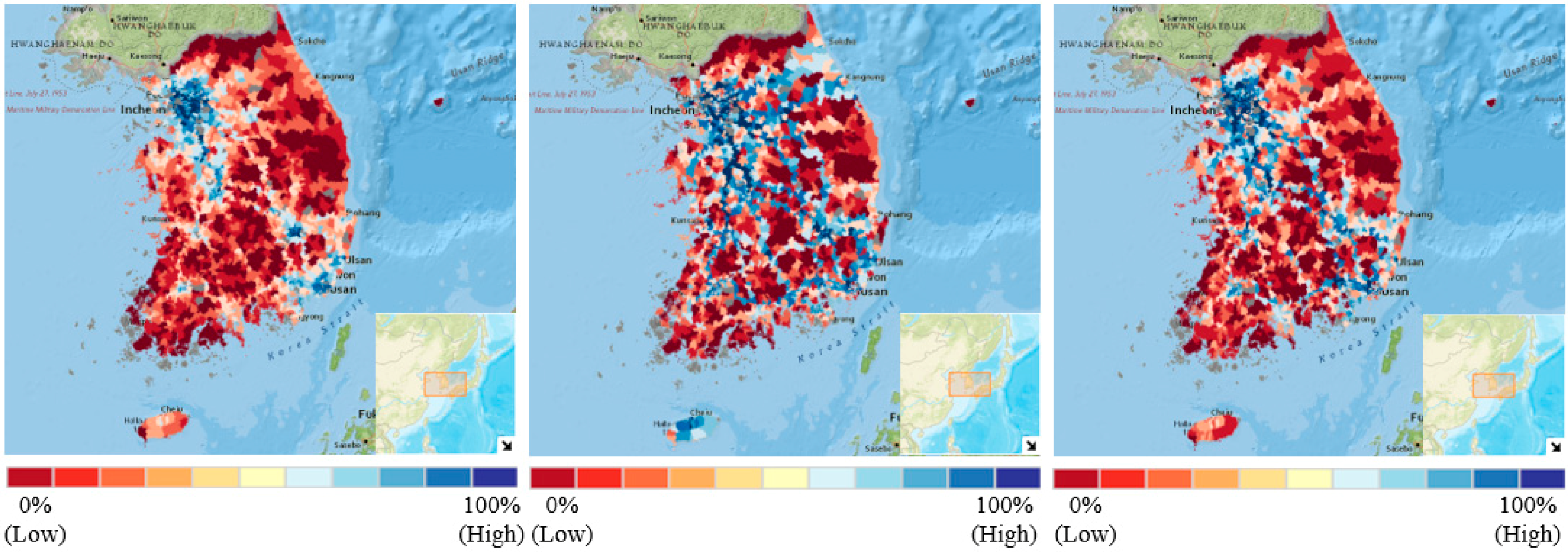
3.1.1. Dependent Variable: Traffic Volumes

The dependent variables in this study were traffic volumes measured as annual average daily traffic (AADT) in the number of vehicles per day (see Table 1). The traffic volume used in this study refers to the estimated number of vehicles traveling on the road predicted via an algorithm that estimates the traffic volume of unobserved roads using observed actual traffic volume and navigation data. The traffic data was at the finer level of geographical boundary in South Korea, which is Eup/Myeon/Dong (EMD). The sample size was around 3200. This study categorized traffic volume into three modes: truck, car, and bus, as they differ in size, speed, purpose, emissions, and impact on traffic. Consequently, three different models were generated for each variable in this investigation.

Table 1. Description and descriptive statistics of variables used in this study.

Variable	Description	Source	Mean	St. Dev
Dependent Variables (Target Features)
Truck	Log-transformed the amount of truck traffic in annual average daily traffic (AADT) in vehicles per day at the Eup/Myeon/Dong (EMD) level (dependent variable for the truck model)	KTI	6.595	1.030
Car	Log-transformed the amount of car traffic in annual average daily traffic (AADT) in vehicles per day at the EMD level (dependent variable for the car model)	KTI	8.038	1.108
Bus	Log-transformed the amount of bus traffic in annual average daily traffic (AADT) in vehicles per day at the EMD level (dependent variable for the bus model)	KTI	3.805	1.136
Independent Variables (Input Features)
Transportation Accessibility
Elementary	Log-transformed averaged travel time from each home to the nearest elementary school in minutes at the EMD level $Accessibilit{y}_j=\frac{{{\displaystyle \sum }}_{j_i\in {\Lambda }_i}\left(Po{p}_{j_i}\times Min\left(T_{j_i\to w}\right)\right)}{{{\displaystyle \sum }}_{j_i\in {\Lambda }_i}Po{p}_{j_i}}$ where $j$ is an EMD, $Po{p}_{j_i}$ denotes population size, and $T_{j_i\to W}$ represents aggregated travel time from the population-weighted centroid of EMD to the facility. The equation is from KTI.	KTI	1.388	0.473
Middle School	Log-transformed averaged travel time from each home to the nearest middle school in minutes at the EMD level	KTI	1.699	0.552
High School	Log-transformed averaged travel time from each home to the nearest high school in minutes at the EMD level	KTI	2.025	0.715
Mart	Log-transformed averaged travel time from each home to the nearest mart in minutes at the EMD level	KTI	2.570	0.962
Market	Log-transformed averaged travel time from each home to the nearest market in minutes at the EMD level	KTI	2.224	0.886
Bus Stop	Log-transformed averaged travel time from each home to the nearest bus stop in minutes at the EMD level	KTI	2.805	0.611
Transit Station	Log-transformed averaged travel time from each home to the nearest train station in minutes at the EMD level	KTI	3.010	0.740
Control Factors
Ave Speed	The log-transformed average speed of cars at the EMD level	KTI	3.539	0.357
Pop Density	The log-transformed population density in persons per km2 at the Si/Gun/Gu (SGG) level	SK	12.635	0.631
Emp Density	Log-transformed employment density in jobs per km2 at the SGG level	SK	11.776	0.564
Land Use Mix	Land use diversity index at the SGG level $land mix index=1-\left\{\frac{\left|\frac{r}{T}-\frac{1}{3}\right|+\left|\frac{c}{T}-\frac{1}{3}\right|+\left|\frac{o}{T}-\frac{1}{3}\right|}{4/3}\right\}$ where $r$ is areas of residential use permits in km2, $c$ is areas of commercial/industrial use permits in km2, $o$ is areas of other land use permits in km2, and $T$ is $r+c+o$ [17,18].	SK	0.572	0.138
Budget	Log-transformed total budgets in 10,000 Won at the SGG level	SK	13.811	0.582
Metro	1 if EMD is located in metropolitan areas, such as Seoul and Busan, 0 otherwise	NSDIP	0.328	0.470
Rural	1 if EMD is located in rural areas (Eup and Myeon), 0 otherwise	NSDIP	0.411	0.492

Abbreviation: Korea Transport Institute (KTI); Statistics Korea (SK); National Spatial Data Infrastructure Portal (NSDIP).

The data were collected from the Korea Transport Institute. The sources offer nationwide representative data and advantages of this research, including generalizability and reduced bias. Nationwide representative data sources provide a more comprehensive picture of the population and have the potential to boost the findings’ validity to be generalized to the full population of interest. The use of data sources that are representative of the entire country can help eliminate bias by ensuring that the sample is not systematically biased toward any particular groups or locations of the country. However, the data have limitations. For instance, nationwide analyses may not take into account specific regional or local contexts, which can limit the applicability of the findings to specific regions or populations. Also, nationwide data sources often have limited variables available for analysis, which can make it difficult to fully explore the relationships between different factors. Acknowledging the limitations, this study used the data sets.

Regarding the descriptive statistics, there was a difference in the traffic volumes that occurred between the three different modes of transportation. More specifically, the traffic volumes for automobiles were the largest, followed by trucks and buses. Figure 1 shows the spatial distribution of traffic volumes of the three modes. It shows a large concentration of traffic volumes in metropolitan regions, such as Seoul and Busan. In addition, the majority of the truck traffic was concentrated along the key highway corridors, such as the Gyeong-bu Line and the Ho-nam Line.

Figure 1. Spatial distribution of AADT of truck (Left), car (Middle), and bus (Right).

3.1.2. Independent Variables

This study used several independent variables categorized into two sections: (1) transportation accessibility, which is the focus of this study, and (2) control factors. First, this study employed diverse transportation accessibility indicators, including travel time to educational infrastructures (i.e., elementary school, middle school, and high school), commercial properties (i.e., mart and market), and public transportation infrastructures (i.e., bus stop and transit station). The models in this study were controlled for several factors that might be able to influence traffic volumes, such as population density, employment density, and land use diversity.

For the multicollinearity test, we developed ordinary least square (OLS) regression models for each truck, automobile, and bus, and estimated Variance Inflation Factor (VIF). The results of OLS models, which have adjusted R-squared of 0.485, 0.669, and 0.382 each for the three models, in Table 2 reveal that none of the independent variables show VIF of more than 10. Therefore, we concluded that the inclusion of all variables shown in Table 2 would not produce bias and issues related to the multicollinearity. Additionally, many of the variables show a significant relationship with traffic volumes of automobiles, buses, and trucks.

Table 2. Results of OLS regression models.

Variables	Truck		Car		Bus
	Estimates (p-Value)	VIF	Estimates	VIF	Estimates	VIF
Elementary	0.109 ** (0.027)	3.277	−0.016 (0.702)	3.277	0.010 (0.863)	3.277
Middle School	−0.072 * (0.079)	3.108	−0.018 (0.619)	2.108	−0.085 * 0.089)	2.108
High School	−0.183 *** (<0.001)	3.002	−0.182 *** (<0.001)	2.002	−0.193 *** (<0.001)	3.002
Mart	−0.405 *** (<0.001)	4.603	−0.418 *** (<0.001)	4.603	−0.535 *** (<0.001)	4.603
Market	−0.067 *** (0.008)	3.052	−0.107 *** (<0.001)	3.052	−0.022 (0.482)	3.052
Bus Stop	0.033 (0.193)	1.459	0.093 *** (<0.001)	1.459	−0.165 *** (<0.001)	1.459
Transit Station	−0.041 * (0.052)	1.440	−0.016 (0.385)	1.440	−0.045 * (0.078)	1.440
Ave Speed	0.916 *** (<0.001)	5.022	0.564 *** (<0.001)	5.022	1.824 *** (<0.001)	5.022
Pop Density	−0.339 *** (<0.001)	4.080	−0.303 *** (<0.001)	4.080	−0.391 *** (<0.001)	4.080
Emp Density	0.164 *** (<0.001)	4.226	0.122 *** (0.002)	4.226	0.182 *** (0.001)	4.226
Land Use Mix	−0.123 (0.219)	1.154	−0.170 ** (0.049)	1.154	0.005 (0.965)	1.154
Budget	0.435 *** (<0.001)	1.881	0.423 *** (<0.001)	1.881	0.386 *** (<0.001)	1.881
Metro	0.946 *** (<0.001)	2.925	1.063 *** (<0.001)	2.925	1.124 *** (<0.001)	2.925
Rural	−0.310 *** (<0.001)	5.116	−0.349 *** (<0.001)	5.116	−0.279 *** (<0.001)	5.116
Constant	1.137 * (0.069)		3.995 *** (<0.001)		−2.903 *** (<0.001)
Model Performance
Observation	3278		3278		3278
Adj. R squared	0.485		0.669		0.382

Significance level: * p < 0.1; ** p < 0.05; *** p < 0.01.

3.2. Methodological Approach

This study used the methodological approach depicted in Figure 2 to develop XGB models and SHAP values. The process can be categorized into several parts: (1) collect data, (2) split data into train and test sets, (3) train 5 machine learning algorithms with hyper-parameter tuning using the grid-search, (4) search for optimal algorithm using the 10-fold cross-validation, (5) employ SHAP method, and (6) interpret SHAP methods, including feature importance, summary plot, dependence plot, and interaction value plot. This study employed several Python packages, such as Sklearn.

Figure 2. Overall process of the methodological approach used in this study.

3.2.1. Extreme Gradient Boosting Decision Tree Model

This study used XGB. The algorithm is a type of gradient-boosting algorithm that uses decision trees as base learners [19]. It works by iteratively adding decision trees to the model, with each tree attempting to correct the errors made by the previous tree [20]. During training, XGB calculates the gradient and Hessian of the loss function concerning each prediction and then fits a decision tree to these values. The algorithm then adds this new tree to the model and updates the predictions for each sample based on the new tree’s output. This process is repeated for a specified number of iterations or until convergence is achieved. One key feature of XGB is its ability to handle missing data and regularization techniques such as L1 and L2 regularization. Additionally, it has built-in support for parallel processing and can handle large datasets efficiently [21]. Overall, XGB is a powerful machine-learning algorithm that has been shown to achieve state-of-the-art performance on a wide range of tasks [14].

XGB algorithm in this study is trained using a comprehensive shear strength database of 3278 samples, where 80% and 20% of the data are, respectively used for training and testing. The XGBoost algorithm contributes to the predictive model by achieving approximately 66.4%, 80.9%, and 54.3% validation accuracy for truck, car, and bus models, respectively, which exceeds the model performance of linear regression (LR), decision tree (DT), random forest (RF), and gradient boosting decision tree (GB) models (see Table 3). Therefore, we selected XGB as an optimal algorithm and interpreted it by using the Shapley value (SHAP).

Table 3. Model performance comparison.

Algorithms	Truck		Car		Bus
	R Squared	Explained Variance	R Squared	Explained Variance	R Squared	Explained Variance
LR	0.492	0.495	0.670	0.671	0.389	0.392
DT	0.534	0.536	0.710	0.711	0.403	0.405
RF	0.655	0.657	0.803	0.804	0.525	0.527
GB	0.662	0.663	0.807	0.809	0.538	0.539
XGB	0.664	0.666	0.809	0.810	0.543	0.545

Abbreviation: Linear regression (LR), decision tree (DT), random forest (RF), gradient boosting decision tree (GB), and extreme gradient boosting decision tree (XGB) models.

The hyper-parameters of the XGB truck model were an alpha of 0.01, a learning rate of 0.1, a max depth of 6, a number of estimators of 250, and a subsample of 0.9. Those of XGB car models were an alpha of 0.1, a learning rate of 0.1, a max depth of 6, a number of estimators of 250, and a subsample of 1.0. Finally, those of the XGB Bus model were an alpha of 0, a learning rate of 0.1, a max depth of 6, a number of estimators of 250, and a subsample of 0.8. In addition to the model specification of the XGB algorithm, the hyper-parameters of DT truck, car, and bus models were a max depth of 6, max features of auto, and a minimum sample leaf of 5. Also, after the grid search, RF truck, car, and bus models had a max depth of 10, minimum samples of 5, and a number of estimators of 250. Lastly, GB had a loss function of ls, a max depth of 6, max features of sqrt, and a number of estimators of 250.

The mathematical fundamentals will be introduced briefly in what follows. The equations are from several previous studies, such as Feng et al. [22] and Chen and Guestrin [23]. That is, we declared that we do not have the originality to develop the equations here. Considering we have a database including $n$ samples, say,

$$D\left\{\left(x_1,y_1\right),\left(x_2,y_2\right),\dots ,\left(x_n,y_n\right)\right\}$$

(1)

where $x_i, i=1,2,\dots ; n=$ input variables; $y_i=$ output variable. Thus, the task is to train a model to find the mapping between the inputs and output, say,

$${\widehat{y}}_i=\varphi \left(x_i\right)={\displaystyle \sum }_{k=1}^k{\alpha }_{k}f{f}_k\left(x_i\right)$$

(2)

where ${\widehat{y}}_i=$ prediction value $\varphi \left(·\right)$ final strong learner; $f_k\left(·\right)$ weak learner generated by the decision tree (DT) method; $K=$ number of weak learners; and ${\alpha }_k=$ learning rate used to avoid overfitting. According to XGBoost, a loss function $\mathcal{L}\left(·\right)$ is defined to represent the error between the prediction ${\widehat{y}}_i$ and the real value $y_i$, which has the following form:

$$\mathcal{L}\left(\varphi \right)={\displaystyle \sum }_{i}L\left(x_i,{\widehat{y}}_i\right)+{\displaystyle \sum }_k\mathsf{\Omega }\left(f_k\right)$$

(3)

in which the first right-hand-side term, $L\left(·\right)$, denotes realistic training loss between real and predicted values, and the second right-hand-side term, $\mathsf{\Omega }\left(·\right)$, denotes the complexity of the model, which is usually referred to as the regularization term. These two terms, respectively measure how well the model fits the data and the complexity of the model. In general, a squared loss function is adopted for the first term, whereas the second term is expressed by the tree node number and the L2 norm of the leaf score. That is,

$$L\left(x_i,{\widehat{y}}_i\right)={\left(y_i-{\widehat{y}}_i\right)}^2$$

(4)

$$\Omega \left(f_k\right)=\gamma T+\frac{1}{2}\lambda \parallel w_k\parallel$$

(5)

where $T=$ number of leaf nodes; $w_k=$ leaf scores (or weights); and $\gamma$ and $\lambda =$ penalty coefficients. Therefore, the problem becomes one of finding the appropriate learner $f_t$ at each step $t\le K$ to minimize the loss function, as in

$$f_t=arg\underset{f_t \in \mathcal{F}}{min}\mathcal{L}\left({\varphi }_t\right)=arg\underset{f_t \in \mathcal{F}}{min}\left[{\displaystyle \sum }_{i=1}^{n}L\left(y_i,{\varphi }_t\left(x_i\right)\right)+{\displaystyle \sum }_{k=1}^t\Omega \left(f_k\right)\right]$$

(6)

Here, at the $t$th step, the objective can be rewritten as

$$\mathcal{L}\left({\varphi }_t\right)={\displaystyle \sum }_{i=1}^{n}L\left(y_i,{\varphi }_t\left(x_i\right)\right)+{\displaystyle \sum }_{k=1}^t\Omega \left(f_k\right)={\displaystyle \sum }_{i=1}^{n}L\left(y_i,{\widehat{y}}_i^{t-1}+f_t\left(x_i\right)\right)+\Omega \left(f_t\right)+const.$$

(7)

where ${\widehat{y}}_i^{t-1}=$ predicted value at last step; and const. represents ${{\displaystyle \sum }}_{k=1}^{t-1}\Omega \left(f_t\right)$, which is indeed a constant.

Considering a second-order Taylor expansion and neglecting the constant term, the objective loss function in Equation (6) can be further approximated as

$$\mathcal{L}\left({\varphi }_t\right)\simeq {\displaystyle \sum }_{i=1}^n\left[L\left(y_i,{\widehat{y}}_i^{t-1}\right)+g_i{f}_t\left(x_i\right)+\frac{1}{2}{h}_i{f}_t^2\left(x_i\right)\right]+\Omega \left(f_t\right)$$

(8)

where $g_i={\partial }_{{\widehat{y}}_i^{t-1}}L\left(y_i,{\widehat{y}}_i^{t-1}\right)$ and $h_i={\partial }_{{\widehat{y}}_i^{t-1}}^{2}L\left(y_i,{\widehat{y}}_i^{t-1}\right)$ are the first and second-order gradients of the loss function. The term $L\left(y_i,{\widehat{y}}_i^{t-1}\right)$ is a constant, so it can be removed in the minimization process. Meanwhile, denoting the sample set of leaf $j$ by $I_j$, the objective can be simplified as

$$\begin{array}{l}\mathcal{L}\left({\varphi }_t\right)={\displaystyle {\displaystyle \sum }_{i=1}^n}\left[g_i{f}_i\left(x_i\right)+\frac{1}{2}{h}_i{f}_t^2\left(x_i\right)\right]+\Omega \left(f_t\right)={\displaystyle {\displaystyle \sum }_{j=1}^n}\left[\left({\displaystyle {\displaystyle \sum }_{i\in I_j}}{g}_i\right)w_j+\frac{1}{2}\left({\displaystyle {\displaystyle \sum }_{i\in I_j}}{h}_i+\lambda \right)w_j^2\right]+\gamma T\\ \hspace{1em}\hspace{1em}\hspace{1em}\hspace{1em}\hspace{1em}\hspace{1em}\hspace{1em}={\displaystyle {\displaystyle \sum }_{j=1}^n}\left[G_j{w}_j+\frac{1}{2}\left(H_j+\lambda \right)w_j^2\right]+\gamma T\end{array}$$

(9)

where $G_j={{\displaystyle \sum }}_{i=I_j}{g}_i$ and $H_j={{\displaystyle \sum }}_{i\in I_j}{h}_i$. With this loss function, the optimized weight $w_j^{*}$ for leaf $j$, as well as the tree structure score $L_{split}$ after splitting, can be derived to build a tree, that is,

$$w_j^{*}=-\frac{G_j}{H_j+\lambda },\hspace{1em}{\mathcal{L}}_{split}=\frac{1}{2}\left[\frac{G_L^2}{H_L+\lambda }+\frac{G_R^2}{H_R+\lambda }-\frac{{\left(G_L+G_R\right)}^2}{H_L+H_R\lambda }\right]-\lambda$$

(10)

where $G_L$, $G_R$, $H_L$ and $H_R$ are the first and second gradients of the left and right children after the split, respectively.

3.2.2. Interpretable Machine Learning: Shapley Value

The interpretability of machine learning projects is becoming an increasingly significant requirement, and as a result, there is a growing need to communicate the complicated outputs of model interpretation methodologies to non-technical stakeholders [24,25]. Therefore, this study attempted to not only develop XGB algorithms but also interpret them using SHAP values. SHAP values are built on a concept from cooperative game theory that is used to quantify the contribution of each feature in a machine learning model to the final prediction [26]. In the context of machine learning, the SHAP value can be used to explain the output of a model by attributing a portion of the prediction to each input feature [22]. That is, it is capable of producing feature attributes for a single instance and allows further understanding of the prediction behavior of the algorithm [27].

Therefore, this study used SHAP in four ways (see Figure 2): (1) calculate feature importance, (2) offer summary plots, (3) present dependence plots, and (4) describe interaction plots. First, it can estimate the feature importance of each feature. Specifically, it calculates the average marginal contribution of each feature across all possible subsets of features [28,29]. To calculate the Shapley value for a given feature, we consider all possible subsets of features that include that feature and calculate the difference in model output when that feature is included versus when it is not included. We then take the average of these differences across all possible subsets, weighting each subset by its size relative to the total number of subsets. Second, SHAP can produce several plots for direct interpretation [30]. For instance, the summary plot shows the impact of each feature on model output for a single sample, with features ordered by importance. Also, the dependence plot presents how the value of a single feature affects model output by capturing non-linear relationships while accounting for interactions with other features. Furthermore, the interaction value plot shows how pairs of features interact to affect model output, with each point representing a single sample.

The SHAP value, $g\left(x^{\prime }\right)$, can be defined as

$$g\left(x^{\prime }\right)={\phi }_0+{\displaystyle \sum }_{i=1}^M{\phi }_i{x}_i^{\prime }$$

(11)

where $x^{\prime }$ is the vector of simplified input variables that are obtained from the original input variables $x$ in the data set; $M$ is the number of features of the data set; ${\phi }_0$ is a constant when all inputs are null; and ${\phi }_i$ is the attribution value for each feature $i$. It is noted that the authors do not have the originality of the equation, rather they are collected from previous studies, including Feng et al. [22] and Lundberg and Lee [27].

4. Results

This section consists of three subsections: (1) feature importance and its corresponding summary plot, (2) dependence plots to show non-linear relationships, and (3) interaction value plots to reveal the interaction effects of two variables on the dependent variable. The SHAP methodology was used to produce all the results in this section, which were based on the final three XGB algorithms for AADT of trucks, automobiles, and buses.

We selected XGB algorithms for all three models based on the results shown in Table 3. Table 3 indicates that XGB showed a significantly higher prediction accuracy compared to LR, DT, RF, and GB. There was, however, a difference in the model performance of the three XGB variants. This could be because the set of factors explained car traffic better than the other two modes of transportation. Furthermore, while many other characteristics, such as industrial accessibility, can be associated with truck and bus traffic, the model did not account for all of them. As a result, there is a disparity in model performance. However, this may not fully explain the variation. Thus, further study is needed to explore this aspect.

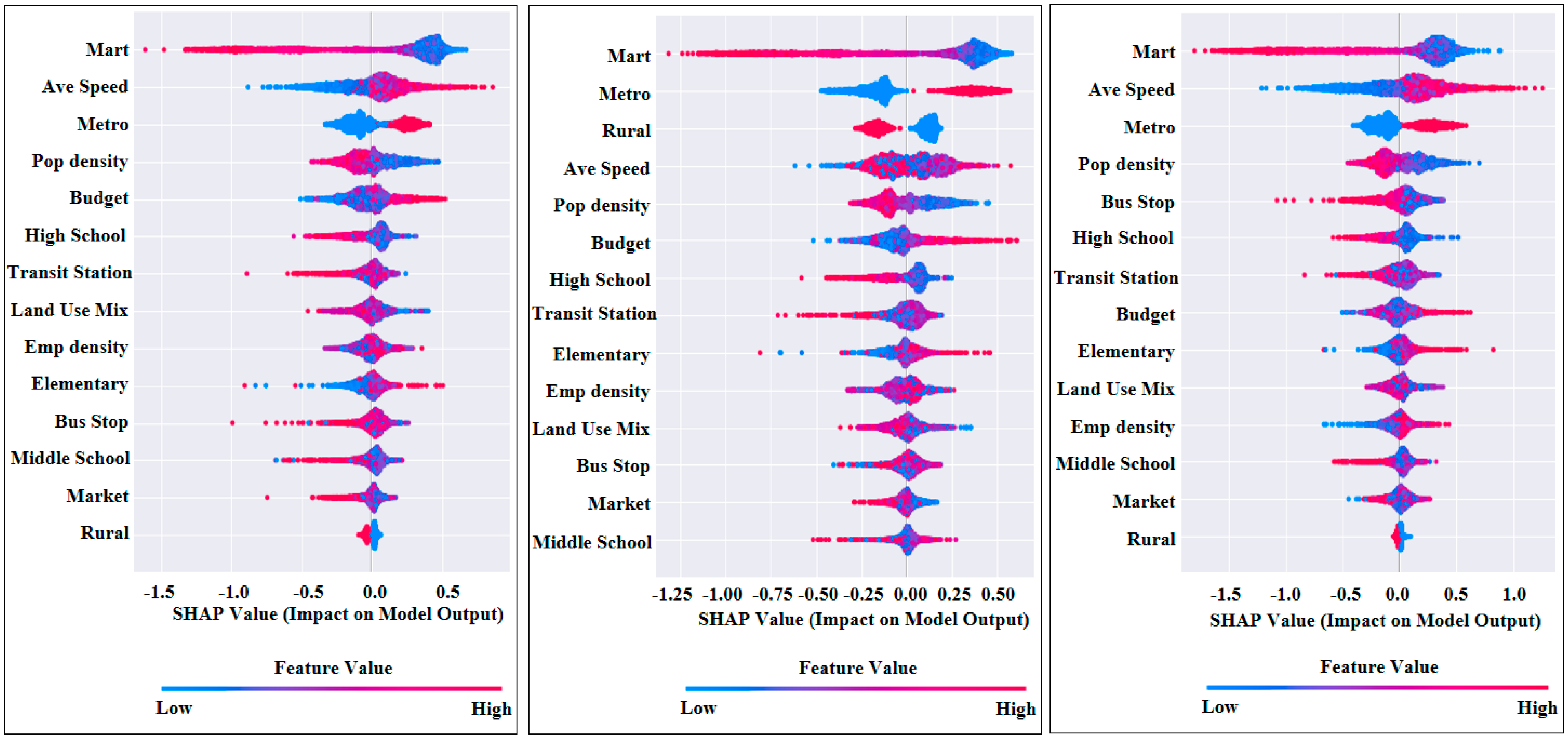
4.1. Feature Importance and Summary Plot

There are several methods for enhancing algorithm comprehension using SHAP, and feature importance is one of them. Feature importance allows us to estimate the contribution of each independent variable in percent to the model’s prediction. Table 4 shows the results of feature importance and its rank. According to the feature importance plot, the important features for predicting AADT of trucks were Mart (48.27%), Ave Speed (17.49%), Metro (15.85%), Pop Density (11.70%), and Budget (11.26%). A similar pattern was detected for car and bus models. Specifically, Mart, Metro, and Ave Speed showed a significant contribution when determining the AADT of car and bus. Like the spatial concentration of AADT of the transportation modes in Figure 1, Metro showed considerable feature importance in Table 4. Regarding the accessibility indicators, Bus Stop, Transit, and High showed approximately 10% feature importance when explaining the AADT of the bus. Other accessibility indicators exhibited around 5 to 10% of feature importance except for Mart.

Table 4. Results on feature importance of the truck, car, and bus models.

Variables	Truck		Car		Bus
	Mag.	Rank	Mag.	Rank	Mag.	Rank
Elementary	6.25%	10	6.16%	9	7.04%	9
Middle School	6.11%	12	3.80%	14	6.49%	12
High School	9.17%	6	8.44%	7	9.88%	6
Mart	48.27%	1	42.61%	1	46.22%	1
Market	5.19%	13	4.08%	13	6.15%	13
Bus Stop	6.12%	11	4.83%	12	11.70%	5
Transit Station	6.94%	7	6.92%	8	9.85%	7
Pop Density	11.70%	4	11.68%	5	15.57%	4
Emp Density	6.40%	9	6.15%	10	6.57%	11
Land Use Mix	6.58%	8	5.79%	11	6.81%	10
Budget	11.26%	5	10.44%	6	9.50%	8
Metro	15.85%	3	24.16%	2	19.75%	3
Rural	2.72%	14	14.07%	3	1.66%	14
Ave Speed	17.49%	2	13.49%	4	28.25%	2

The summary plot in Figure 3 adds the effects of independent variables to the feature importance in Table 4. Each point on the plot represents SHAP values for a feature and sample. While the y-axis shows each independent variable, the x-axis represents SHAP values. The color denotes the values of the independent variable, which ranges from low (red) to high (blue). Similar to the findings in Table 4, Figure 3 shows that the three most important features were Mart and Ave Speed for the truck model, Mart and Metro for the car model, and Mart and Ave Speed for the bus model. Moreover, the plots show lower values of Mart (i.e., closer to Mart) were associated with higher AADT for all three transportation modes in South Korea. Interestingly, lower accessibility to elementary school was associated with lower AADT of the transportation modes. Strict transportation regulations, such as the speed limit (30 km/h around the elementary school), may explain the results.

Figure 3. Summary plots for feature importance of the truck (Left), car (Middle), and bus (Right) models.

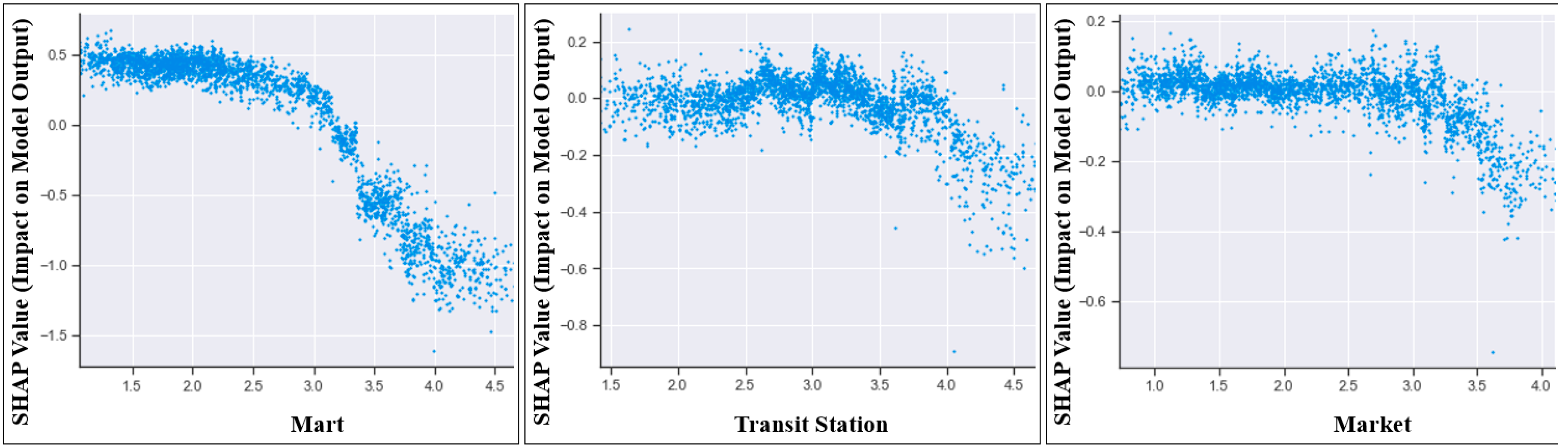
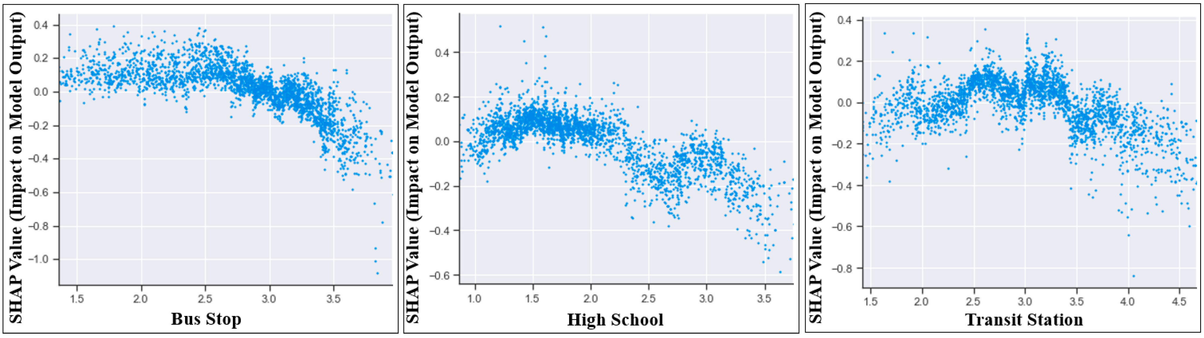
4.2. Dependence Plot

Figure 4, Figure 5 and Figure 6 show selected dependence plots for the important accessibility indicators. The plot gives a graphical description of the marginal effect of an independent variable on AADT, after accounting for the average influences of all other variables used in the XGB model [31]. One of the strengths of this method is that it is not constrained by the linearity assumption in the econometrics, rather it can reveal non-linear relationships [32]. In the plots in the figures, each sample of the dataset appears as its point, and the point is presented as a scatterplot of the value of an independent variable on the x-axis and its corresponding SHAP values on the y-axis.

Figure 4. Selected dependence plots of the truck model.

Figure 5. Selected dependence plots of the car model.

Figure 6. Selected dependence plots of the bus model.

In Figure 4, all else equal, the SHAP values for the accessibility index for Mart were comparable between 0 and 4, but then decreased sharply, meaning that better access to Mart showed a higher AADT of truck for a certain range, while AADT considerably decreased after the range. Also, accessibility to transit was comparable, whereas the plot exhibited a negative approximately linear trend after a certain point. Figure 5 demonstrates dependent plots that show the non-linear association between Mart, High, Transit, and AADT of cars. For accessibility to Mart (Mart), the AADT of cars was high when the travel time to high school was lower. However, AADT substantially decreased after the log-transformed travel time of 3. Also, the effect of accessibility to high school (High) did not change, but it reduced by more than 2.5 away from the high school. The effective range of accessibility to transit stations (Transit) on AADT of cars was between 2.5 and 3.5. Figure 6 shows the non-linear relationship between the AADT of bus and Bus Stop, High, and Transit. The AADT of buses was higher the closer they were to the bus stop, which is in line with the findings of earlier research and makes intuitive sense. Complex non-linear relationships were observed in High and Transit. Specifically, the effects of High and Transit were substantially large when the log-transformed travel times to high school and transit station were 1.5 and 2, respectively.

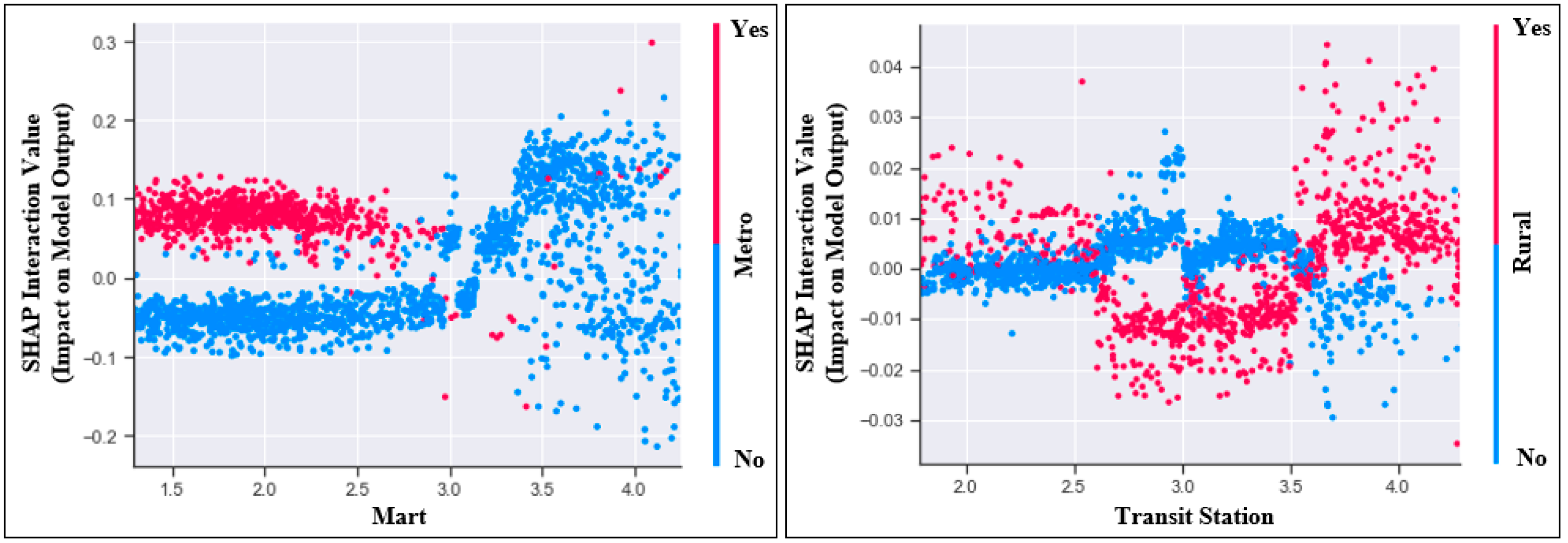
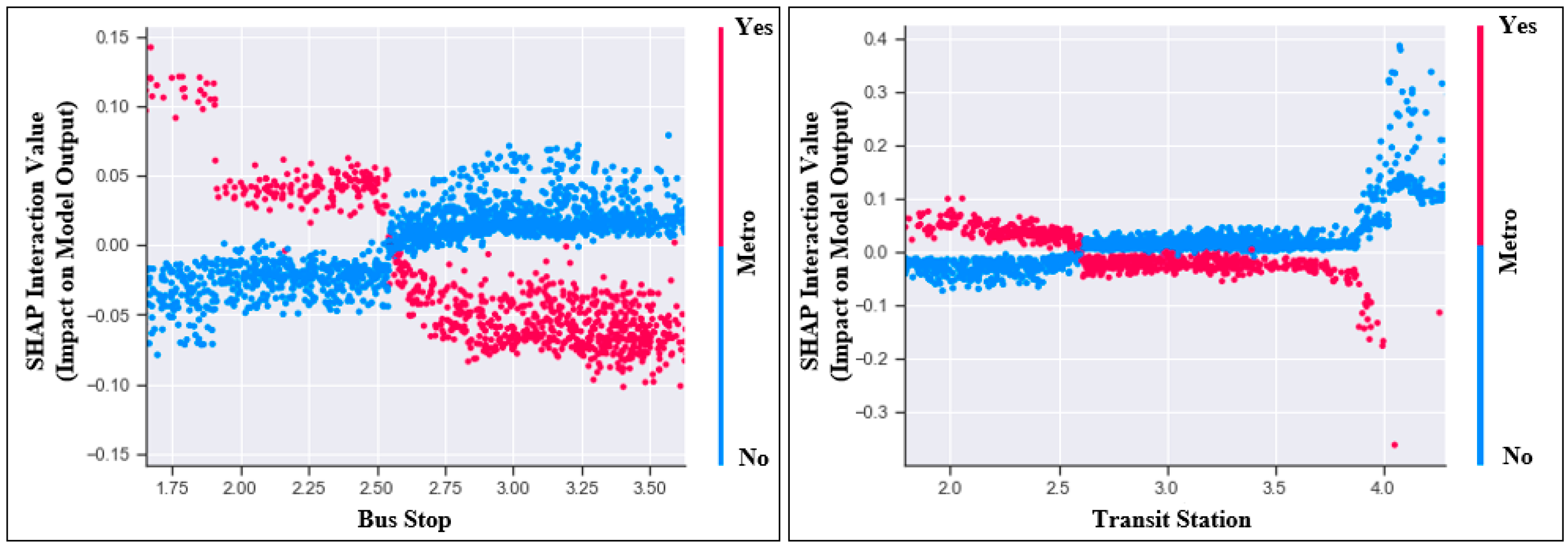
4.3. Interaction Value Plot

The interaction value plots in Figure 7, Figure 8 and Figure 9 visualize interaction effects between two independent variables on the AADT of the truck, car, and bus. Figure 7 demonstrates that controlling for the independent variables, the effect of accessibility to Mart in the metropolitan areas on AADT of trucks (red dots) was substantially larger than that in other areas (blue dots). Also, the interaction effect between Metro and Transit was the second degree in Figure 7, suggesting that while the lower or higher travel time to transit stations in rural areas was associated with higher AADT of trucks, the AADT of trucks reached the peak with medium travel time to the infrastructure in other areas. Figure 8 reveals that in the metropolitan areas, better accessibility to elementary school was associated with substantially lower AADT of cars. However, in other areas with lower car ownership and ridership, the direction of the association was the opposite. The interaction effects in Figure 9 were significant. Specifically, better accessibility to the bus stop or transit station particularly in metropolitan areas was associated with the AADT of buses, but the accessibility in other areas seems to have a nearly linear and positive influence on the AADT of buses.

Figure 7. Selected interaction value plots of the truck model.

Figure 8. Selected interaction value plots of the car model.

Figure 9. Selected interaction value plots of the bus model.

5. Discussion

5.1. Key Findings

There are several key findings in this study. First, accessibility indicators exhibited around 5 to 10% of feature importance except for Mart (around 50%). Also, the important features for predicting the AADT of trucks were Mart (48.27%), Ave Speed (17.49%), Metro (15.85%), Pop Density (11.70%), and Budget (11.26%). A similar pattern was detected for car and bus models. Second, the dependence plots indicated threshold effects. For instance, the SHAP values for the accessibility index for Mart were comparable between 0 and 4 but then decreased sharply, indicating that better access to Mart showed a higher AADT of trucks for a certain range, while AADT considerably decreased after the range. Third, this study found interaction effects in the interaction plots. For instance, better accessibility to public transportation infrastructures, such as bus stops and transit stations, was associated with higher annual average daily traffic (AADT), particularly in metropolitan areas including Seoul and Busan.

5.2. Implication

The results of this study indicate a significant and non-linear relationship between transportation accessibility indicators and traffic volumes. The findings of this study have important implications for transportation planning and policy. Specifically, they suggest that improving accessibility to public transportation infrastructures can help increase traffic volumes of buses, particularly in metropolitan areas, including Seoul and Busan, which can promote sustainable modes of transportation. Additionally, they suggest that increasing accessibility to large-scale marts may have unintended consequences on traffic volumes for both trucks and automobiles and induce congestion, which implies that it should be approached with caution. Interestingly, given that better accessibility to elementary schools was associated with lower AADT for all three transportation modes, strict transportation regulations, such as a speed limit of 30 km/h, may be an adequate approach to lower traffic volumes and congestion.

5.3. Limitation of this Study and Future Research Direction

This study has several limitations. First, the findings of this study may be limited to the specific area and transportation system examined in this study. The results may not necessarily apply to other areas or transportation systems with different characteristics. Second, the study relies on data from various sources, including traffic volume counts, transportation infrastructure maps, and demographic data. Some data may be incomplete or inaccurate, which could affect the results of the study. Third, the study examines the association between accessibility to infrastructures and traffic volumes but cannot establish causality. Other factors not examined in this study, such as land use patterns and travel behavior, may also influence traffic volumes. Fourth, the study examines traffic volumes over a specific time frame, and the relationship between accessibility to infrastructures and traffic volumes may vary over longer or shorter periods.

This study suggests several future research directions. For instance, further studies are needed to explore how transportation accessibility impacts traffic volumes within diverse regional or local contexts. Also, future study needs to expand diverse sets of accessibility indicators, such as accessibility to employment, and explore the associations.

6. Conclusions

This study aimed to explore the relationship between accessibility to infrastructures and traffic volumes across different modes of transportation in South Korea using XGB and SHAP approaches. We believe this research is an important step in understanding the complex relationship between accessibility to infrastructures and traffic volumes. By understanding the factors that influence traffic volumes, the study aims to provide important insights into how transportation systems can be developed and managed to meet the needs of users while also addressing social, economic, and environmental challenges [33]. The findings of this study have important implications for transportation planning and policy and highlight the need to consider accessibility to infrastructures when developing transportation plans and policies [10].

References

1. Arnott, R.; Small, K. The Economics of Traffic Congestion. Am. Sci. 1994, 82, 446–455. [Google Scholar]
2. Mondschein, A.; Taylor, B.D. Is traffic congestion overrated? Examining the highly variable effects of congestion on travel and accessibility. J. Transp. Geogr. 2017, 64, 65–76. [Google Scholar] [CrossRef]
3. Boarnet, M.G. A Broader Context for Land Use and Travel Behavior, and a Research Agenda. J. Am. Plan. Assoc. 2011, 77, 197–213. [Google Scholar] [CrossRef]
4. Ewing, R.; Cervero, R. Travel and the Built Environment. J. Am. Plan. Assoc. 2010, 76, 265–294. [Google Scholar] [CrossRef]
5. El-Assi, W.; Salah Mahmoud, M.; Nurul Habib, K. Effects of built environment and weather on bike sharing demand: A station level analysis of commercial bike sharing in Toronto. Transportation 2017, 44, 589–613. [Google Scholar] [CrossRef]
6. Ding, C.; Cao, X.; Wang, Y. Synergistic effects of the built environment and commuting programs on commute mode choice. Transp. Res. Part A Policy Pract. 2018, 118, 104–118. [Google Scholar] [CrossRef]
7. Guan, X.; Wang, D. Influences of the built environment on travel: A household-based perspective. Transp. Res. Part A: Policy Pract. 2019, 130, 710–724. [Google Scholar] [CrossRef]
8. Bai, S.; Jiao, J. Dockless E-scooter usage patterns and urban built Environments: A comparison study of Austin, TX, and Minneapolis, MN. Travel Behav. Soc. 2020, 20, 264–272. [Google Scholar] [CrossRef]
9. Frank, L.D.; Sallis, J.F.; Saelens, B.E.; Leary, L.; Cain, K.; Conway, T.L.; Hess, P.M. The development of a walkability index: Application to the Neighborhood Quality of Life Study. Br. J. Sports Med. 2010, 44, 924–933. [Google Scholar] [CrossRef]
10. Duranton, G.; Turner, M.A. Urban Growth and Transportation. Rev. Econ. Stud. 2012, 79, 1407–1440. [Google Scholar] [CrossRef]
11. Lavieri, P.S.; Dai, Q.; Bhat, C.R. Using virtual accessibility and physical accessibility as joint predictors of activity-travel behavior. Transp. Res. Part A Policy Pract. 2018, 118, 527–544. [Google Scholar] [CrossRef]
12. Wang, C.-H.; Chen, N.; Tian, G. Do accessibility and clustering affect active travel behavior in Salt Lake City? Transp. Res. Part D Transp. Environ. 2021, 90, 102655. [Google Scholar] [CrossRef]
13. Yan, X. Toward Accessibility-Based Planning: Addressing the Myth of Travel Cost Savings. J. Am. Plan. Assoc. 2021, 87, 409–423. [Google Scholar] [CrossRef]
14. Lee, S. Exploring Associations between Multimodality and Built Environment Characteristics in the U.S. Sustainability 2022, 14, 6629. [Google Scholar] [CrossRef]
15. Alzubi, J.; Nayyar, A.; Kumar, A. Machine Learning from Theory to Algorithms: An Overview. J. Phys. Conf. Ser. 2018, 1142, 012012. [Google Scholar] [CrossRef]
16. Bhavsar, P.; Safro, I.; Bouaynaya, N.; Polikar, R.; Dera, D. Machine Learning in Transportation Data Analytics. In Data Analytics for Intelligent Transportation Systems; Elsevier: Amsterdam, The Netherlands, 2017; pp. 283–307. ISBN 978-0-12-809715-1. [Google Scholar]
17. Bhat, C.R.; Gossen, R. A mixed multinomial logit model analysis of weekend recreational episode type choice. Transp. Res. Part B Methodol. 2004, 38, 767–787. [Google Scholar] [CrossRef]
18. Lee, S.; Wang, L. Intermediate Effect of the COVID-19 Pandemic on Prices of Housing near Light Rail Transit: A Case Study of the Portland Metropolitan Area. Sustainability 2022, 14, 9107. [Google Scholar] [CrossRef]
19. Lao, Y.; Qi, F.; Zhou, J.; Fang, X. A Prediction Method Based on Extreme Gradient Boosting Tree Model and its Application. J. Phys. Conf. Ser. 2021, 1995, 012017. [Google Scholar] [CrossRef]
20. Chang, Y.-C.; Chang, K.-H.; Wu, G.-J. Application of eXtreme gradient boosting trees in the construction of credit risk assessment models for financial institutions. Appl. Soft Comput. 2018, 73, 914–920. [Google Scholar] [CrossRef]
21. Liu, J.; Wang, B.; Xiao, L. Non-linear associations between built environment and active travel for working and shopping: An extreme gradient boosting approach. J. Transp. Geogr. 2021, 92, 103034. [Google Scholar] [CrossRef]
22. Feng, D.-C.; Wang, W.-J.; Mangalathu, S.; Taciroglu, E. Interpretable XGBoost-SHAP Machine-Learning Model for Shear Strength Prediction of Squat RC Walls. J. Struct. Eng. 2021, 147, 04021173. [Google Scholar] [CrossRef]
23. Chen, T.; Guestrin, C. XGBoost: A Scalable Tree Boosting System. In Proceedings of the 22nd ACM SIGKDD International Conference on Knowledge Discovery and Data Mining, San Francisco, CA, USA, 13–17 August 2016; Association for Computing Machinery: New York, NY, USA, 2016; pp. 785–794. [Google Scholar]
24. Bibal, A.; Frénay, B. Interpretability of Machine Learning Models and Representations: An Introduction. In Proceedings of the 24th European Symposium on Artificial Neural Networks ESANN, Bruges, Belgium, 27–29 April 2016; pp. 77–82. [Google Scholar]
25. Molnar, C. Interpretable Machine Learning: A Guide for Making Black Box Models Explainable; Leanpub: Victoria, BC, Canada, 2021. [Google Scholar]
26. Sundararajan, M.; Najmi, A. The Many Shapley Values for Model Explanation. In Proceedings of the 37th International Conference on Machine Learning, Vienna, Austria, 21 November 2020; pp. 9269–9278. [Google Scholar]
27. Lundberg, S.; Lee, S.-I. A Unified Approach to Interpreting Model Predictions. arXiv 2017, arXiv:1705.07874. [Google Scholar]
28. Rodríguez-Pérez, R.; Bajorath, J. Interpretation of machine learning models using shapley values: Application to compound potency and multi-target activity predictions. J. Comput. Aided Mol. Des. 2020, 34, 1013–1026. [Google Scholar] [CrossRef]
29. Ndichu, S.; Kim, S.; Ozawa, S.; Ban, T.; Takahashi, T.; Inoue, D. Detecting Web-Based Attacks with SHAP and Tree Ensemble Machine Learning Methods. Appl. Sci. 2022, 12, 60. [Google Scholar] [CrossRef]
30. Lundberg, S.M.; Erion, G.; Chen, H.; DeGrave, A.; Prutkin, J.M.; Nair, B.; Katz, R.; Himmelfarb, J.; Bansal, N.; Lee, S.-I. Explainable AI for Trees: From Local Explanations to Global Understanding. arXiv 2019, arXiv:1905.04610. [Google Scholar] [CrossRef] [PubMed]
31. Ding, C.; Cao, X.; Næss, P. Applying gradient boosting decision trees to examine non-linear effects of the built environment on driving distance in Oslo. Transp. Res. Part A Policy Pract. 2018, 110, 107–117. [Google Scholar] [CrossRef]
32. Molnar, C.; Freiesleben, T.; König, G.; Casalicchio, G.; Wright, M.N.; Bischl, B. Relating the Partial Dependence Plot and Permutation Feature Importance to the Data Generating Process. arXiv 2021, arXiv:2109.01433. [Google Scholar]
33. Papa, E. Transport and Mobility Planning; Parker, G., Ed.; Macmillan: London, UK, 2021; ISBN 978-1-352-01192-0. [Google Scholar]
Disclaimer/Publisher’s Note: The statements, opinions and data contained in all publications are solely those of the individual author(s) and contributor(s) and not of MDPI and/or the editor(s). MDPI and/or the editor(s) disclaim responsibility for any injury to people or property resulting from any ideas, methods, instructions or products referred to in the content.
Article Metrics
Citations
Article Access Statistics
Multiple requests from the same IP address are counted as one view.