Abstract
Space syntax is a set of theories and techniques for analysing urban settlements and buildings. Here, we propose a new approach to perform syntactic analyses that requires only the declaration in a computer program of the connections between axial lines or convex spaces using Prolog, a logic programming language concerned with artificial intelligence. With this new tool, we found that the deep tree nature of modern estates can be mitigated with a concentric structure similar to the famous Bororo village. In fact, Portela, a high-rise settlement near Lisbon (Portugal), is structured around a central open space (green park) equipped with noninterchangeable facilities (mall, sports centre and church), which are highly synchronised with the surrounding buildings (towers and blocks). The transpatial relations between housing estates and the central zone are maximised either by a distributive ringy network or by a smart grid of pedestrian paths. The result is a compact and integrated settlement with a strong identity and sense of belonging. Nevertheless, this kind of concentric dual system is potentially unstable, a problem that was minimised by forcing a clear opposition with a popular neighbourhood at Portela’s vicinity. With this case study, we show how logic programming is a useful tool to describe the patterns of discrete systems as social knowables due to its declarative nature. In fact, a Prolog program represents a certain amount of knowledge, namely, concerned with the structure of an urban settlement (or building), which could be used to answer queries about the social and economic consequences of certain spatial designs.
1. Introduction
Space syntax is a set of techniques for analysing urban settlements and buildings, and theories linking space and society founded on architecture, engineering, mathematics, sociology, anthropology, ethnography, linguistics, psychology, biology and computer science. It was developed originally by Bill Hillier, Julienne Hanson and colleagues at the Bartlett School of Architecture and Planning, University College of London (UCL), in the 1970s. Their innovative approach was condensed in three landmark books: The Social Logic of Space [1], Decoding Homes and Houses [2] and Space is the Machine: A Configurational Theory of Architecture [3].
An important contribution of space syntax is the study of urban form using discrete systems, that is, computer-aided recursive techniques based on elementary generators such as a pair of open and closed cells. Another key contribution is the concept of depth in urban systems and its relation with social phenomena like pedestrian movements or crime incidence, with a special focus on different uses of open spaces by inhabitants and strangers, men and women, old and young, adults and children, and so on ([3], pp. 146–152). In this scope, space syntax influenced and contributed to several projects, namely, the redesign of Trafalgar Square or the location of the Millennium Bridge, both in London. Thus, space syntax is a relevant and universal approach for spatial studies, namely, related with the understanding and intervention in public open spaces.
Space syntax is mainly concerned with the study of the relations between convex spaces. Convexity exists when straight lines can be drawn from any point in a space to any other point in it without going outside of the space itself ([1], pp. 97–98). In fact, convex rather that concave spaces stimulate social interaction in the sense that everyone sees everybody within that kind of space. Thus, the starting point of a syntactic analysis is typically a map of the fattest convex and open (or permeable) spaces that cover the settlement (or building) in question. Eventually, this framework can be represented by an axial map with the smallest set of straight lines that pass through all convex spaces or by a map of segments. Then, several syntactic measures can be computed to explore the connectivity between spaces and lines, or the angular deviation between segments, in order to evaluate the degree of asymmetry (or integration) and distributeness of each convex space/line/segment or whole system ([4], pp. 154–164).
Space syntax analyses are typically performed with DepthmapX version 0.8.0, a visual and spatial network analysis software developed by the Space Syntax Laboratory at the University College of London, United Kingdom. DepthmapX requires a convex/axial/segment map with the spatial configuration of the complex in question as the input, previously designed with computer-aided design (CAD) or geographic information system (GIS) ([4], pp. 167–169 and [5]). This preparatory task may be laborious and difficult, namely, for researchers from social and economic sciences, which limits the dissemination of space syntax techniques beyond architects and urban planners. Here, we propose a new approach to perform syntactic analyses that does not require a previous drawing, shape file, graph or adjacency matrix, but only the declaration in a logic programming script, written in Prolog, of the connections between the convex spaces or axial lines of a settlement (or building), using natural language.
This innovative approach aims to capture the essence of space syntax. In fact, Prolog is a logic programming language developed by Alain Colmerauer, Philippe Roussel, Robert Kowalski and colleagues between Montreal, Marseilles and Edinburgh in the 1970s [6] exactly to process natural languages. It uses logic to represent knowledge and uses deduction to solve problems by deriving logical consequences ([7], p. 38). A corollary of using logic to represent knowledge is that such knowledge can be understood declaratively. This kind of reasoning is embodied in space syntax when it represents spatial arrangements as a field of knowables, that is, as a system of possibilities governed by a simple and underlying system of concepts ([1], p. 66).
In fact, clump, concentric, estate and other syntactic processes defined in the book The Social Logic of Space are recursions of simple relations between open and closed primary cells ([1], p. 78). Prolog is recursive by construction too and uses relational clausal logic in a straightforward way to declare binary concepts like containment or adjacency, used to define the elementary generators of space syntax processes. Thus, the social (and economic) logic of space can, and ought to be, represented by a logic and declarative programming language such as Prolog.
This new way to perform syntactic analyses is innovative in the sense that it facilitates the description of settlements (or buildings) using, namely, grammar and recursions side by side with the computation of classic syntactic measures. As shown, it can even extend the DepthmapX scope by calculating relative ringiness. In practice, this approach is very different from existing methods because it explores the power of natural language to describe spatial structures using logic programming.
This article is organised in the following manner: In Section 2, we introduce the case study of Portela, a paradigmatic high-rise housing complex located near Lisbon (Portugal); in Section 3, we briefly describe the key concepts of logic programming and space syntax (with a focus on configuration, depth, integration and distributedness) and introduce Prolog grammar and predicates; the main results of the syntactic analysis of the Portela settlement, using the previously described methods, are presented in Section 4; a brief discussion about the concentric dualism found in Portela is provided in Section 5; finally, some conclusions and future developments are pointed out in Section 6.
The material in this article is complemented by a series of open-source computer programs stored on SWISH (https://swish.swi-prolog.org/, accessed on 19 July 2023), whose links are indicated in the following sections. SWISH is the on-line version for sharing of SWI-Prolog, a free and versatile implementation of the Prolog language developed by Jan Wielemaker and colleagues at the University of Amsterdam, Netherlands, since 1987 [8]. For convenience, those (and other) links were centralised in the Space Syntax with Prolog website: https://www.sswprolog.net/, accessed on 19 July 2023, which provides several resources concerned with logic programming applied to space syntax.
2. Case Study
Portela is a high-rise housing complex with 5103 dwellings ([9], pp. 27–29) and about 12,000 inhabitants ([10], p. 518) located in Sacavém—Loures municipality, near Olivais Norte, the most modern of the Lisbon’s neighbourhoods ([11], p. 140). Thus, Portela is located on the outskirts of Lisbon, which, at the time, was a low-value location, despite the views of the Tagus River. In fact, the estate’s surroundings were very deprived in urban terms, being home to several slums ([12], p. 6).
Like Olivais Norte, Portela was inspired by the Athens Charter in the sense that it is structured with the following elements ([9], pp. 16–20):
- Hierarchical system of roads: main distributive circulation roads, local access to housing estates with ‘cul-de-sacs’, parking zones and paths exclusive to pedestrians;
- Strict zoning: shopping centre (mall), church, schools and other facilities located in a single sector at the centre of the complex bordered by four residential sectors;
- Leisure zones, namely, a green central park (Jardim Almeida Garrett, Figure 1) equipped with sport facilities (swimming pool, tennis courts and football club).
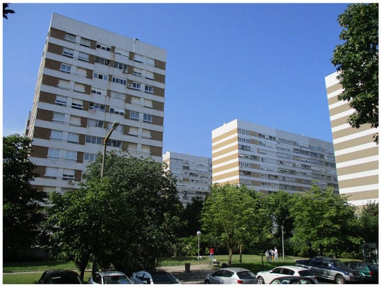 Figure 1. Perspective of Portela.
Planned during the 1950s and 1960s by architect Fernando Silva [1914–1983], Portela was built mainly during the 1970s after the approval of its master plan in 1969. It was developed by Manuel da Mota, a private entrepreneur, who almost doubled the number dwellings from the 2700 defined in the original plan, due to the informal manner of operating in the Portuguese real estate sector during the 1950s and 1960s ([10], pp. 520–521).
The development process was fragmented with the sale of the 196 plots by the developer to 134 contractors. Nevertheless, this process was guided rigorously by Fernando Silva with common rules in terms of architecture, layout and materials. This framework gave rise to a coherent and uniform complex, with a strong image and sense of belonging, particularly uncommon in Portuguese modern estates developed by private stakeholders, as stressed by Land et al. [13], p. 153:
“The variants derived from the orientation, sizing and levelling of the location of the various housing sectors, immediately lend it a plastic and urban interest which creates an intentionally uniform simplified concept architecture, which is enhanced by a convenient choice of qualities and chromatic variation of materials used. It was therefore following this concept that the layout of the buildings and of complementary works were connected and the projects with functional, technical and aesthetic characteristics were executed, and which all fit into the general and partial conception of the complex, infrastructures and furbishing in every aspect. Because uniformity is essential so that the aesthetic and functional level can be achieved within the corresponding budget, a spirit of cooperation is needed in everybody’s best interest, and the contractors therefore should respect the designs, details and specifications. The estate was developed following the Town Planning Regulation directives, created to ensure the required uniformity.”
Portela is considered a paradigm within Portuguese modern estates in part due to those aesthetic and functional qualities that can be found, typically, in public developments like Olivais Norte or Olivais Sul, rather than in private estates. In addition, Portela is also a paradigm because it successfully survived a set of high risk factors ([10], pp. 519–520). Firstly, Portela was built in a period (early 1970s) of international criticism to the modern high-rise model. Secondly, Portela dwellings were ready to be sold during the revolutionary period (1974–1975) with high hostility towards the private sector, fear of illegal occupations, high interest rates and massive influx of people coming from the Portuguese ex-colonies. Finally, the estate was promoted for the upper middle class, but it is located in a low-value location, as said.
Despite these negative factors, the majority of Portela’s inhabitants established in the 1970s still live there ([10], p. 521). This capacity of the settlement to retain its original residents, the sense of attachment expressed by most of them and the general social profile of its inhabitants explain the relative success of Portela in the universe of Portuguese large housing complexes ([10], p. 530).
3. Methods
3.1. Logic Programming
Logic programming deals with definitive clauses. Let be propositional variables or statements that can be true or false. A literal is a propositional variable or a negated propositional variable ([14], p. 269). A clause is a finite disjunction (logical connective ‘or’, noted by ∨) of literals. A Horn clause is a clause with at most one non-negated (positive) literal. Finally, a definite clause, also called a strict Horn clause, is a clause with exactly one non-negated (positive) literal. The disjunction form of a definite clause is
where q is the unique non-negated (positive) literal. We can write this kind of clause in the implication form
where ← means ‘if’ and ∧ is the conjunction connective ‘and’. Thus, if the literals are all true, then q is true. The part on the left side of Equation (2), before the ←, is called the head of the clause, the part on the right side is called the body ([15], p. 4). So, in general, if the body of the clause is true, then its head is true too. This fundamental deduction step is called modus ponens.
Logic programming uses modus ponens to compute the logical consequences of some set of definite clauses using a powerful inference rule called resolution ([16], pp. 21–22). Consider the following example:
The former clauses are related to each other by means of the literal ‘rectangle’, which occurs in the body of the first clause (a negative literal) and in the head of the second clause (a positive literal). Then, resolution will derive a third clause, called the resolvent, by eliminating this common literal, keeping all the other literals from both clauses. The output will be
That is, a square is a parallelogram with right angles and equal sides because a square is a rectangle with equal sides and a rectangle is a parallelogram with right angles.
This is the kind of inference that Prolog makes given a knowledge base (or database) of definite clauses that can express facts that are unconditionally true or rules that express conditions “if … then …” like the ones described above. The process of inference is called SLD-resolution with S for selection rule (from the left to the right of each clause), L for linear resolution (concerned with the shape of the proof trees obtained) and D for definitive clauses ([16], p. 44).
3.2. Basic Concepts
Based on graph theory and computer-aided simulations, space syntax aims to find and explain the relation between spatial configurations and social activities. Configuration is a concept that addresses the whole of a complex (settlement or building) rather than its parts and captures how the relations between two spaces, say A and B, might be affected by a third space C ([3], pp. 23–24). For instance, if A and B are adjacent or permeable, then they have a symmetric configuration in the sense that, if A is the neighbour of B, then B is the neighbour of A, as illustrated by the left-hand side of Figure 2.

Figure 2.
Basic configurations.
However, if only A is connected with a third space C, as in the right-hand side of the same figure, A and B become asymmetrical in relation with C because we have to pass through A to get to B from C, but we do not have to pass through B to get to A from C. Thus, asymmetry relates to depth, that is, with the number of spaces (or steps) necessary to go from a certain space, say C, to another space, A (1 step), B (2 steps), and so on.
If we count the number of steps necessary to go from a certain space to every other space in a complex, we can obtain a measure of its total depth (TD), or mean depth (MD) by dividing that total by the number of spaces in the complex minus one, the original space ([1], p. 108) ([2], pp. 27–28). In the previous example, the total depth of C is 3, which is the sum of steps to reach A and B (1 + 2) from that origin. This is also the case of B, but the total depth of A is 2, noting that this (central) space is directly connected with either B or C spaces (1 + 1). Thus, the mean depth is 1 (2/2) for A and 1.5 (3/2) for either B or C, noting that the number of spaces minus one in this simple complex is 2 (3 − 1).
This simple illustration suggests that syntactic measures can be computed for every (convex) space in a settlement or building. Then, we may eventually find that some spaces have a lower depth than all other spaces (A in the same example), and others have a greater depth (B and C). The former are the most integrated spaces, where social life and/or economic activities such as retail might be concentrated in cities ([4], p. 162), or the living room in most houses ([1], pp. 155–158) ([2], pp. 104–105) ([3], pp. 25–27). The latter are typically the most segregated, quiet or remote spaces in a town, building or house. Thus, integration is inversely related with depth. It is a global measure in the sense that it considers the configuration of a certain space in relation with all other spaces (or with spaces at a radius of n steps from the original space). In addition, local measures such as control are based on the relations between each space and only the spaces directly connected to it ([5], p. 14).
As an intelligent critique of modernism, space syntax stresses the deep tree-like configuration of modern estates ([1], pp. 129–132, 262–263). Firstly, the modern city is structured around a hierarchical street system, eventually composed by Le Corbusier’s seven roads types ([17], p. 157). Secondly, the number of spaces between each dwelling and the closest main street may be amplified by walls, stairs, galleries and other physical boundaries that are common in modern estates ([18], pp. 52–53), and by the number of stories in high-rise complexes. In fact, the modern dwelling is conceptually a space of retreat such as a monk cell. To get there, we might take a deep initiatory path like the one took by Le Corbusier himself, daily, to his flat in Paris (24 N.C.):
Le Corbusier’s apartment is a maisonnette. It can be accessed from the outside gallery which overhangs the small courtyard; from this gallery, the visitor either take the service lift or follow the spiral staircase connecting the seventh floor to the lower landing, where the main lift stops. This rather complicated procedure requires a real initiation ceremony to reach Le Corbusier’s apartment ([19], p. 36).
Thus, the configuration of a modern city is typically a deep tree. A tree is a special kind of graph, which contains a root such that there is a unique path from the root to any other node ([16], p. 83). Thus, trees are necessarily noncyclic or acyclic, that is, they do not contain paths from a node to itself. The absence of ‘rings’ in trees give them a non-distributed rather than a distributed configuration where there is more than one independent route from one space to another, including one passing through a third space ([1], p. 148). Distributedness can be illustrated by a recursive discrete process, where a primary cell or syntactic type is ‘glued’ together with cells of the same type by the space ‘between’ them, meaning that the global structure of the settlement is distributed amongst all primary cells ([1], p. 11).
3.3. Grammar
Among several influences, space syntax was founded on anthropology, namely, on the works of Claude Lévi-Strauss, Robert Sutherland, Bronislaw Malinowski and Franz Boas [1,3]. In addition, anthropology was influenced by structural analysis, namely, by the seminal works of the prince N. S. Troubetzkoy [20] on phonology. As stressed by Levi-Strauss ([21], pp. 31, 33):
Linguistic occupies a special place among the social sciences, to whose ranks it unquestionably belongs. It is not a social science like the others, but, rather, the one in which by far the greatest progress has been made. It is probably the only one which can truly claim to be a science, and which was achieved both the formulation of an empirical method and an understanding of the nature of the data submitted to its analysis. (…) Structural linguistics will certainly play the same role with respect to the social sciences that nuclear physics, for example, had played for the physical sciences.
Originally, Prolog was developed exactly to process natural languages, namely, French, using linear resolution on definitive clauses ([6], pp. 2, 6). Within this scope, the syntax of a language is specified by a grammar, which is a set of rules of the form ([16], p. 134):
sentence --> noun_phrase,verb_phrase.
noun_phrase --> article,noun.
verb_phrase --> verb,noun_phrase.
The former chunk states that a sentence may consist of a noun phrase followed by a verb phrase, with the former composed of an article and a noun and the later by a (transitive) verb and another noun phrase.
This kind of (structural) grammatical analysis can be applied directly to spatial problems, namely, to describe concentric villages like Bororo ([21], p. 141), Figure 3. Here, a large amount of convex space is invested in a central zone, which is highly synchronised with a large number of objects placed at its periphery ([1], pp. 92–93). This kind of concentric structure was found in many places, namely, in the village of Omarakana, the Trobriand Islands, Melanesia ([22], Figure I, p. 649).
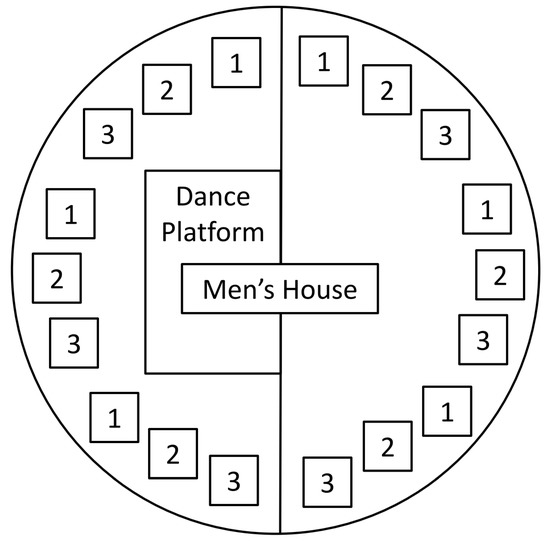
Figure 3.
Schematic plan of the Bororo village (1/2/3 is upper/middle/low class houses).
In fact, we can define a generic concentric village as a centre surrounded by a periphery where the former is composed of facilities and open spaces and the latter by several (up to three) types of housing estates, namely:
conc_village --> centre,periphery.
centre --> facility,open_space.
centre --> facility,facility,open_space.
centre --> facility,facility,open_space,open_space.
periphery --> housing.
periphery --> housing,housing.
periphery --> housing,housing,housing.
Then, we have to specify the terminal categories, such as words in a phrase, for the spaces that structure the Bororo village described in Figure 3:
facility --> [men_house].
facility --> [dance_platform].
open_space --> [scrub_land].
housing --> [upper_class_houses].
housing --> [middle_class_houses].
housing --> [low_class_houses].
After consulting this Prolog program (https://swish.swi-prolog.org/p/concentric_bororo.pl, accessed on 19 July 2023), we can ask the query
?-conc_village([men_house,dance_platform,scrub_land,
upper_class_houses,middle_class_houses,
low_class_houses],[]).
to get an affirmative answer, that is, the Bororo village respects the above-defined syntax of concentric villages because it is structured around a centre with two facilities (men’s house and dance floor) and an open space (scrub land) surrounded by three types of houses for upper, middle and low classes (respectively, 1, 2 and 3 in the same figure).
As stressed by Lévi-Strauss ([21], pp. 151–152), the concentric dualism found in Bororo masks a triad because it is not self-sufficient and its frame of reference is always the environment: ‘the opposition between cleared ground (central circle) and waste land (peripheral circle) demands a third element, brush or forest, that is, virgin land, which circumscribes the binary whole at same time extending it’.
3.4. Syntactic Measures
3.4.1. Knowledge Base
A Prolog program is a knowledge base, or database, composed of a collection of facts and rules, which describe a set of relations of interest [15]. Facts express unconditional truths ([16], p. 5), namely, the connections between lines in an axial map (the longest and fewest lines that cover the street grid) or between spaces in a convex map ([1], pp. 91–92) ([3], p. 98).
In Portela’s axial map (Figure 4), from left to right and top to bottom, we know that the west side of Avenida dos Descobrimentos is directly connected with 10 lines: Avenida da República, Rua Fernão de Magalhães, Rua Gonçalves Zarco, Rua Pedro Álvares Cabral, Rua Bartolomeu Dias, Rua Diogo Cão, Rua Infante Dom Henrique, Avenida dos Descobrimentos (south side) and two local circulations. These facts can be declared in a Prolog program (https://swish.swi-prolog.org/p/portela.pl, accessed on 19 July 2023) with the following:
connected(av_descobrimentos_W,av_republica,1).
connected(av_descobrimentos_W,rua_fernao_magalhaes,1).
connected(av_descobrimentos_W,rua_gonc_zarco,1).
connected(av_descobrimentos_W,rua_pedro_alvares_cabral,1).
connected(av_descobrimentos_W,rua_bartolomeu_dias,1).
connected(av_descobrimentos_W,rua_diogo_cao,1).
connected(av_descobrimentos_W,rua_inf_dom_henrique,1).
connected(av_descobrimentos_W,av_descobrimentos_S,1).
connected(av_descobrimentos_W,circ_NW,1).
connected(av_descobrimentos_W,circ_SW,1).
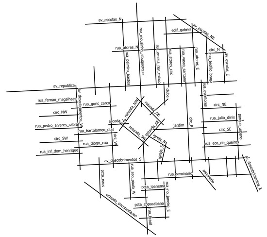
Figure 4.
Axial map of Portela.
These 10 clauses or atoms belong to the same predicate because they have the same name (‘connected’) and the same arity, that is, the same number of arguments (three) enclosed in parentheses and separated by commas ([16], pp. 25, 31). Here, the third argument is the topological distance between two adjacent lines, that is, one. In some applications, it may be greater than one in order to incorporate the metric distance or other cost (e.g., stairs or ramps) between two convex spaces [23], but here we adopt the topological distance introduced in The Social Logic of Space ([1], p. 103).
Clauses of the same predicate must be declared jointly in a Prolog program, so we must add the remaining connections concerned with the Portela’s axial map (Figure 4) in our knowledge base in order to proceed, namely:
connected(av_republica,pcta_jose_relvas,1).
connected(av_republica,circ_W,1).
connected(av_republica,rua_palmira_bastos,1).
…
connected(av_descobrimentos_S,pcta_sto_antonio,1).
Then, after consulting this program (https://swish.swi-prolog.org/p/portela.pl, accessed on 19 July 2023), we may ask it about the lines Y connected, for instance, with the west side of Avenida dos Descobrimentos by posing the query:
?-connected(av_descobrimentos_W,Y,1).
where the prefix ‘?-’ indicates that this is a query rather than a fact. In Prolog, a variable such as Y is written as a sequence of letters and digits, beginning with a capital letter or underscore. An answer to the previous query, e.g., Avenida da República, will be written {Y -> av_republica} following the notation of Flach ([16], p. 5). This means that Prolog found a value for the variable Y, that is, a solution given the knowledge base previously loaded and consulted. If asked, Prolog will try to find more values to Y given the knowledge base, namely, {Y -> rua_fernao_magalhaes}, {Y -> rua_gonc_zarco} and so on. These are the axial lines 1 step away from the west side of Avenida dos Descobrimentos, that is, at a depth of 1 from this particular root.
3.4.2. Connectivity
For practical purposes, we must create a pair of rules, that is, of conditional truths that can only be drawn when their premises are known to be true ([16], p. 5), which isolate the lines that are adjacent with a certain axis X in the sense that it can be connected with Y or, conversely, Y can be connected with X:
adjacent(X,Y,1):-connected(X,Y,1).
adjacent(X,Y,1):-connected(Y,X,1).
where the symbol: ‘-’ should be read as ‘if’. These rules mean ‘for any values of X and Y, X and Y are adjacent if X is directly connected with Y or Y is directly connected with X with topological distance 1’.
Now, we can compute the axial connectivity (AC) of some line, which is the number of other lines it intersects ([1], p. 103), using the SWI-Prolog [8] built-in predicate aggregate_all in order to count the number of adjacent lines:
connectivity(X,Y,AC):-aggregate_all(count,adjacent(X,Y,1),AC).
For instance, the following query returns {AC -> 10} because the west side of Avenida dos Descobrimentos is directly connected with 10 axial lines, as said:
?-connectivity(av_descobrimentos_W,Y,AC).
3.4.3. Control
Connectivity is the basic syntactic measure in the sense that others are based on it ([4], p. 158). In particular, the measure of control (E) proposed by Hillier and Hanson ([1], p. 109) and implemented below sums up the space denoted G to some space X by its immediate (adjacent) neighbours Z, where G is the reciprocal of the axial connectivity (AC) of each Z and the comma ‘,’ between predicates should be read as ‘and’:
control(X,Y,E):-aggregate_all(sum(G),(adjacent(X,Z,1),
connectivity(Z,Y,AC),G is 1/AC),E).
This specific rule illustrates how Prolog can be very useful and pedagogical in describing the syntactic concepts. In fact, it suggests the direct relation of control with the original line’s connectivity, that is, with the number of its adjacent neighbours, and the inverse relation with the connectivity of the last ones. In fact, spaces with a strong control, that is, with an E greater than 1, are typically connected with several spaces, namely, ‘cul-de-sacs’ or streets with few connections. Therefore, in order to be controlling, a line must see many spaces, but these spaces should each see relatively little ([5], p. 16).
3.4.4. Depth
Control is a local measure, since it only considers relations between a space and its immediate neighbours ([1], p. 109). Another local measure, controllability picks out areas that may be easily visually dominated ([5], p. 16). It is simply the ratio of connectivity to the total number of spaces 1 or 2 steps away from the original space. In order to compute this measure and the relative asymmetry, which is a global measure that considers the distance from a certain space to the others, we must first define a predicate for depth.
Obviously, axial connectivity is related with the concept of depth 1 in the sense that it is the number of lines 1 step away from the original line. In fact, we can define a rule such that Y is 1 deep from X if X and Y are adjacent:
depth(X,Y,1):-adjacent(X,Y,1).
Similarly, the lines 2 steps away from the original line are 1 step away from the lines adjacent to the root. The following rule explores this recursive nature of depth, that is, the spaces at depth 2 from X are the spaces Y at depth 1 from the spaces Z adjacent to X:
depth(X,Y,2):-adjacent(X,Z,1),depth(Z,Y,1),dif(X,Y).
where the SWI-Prolog [8] built-in predicate dif introduces a constraint that is true if and only if the 2-deep line Y is different from the original line X in order to avoid backward relations. The following query returns a list, denoted with square brackets ‘[Y]’, with the lines 2 steps away from the west side of Avenida dos Descobrimentos:
?-distinct([Y],(depth(av_descobrimentos_W,Y,2))).
where the built-in predicate distinct assures that no previous solution of the second argument bound the list [Y] to the same value. In practice, this useful predicate eliminates the same answer twice. For example, 2-deep lines like Rua Palmira Bastos that can be accessed through two or more lines directly connected with the original space, the west side of Avenida dos Descobrimentos, are included once in the list [Y]. Depth 3 can be defined in the same recursive way by isolating the spaces 2 steps away from the spaces Z directly connected with the original space X, depth 4 by isolating the deep 3 spaces, and so on:
depth(X,Y,3):-adjacent(X,Z,1),depth(Z,Y,2),dif(X,Y).
depth(X,Y,4):-adjacent(X,Z,1),depth(Z,Y,3),dif(X,Y).
…
3.4.5. Justified Graph
It is important to note that a space or line may be accessible at several steps from the same origin. For instance, Rua Gonçalves Zarco is either 1 step away from the west side of Avenida dos Descobrimentos or 3 steps away because we can pass through Avenida da República and the west circulation (pedestrian path circ_W, see Figure 4) to get there. This occurs in every axial map with ‘rings’ or ‘islands’. Therefore, we must create a new rule to fix the minimum number of steps D to go from X to Y once again using the Prolog’s predicate distinct that eliminates duplicated answers as described in the previous section:
graph(X,Y,D):-distinct([Y],depth(X,Y,D)).
We named this predicate ‘graph’ because it analytically generates the justified graph, or j-graph, for some root X. The resulting j-graph is a ‘picture’ with the depth of all spaces in a complex from a point on it ([3], pp. 22–23, 72–73). For instance, we can analytically describe the j-graph of the west side of Avenida dos Descobrimentos with the following query:
?-graph(av_descobrimentos_W,Y,D).
to obtain:
{Y -> av_republica, D -> 1}
{Y -> rua_fernao_magalhaes, D -> 1}
…
{Y -> pcta_jose_relvas, D -> 2}
{Y -> circ_W, D -> 2}
…
{Y -> rua_rio_janeiro_E, D -> 4}
3.4.6. Controllability
As suggested by the flowchart in Figure 5, the predicates graph (defined in the previous section) and connectivity (defined in Section 3.4.2) are the ‘building blocks’ to compute several measures, namely, the above-mentioned controllability (F) using the following code:
controllability(X,Y,Z,F):-connectivity(X,Y,AC),
aggregate_all(count, graph(X,Z,2), D2),
F is AC/(AC+D2).
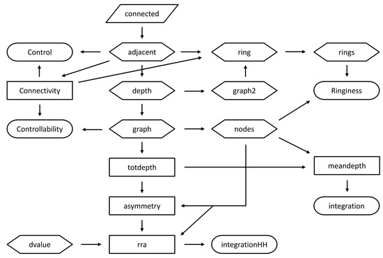
Figure 5.
Flowchart of Prolog predicates for space syntax.
3.4.7. Mean Depth
Another measure that can be computed with graph from Section 3.4.5 is mean depth (MD) referred to in Section 3.2. It is calculated by summing up the depth values D from a certain root X and dividing by the number of spaces (lines) in the complex minus one ([1], p. 108). The following implementation introduces two previous (auxiliary) predicates that compute the total depth (TD) and the number of nodes (N) in the complex except the root X:
totdepth(X,Y,TD):-aggregate_all(sum(D),graph(X,Y,D),TD).
nodes(X,Y,D,N):-aggregate_all(count,graph(X,Y,D),N).
meandepth(X,Y,D,MD):-totdepth(X,Y,TD),nodes(X,Y,D,N), MD is TD/N.
Mean depth is an important syntactic measure and its reciprocal can be used as a simple measure of the integration of each space in a complex as suggested by Heitor and Pinelo Silva [4], p. 162):
integration(X,Y,D,I):-meandepth(X,Y,D,MD), I is 1/MD.
3.4.8. Relative Asymmetry
The value of the total or (even) mean depth can be affected by the number of nodes in a graph. Thus, Hillier and Hanson ([1], p. 108) proposed a normalisation of MD, which eliminates the bias due to the number of nodes, that is:
asymmetry(X,Y,D,RA):-totdepth(X,Y,TD),nodes(X,Y,D,N),
RA is 2*(TD/N-1)/(N-1).
This formula will give a value between 0 and 1, with low values indicating a space that tends to integrate the whole complex or system, and high values for a space that tends to be segregated from the system. Thus, relative asymmetry (RA), also denoted by ‘i-value’ ([3], p. 77), is a normalised measure of integration. The Prolog program (https://swish.swi-prolog.org/p/portela.pl, accessed on 19 July 2023) for Portela has additional predicates to compute radius-r integration and other local measures.
3.4.9. Real Relative Asymmetry
The RA measure can be used to compare different systems with (approximately) the same number of spaces/lines. However, if the systems differ considerably in size, a second normalisation should be applied because a small system always looks more integrated than a large one ([5], p. 14).
To deal with this empirical problem, Hillier and Hanson ([1], pp. 109–113) proposed a second standardised measure, the real relative asymmetry (RRA), which is the RA value of the space divided by the RA value of the root of a graph shaped like a ‘diamond’ where there are k nodes at middle level, at one level above and below the middle level, at one level above and below the level, and so on until there is one node at the root and deepest nodes ([24], pp. 350–351). The following implementation uses the formula proposed by Kruger and Vieira ([25], p. 200) to estimate the RA value of the root of that diamond (d-value):
dvalue(K,DV):-DV is 2*(K*(log((K+2)/3)/log(2)−1)+1)/((K−1)*(K−2)).
rra(X,Y,D,RRA):-asymmetry(X,Y,D,RA),nodes(X,Y,D,N),dvalue(N+1,DV),
RRA is RA/DV.
The inverse of RRA is itself a measure of integration (IHH), the so-called ‘Hillier and Hanson (integration value with) d-value normalisation’ ([5], p. 25) that ‘captures the extent to which each spatial element contributes to drawing the whole configuration together into a more or less direct relationship’ ([2], p. 27):
integrationHH(X,Y,D,IHH):-rra(X,Y,D,RRA), IHH is 1/RRA.
3.4.10. Relative Ringiness
RA and RRA are measures of asymmetry. In addition, distributedness can be evaluated using either control (or controllability) or relative ringiness (RR). The RR of some space is the number of independent rings that pass through that space over the maximum that can pass through it, which will be the total number of nodes in the system minus one ([1], pp. 153–154). Detecting the number of rings that pass through some space is a very difficult task to be performed by a computer: for instance, the software DepthmapX 0.8.0 does not compute RR. As a programming language concerned with artificial intelligence, Prolog can do the task relatively well in most cases. In fact, the following code will produce accurate estimates for RR, namely, where the number of independent rings is lesser than axial connectivity:
graph2(X,Y,D):-distinct([Y],(depth(X,Y,D),D>1)).
ring(X,Y,Z,D):-adjacent(X,Y,1),graph2(Y,X,D),connectivity(X,Z,AC),
AC > 1.
rings(X,Y,Z,D,R):-aggregate_all(count,(ring(X,Y,Z,D)),C),
R is max(C-1,0).
ringiness(X,Y,Z,RR):-rings(X,Y,Z,D,R),nodes(X,Y,D,N), RR is R/N.
3.5. Workflow
It is quite easy to adapt the previous Prolog program to perform a swift analysis of another settlement or building, for example, the well-known farmhouse ‘La Bataille’ (Normandy, France) described by Hanson ([2], p. 85). Here are the practical steps:
- 1.
- Go to the SWI-Prolog [8] homepage: https://www.swi-prolog.org/;
- 2.
- Select ‘Try SWI-Prolog online (SWISH)’; alternatively, you can download and install SWI-Prolog [8] in your computer;
- 3.
- In the search box from the SWISH platform, find the portela.pl program and pick it in the pull-down call-out; if you have problems with the search function from SWISH, you can go directly to the web page: https://swish.swi-prolog.org/p/portela.pl, accessed on 19 July 2023;
- 4.
- At the top of this program (eventually downloaded with ‘File’-‘Download’, if you installed SWI-Prolog on your computer), you will find a knowledge base with the connections for Portela; please edit them to declare, instead, the connections between ‘La Bataille’ convex spaces, namely,connected(outside, vestibule_1, 1).connected(outside, salle_commune, 1).connected(outside, vestibule_2, 1).connected(vestibule_1, grande_salle, 1).connected(vestibule_1, couloir, 1).connected(couloir, salle, 1).connected(salle, bureau, 1).connected(couloir, salle_commune, 1).connected(vestibule_2, salle_commune, 1).connected(vestibule_2, depense, 1).connected(depense, laiterie, 1).connected(laiterie, laverie, 1).connected(laverie, salle_commune, 1).
- 5.
- Calculate a syntactic measure, e.g., the integration of ‘salle commune’ with the query:?- integrationHH(salle_commune,Y,D,I).
- 6.
- Save your edited file with ‘File’—‘Save …’ for future use, given it a different name and description.
4. Findings
Conceptually, Portela can be generated from a few elementary syntactic genotypes, described in Figure 6, in the sense that they were applied following abstract and strict rules from which a clear spatial structure resulted ([1], pp. 198–199).
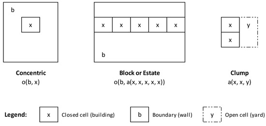
Figure 6.
Elementary generators of Portela.
The most common type in Portela is the block or estate. It is composed of five (or six, in some cases) high-rise buildings combined to form a continuous band, described here by a(x,x,x,x,x) where ‘a’ represents the relation of adjacency. Then, a boundary is superimposed to each band to form an asymmetric generator that can be declared with o(b,a(x,x,x,x,x)), where ‘o’ represents the relation of containment in coherence with the ideographic language introduced by Hillier and Hanson ([1], pp. 67–68, 78).
The concentric type is composed of a tower x inside a boundary (wall) b and can be found, namely, at the eastern border of the green park and at the northern and southern limits of the settlement (Figure 7). This is a typical asymmetric generator in the sense that the relation of x with b is different from the relation of b with x. In fact, the boundary b contains the tower x, but not the converse, a relationship that can be declared with the term o(b,x). Either block or concentric types generate depth in the sense that we need an additional step to go from the local access (‘cul-de-sac’) to the main entrance of each building in order to pass its front wall and yard.
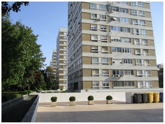
Figure 7.
Illustration of the concentric type: tower inside a wall.
Additionally, we found at the fragile south-eastern border of Portela, near the farmhouse Quinta do Cabeço and the seminary of Olivais ([26], p. 49), a careful symmetric generator with a low-rise band of two buildings attached to an open space or yard y (Figure 8), here described with a(x,x,y). We call it ‘clump’ because it is similar to the ‘beady ring’ generator from Hillier and Hanson ([1], 67–68, 78), composed of a closed cell x adjacent to an open cell y, despite its slightly different aggregation in Portela’s case.
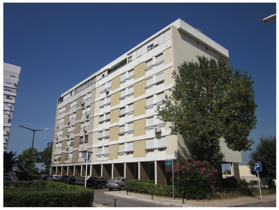
Figure 8.
Illustration of the clump type: band with an open yard.
These elementary generators were replicated alongside a ring-shaped road network. For example, the pattern found in the eastern side of the green park, alongside Rua dos Escritores (Figure 7), is a succession of adjacent towers x, each of them inside a boundary (wall) b, which can be generated with a Prolog program (https://swish.swi-prolog.org/p/egenerators.pl, accessed on 19 July 2023):
Z = o(b, x)
Z = a(o(b, x), o(b, x))
Z = a(a(o(b, x), o(b, x)), o(b, x))
Z = a(a(a(o(b, x), o(b, x)), o(b, x)), o(b, x))
…
Towers and blocks in Portela are interchangeable ([1], p. 214) in the sense that we could switch one with another without affecting the general structure of the complex too much. This is a direct consequence of the distribution of genotypes described in Figure 6. Nevertheless, we found several noninterchangeable objects at the central sector of the settlement, namely, a shopping centre with a singular tower with 20 storeys (Edifício Concórdia) and a postmodern church with a social/civic centre designed by architect Luiz Cunha [1933–2019] in 1981–1983 ([27], p. 7) and inaugurated in 1992 ([9], p. 29). These are free standing buildings surrounded by open space that maintain transpatial relations with the surrounding housing estates, that is, relations beyond those of physical adjacency ([1], p. 217). This structure can be described by the following terminals (https://swish.swi-prolog.org/p/concentric_portela.pl, accessed on 19 July 2023):
facility --> [mall].
facility --> [church].
open_space --> [equipped_garden].
housing --> [towers].
housing --> [high_rise_bands].
housing --> [low_rise_bands].
Now, we will obtain an affirmative answer from the query:
?-conc_village([mall,church,equipped_garden,towers,
high_rise_bands,low_rise_bands],[]).
in the sense that Portela can be described as a concentric village with a mall, a church and a garden at its centre and towers and high- or lower-rise bands (blocks) at its periphery. Recall from Section 3.3 that we only changed the terminals from Bororo to Portela, maintaining the syntactic rules in both cases. Thus, the two complexes have a concentric structure regulated by the same grammar.
The key syntactic measures computed with the Prolog predicates (explained in Section 3.4) for the integration core, that is, for the 25% most integrating spaces of Portela, are presented in Table 1. We obtained the same values with DepthmapX 0.8.0 except for controllability in some cases (Table 2). Relative ringiness (RR) is not provided by DepthmapX 0.8.0.

Table 1.
Syntactic measures for Portela’s integration core computed with Prolog.

Table 2.
Syntactic measures for Portela’s integration core computed with DepthmapX 0.8.0.
Typically, the most integrated spaces have high connectivity (AC), namely, the south and west sides of Avenida dos Descobrimentos (directly connected with 16 and 10 lines, respectively), Avenida da República (connected with 14 lines), Rua dos Escritores (8 lines) and Rua do Brasil (9 lines). These axes are the main road network of Portela and, alongside them, the housing estates are distributed.
However, the integration core includes less connected axes, namely, the west and east circulations around the central sector (connected with only six and three lines, respectively), Jardim Almeida Garrett (three lines), the west stairs (Escada W, three lines) and the south access to the church (Igreja S, two lines). These exceptions, among others, are highly synchronised spaces located in the middle of the settlement. Thus, Portela’s integration core includes either distributive roads or open spaces and pedestrian/local paths that are fundamental to minimise the depth effect created by ‘cul-de-sacs’ and asymmetric generators, namely, towers and blocks inside walls, as described above.
Where connectivity and integration happen together, complexes are said to be intelligible ([3], pp. 94–95). This kind of relation is not readily evident in Portela where the integration core includes secondary, pedestrian and/or less connected lines, as said. Nevertheless, Portela is an intelligible settlement in the sense that the linear correlation between connectivity and integration is high (0.74). This close relation between what can be seen from each space and what cannot be seen ([3], p. 94) is suggested by the agglomeration of points around the line in Figure 9.
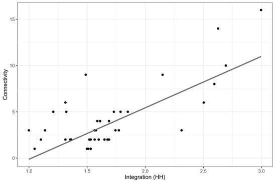
Figure 9.
Relation between connectivity and integration in Portela (intelligibility).
The two points located at the top-right of the same figure correspond to the south side of Avenida dos Descobrimentos and Avenida da República, Portela’s most connected and integrated spaces. Their prominence is also extended to relative ringiness (RR) with high values of 0.246 and 0.197, respectively (see Table 1). In fact, these two axes in conjunction with the west side of Avenida dos Descobrimentos and Rua dos Escritores form a ‘big ring’ around the central part of the complex. Besides its circulation function, this ‘ring’ structures the housing estates’ implementation. Its distributedness is also indicated by the high values of control (E) and controllability (F) associated with those axes (see Table 1). This ring is complemented in its distributive function by Rua Brasil, which has the third highest relative ringiness (0.131).
Despite its intelligibility and distributedness, Portela suffers from the ‘L-shaped problem’ associated with modern complexes ([3], pp. 147–154). This means that the probabilistic interface between two relevant categories is very poor. The malaise is illustrated by Figure 10 and consists in a highly structured nonrelation between integration and the location of retail trade and services with a very low correlation coefficient (0.14). In fact, economic activities are located in very few spaces that are not particularly integrated. This is a direct consequence of strict zoning with the concentration of economic activities in a mall with few exceptions (Rua Mouzinho de Albuquerque and Rua Luís de Camões) signalled by the outliers in the same figure. Thus, L-shaped distributions mean ruptured interfaces between qualities that should occur simultaneously in urban systems.
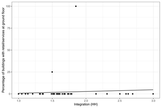
Figure 10.
Relation between incidence of retail/services on the ground floor (% of buildings) and integration in Portela (‘L-shaped problem’).
5. Discussion
The investment in a convex, open space in the middle of a complex was not original to Portela. In fact, we found the same strategy in early realisations of modern urban planning in Portugal, namely, in Nova Oeiras (1953) and Olivais Norte (1955), and in the traditional Bororo village studied by the anthropologist Claude Lévi-Strauss. However, the investment in noninterchangeable facilities, namely, a mall, a sports centre and a church highly synchronised with the surrounding buildings (towers and blocks) is a distinctive feature of this high-rise complex. The transpatial relations between housing estates and the central zone are maximised either by a distributive ringy network or by a smart grid of pedestrian paths. The result is a compact and integrated settlement with a strong identity and sense of belonging.
The potential instability of that concentric dual system, with a centre and a periphery, was minimised by forcing a clear opposition with a third element, Moscavide, a popular neighbourhood at Portela’s vicinity. As suggested by Figure 11, the structure of Portela is founded on a triskelion expressing the strict zoning between different functions (housing versus services) and also the social segregation between the inhabitants of Portela and Moscavide, originally induced by the town planner and the real estate promoter. The large circle in the figure coincides with Avenida das Descobertas, the main distributive and most integrated road of Portela, which guarantees, not only the internal circulation of the settlement, but also its connection with Moscavide, assuring some continuity between the two segregated neighbourhoods.
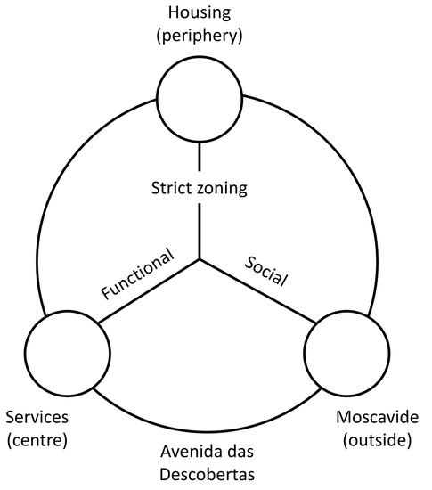
Figure 11.
Diagram of the Portela structure (triad).
We found other troubles in Portela, namely, a dissociation between the location of economic activities and integration, which is the key feature to predict human co-presence and movement in cities ([2], p. 1). The creation of depth, namely, by superimposing ‘cul-de-sacs’ and boundaries (walls) between the main streets and the housing towers and blocks is another problem found in Portela, which is minimised by the aforementioned network of pedestrian paths that favours the connection of the housing estates with the central zone.
Nevertheless, a clear structure with the replication of syntactic genotypes and the scale of the intervention (more than 10,000 inhabitants), that favours a continuous demand for the economic activities located (essentially) in the mall, might contribute for the relative success of Portela among Portuguese modern housing complexes.
6. Conclusions
The present research shows how logic programming can be used to describe the structure of a middle-sized urban settlement such as Portela as a ‘field of knowables’ or ‘intelligent system’. In fact, space syntax was founded on the premise that even complex spatial arrangements, just like natural languages, are systems governed by simple concepts and rules. Prolog was founded in the same idea in the sense that it was born as a research project to process natural languages using grammar. Thus, space syntax and logic programming are similar in reasoning and both represent knowledge in a declarative way. Indeed, the ‘problem of knowability’ is paramount not only in space syntax but also in artificial intelligence as stressed by Hillier and Hanson ([1], p. 46) in their seminal work.
In addition, the previous analyses illustrate how Prolog can be useful and attractive for students and researchers in the field of space syntax. Readily available on-line through the SWISH platform (https://swish.swi-prolog.org/, accessed on 19 July 2023), in a fancy format inspired by Jupyter notebooks (https://jupyter.org/, accessed on 19 July 2023) for Python, R or Julia, SWI-Prolog [8] can provide valuable insight in understanding the recursive nature of urban processes given some elementary generators, or in describing or even checking the structure (e.g., concentric) of a certain village. Most importantly, Prolog can compute space syntax measures such as connectivity, control, integration or even relative ringiness in a comprehensive and transparent way, using natural language and avoiding ‘black boxes’ and complex software packages.
The major drawback of using Prolog for space syntax is the time that the computation of measures such as integration can take, even using modern machines. In fact, Prolog is not an appropriate tool to analyse complex settlements or buildings. In this sense, Prolog is a readily available and flexible calculator of syntactic measures and it is particularly useful for the student or social scientist interested in small case studies such as the ones illustrated in the book The Social Logic of Space [1].
Future developments of this research will focus on the website https://www.sswprolog.net/, which centralises the links to the Prolog programmes stored in the SWISH platform [8]. The main goal is to provide a unique central point and companion for the student and/or researcher who wants to compute the metrics for a selection of buildings and settlements illustrated in the books The Social Logic of Space [1], Decoding Homes and Houses [2] and Space is the Machine [3]. Beyond Portela, the programs will cover the Barnsbury borough and the Maiden Lane Estate, both in London, the English cottages, the Ashanti palace, and the Normandy farmhouses. Eventually, a calculator of syntactic measures for Microsoft Windows will be developed using Visual Prolog.
Another rather ambitious project is the development of a natural language parser that would identify, from a simple description of an urban network (e.g., adjacency list), the elementary generators, namely, beady-ring or concentric, embodied on it. This is the kind of ‘intelligent task’ that Prolog was made for. The starting point would be the grammar described in Section 3.3.
Anyway, the inclusion of economic reasoning in space syntax theories and methods, complementing the contributions of other fields, is another line of development that will use logic or dynamic programming.
Funding
This work was supported by Fundação para a Ciência e Tecnologia (FCT), Lisbon, Portugal under a doctorate auxiliary researcher grant with the reference CUBE-PhD-CEEC/1 from Católica Lisbon Research Unit in Business & Economics (UID/GES/00407/2020).
Institutional Review Board Statement
Not applicable.
Informed Consent Statement
Not applicable.
Data Availability Statement
Data and code available on SWISH (https://swish.swi-prolog.org/, accessed on 19 July 2023) with the links provided in this article and centralised in the Space Syntax with Prolog website (https://www.sswprolog.net/, accessed on 19 July 2023).
Conflicts of Interest
The author declares no conflict of interest.
Abbreviations
The following abbreviations are used in this manuscript:
| AC | Axial Connectivity |
| CAD | Computer-Aided Design |
| D | Depth |
| DV | Diamond Value |
| E | Control |
| F | Controllability |
| FCT | Portuguese Foundation for Science and Technology |
| GIS | Geographic Information System |
| HH | Hillier and Hanson |
| I | Integration |
| IHH | Integration, Hillier and Hanson definition |
| MD | Mean Depth |
| N | Nodes |
| N.C. | Rue Nungesser et Coli, Paris, France |
| RA | Relative Asymmetry |
| RRA | Real Relative Asymmetry |
| RR | Relative Ringiness |
| SWISH | SWI-Prolog for SHaring |
| TD | Total Depth |
| UCL | University College of London |
References
- Hillier, B.; Hanson, J. The Social Logic of Space; Cambridge University Press: Cambridge, UK, 1984. [Google Scholar]
- Hanson, J. Decoding Homes and Houses; Cambridge University Press: Cambridge, UK, 1998. [Google Scholar]
- Hillier, B. Space Is the Machine: A Configurational Theory of Architecture; Space Syntax: London, UK, 2007. [Google Scholar]
- Heitor, T.; Pinelo Silva, J. A Sintaxe Espacial e o Ambiente Construído—Análise Morfológica. In O Estudo da Forma Urbana em Portugal; Oliveira, V., Marat-Mendes, T., Pinho, P., Eds.; Universidade do Porto: Porto, Portugal, 2015; pp. 147–189. [Google Scholar]
- Turner, A. Depthmap 4—A Researcher’s Handbook; Bartlett School of Graduate Studies, University College of London: London, UK, 2004. [Google Scholar]
- Colmerauer, A.; Roussel, P. The birth of Prolog. ACM SIGPLAN Not. 1993, 28, 37–52. [Google Scholar] [CrossRef]
- Kowalski, R.A. The early years of Logic Programming. Commun. Assoc. Comput. Mach. 1988, 31, 38–43. [Google Scholar] [CrossRef]
- Wielemaker, J.; Schrijvers, T.; Triska, M.; Lager, T. SWI-Prolog. Theory Pract. Log. Program. 2012, 12, 67–96. [Google Scholar] [CrossRef]
- Ferreira, B.M. Urbanização da Portela. In Optimistic Suburbia? The Students’ Perspective 2; Milheiro, A.V., Ed.; FCT/ISCTE-IUL: Lisboa, Portugal, 2016; pp. 9–29. [Google Scholar]
- Pereira, S.M. Mass housing in Lisbon: Sometimes it works. J. Hous. Build. Environ. 2017, 32, 513–532. [Google Scholar] [CrossRef]
- Salgado, M.; Lourenço, N. Atlas Urbanístico de Lisboa; Argumentum: Lisboa, Portugal, 2006. [Google Scholar]
- Pereira, S.M.; Corte-Real, M. Modern estates and the production of Lisbon’s suburbs: From the planned to the lived neighbourhood. City Territ. Archit. 2022, 9, 13. [Google Scholar] [CrossRef]
- Land, C.; Hücking, K.J.; Trigueiros, L. Architecture in Lisbon and the South of Portugal since 1974; Editorial Blau: Lisboa, Portugal, 2005. [Google Scholar]
- Makowsky, J.A. Why Horn Formulas Matter in Computer Science: Initial Structures and Generic Examples. J. Comput. Syst. Sci. 1987, 34, 266–292. [Google Scholar] [CrossRef]
- Blackburn, P.; Bos, J.; Striegnitz, K. Learn Prolog Now! Texts in Computing; College Publications: London, UK, 2006. [Google Scholar]
- Flach, P. Simply Logical: Intelligent Reasoning by Example; John Wiley and Sons: Hoboken, NJ, USA, 1994. [Google Scholar]
- Monteys, X. Le Corbusier: Obras y Proyectos/Obras e Projectos; Editorial Gustavo Gili: Barcelona, Spain, 2005. [Google Scholar]
- Hillier, B.; Jones, L.; Penn, A.; Jianming, X.; Grajewski, T. The Architecture of the Maiden Lane Estate: A Second Opinion; Unit for Architectural Studies, Bartlett School of Architecture and Planning, University College of London: London, UK, 1989. [Google Scholar]
- Sbriglio, J. Immeuble 24 N.C. et Appartment Le Corbusier; Fondation Le Corbusier/Birkhäuser: Paris, France; Basel, Switzerland, 1996. [Google Scholar]
- Troubetzkoy, N.S. Principles de Phonologie; Librairie C. Klincksieck: Paris, France, 1949. [Google Scholar]
- Lévi-Strauss, C. Structural Anthropology; Basic Books: New York, NY, USA, 1963. [Google Scholar]
- Malinowski, B. The Sexual Life of Savages in North-Western Melanesia; Readers League of America and Eugenics Publishing Company: New York, NY, USA, 1929. [Google Scholar]
- Fernandes, P.A. Introduction of non-topological costs in syntactic analyses: The case of Gulbenkian estate. In Proceedings of the Back to Human Scale International Meeting, Lisbon, Portugal, 24–25 November 2022; pp. 3.1–3.8. [Google Scholar]
- Teklenburg, J.A.F.; Timmermans, H.J.P.; van Wagenberg, A.F. Space Syntax: Standardised Integration Measures and Some Simulations. Environ. Plan. B Urban Anal. City Sci. 1993, 20, 347–357. [Google Scholar] [CrossRef]
- Krüger, M.; Vieira, A.P. Scaling relative asymmetry in space syntax analysis. J. Space Syntax. 2012, 3, 194–203. [Google Scholar]
- de Stoop, A. Quintas e Palácios nos Arredores de Lisboa; Livraria Civilização: Porto, Portugal, 1999. [Google Scholar]
- Rocha, J.; Ferreira, J.; Cunha, L. Igreja Paroquial de Cristo-Rei da Portela; Paróquia de Cristo-Rei da Portela: Portela, Portugal, 2000. [Google Scholar]
Disclaimer/Publisher’s Note: The statements, opinions and data contained in all publications are solely those of the individual author(s) and contributor(s) and not of MDPI and/or the editor(s). MDPI and/or the editor(s) disclaim responsibility for any injury to people or property resulting from any ideas, methods, instructions or products referred to in the content. |
© 2023 by the author. Licensee MDPI, Basel, Switzerland. This article is an open access article distributed under the terms and conditions of the Creative Commons Attribution (CC BY) license (https://creativecommons.org/licenses/by/4.0/).