
Urban Planning of Coastal Adaptation under Sea-Level Rise: An Agent-Based Model in the VIABLE Framework


Abstract
:1. Introduction
2. Materials and Methods
2.1. Agent-Based Modelling
2.2. The VIABLE Framework
2.3. The Single-Agent Urban Coastal Model
2.4. Mathematical Formulation of the Model
2.4.1. Agent Dynamics
2.4.2. Agent Investments (Optimizing Behavior)
2.4.3. State Dynamics
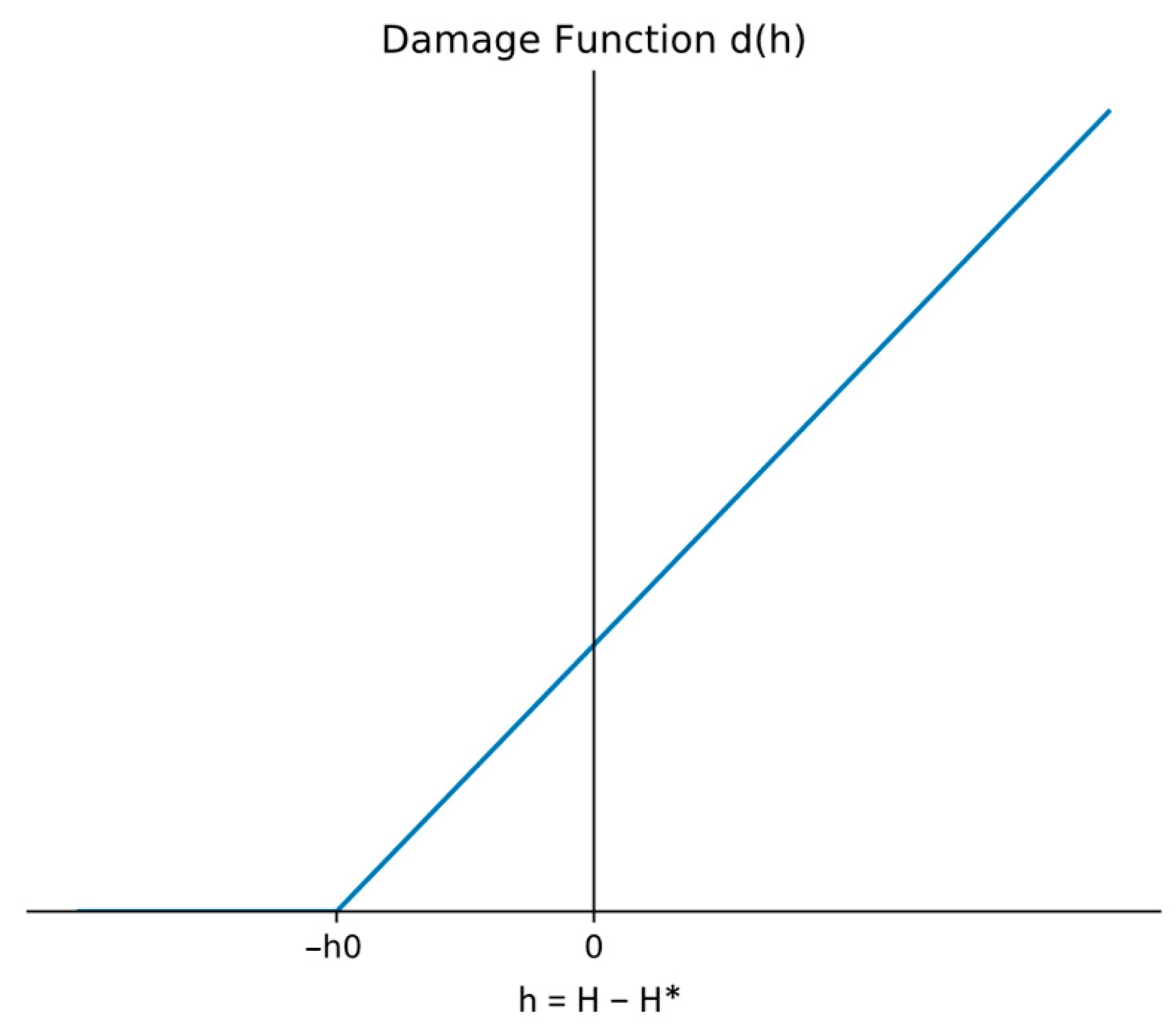
2.4.4. Extreme Sea-Level Events
2.4.5. Agent Action
2.4.6. Investment Efficiency
2.4.7. Units and Values of Model Parameters
3. Results
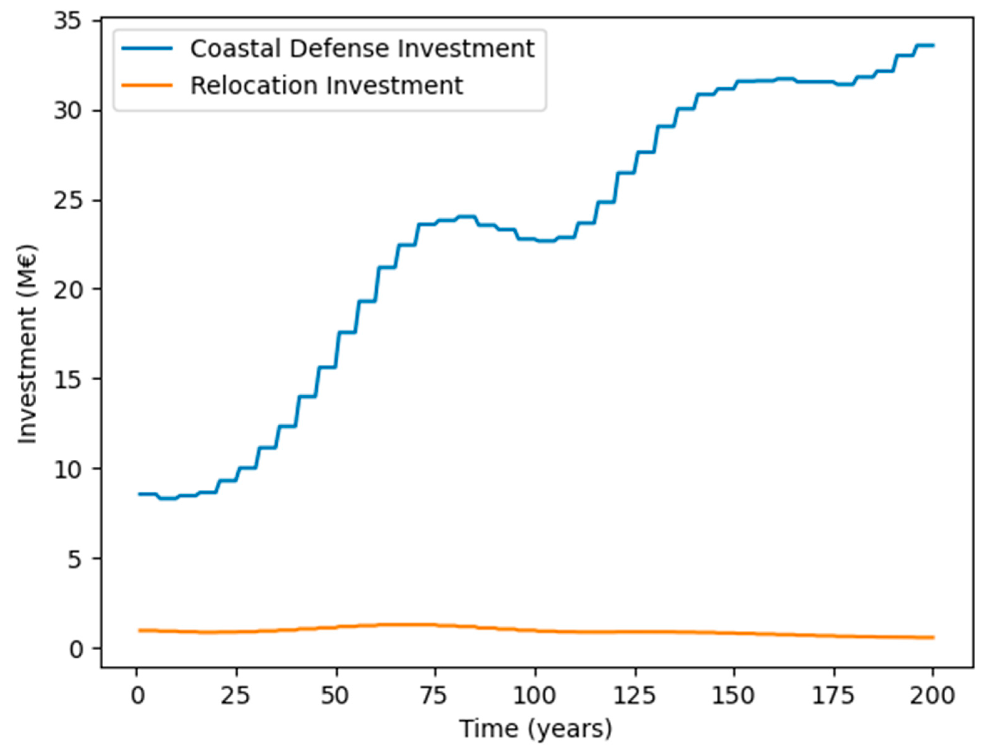
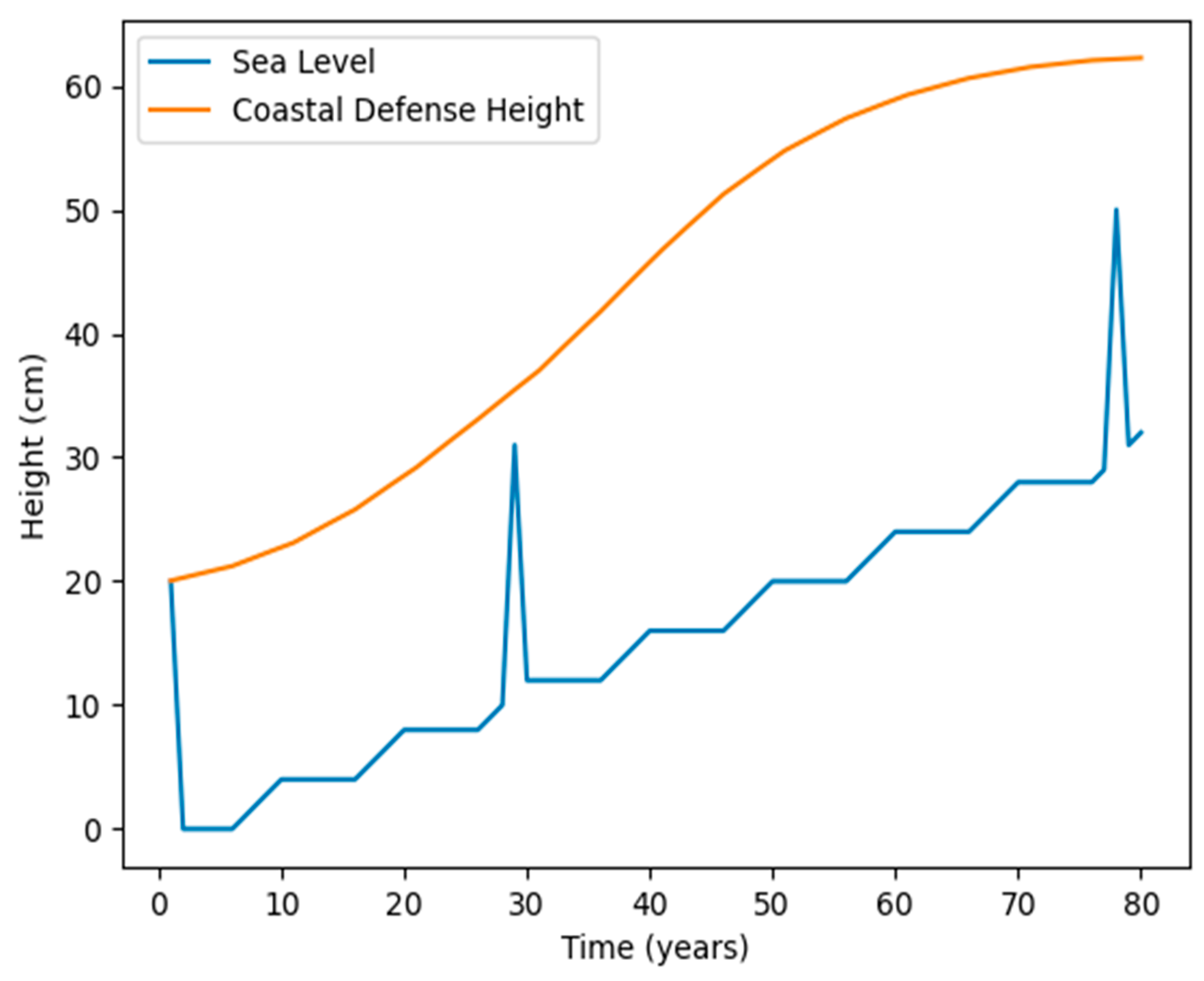
3.1. Agent Response
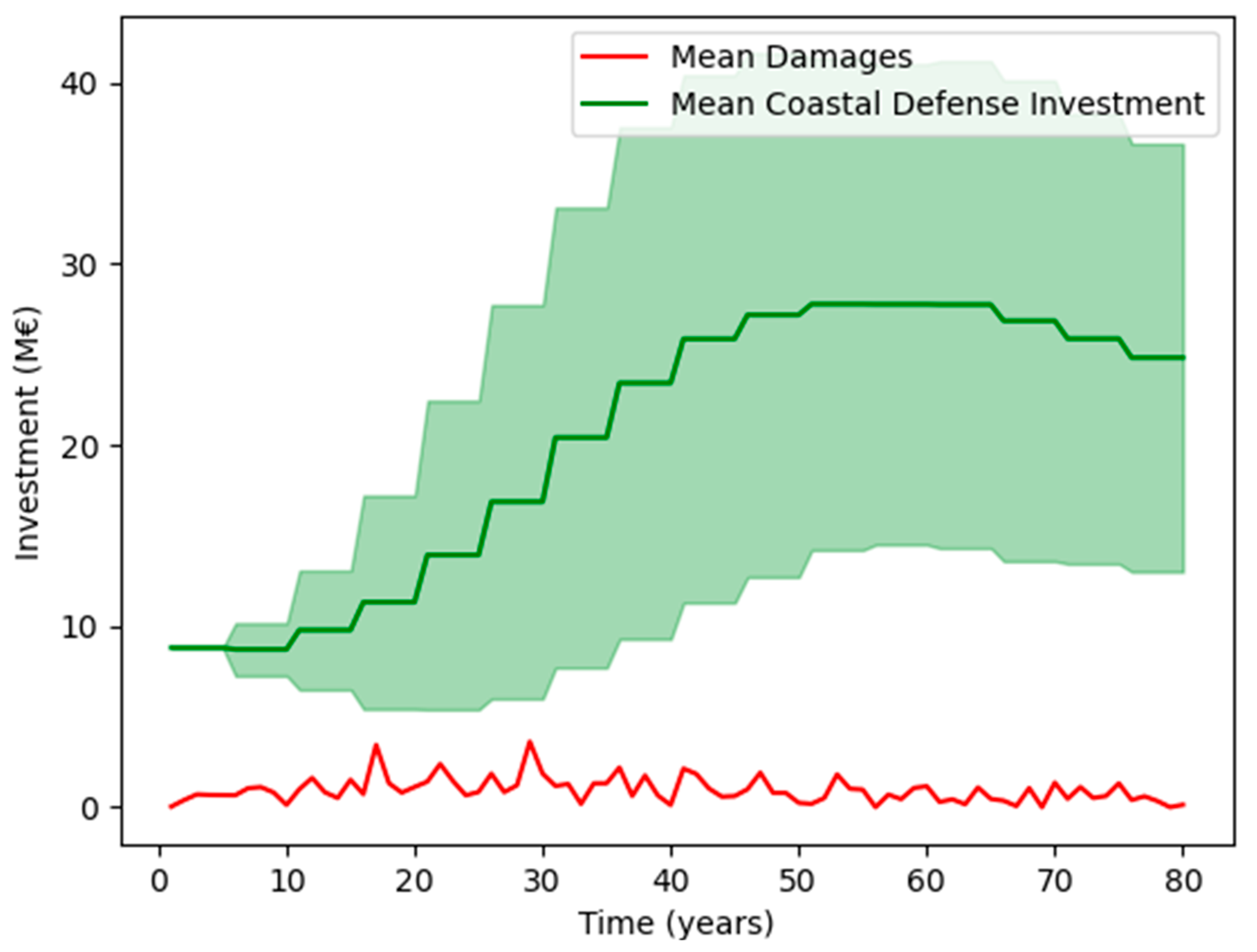
3.2. Effect of Timing of Extreme Events
3.3. Adaptation Success
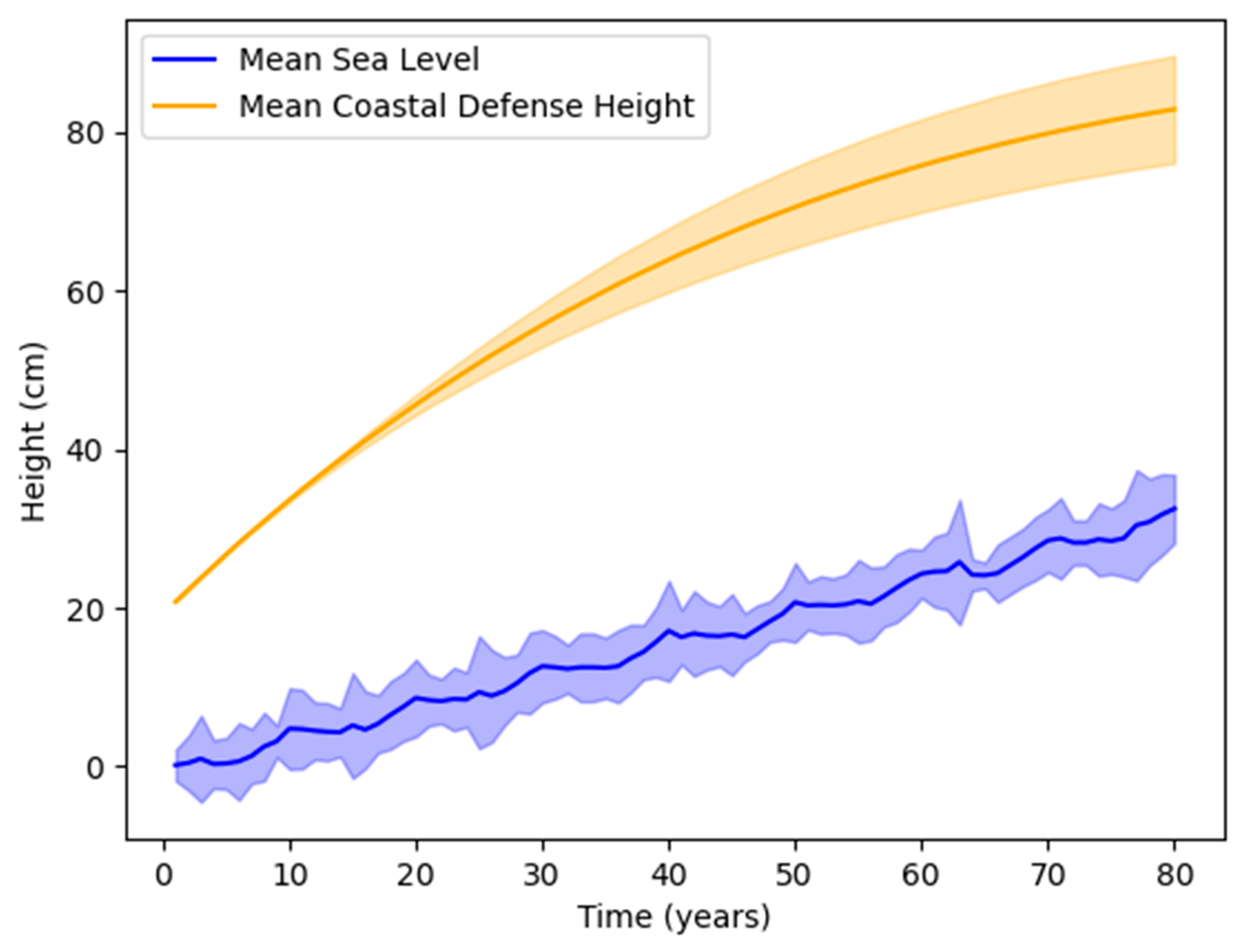
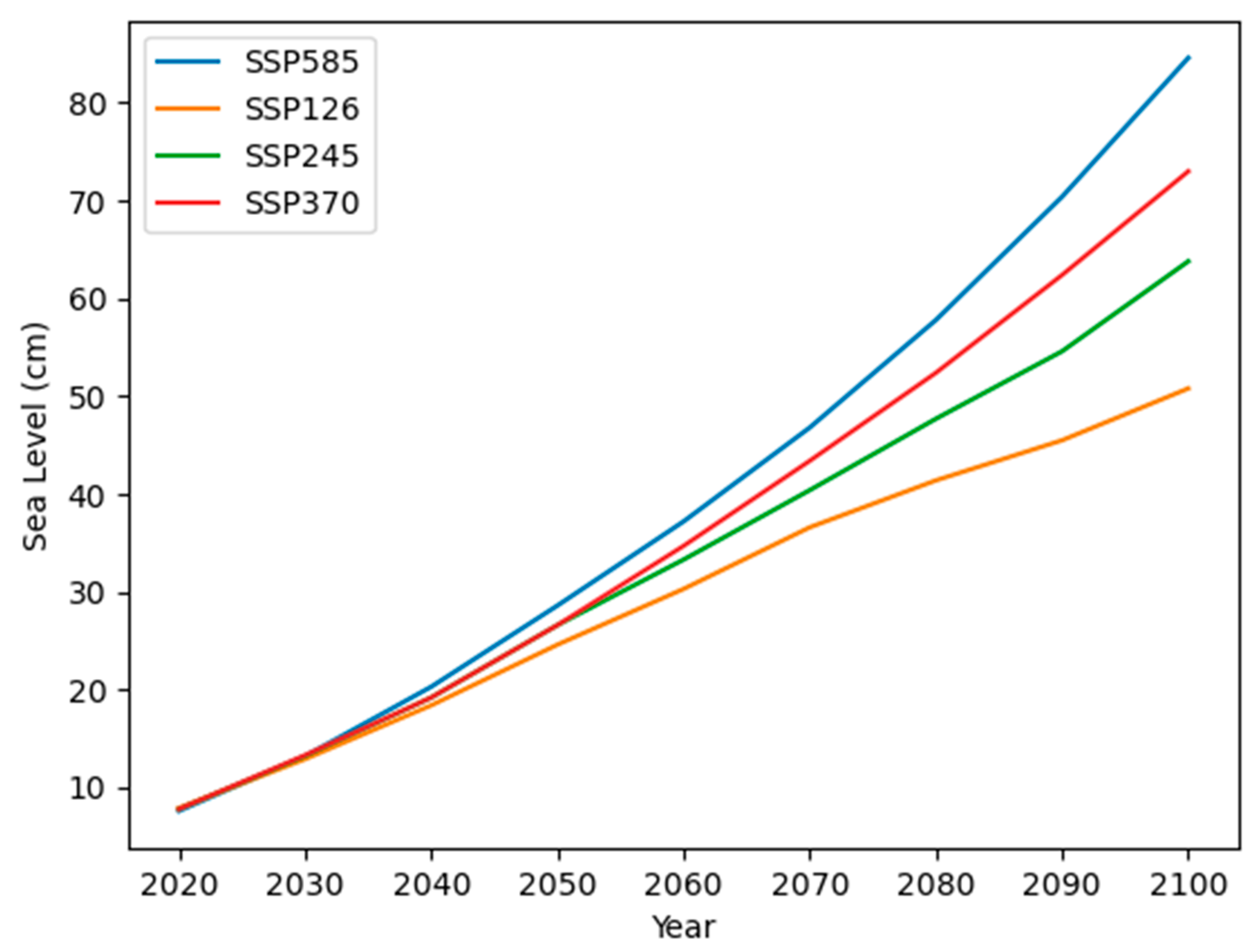
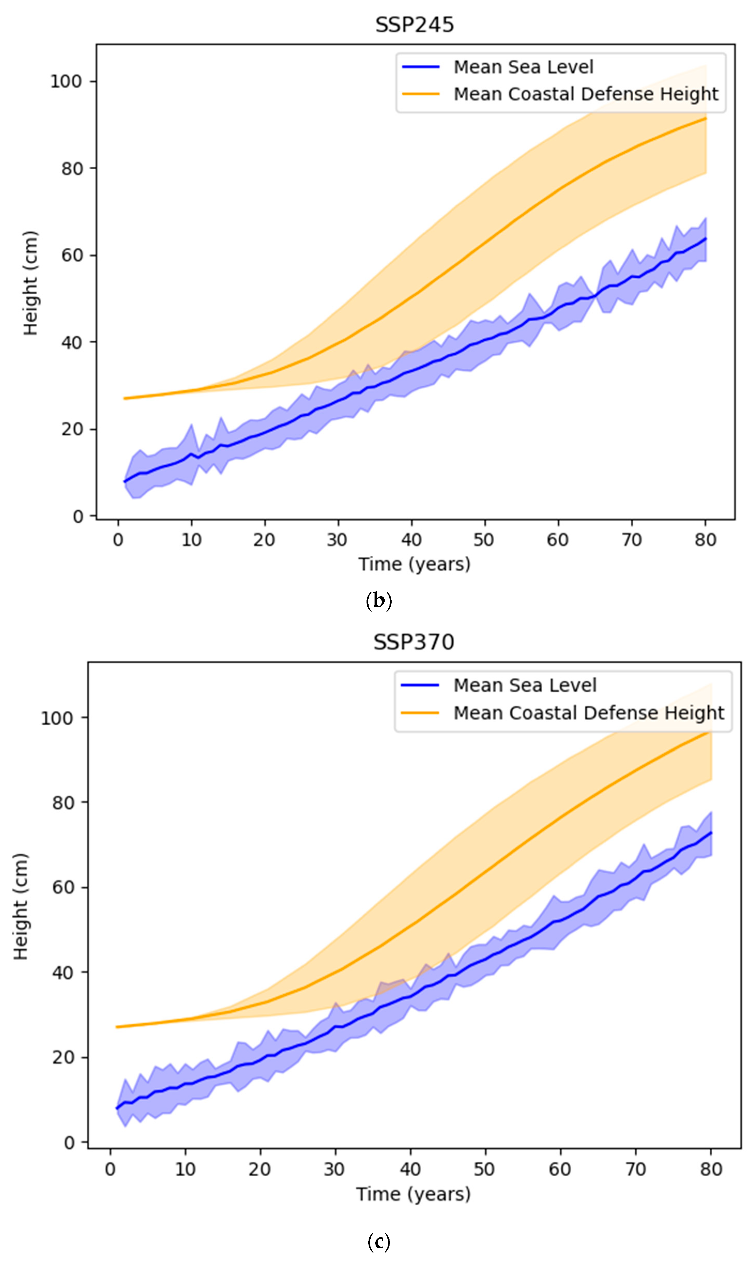
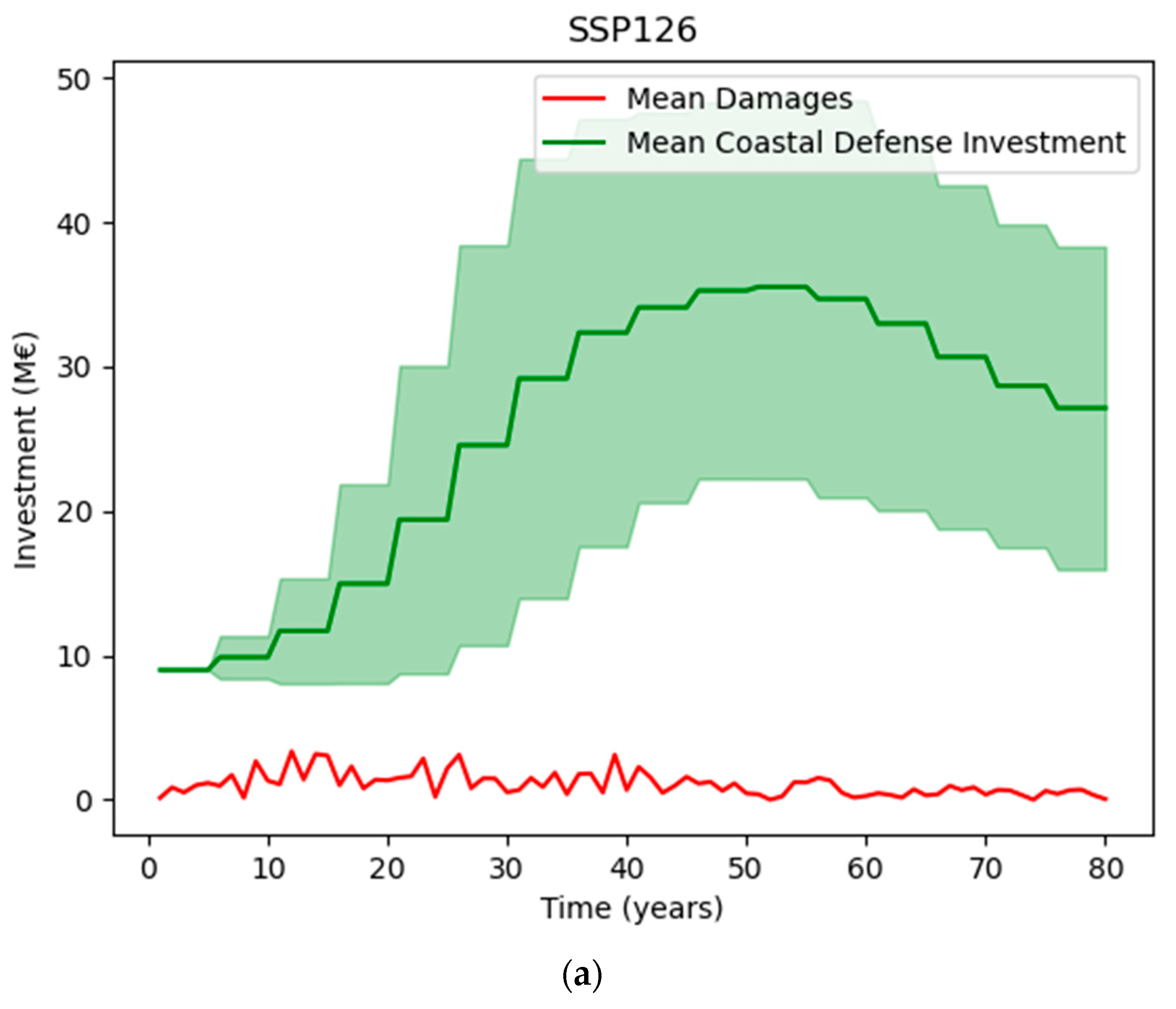
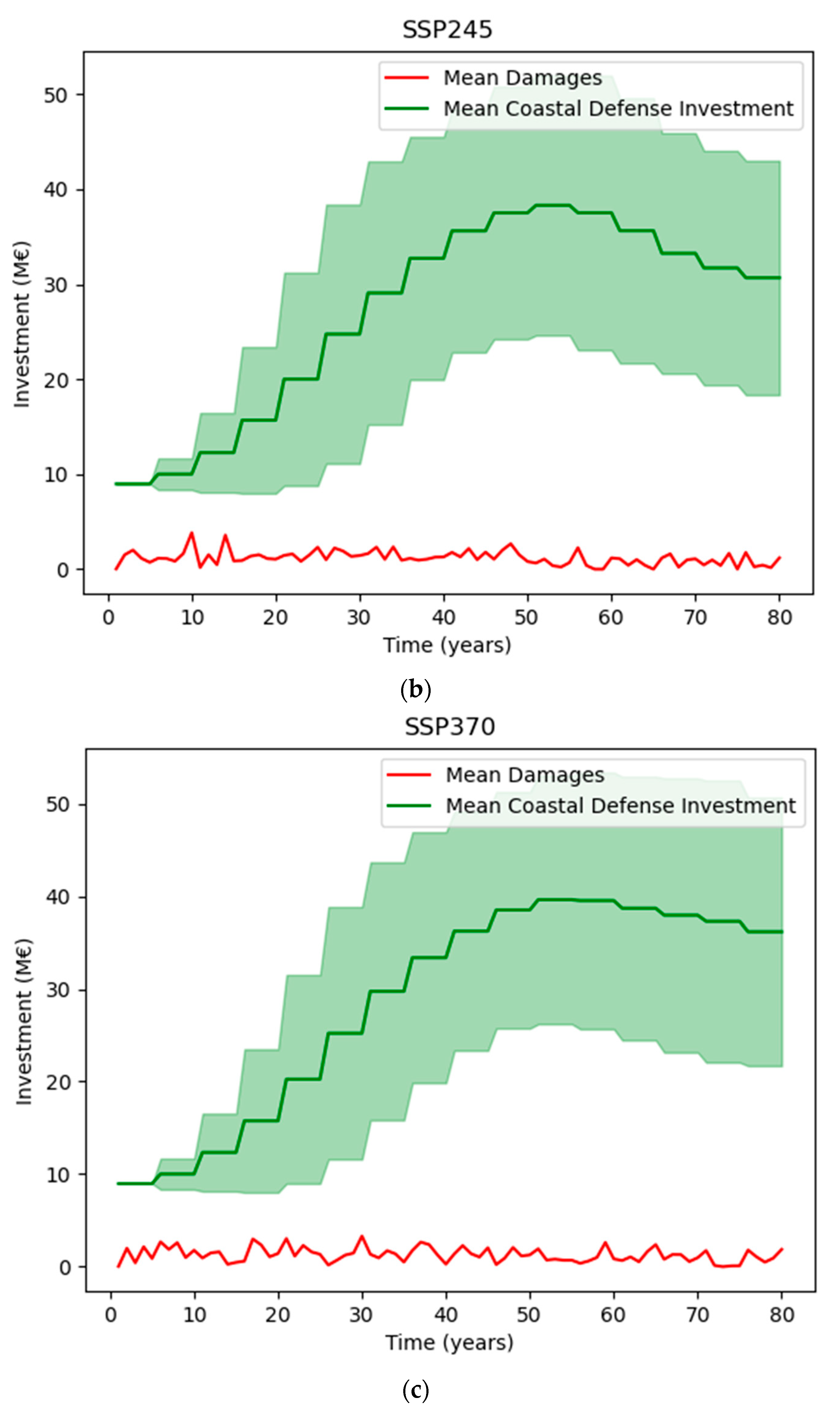
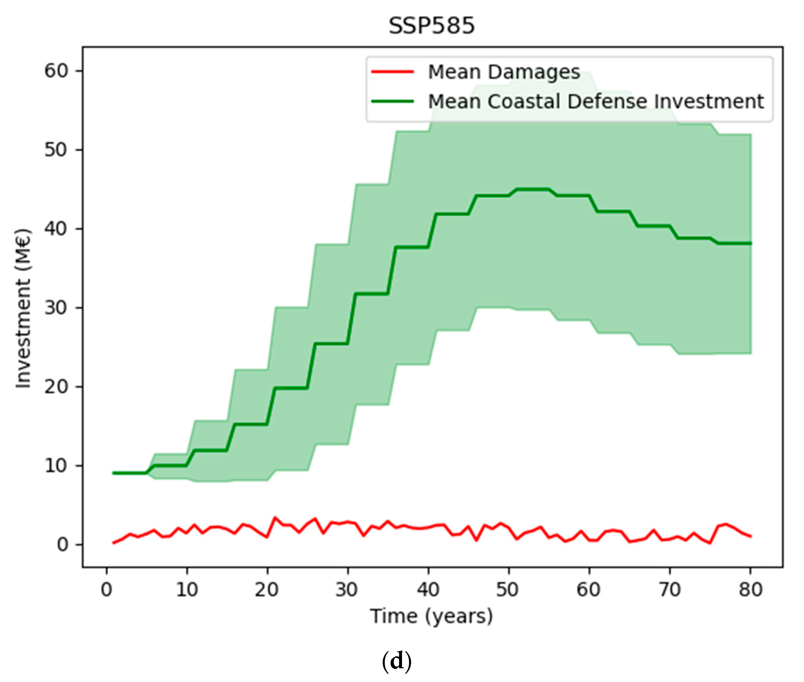
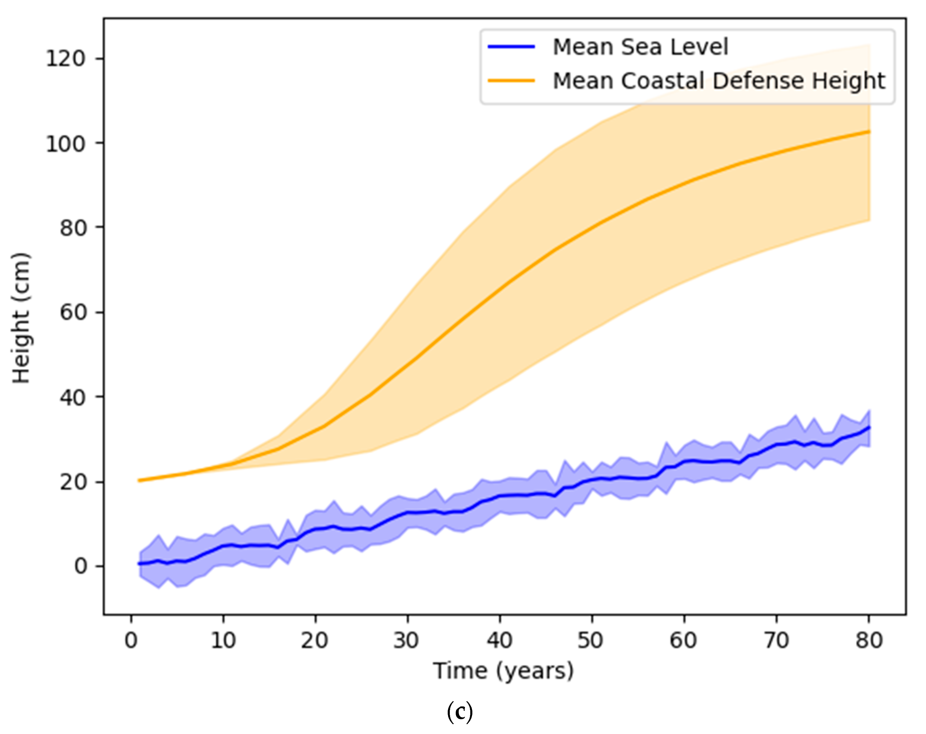
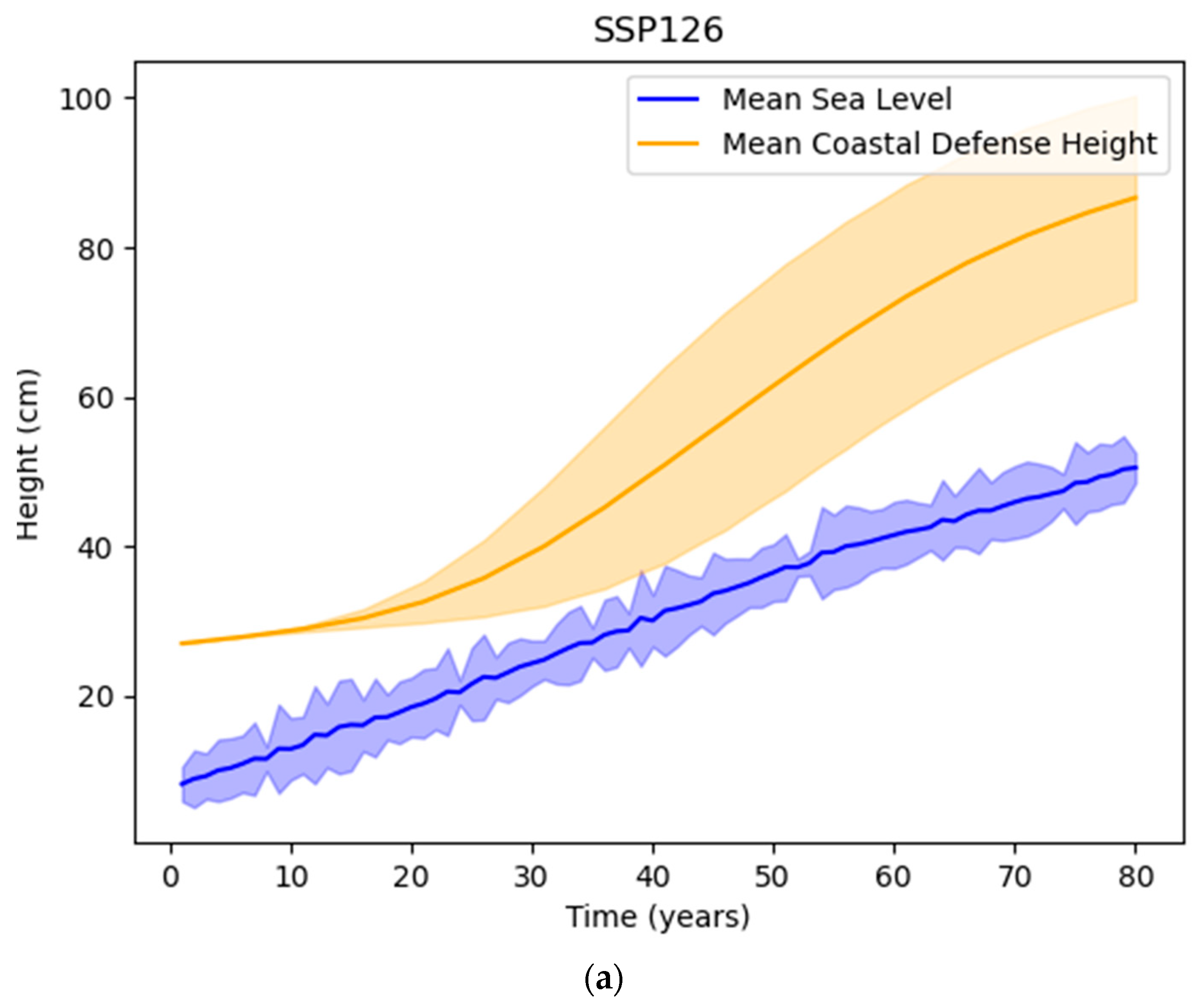
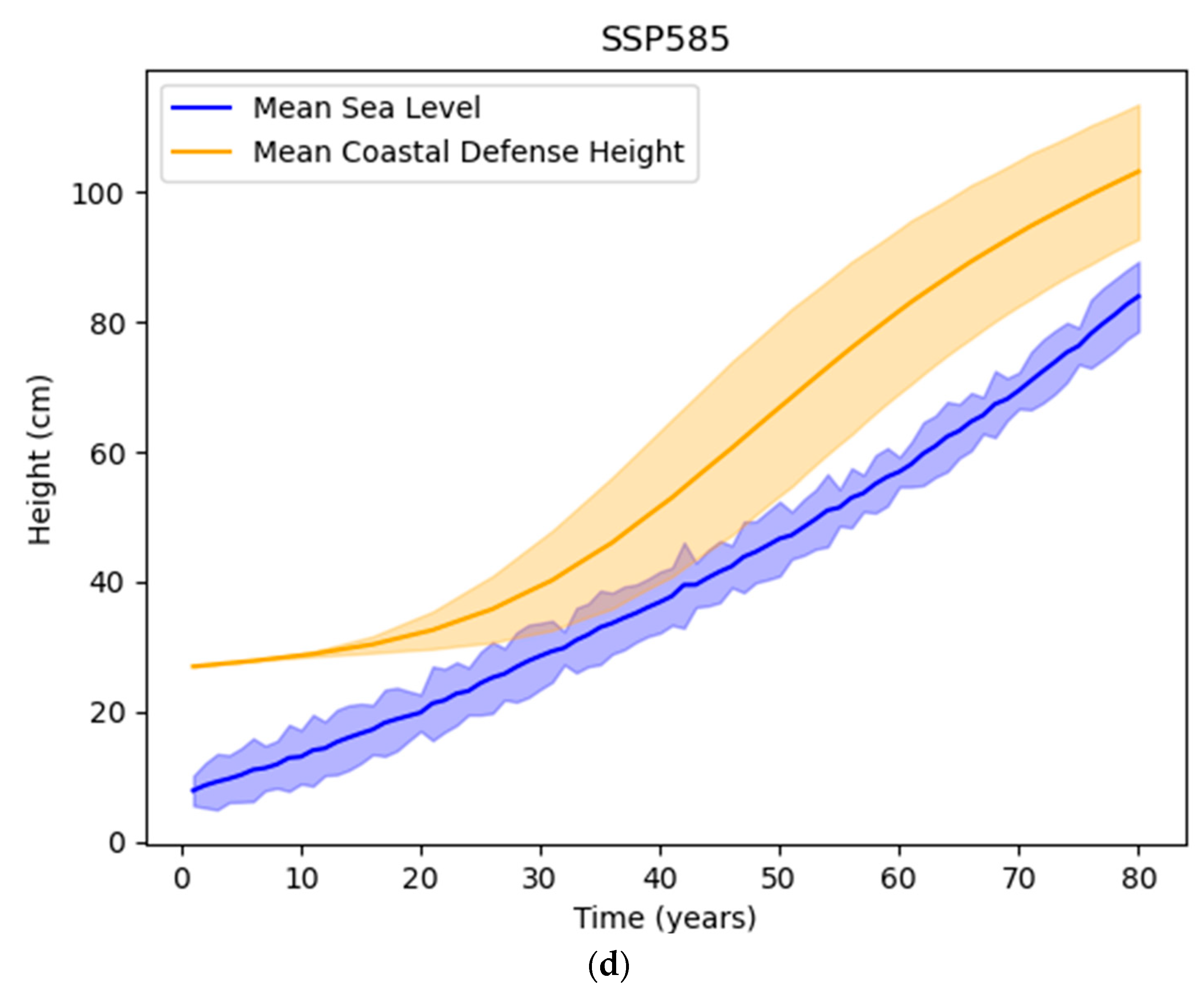
3.4. Scenarios of Sea-Level Rise
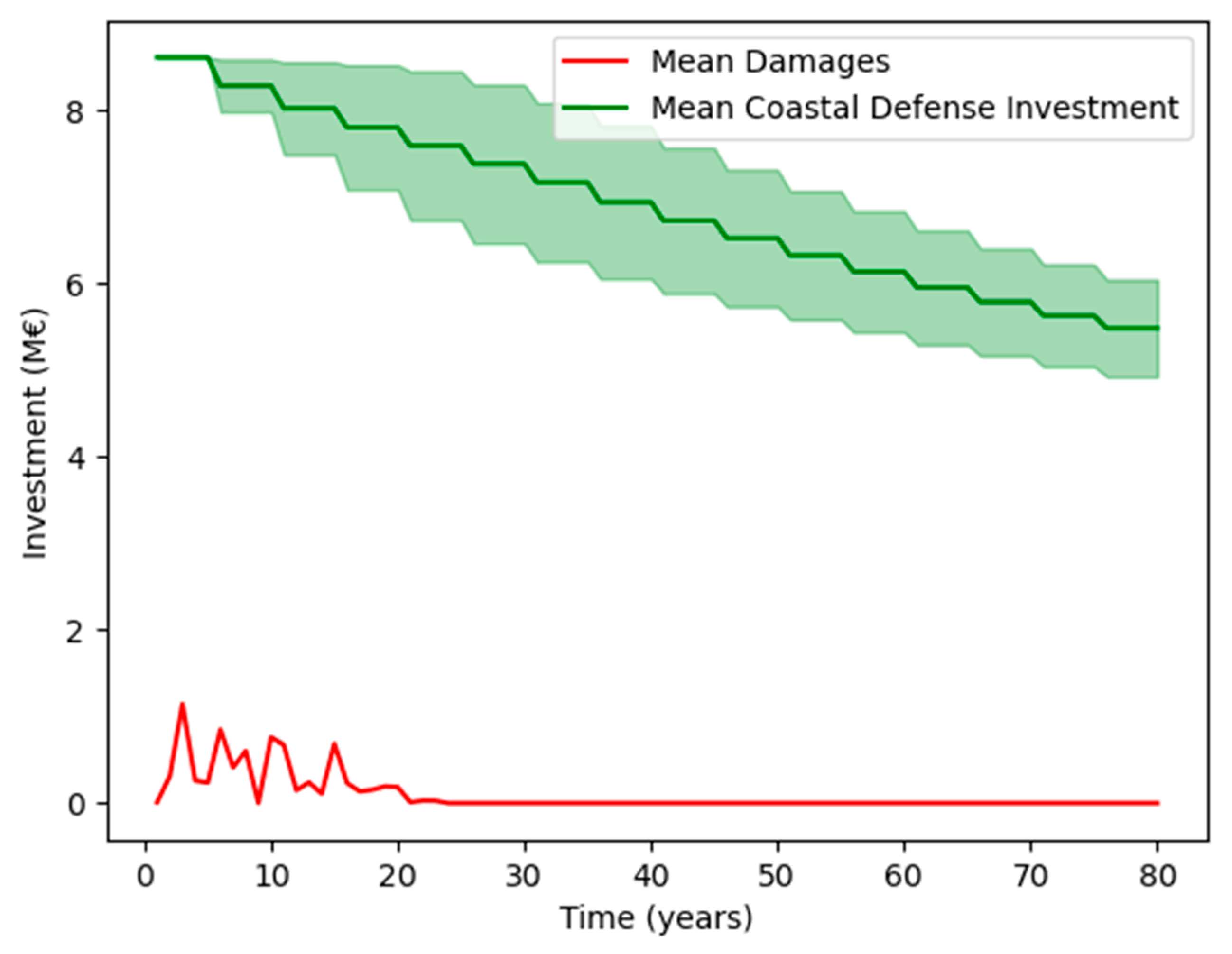
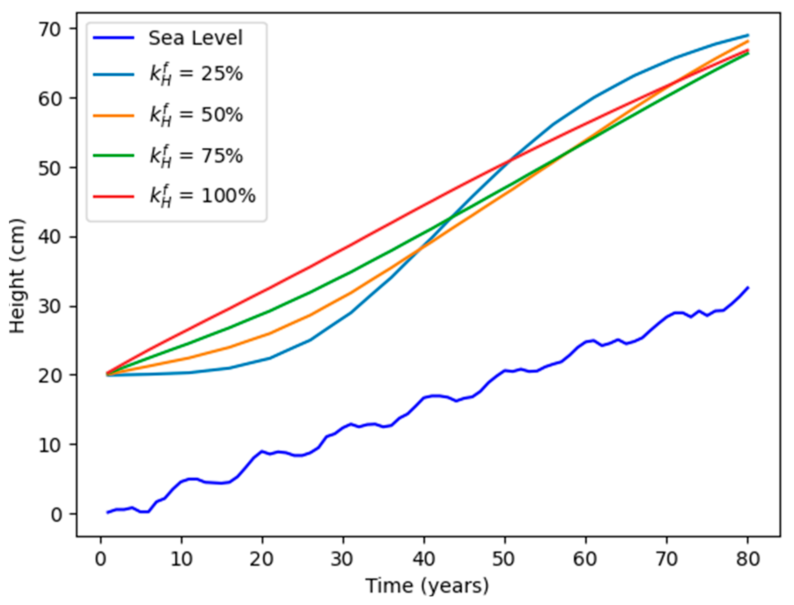
3.5. Effect of “Hedging”
4. Discussion
5. Conclusions
Author Contributions
Funding
Data Availability Statement
Acknowledgments
Conflicts of Interest
Appendix A

Appendix B

- Since either or holds true, we first make these substitutions:
- We then compute , and , where:
- We conduct a similar substitution for the case, where :
- We now similarly compute , and , where:
- The values of and that correspond to the maximum value of out of the terms computed in Steps 2 and 4, are the target values and .
Appendix B.1. Special Case for α and β
References
- UNPD (United Nations, Department of Economic and Social Affairs, Population Division), World Urbanization Prospects: The 2018 Revision. The United Nations: New York. 2019. Available online: https://www.google.com/url?sa=t&rct=j&q=&esrc=s&source=web&cd=&ved=2ahUKEwjbhNCD9K2AAxVEyGEKHYD1A8YQFnoECBYQAQ&url=https%3A%2F%2Fpopulation.un.org%2Fwup%2Fpublications%2FFiles%2FWUP2018-Report.pdf&usg=AOvVaw33RksR7fLXlpPYrI7Q4Poq&opi=89978449 (accessed on 1 July 2023).
- Fox-Kemper, B.; Hewitt, H.T.; Xiao, C.; Aðalgeirsdóttir, G.; Drijfhout, S.S.; Edwards, T.L.; Golledge, N.R.; Hemer, M.; Kopp, R.E.; Krinner, G.; et al. Ocean, Cryosphere and Sea Level Change. In Climate Change 2021: The Physical Science Basis. Contribution of Working Group I to the Sixth Assessment Report of the Intergovernmental Panel on Climate Change; Masson-Delmotte, V., Zhai, P., Pirani, A., Connors, S.L., Péan, C., Berger, S., Caud, N., Chen, Y., Goldfarb, L., Gomis, M.I., et al., Eds.; Cambridge University Press: Cambridge, UK; New York, NY, USA,, 2021; pp. 1211–1362. [Google Scholar]
- Pörtner, H.-O.; Roberts, D.C.; Adams, H.; Adelekan, I.; Adler, C.; Adrian, R.; Aldunce, P.; Ali, E.; Begum, R.A.; Friedl, B.B.; et al. Climate Change 2022: Impacts, Adaptation and Vulnerability; Cambridge University Press: Cambridge, UK; New York, NY, USA,, 2022; pp. 37–118. [Google Scholar]
- Schelling, T.C. Dynamic models of segregation. J. Math. Sociol. 1971, 1, 143–186. [Google Scholar]
- Sakoda, J.M. The checkerboard model of social interaction. J. Math. Sociol. 1971, 1, 119–132. [Google Scholar]
- Yang, L.E.; Scheffran, J.; Süsser, D.; Dawson, R.; Chen, Y.D. Assessment of flood losses with household responses: Agent-based simulation in an urban catchment area. Environ. Model. Assess. 2018, 23, 369–388. [Google Scholar]
- Dawson, R.J.; Peppe, R.; Wang, M. An agent-based model for risk-based flood incident management. Nat. Hazards 2011, 59, 167–189. [Google Scholar]
- Taberna, A.; Filatova, T.; Roy, D.; Noll, B. Tracing resilience, social dynamics and behavioral change: A review of agent-based flood risk models. Socio-Environ. Syst. Model. 2020, 2, 17938. [Google Scholar]
- BenDor, T.K.; Scheffran, J. Agent-Based Modeling of Environmental Conflict and Cooperation; Taylor & Francis Group: Boca Raton, FL, USA, 2018; p. 333. [Google Scholar]
- Yang, L.E.; Hoffmann, P.; Scheffran, J.; Rühe, S.; Fischereit, J.; Gasser, I. An agent-based modeling framework for simulating human exposure to environmental stresses in urban areas. Urban Sci. 2018, 2, 36. [Google Scholar]
- Kind, J.M. Economically efficient flood protection standards for the Netherlands. J. Flood Risk Manag. 2014, 7, 103–117. [Google Scholar] [CrossRef]
- Vrijling, J.K.; van Hengel, W.; Houben, R.J. Acceptable risk as a basis for design. Reliab. Eng. Syst. Saf. 1998, 59, 141–150. [Google Scholar] [CrossRef]
- Jonkman, S.N.; Hillen, M.M.; Nicholls, R.J.; Kanning, W.; van Ledden, M. Costs of adapting coastal defences to sea-level rise—New estimates and their implications. J. Coast. Res. 2013, 29, 1212–1226. [Google Scholar]
- Kron, W.; Müller, O. Efficiency of flood protection measures: Selected examples. Water Policy 2019, 21, 449–467. [Google Scholar]
- Garner, G.; Hermans, T.H.J.; Kopp, R.; Slangen, A.; Edwards, T.; Levermann, A.; Nowicki, S.; Palmer, M.; Smith, C.J.; Fox-Kemper, B.; et al. IPCC AR6 WGI Sea Level Projections. Version 20210809. PO.DAAC, CA, USA. Available online: https://podaac.jpl.nasa.gov/announcements/2021-08-09-Sea-level-projections-from-the-IPCC-6th-Assessment-Report (accessed on 13 May 2022).
- Kopp, R.E.; Garner, G.G.; Hermans, T.H.J.; Jha, S.; Kumar, P.; Slangen, A.B.A.; Turilli, M.; Edwards, T.L.; Gregory, J.M.; Koubbe, G.; et al. The Framework for Assessing Changes To Sea-level (FACTS) v1.0-rc: A platform for characterizing parametric and structural uncertainty in future global, relative, and extreme sea-level change, EGUsphere [preprint]. Available online: https://podaac.jpl.nasa.gov/announcements/2021-08-09-Sea-level-projections-from-the-IPCC-6th-Assessment-Report (accessed on 13 May 2022).
- Jevrejeva, S.; Jackson, L.P.; Riva, R.E.M.; Grinsted, A.; Moore, J.C. Coastal sea level rise with warming above 2 °C Proc. Natl. Acad. Sci. USA 2016, 113, 13342–13347. [Google Scholar] [CrossRef] [PubMed]


| Scenario Name | Scenario Description (Changes in Sea Level H in cm) |
|---|---|
| Gradual (deterministic) | H + 1 for five steps after every five timesteps |
| Gradual with extreme events (probabilistic) | H + 1 + x for five steps after every five timesteps, where x is a randomized value that has an increasing chance to be non-zero with time |
| Model Units and Their Equivalents | |
| Timestep (time units) | Years |
| Height Units (for sea-level rise and coastal defense height) | Centimeters |
| Monetary Units | Millions euro (M €) |
| Area Units | Square kilometers |
| Model Parameters | |
| Adaptation rate α | 0.5 |
| Fractional investment efficiency into coastal defense development kHf | 0.5 |
| Investment efficiency into city relocation kRf | 0.1 |
| Defense depreciation rate | 0.05 cm/yr |
| Baseline percentage probability of extreme sea-level events at each timestep | 3.00 |
| Increase in percentage probability of extreme sea-level events per timestep | 0.01 |
| Initial Variable Values | |
| Coastal Area | 10 sq. km |
| Inland Area | 10 sq. km |
| Unit Income from the coastal territory | 20 M €/sq. km |
| Scenario | ACD | ADA (%) | ACB (%) |
|---|---|---|---|
| High-cost | 1.00 | 97.07 | 69.78 |
| Low-cost | 1.00 | 97.12 | 201.63 |
| Scenario | ACD | ADA (%) | ACB (%) |
|---|---|---|---|
| SSP126 | 1.00 | 97.06 | 55.81 |
| SSP245 | 1.00 | 97.05 | 52.81 |
| SSP370 | 1.00 | 97.05 | 49.86 |
| SSP585 | 1.00 | 97.03 | 46.45 |
| Scenario | ACD | ADA (%) | ACB (%) |
|---|---|---|---|
| = 2 | 1.00 | 97.12 | 20.15 |
| = 1 | 1.00 | 97.12 | 32.87 |
| = 0.5 | 1.00 | 97.11 | 42.95 |
Disclaimer/Publisher’s Note: The statements, opinions and data contained in all publications are solely those of the individual author(s) and contributor(s) and not of MDPI and/or the editor(s). MDPI and/or the editor(s) disclaim responsibility for any injury to people or property resulting from any ideas, methods, instructions or products referred to in the content. |
© 2023 by the authors. Licensee MDPI, Basel, Switzerland. This article is an open access article distributed under the terms and conditions of the Creative Commons Attribution (CC BY) license (https://creativecommons.org/licenses/by/4.0/).
Share and Cite
Sengupta, S.; Kovalevsky, D.V.; Bouwer, L.M.; Scheffran, J. Urban Planning of Coastal Adaptation under Sea-Level Rise: An Agent-Based Model in the VIABLE Framework. Urban Sci. 2023, 7, 79. https://doi.org/10.3390/urbansci7030079
Sengupta S, Kovalevsky DV, Bouwer LM, Scheffran J. Urban Planning of Coastal Adaptation under Sea-Level Rise: An Agent-Based Model in the VIABLE Framework. Urban Science. 2023; 7(3):79. https://doi.org/10.3390/urbansci7030079
Chicago/Turabian StyleSengupta, Shubhankar, Dmitry V. Kovalevsky, Laurens M. Bouwer, and Jürgen Scheffran. 2023. "Urban Planning of Coastal Adaptation under Sea-Level Rise: An Agent-Based Model in the VIABLE Framework" Urban Science 7, no. 3: 79. https://doi.org/10.3390/urbansci7030079
APA StyleSengupta, S., Kovalevsky, D. V., Bouwer, L. M., & Scheffran, J. (2023). Urban Planning of Coastal Adaptation under Sea-Level Rise: An Agent-Based Model in the VIABLE Framework. Urban Science, 7(3), 79. https://doi.org/10.3390/urbansci7030079