Article

Interaction between Development Intensity: An Evaluation of Alternative Spatial Weight Matrices

1
School of Automobile, Chang’an University, Xi’an 710064, China
2
College of Transportation Engineering, Chang’an University, Xi’an 710064, China
3
School of Civil Engineering, The University of Sydney, Sydney 2006, Australia
*
Author to whom correspondence should be addressed.
Urban Sci. 2023, 7(1), 22; https://doi.org/10.3390/urbansci7010022
Submission received: 2 December 2022 / Revised: 5 February 2023 / Accepted: 6 February 2023 / Published: 9 February 2023

Abstract

:
This paper investigates the spatial dependency of job and worker densities for the Minneapolis–St. Paul (Twin Cities) metropolitan area using census block level data from 2002 to 2017. A spatial weight matrix is proposed, considering the statistical expression of data, referred to as the correlation matrix, which detects the variations of dependencies among spatial units in both direction and level. The superior performance of the correlation matrix is demonstrated through a series of spatial regression models to predict land use patterns, in comparison with the conventionally used adjacency matrix as well as the accessibility matrix.

1. Introduction

To ensure the continuing adequacy of public services and infrastructure, it is important to have accurate estimates of short-term changes related to the population and employment [1,2,3,4,5]. Although considerable efforts have been made [6,7,8,9], forecasts remain unsatisfying. Historically, there has been a shortage of detailed data used for land use pattern analysis due to the limited data collection and storage. It is especially difficult to capture spatial interdependence between land uses because various factors affect land use at different spatial scales with distinct temporal dynamics and interact with each other in an intricate way [10,11,12].
Agent-based models or cell-based models have emerged within the past two decades as increasingly attractive alternatives with which to estimate land use [13]. Grounded in the systems and complexity theory, they represent a system from the bottom up, that is, they account for an agent’s behavior in space and/or time, along with interactions among agents [14]. Specifically, they predict future land use patterns from the initial states of land use agents and the effects of neighboring land use agents by using transition rules. Although diverse methods have been employed to describe the transition rules [3,4], these rules typically extract information from immediate cells, ignoring more dispersed interactions.
Regression models can clearly explain the land use system and relate land use patterns with their previous states and a variety of exogenous variables including location characteristics [15], neighborhood effects [15,16], the effects of transport [17], and other socioeconomic factors [18]. The levels of neighborhood effects in these models are usually assumed to decline with distance based on Tobler’s first law of geography [19]; however, directions, do not change, that is, the effects are always negative or positive. Given that competitive and complementary relationships in space have been witnessed at the same time [20,21,22], we considered whether job and worker densities compete and collaborate at the same time to address the several questions specified below:
Is there spatial dependency between job density and worker density?
Does the spatial dependency of job and worker densities change in direction and level?
How can the spatial interaction of job and worker densities be captured?
How helpful is information about changes elsewhere in predicting density here?
Because spatial weight matrices are used to express the changes of dependencies between spatial units (places) in spatial regression models [23,24,25], we proposed a new spatial weight matrix, named the correlation matrix, that can capture the variation of spatial dependency in direction and strength and then compared it with two kinds of basic spatial weight matrixes, i.e., an adjacency matrix and accessibility matrix, to corroborate if it shows advantages when explaining the land use changes.
This paper is structured as follows: Section 2 discusses three spatial weight matrices, including the adjacency, accessibility, and correlation matrices, that are able to capture changes in spatial dependency. The land use spatial regression model and estimation method are specified in Section 3. Section 4 presents all data resources, and the fitting results are provided in Section 5. Section 6 applies the model to predict the land use intensity for the Twin Cities in 2022. Section 7 concludes the paper.

2. Spatial Weight Matrix

Figure 1 summarizes the design idea of this research. As illustrated, we discuss three spatial weight matrices, including the adjacency, accessibility, and correlation matrices, and compare their performances in land use density regression models using indices, e.g., R2 and mean absolute percentage error, based on the Twin Cities metropolitan area census block data. The land use spatial model with a correlation matrix is further applied to predict density in 2022 for the Twin Cities.
The spatial weight matrix is firstly discussed here, as it is the key element of a spatial regression model. Data collections, model specifications, and applications can be found in the following sections.
Based on Tobler’s first law of geography [19], spatial analyzers widely assume that levels of dependencies among spatial units decline with distance and propose boundary based and distance-based spatial weight matrices. Later, an accessibility matrix is proposed to develop a transport network that can eliminate the disutility of the distance [26]. However, the two matrices only include non-negative elements and cannot capture a change in the direction of the spatial dependency. To compensate for the shortage, we propose the construction of a correlation coefficient-based spatial weight matrix that has both positive and negative elements. In this section, we explore three spatial weight matrices and compare them in detail.

2.1. Adjacency Matrix

Several basic formats of boundary based and distance-based spatial weight matrices have been provided by Anselin (1988) [27]; here, we introduce the most basic one, called the adjacency matrix. The adjacency matrix only considers the interaction of adjacent places, with an implicit assumption that a nearby place is more likely to have an effect than one that is far away, as human activities are constrained by distance [19].
The adjacency matrix is an n * n matrix, in which an element is 1 if two places presented by the corresponding row and column are geographically adjacent; otherwise, it is 0. The diagonal elements are recorded as 0 (spatial units are not adjacent to themselves).

2.2. Accessibility Matrix

The concept of accessibility is examined in two ways in land use models. On the one hand, accessibility is generally considered as the distance of a spatial unit from the road network in land use cover models [28,29,30]. On the other hand, in models exploring land use and transport interactions, it is typically explained as opportunities of a place to access various facilities, such as employment or shopping [26]. We aimed to model land use intensity, considering the effect of the transport network. Therefore, the latter was adopted here.
Conventionally, accessibility considers not only the changes of transport networks that alter place-to-place travel times, but also the change of land use that alters the distribution of opportunities, such as jobs or workers [31,32,33]. Because land use intensity data have already expressed the opportunity features, the accessibility matrix here relies only on the place-to-place travel time to represent the change in the spatial dependency level in land use models. Specifically, as shown in Equation (1), it is constructed as an n * n matrix, in which an element is equal to 1 if the place, presented by the corresponding row, can access another that is presented by the corresponding column by using the defined travel mode within a predetermined travel time threshold; otherwise, it equals 0. The diagonal elements are again set to 0.
W a ( i , j ) = 0 i f   C i , j T 1 i f   C i , j > T
where:
W a ( i , j ) : accessibility between place i and j ;
C i , j : travel time between place i and j ;
T : travel time threshold.

2.3. Correlation Matrix

Beyond geography and transport networks, there are other many factors that cause job and worker densities at different spatial places to be correlated, including economic factors, cultural networks, and policies [15]. The data reflect the effects of all these factors, therefore the correlation reflected by it might disclose spatial dependency between densities after temporal detrending. Hence, a correlation matrix is proposed.
The correlation matrix is an n * n matrix in which each element shows the Pearson correlation coefficient between two places, which are represented by the corresponding row and column; the inputs are two vectors of observations, such as job or worker densities in every given year. Note that the temporal trend in the data must be eliminated. To do so, the value of each spatial unit is normalized based on the regional value. Specifically, the job density at each place is divided by the total number of jobs in the study area. The same normalization process applies to the worker density.
Because the data are values rather than ordinals [34,35], the Pearson correlation coefficient is chosen. However, the problem is that it cannot be calculated when values of one or both vectors are constant. When this situation occurs, we adhere to the following:
(1) set the Pearson correlation coefficient as 1 if the densities of both places remain the same over the years (they are perfectly correlated);
(2) set the Pearson correlation coefficient as 0 if the density of the one place remains unchanged, yet the other varies over the years (they are not correlated).
A positive value in the correlation matrix indicates that two spatial units are complementary to each other, while a negative value indicates that they are competitive. We believe that such a statistical expression of the data shows advantages over the adjacency and accessibility matrices, as it can capture a complex spatial relationship, including one that is complementary and competitive, at the same time [36].

2.4. An Illustration of Three Spatial Weight Matrices

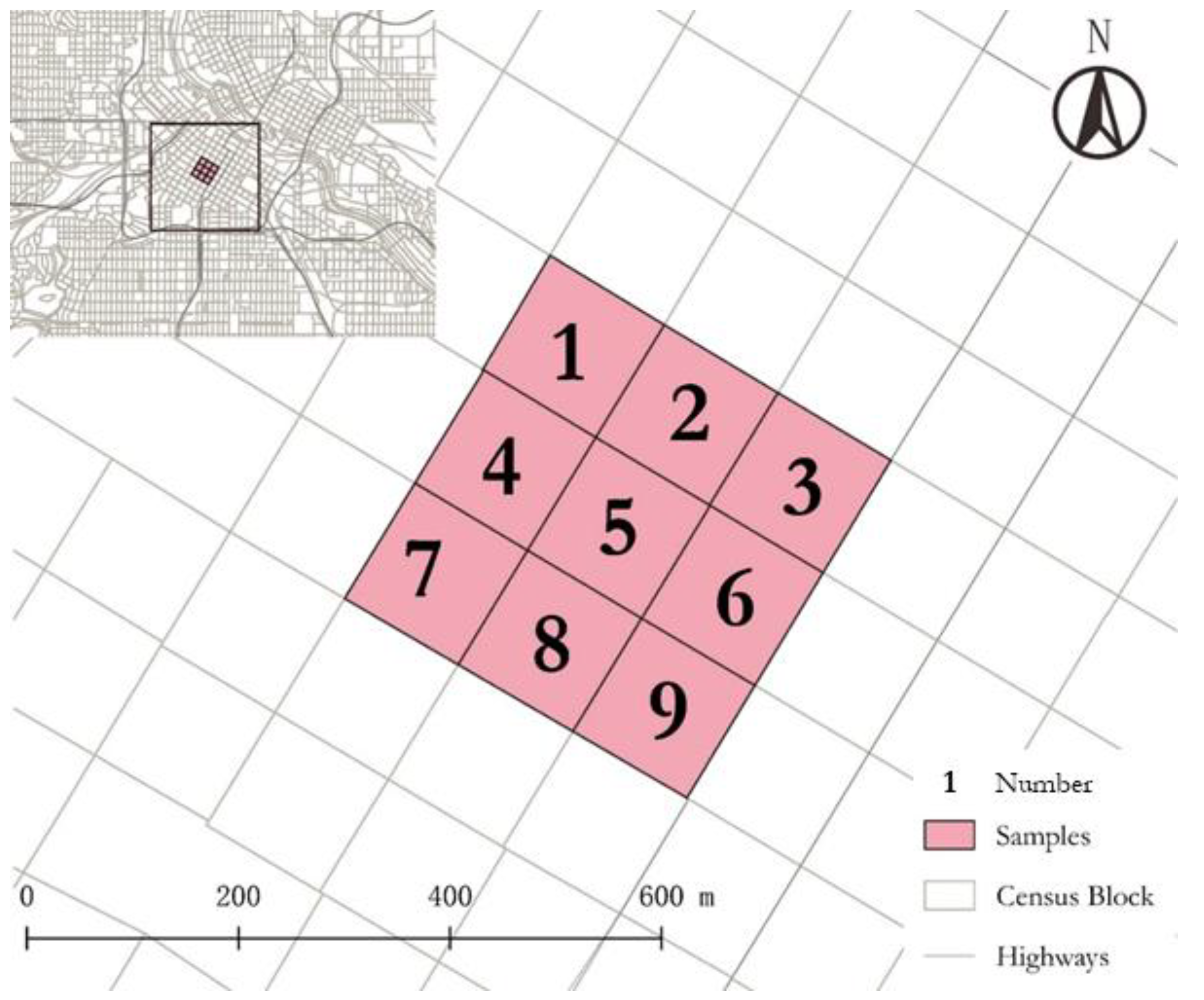
To illustrate, we extracted nine census blocks from downtown Minneapolis (see Figure 2) to further explain how to build the spatial weight matrices. Its adjacency matrix, accessibility matrix (by walking within 10 min), and correlation matrix are displayed in Equations (2)–(4), respectively.
W n = 1 2 3 4 5 6 7 8 9 1 2 3 4 5 6 7 8 9 0 1 0 1 1 0 0 0 0 1 0 1 1 1 1 0 0 0 0 1 0 0 1 1 0 0 0 1 1 0 0 1 0 1 1 0 1 1 1 1 0 1 1 1 1 0 1 1 0 1 0 0 1 1 0 0 0 1 1 0 0 1 0 0 0 0 1 1 1 1 0 1 0 0 0 0 1 1 0 1 0
W a = 1 2 3 4 5 6 7 8 9 1 2 3 4 5 6 7 8 9 0 1 1 1 1 1 0 1 1 1 0 1 1 1 1 0 1 1 1 1 0 1 1 1 0 1 1 1 1 1 0 1 1 0 1 1 1 1 1 1 0 1 0 1 1 1 1 1 1 1 0 0 1 1 0 0 0 0 0 0 0 0 0 1 1 1 1 1 1 0 0 1 1 1 1 1 1 1 0 1 0
W c = 1 2 3 4 5 6 7 8 9 1 2 3 4 5 6 7 8 9 0.13 0.00 0.27 0.26 −0.46 −0.43 0.48 0.42 −0.12 −0.23 −0.39 0.34 0.54 −0.51 0.17 0.28 −0.10 −0.17 0.72 −0.31 0.49 0.33 −0.34 −0.30 0.51 0.05 −0.18 −0.66 0.46 −0.77 −0.73 0.65 0.51 −0.73 0.08 0.26 −0.82 0.24 −0.41 −0.34 0.17 0.32 −0.39 −0.21 −0.13 −0.38 0.66 −0.49 −0.53 0.73 0.21 −0.54 −0.34 −0.29 0.21 0.22 −0.30 −0.27 −0.41 −0.02 −0.20 0.03 0.54 −0.48 0.70 −0.75 −0.74 0.88 0.35 −0.08 −0.33 0.51 −0.76 0.58 −0.37 −0.39 0.46 0.42 −0.48 −0.27 −0.16
From Equation (2), we can observe that the adjacency matrix is symmetric. Its elements consist of 0 and 1, where 1 denotes that two blocks are geographically connected, while 0 represents the opposite scenario. When used as a weight, the value reflects whether or not two blocks have a spatial dependency. However, both levels and directions of dependencies are treated the same for all adjacent blocks.
Similarly, the accessibility matrix shown in Equation (3) comprises 0 and 1, demonstrating that it also determined the levels and directions of spatial dependencies to be the same. However, it uses a different dependency judgement condition so that two nonadjacent places can be spatially dependent, such as, for example, block 1 and block 7. This is caused by traffic networks that eliminate disutility caused by distance. Note that the accessibility matrix in this example is symmetric; however, in real-world cases, it can be asymmetric when considering the directionalities of traffic networks.
Unlike the adjacency and accessibility matrices, there are negative values in the correlation matrix shown in Equation (4), which reveals a change in the direction of the dependencies between spatial units; that is, the complementary or competitive relationships change. The matrix is asymmetric, and, more importantly, it has closely distinguished values, demonstrating that the correlation matrix can reflect the specific dependent strength between any two places.
According to the differences among those three spatial weight matrices, we postulate that the correlation matrix can most effectively capture the spatial dependency when it is applied to model land use intensity; the accessibility matrix second most effective, while the adjacency matrix is the least effective.

3. Model Specification and Statistical Technique

To validate the proposed correlation matrix, we applied spatial regression models, including the correlation matrix and the other two spatial matrices mentioned above, to fit land use intensity data. These spatial regression models and the respective estimator of their parameters are discussed as follows.

3.1. Model Specification

The models were specified to predict job density and worker density, respectively.
Assuming that all else is equal, we would expect the density in each place to follow the system trend: when the economy blooms, the total number of jobs increases, regional density increases, and job density everywhere increases on average; when it withers, they all decrease. Similarly, worker density in each place also has a positive relationship with the total number of workers. As shown in Equation (5), to control the system trend, we used a normalized density (job/worker density at a spatial unit over the total number of jobs/workers in the study area), herein referred to as density, instead of the density value itself as the dependent variable.
D U , i , t = ρ U , i , t N U , t
where:
D U , i , t : normalized density, specifically, job ( D e , i , t ) or worker ( D w , i , t ), at place i in year t ;
ρ U , i , t : density at place i in year t ;
N U , t : average density of jobs or workers in the study area in year t .
As the built environment changes slowly, we expect that the density (job and worker) at one time can be largely explained by the density in the previous time period [17]. Thus, we applied a lagged independent variable to the regression model.
The spatial variables of both job and worker densities are incorporated in each model as they are expected to mutually affect each other in space. The spatial variables are specifically calculated as the spatial weight matrices defined in Section 2, multiplying by vectors consisting of the state changes of each place that is lagged in order to disentangle the causes and effects of the spatial influences between the job and worker densities.
Accordingly, the general model for the density is expressed as,
ln D U , i , t = θ 0 + θ 1 ln D U , i , t - k + θ 2 W M ln D e , i , t - k D e , i , t - 2 k + θ 3 W M ln D w , i , t - k D w , i , t - 2 k
where:
k : lag length;
W M : spatial weight matrix. Specifically, M can be adjacency ( n ), accessibility ( a ) or correlation ( c ).

3.2. Statistical Technique

The feasible generalized least-squares (FGLS) estimator, panel-corrected standard error (PCSE) estimator, and non-parametric covariance matrix estimator are widely used to regress cross-sectional time-series (panel) data because they adjust the standard errors of the estimated parameters for time and spatial dependencies in the residuals and can ensure the validity of the statistical results [37,38]. The FGLS estimator has a poor performance for panel data when the number of time periods is less than the number of places (observation locations). The PCSE estimator requires an assumption of the spatial dependency correction’s form [38]. The non-parametric time-series covariance matrix estimator, proposed by Driscoll and Kraay (1998) [39], applies a Newey–West-type correction to the sequence of the cross-sectional averages of the moment conditions and is consistent independent of the cross-sectional dimension [24,25]. For the sake of generality, we selected the nonparametric time-series covariance matrix estimator to fit the land use intensity models. This was performed using the Stata software program, specifically through the xtscc command.

4. Data

This section introduces the data sources used to fit the land use regression models.
The longitudinal employer–household dynamic (LEHD) Origin–Destination Employment Statistics (LODESs) dataset, released by the U.S. Census Bureau (2017) [40], provides state-based census block level employment statistics from 2002 to 2017, in which the Workplace Area Characteristic (WAC) table reports the number of employees in each census block; moreover, the Residence Area Characteristic (RAC) table shows the number of workers living in each residential block.
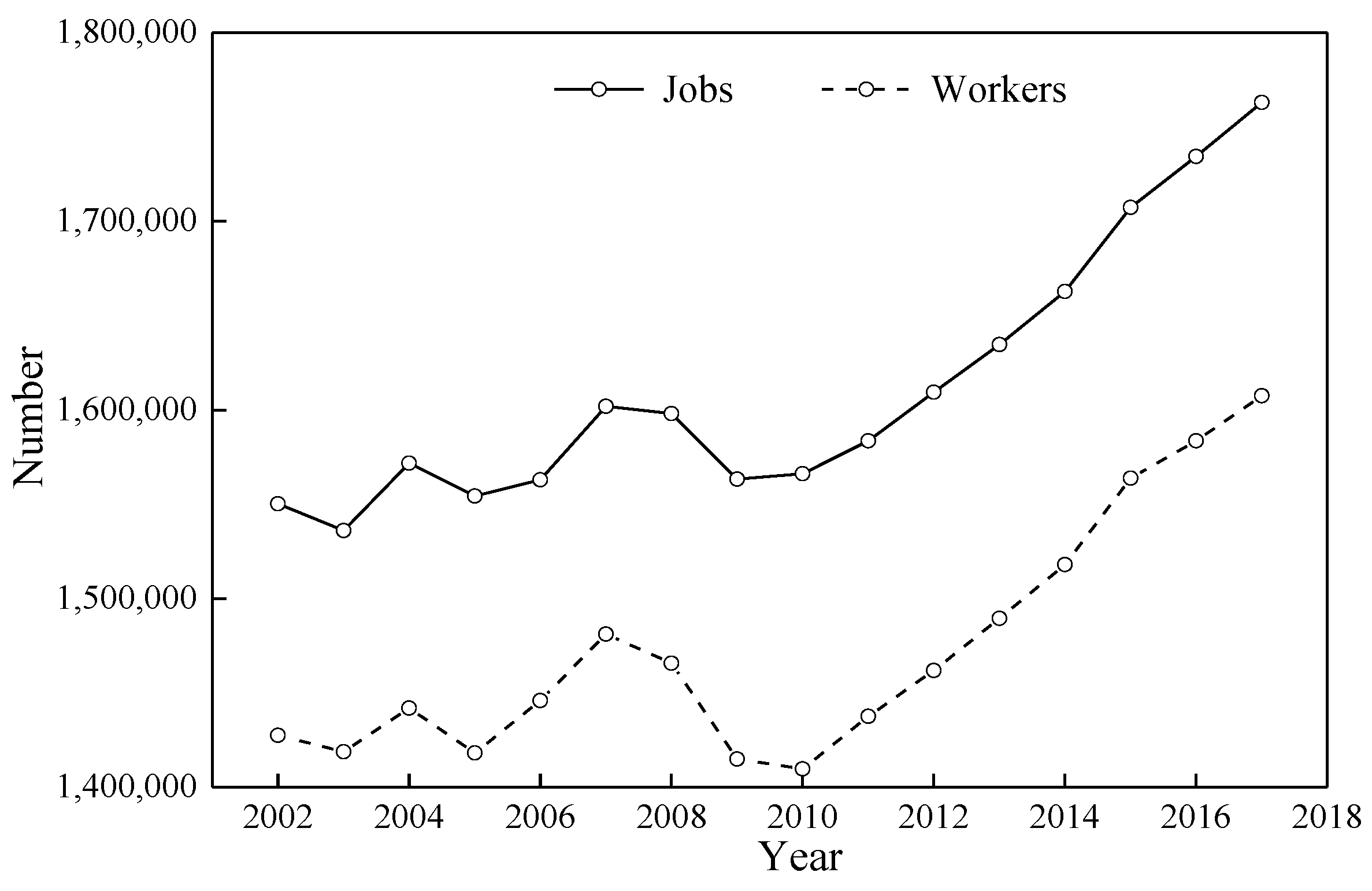
Figure 3 shows the total number of jobs and workers in the Twin Cities. A general uptrend can be clearly seen over the 14 years, indicating a growth in the economy and population; however, the downtrend from 2007 to 2009, caused by the 2008 global financial crisis, cannot be ignored. Overall, the number of jobs in the region exceeds the number of workers, both because some workers hold multiple job positions (though this cannot be told from the LEHD data) and some live outside of the Twin Cities while working inside.
This data assists in developing the correlation matrix and are useful as dependent variables in the land use regression models.
The TIGER/Line Shapefile, defined by the U.S. Census Bureau and the Metropolitan Council (2012) [41], provides selected geographic and cartographic information. The adjacency matrix can be constructed accordingly.
Further, we extracted the road network from OpenStreetMap [42], which was used to calculate the walking travel time and then the walking accessibility matrix. Specifically, the pedestrian network was constructed by eliminating the roads with “motorway”, “motorway link”, “trunk”, and “trunk link” tags. Joining it with the centroids of the census blocks, origin–destination (OD) matrix cost analysis in ArcGIS was applied to obtain the shortest walking on-road travel time between any two blocks with an assumption that the walking speed is 5 km/h [43].
The series of Access to Destinations studies provide the travel time by auto for any two blocks in the Twin Cities metropolitan area [44], which was used to construct auto accessibility matrices with different travel time thresholds.

5. Results

In this section, we display the estimation results of the land use models using data from 2002 to 2016 and discuss the performances of the three spatial weight matrices mentioned in Section 2 as well as the spatial relationship between job and worker densities.
It is worth noting that blocks with a number of jobs or workers higher than 0 for every year are selected to fit the regression models. Accessibility in different time thresholds by walking and by auto were tested, in which 30 min walking accessibility had the best fit; therefore, it was selected for comparison with the other two alternative spatial weight matrices.
The final regression results of the job and worker densities are shown in Table 1 and Table 2, respectively, in which model 1 and model 5 are the base scenarios where no spatial interaction is considered. Table 3 summarizes the elasticities calculated following Equation (7).
E = Δ Y / Y Δ X / X = d Y d X × X Y × 100 %
where:
X is an independent variable;
Y is a dependent variable.
Models that incorporate the spatial effects of the densities have a better fit than those that do not, demonstrating that the spatial interactions between densities play a role in their short-run changes. Moreover, we observed that the models which capture the spatial effects based on the correlation matrix explain the job density (model 4) and the worker density (model 8) the best; the accessibility matrix is slightly better than the adjacency matrix.
To further validate the performance of the correlation matrix, we used the three models to predict densities in 2017 and measured their predictive performances using the mean absolute percentage error (MAPE), the results of which are shown in Table 4. As expected, the models based on the correlation matrix have the highest prediction accuracy (MAPE is 6.46% for job density and 4.06% for worker density) and the lowest variation (variations of MAPE for the job and worker densities are 127.79 and 12.19, respectively). Moreover, the predictive differences among the three models are significant for job and worker densities (Friedman tests show that p = 0.000 at the 95% confidence level). Both results suggest that the land use intensity econometric model, using the correlation matrix, should be used to capture the spatial effect of land use.
The result is not surprising because the correlation matrix reflects the co-influence of various factors, including the transport network, the geographical limitations, and other factors driving the interaction of land use intensity in an implicit way, while the accessibility matrix incorporates the adjustment of the transport network to the geographical limitations, which is the only factor considered by the adjacency matrix. Note that, with regard to the computation time, the correlation matrix takes the longest, the accessibility matrix takes less, and the adjacent matrix takes the least.
An implication from the result is that micro-level land use simulation models should thoroughly consider the use of spatial interaction to describe the process of land development more precisely. A useful way to achieve this is to incorporate the correlation-based spatial weight matrix to construct transition rules describing the spatial effect.
Regarding the spatial relationships between densities, we can observe the following:
(1) job density is positively associated with the lagged change in accessible job densities, which supports the economies of agglomeration;
(2) there is a positive relationship between the worker density and the lagged changes in the adjacent and accessible job densities, demonstrating that jobs appeal to workers. This is likely because workers want to be near their work locations for a shorter commute;
(3) the effects of the lagged changes on the worker densities in the current stage of the worker density are negative and significant, both for adjacent and accessible neighbors. This means that the greater the increase in the nearby workers, the more workers move out from the location. One explanation for this is that workers want to move away from each other to reduce their fixed investment in the land.
Based on the concept of Granger-causality, i.e., that a time-series variable provides statistically significant information about another variable [45], these results indicate that a growth in jobs in nearby blocks Granger-causes a growth in the workers and jobs in the block, and that an increase in worker densities in nearby blocks Granger-causes a decrease in the worker density in the block. We imagine a scenario in which a firm has been established in a place and where other relevant firms have followed to reduce the cost of an interfirm interaction. Resident workers also followed, we suppose, to reduce their commute time. These are consistent with some of our observations about the history of the spatial development, namely, that firms arrive first, and that people follow jobs [46], suggesting a strategy with which to lower (raise) density in a region, such as, for example, for migrating firms out (in). In addition, we can infer that a city has the natural ability to overlook the fact that workers want to live away from each other.

6. Application

The change in land use intensity can be detected using the spatial regression model with the correlation matrix proposed above, which provides information on public services and infrastructure deployment. The distributions of the changes in densities from 2017 to 2022, for jobs and workers, are displayed in Table 5, in which the change is written as Equation (8).
p D U = D U , i , 2022 D U , i , 2017 D U , i , 2017 × 100 %
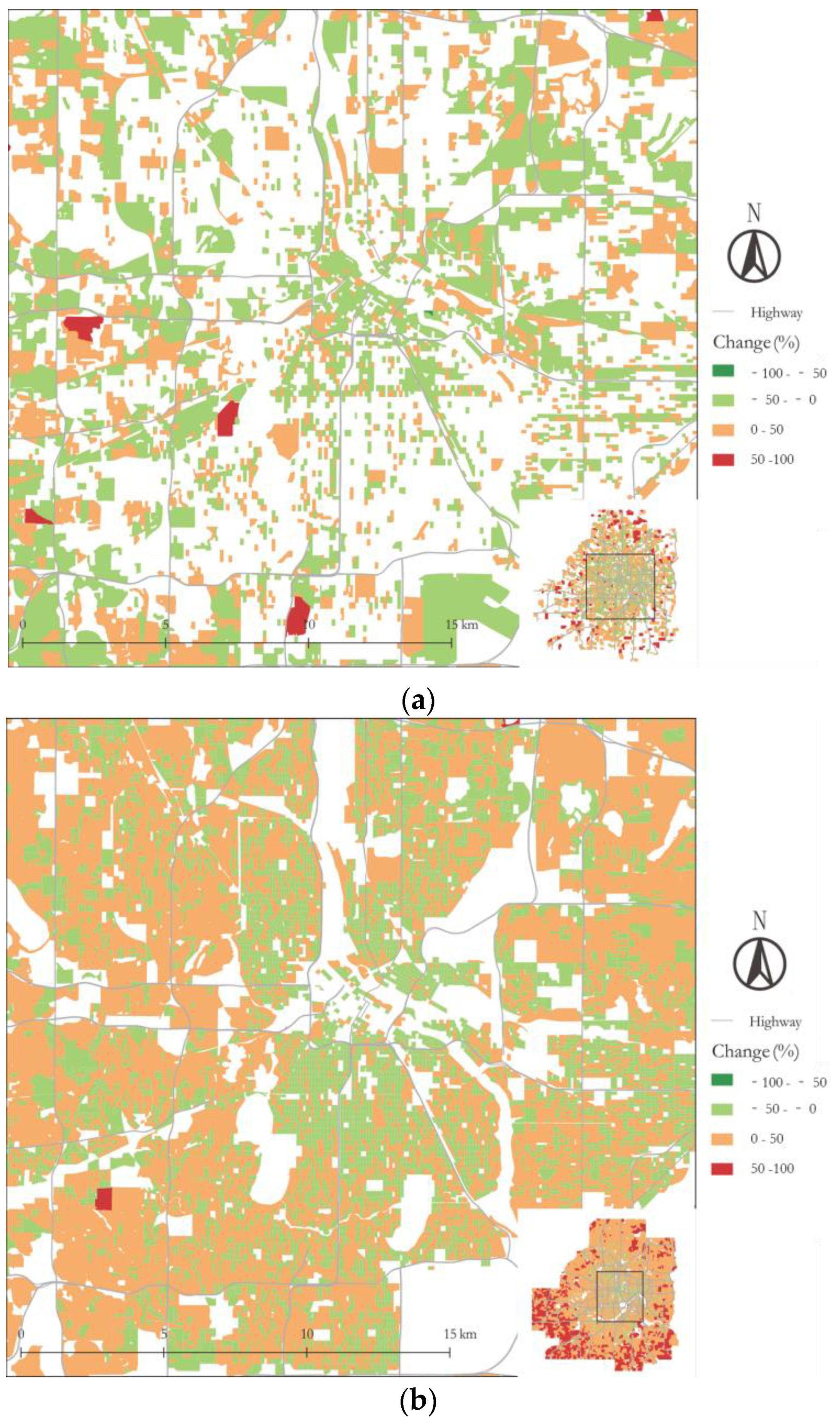
From Table 5, we can see that more than half of the blocks (56.3%) are predicted to have job density drops in 2022 compared to 2017, and that fewer (31.2%) have worker density declines. The spatial distributions of the changes are visualized in Figure 4. This information about land use intensity changes can help to determine where and how many public services or related infrastructures should be further offered so that the needs of citizens can be satisfied.

7. Conclusions

This research study aimed to determine the best way to express the variation of spatial dependency and to capture the spatial effect of land use intensity by investigating three spatial weight matrices, including the adjacency, accessibility, and correlation matrices.
The correlation matrix was calculated based on real data after temporal detrending. From this data, we found that the spatial dependencies of the job and worker densities are complementary but also competitive, similar to previous observations on traffic links [47]. Then, we validated its great performance to capture the spatial effects of densities using land use data in the Minneapolis–St. Paul region from 2002 and 2017. We also found that the accessibility matrix ranks second and that the adjacency matrix is the least helpful.
This research also discloses the cause and effect of the spatial interactions of the job and worker densities by using lagging spatial variables in regression models. The growth in jobs in nearby neighboring blocks Granger-causes the growth of workers and jobs; moreover, an increase in workers in nearby neighbor blocks Granger-causes a decrease in workers. These demonstrate the development process of a city in which some firms are established, as well as the other associated firms and workers which follow. Moreover, with an accumulation in workers in the region, some of them will move out to decrease the personal real estate costs and attain more living space. This mechanism provides insights for land use policies and can provide useful guidance for policymakers, such as suggesting the migration of firms out of (into) the region as a way to lower (raise) the density.
This study validates the good performance of a correlation matrix for land use data in a case study set in the Minneapolis–St. Paul region. In the future, data from other fields and regions can be used to further demonstrate its performance. Moreover, another direction worthy of exploration is a comparison between the performances of a machine learning model and a spatial regression model in predicting land use intensity.

Author Contributions

Conceptualization, D.L.; methodology, M.L. and D.L.; software, M.L.; validation, M.L. and M.C.; formal analysis, M.L. and D.L.; writing—original draft preparation, M.L.; writing—review and editing, M.C. and D.L.; supervision, D.L.; funding acquisition, M.L. and M.C. All authors have read and agreed to the published version of the manuscript.

Funding

This research was funded by the Fundamental Research Funds for the Central Universities, CHD, grant number 300102222105 and the Science and Technology Innovation Program of Shaanxi Province Project, grant number 2022JQ-345.

Data Availability Statement

Data that support the findings of this study are openly available at https://lehd.ces.census.gov/data/#lodes.html, accessed on 19 September 2017; https://gisdata.mn.gov/dataset/us-mn-state-metc-society-census2010tiger, accessed on 8 September 2011; http://download.geofabrik.de/north-america/us/minnesota.html, accessed on 18 July 2019; https://conservancy.umn.edu/handle/11299/200792, accessed on 9 November 2018.

Acknowledgments

This work is supported by School of Civil Engineering at the University of Sydney.

Conflicts of Interest

The authors declare no conflict of interest.

References

  1. Torrens, P.M. Simulating sprawl. Ann. Assoc. Am. Geogr. 2006, 96, 248–275. [Google Scholar]
  2. Fujita, M.; Krugman, P.; Mori, T. On the evolution of hierarchical urban systems. Eur. Econ. Rev. 1999, 43, 209–251. [Google Scholar] [CrossRef]
  3. Yeh, A.G.-O.; Li, X. A Cellular Automata Model to Simulate Development Density for Urban Planning. Environ. Plan. B Plan. Des. 2002, 29, 431–450. [Google Scholar] [CrossRef]
  4. Feng, Y.; Tong, X. Calibration of cellular automata models using differential evolution to simulate present and future land use. Trans. GIS 2018, 22, 582–601. [Google Scholar] [CrossRef]
  5. Broitman, D.; Koomen, E. Residential density change: Densification and urban expansion. Comput. Environ. Urban Syst. 2015, 54, 32–46. [Google Scholar] [CrossRef]
  6. Wang, X.; Kockelman, K.M.; Lemp, J.D. The dynamic spatial multinomial probit model: Analysis of land use change using parcel-level data. J. Transp. Geogr. 2012, 24, 77–88. [Google Scholar] [CrossRef]
  7. Shen, Y.; Silva, J.D.A.E.; Martínez, L.M. Assessing high-speed rail’s impacts on land cover change in large urban areas based on spatial mixed logit methods: A case study of Madrid Atocha railway station from 1990 to 2006. J. Transp. Geogr. 2014, 41, 184–196. [Google Scholar]
  8. Zheng, Q.; He, S.; Huang, L.; Zheng, X.; Pan, Y.; Shahtahmassebi, A.R.; Shen, Z.; Yu, Z.; Wang, K. Assessing the Impacts of Chinese Sustainable Ground Transportation on the Dynamics of Urban Growth: A Case Study of the Hangzhou Bay Bridge. Sustainability 2016, 8, 666. [Google Scholar] [CrossRef]
  9. Wrenn, D.H.; Sam, A.G. Geographically and temporally weighted likelihood regression: Exploring the spatiotemporal determinants of land use change. Reg. Sci. Urban Econ. 2014, 44, 60–74. [Google Scholar] [CrossRef]
  10. Lambin, E.F.; Geist, H.J.; Lepers, E.; Meyer, W.B.; Turner, I.B.L.; Meyfroidt, P.; Alix-Garcia, J.; Wolff, H.; Bentley, J.W.; Innes, R.; et al. Dynamics of Land-Use and Land-Cover Change in Tropical Regions. Annu. Rev. Environ. Resour. 2003, 28, 205–241. [Google Scholar] [CrossRef]
  11. Verburg, P.H.; Schot, P.P.; Dijst, M.J.; Veldkamp, A. Land use change modelling: Current practice and research priorities. GeoJournal 2004, 61, 309–324. [Google Scholar] [CrossRef]
  12. Zhou, B.; Kockelman, K.M. Neighborhood impacts on land use change: A multi-nomial logit model of spatial relationships. Ann. Reg. Sci. 2008, 42, 321–340. [Google Scholar] [CrossRef] [Green Version]
  13. Waddell, P.; Borning, A.; Noth, M.; Freier, N.; Becke, M.; Ulfarsson, G. Micro-simulation of urban development and loca-tion choices: Design and implementation of urbanism. Netw. Spat. Econ. 2003, 3, 43–67. [Google Scholar] [CrossRef]
  14. Batty, M. Cities and Complexity: Understanding Cities with Cellular Automata, Agent-Based Models and Fratals; The MIT Press: Cambridge, MA, USA, 2005. [Google Scholar]
  15. Verburg, P.H.; van Eck, J.R.R.; de Nijs, T.C.M.; Dijst, M.J.; Schot, P. Determinants of Land-Use Change Patterns in the Netherlands. Environ. Plan. B Plan. Des. 2004, 31, 125–150. [Google Scholar] [CrossRef]
  16. de Nijs, T.; Pebesma, E. Estimating the Influence of the Neighbourhood in the Development of Residential Areas in the Netherlands. Environ. Plan. B Plan. Des. 2010, 37, 21–41. [Google Scholar] [CrossRef]
  17. Levinson, D. Density and dispersion: The co-development of land use and rail in London. J. Econ. Geogr. 2007, 8, 55–77. [Google Scholar] [CrossRef]
  18. Conway, T.M. Current and Future Patterns of Land-Use Change in the Coastal Zone of New Jersey. Environ. Plan. B Plan. Des. 2005, 32, 877–893. [Google Scholar] [CrossRef]
  19. Tobler, W.R. A Computer Movie Simulating Urban Growth in the Detroit Region. Econ. Geogr. 1970, 46, 234–240. [Google Scholar] [CrossRef]
  20. Bhattacharjee, A.; Jensen-Butler, C. Estimation of the spatial weights matrix under structural constraints. Reg. Sci. Urban Econ. 2013, 43, 617–634. [Google Scholar] [CrossRef]
  21. Chung, S.; Hewings, G. Competitive and Complementary Relationship between Regional Economies: A Study of the Great Lake States. Spat. Econ. Anal. 2015, 10, 205–229. [Google Scholar] [CrossRef]
  22. Ermagun, A.; Levinson, D.M. Development and application of the network weight matrix to predict traffic flow for congested and uncongested conditions. Environ. Plan. B Urban Anal. City Sci. 2018, 46, 1684–1705. [Google Scholar] [CrossRef]
  23. Getis, A.; Aldstadt, J. Constructing the spatial weight matrix using a local statistic. Geogr. Anal. 2004, 36, 90–104. [Google Scholar] [CrossRef]
  24. Feld, L.P.; Köhler, E.A.; Wolfinger, J. Modeling fiscal sustainability in dynamic macro-panels with heterogeneous effects: Evidence from German federal states. Int. Tax Public Financ. 2019, 27, 215–239. [Google Scholar] [CrossRef]
  25. Asumadu, S.S.; Vladimir, S. Effect of foreign direct investments, economic development and energy consumption on greenhouse gas emissions in developing countries. Sci. Total Environ. 2019, 646, 862–871. [Google Scholar]
  26. Iacono, M.; Levinson, D.; El-Geneidy, A. Models of Transportation and Land Use Change: A Guide to the Territory. J. Plan. Lit. 2008, 22, 323–340. [Google Scholar] [CrossRef]
  27. Anselin, L. Spatial econometrics: Methods and models. J. Am. Stat. Assoc. 1988, 85, 905–907. [Google Scholar]
  28. Alijani, Z.; Hosseinali, F.; Biswas, A. Spatio-temporal evolution of agricultural land use change drivers: A case study from Chalous region, Iran. J. Environ. Manag. 2020, 262, 110326. [Google Scholar] [CrossRef]
  29. Wyman, M.S.; Stein, T.V. Modeling social and land-use/land-cover change data to assess drivers of smallholder defor-estation in Belize. Appl. Geogr. 2010, 30, 329–342. [Google Scholar] [CrossRef]
  30. Iacono, M.; Levinson, D. Predicting land use change: How much does transportation matter. Transp. Res. Rec. 2009, 2119, 130–136. [Google Scholar] [CrossRef]
  31. Cui, M.; Levinson, D. Accessibility and the Ring of Unreliability. Transp. A Transp. Sci. 2016, 14, 4–21. [Google Scholar] [CrossRef]
  32. Vickerman, R.W. Accessibility, Attraction, and Potential: A Review of Some Concepts and Their Use in Determining Mobility. Environ. Plan. A Econ. Space 1974, 6, 675–691. [Google Scholar] [CrossRef]
  33. Wachs, M.; Kumagai, T. Physical accessibility as a social indicator. Socio-Econ. Plan. Sci. 1973, 7, 437–456. [Google Scholar] [CrossRef]
  34. Abdi, H. The kendall rank correlation coefficient. In The Concise Encyclopedia of Measurement and Statistics; Springer: New York, NY, USA, 2008. [Google Scholar]
  35. Cohen, I.; Huang, Y.; Chen, J.; Benesty, J. Pearson Correlation Coefficient. In Noise Reduction in Speech Processing; Springer: Berlin/Heidelberg, Germany, 2009. [Google Scholar]
  36. Aldstadt, J.; Getis, A. Using AMOEBA to Create a Spatial Weights Matrix and Identify Spatial Clusters. Geogr. Anal. 2006, 38, 327–343. [Google Scholar] [CrossRef]
  37. Jönsson, K. Cross-sectional and serial correlation in a small-sample homogeneous panel data unit root test. Appl. Econ. Lett. 2005, 12, 899–905. [Google Scholar] [CrossRef]
  38. Hoechle, D. Robust Standard Errors for Panel Regressions with Cross-Sectional Dependence. Stata J. Promot. Commun. Stat. Stata 2007, 7, 281–312. [Google Scholar] [CrossRef]
  39. Driscoll, J.C.; Kraay, A.C. Consistent Covariance Matrix Estimation with Spatially Dependent Panel Data. Rev. Econ. Stat. 1998, 80, 549–560. [Google Scholar] [CrossRef]
  40. Longitudinal Employer-Household Dynamics. Available online: https://lehd.ces.census.gov/data/#lodes.html (accessed on 19 September 2017).
  41. Census 2010 Geography—Blocks, Block Groups, Tracts, Tazs, Counties, County Subdivisions and Water. Available online: https://gisdata.mn.gov/dataset/us-mn-state-metc-society-census2010tiger (accessed on 8 September 2011).
  42. Geofabrik. Minnesota, 2012. Available online: http://download.geofabrik.de/north-america/us/minnesota.html (accessed on 18 July 2019).
  43. Murphy, B.; Levinson, D.; Owen, A. Accessibility and Centrality Based Estimation of Urban Pedestrian Activity. Working Papers: 2015, Minneapolis, USA. Available online: https://hdl.handle.net/11299/179834 (accessed on 18 July 2019).
  44. Accessibility Measures to Population, Employment and Labour by Auto and Transit for the Period of 1995, 2000, 2005, 2010 for the Twin Cities Region. Available online: https://conservancy.umn.edu/handle/11299/200792 (accessed on 9 November 2018).
  45. Granger, C.W.J. Investigating Causal Relations by Econometric Models and Cross-spectral Methods. Econometrica 1969, 37, 424–438. [Google Scholar] [CrossRef]
  46. Storper, M. Why do regions develop and change? The challenge for geography and economics. J. Econ. Geogr. 2010, 11, 333–346. [Google Scholar] [CrossRef]
  47. Ermagun, A.; Levinson, D. An Introduction to the Network Weight Matrix. Geogr. Anal. 2017, 50, 76–96. [Google Scholar] [CrossRef]
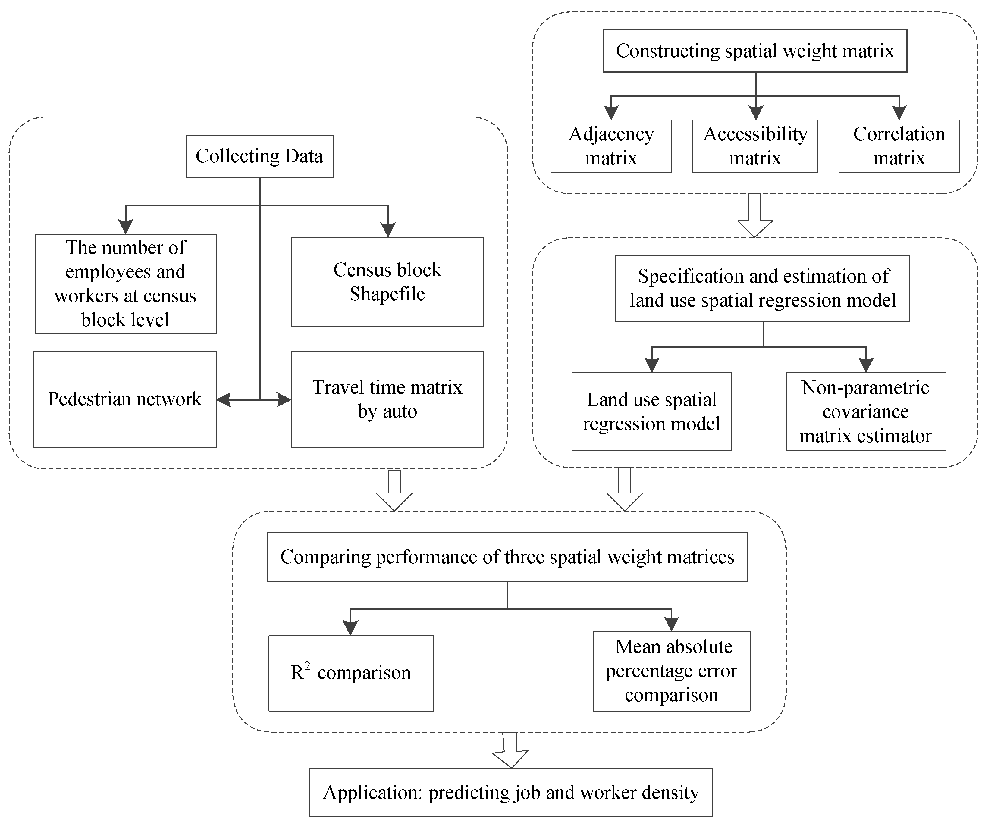
Figure 1. Framework.
Urbansci 07 00022 g001
Figure 2. Sample blocks for constructing spatial weight matrices.
Urbansci 07 00022 g002
Figure 3. Trend in total number of jobs and workers in the Twin Cities.
Urbansci 07 00022 g003
Figure 4. Spatial distributions of density changes between 2022 and 2017 for the Twin Cities: (a) change in job density; (b) change in worker density.
Urbansci 07 00022 g004
Table 1. Predicting job density based on three different spatial matrices.
Variables ln ( D e , i , t )
Model 1Model 2Model 3Model 4
Coef.Drisc/Kraay Std. Err.Sig.Coef.Drisc/Kraay Std. Err.Sig.Coef.Drisc/Kraay Std. Err.Sig.Coef.Drisc/Kraay Std. Err.Sig.
ln ( D e , i , t 5 ) 9.12 × 10−012.61 × 10−03***9.12 × 10−012.32 × 10−03***9.11 × 10−012.81 × 10−03***9.42 × 10−011.13 × 10−02***
W n ln D e , i , t 5 D e , i , t 10 3.68 × 10−035.46 × 10−03
W n ln D w , i , t 5 D w , i , t 10 1.32 × 10−031.22 × 10−02
W a ln D e , i , t 5 D e , i , t 10 3.22 × 10−034.59 × 10−04**
W a ln D w , i , t 5 D w , i , t 10 −1.00 × 10−038.26 × 10−04
W c ln D e , i , t 5 D e , i , t 10 4.08 × 10−041.29 × 10−05***
W c ln D w , i , t 5 D w , i , t 10 2.98 × 10−052.88 × 10−05
Const.9.12 × 10−012.61 × 10−03***9.12 × 10−012.32 × 10−03***9.11 × 10−012.81 × 10−03***9.42 × 10−011.13 × 10−02***
Obs.49,26049,26049,26049,260
Group8210821082108210
Prob > F0.0000.0000.0000.000
R20.79430.79430.79440.8969
*** p < 0.001, ** p < 0.01, * p < 0.05.
Table 2. Predicting worker density based on three different spatial matrices.
Variables ln ( D w , i , t )
Model 5Model 6Model 7Model 8
Coef.Drisc/Kraay Std. Err.Sig.Coef.Drisc/Kraay Std. Err.Sig.Coef.Drisc/Kraay Std. Err.Sig.Coef.Drisc/Kraay Std. Err.Sig.
ln ( D w , i , t - 5 ) 8.94 × 10−011.54 × 10−02***8.93 × 10−011.67 × 10−02***8.84 × 10−011.33 × 10−02***9.36 × 10−018.70 × 10−03***
W n ln D e , i , t 5 D e , i , t 10 9.75 × 10−033.68 × 10−03*
W n ln D w , i , t 5 D w , i , t 10 −2.82 × 10−024.33 × 10−03**
W a ln D e , i , t 5 D e , i , t 10 2.18 × 10−033.60 × 10−04**
W a ln D w , i , t 5 D w , i , t 10 −3.86 × 10−031.64 × 10−04***
W c ln D e , i , t 5 D e , i , t 10 2.80 × 10−041.97 × 10−05***
W c ln D w , i , t 5 D w , i , t 10 1.26 × 10−053.86 × 10−05
Const.−8.36 × 10−011.52 × 10−01**−8.53 × 10−011.59 × 10−01**−9.46 × 10−011.26 × 10−01**−4.45 × 10−018.08 × 10−02**
Obs.49,260 202,230 202,230 202,230
Group8210 33,705 33,705 33,705
Prob > F0.000 0.000 0.000 0.000
R20.8035 0.8045 0.8058 0.9027
*** p < 0.001, ** p < 0.01, * p < 0.05.
Table 3. Elasticities for job and worker densities.
Variables D e , i , t
25 Percentile50 Percentile75 Percentile
−9.730−7.764−6.453
ValueElasticityValueElasticityValueElasticity
W a ln D e , i , t 5 D e , i , t 10 2.631 0.003 −0.087 2.796 0.003 −0.116
W c ln D e , i , t 5 D e , i , t 10 −1274.180 0.000 5.344 −1752.130 0.000 9.210
Variables D w , i , t
25 Percentile50 Percentile75 Percentile
−8.113−7.437−6.974
ValueElasticityValueElasticityValueElasticity
W n ln D e , i , t 5 D e , i , t 10 0.061 0.010 −0.007 −0.182 0.010 0.024
W n ln D w , i , t 5 D w , i , t 10 −0.132 −0.028 −0.046 −0.389 −0.028 −0.147
W a ln D e , i , t 5 D e , i , t 10 −0.058 0.002 0.002 3.309 0.002 −0.097
W a ln D w , i , t 5 D w , i , t 10 −1.091 −0.004 −0.052 −0.055 −0.004 −0.003
W c ln D e , i , t 5 D e , i , t 10 −826.985 0.000 2.856 −5.490 0.000 0.021
Table 4. Predictive performances of three different spatial matrices.
Spatial MatricesJob DensityWorker Density
MAPEVarianceFriedman TestMAPEVarianceFriedman Test
Adjacency8.10190.480.0004.2715.220.000
Accessibility8.09190.824.1615.00
Correlation6.46127.794.0612.19
Table 5. The distribution of density changes between 2017 and 2022.
Change (%)−100–−50−50–00–5050–100
Density
Job 0.0000.5630.4220.015
Worker 0.0000.3120.6710.017
Disclaimer/Publisher’s Note: The statements, opinions and data contained in all publications are solely those of the individual author(s) and contributor(s) and not of MDPI and/or the editor(s). MDPI and/or the editor(s) disclaim responsibility for any injury to people or property resulting from any ideas, methods, instructions or products referred to in the content.