The “Paris-End” of Town? Deriving Urban Typologies Using Three Imagery Types

Abstract

Urban typologies allow areas to be categorised according to form and the social, demographic, and political uses of the areas. The use of these typologies and finding similarities and dissimilarities between cities enables better targeted interventions for improved health, transport, and environmental outcomes in urban areas. A better understanding of local contexts can also assist in applying lessons learned from other cities. Constructing urban typologies at a global scale through traditional methods, such as functional or network analysis, requires the collection of data across multiple political districts, which can be inconsistent and then require a level of subjective classification. To overcome these limitations, we use neural networks to analyse millions of images of urban form (consisting of street view, satellite imagery, and street maps) to find shared characteristics between the largest 1692 cities in the world. The comparison city of Paris is used as an exemplar and we perform a case study using two Australian cities, Melbourne and Sydney, to determine if a “Paris-end” of town exists or can be found in these cities using these three big data imagery sets. The results show specific advantages and disadvantages of each type of imagery in constructing urban typologies. Neural networks trained with map imagery will be highly influenced by the structural mix of roads, public transport, and green and blue space. Satellite imagery captures a combination of both urban form and decorative and natural details. The use of street view imagery emphasises the features of a human-scaled visual geography of streetscapes. However, for both satellite and street view imagery to be highly effective, a reduction in scale and more aggressive pre-processing might be required in order to reduce detail and create greater abstraction in the imagery.

1. Introduction

The form a city takes and the way land is allocated can have both positive and negative consequences for population health and well-being. For example, cities with compact forms have been found to lead to better health outcomes [1,2,3] and reductions in per capita emissions [4]. City design can also be a factor in encouraging or discouraging the uptake of active transport [5] leading to better health outcomes [6] or locking-in car dependency [7], increasing levels of air pollution [8], obesity [9], and road trauma [10]. Due to the long time scales of urban change and the high stability of city structures [11], we must consider current cities as both a snapshot in time but also a culmination of years of construction. Policy-makers and urban/transport planners have an opportunity to embrace strategies that proactively support safe active transport modes as facilitated by urban designs witnessed in some countries around the world. However, the rigid structure of cities makes rapid changes difficult and changes should be undertaken with due care, as the impacts will be very long-lived [12,13]. Planning for change requires methods that can objectively compare cities while also accounting for local context, so as to understand the associations between urban design features, transport networks, and environmental outcomes.

Urban typologies allow a city to be “read”, linking the urban morphological form with the social, demographic, and political uses of these spaces [14]. These grew from a theoretical basis, examining the division of a city as well as the cities themselves as artefacts [15]. Krier [16] endeavoured to quantify how urban space typologies could be derived, starting with basic geometric shapes (squares, triangles, and circles), their distortions, and then their combination into composite street plans. Typologies are also influenced by an urban area’s original development and later growth. Rossi [15] traced city development in the Americas through two main starting points. Cities in Latin America and New York City were based on a grid system (influenced by the Laws of the Indies [17]), while the stereotypical Old West town originated as a main street village. Urban development evolved as cities outgrew their (now obsolete) city walls and adapted to the industrial revolution [16]. Other theoretical typologies considered different urban elements and scales. Argan and Rykwert [18] defined a number of typologies based on different levels—an urban scale (the configurations of buildings), a building scale (the constructed elements), and a detailed scale (the decorative elements on buildings). These theoretical typologies more often described morphology rather than function.

In order to derive function-based typologies, a number of methods have been devised. Harris [19] used occupational and employment figures to determine a city’s most important economic activity (such as manufacturing, retail, or tourism). Other studies used economic activity data to find similar sorts of functional typologies [20]. Finally, Bruce and Witt [21] used a range of city statistics to group cities into clusters. While these typologies can discover a city’s main functional use, they say nothing of a city’s urban design and its potential impact on residents’ movement patterns or modes.

Contemporary Approaches

New methods to define city typologies emerged in the 1980s and 90s with the growing availability of databases of spatial data and increased computing power. Much of this work focused on road infrastructure in cities, and drew from the structural sociology field, in which groups of people were represented as part of a broader network structure. The “space syntax” of Hillier [22] established a correlation between configurations of urban forms and variations of human interactions within it. Other recent remote-sensing-based methods depart from the pure network analysis methods to derive urban typologies. Nighttime light data has been used to categorise cities into stages of urbanisation and levels of economic activities [23]. Urban metrics (road geometry, building dimensions and heights, and vegetation heights) have also been used to classify cities into typologies of differing periods of historical design and urban planning (i.e., 19th Century, 1950s, 1970s, etc.) [24]. Local climate zones (LCZ) enable urban climate modelling parametrisations using metrics of building heights, street widths, and surface types fractions to classify urban areas [25,26].

Building on recent advances in computing power, artificial intelligence, and urban imagery, new approaches have been created to discover unique visual characteristics of cities and how they are used. For example, large numbers of geo-tagged photos have been used to detect patterns of urban usage and public perception of a number of areas’ functional and social attributes [27,28]. Place Pulse, a database of urban imagery using crowd-sourced classifications (including safety, beauty, and liveliness) has been built to quantify perceptions of urban areas [29,30] and inequality [31]. Doersch et al. [32] used a large number of geo-localised street-level images to discover common visual features across a number of cities.

Still, most methods described above require some amount of subjective classification of local input data, the quality and availability of which can vary widely across collection or political districts. We propose to overcome these limitations by using neural networks to find similarities in imagery of urban areas from Google and Baidu. This imagery offers universal coverage of satellite imagery and maps and nearly universal coverage of street view imagery. In addition, it provides a high consistency for map imagery (except in the case of South Korea), and street view imagery is captured using a common methodology and equipment set. This work grows from a series of projects intended to overcome these limitations by utilising a range of different types of imagery to allow analysis of urban design at a global scale. The first trains neural networks to recognise specific cities with digital street map images and to find clusters of city types and attribute the urban design’s contribution to road trauma [10]. A second extracts block-scale metrics from maps to locate neighbourhood types [33]. Expanding on those works in this paper, we also use street view and satellite imagery, in addition to the map imagery, to train neural networks. Paris, France is an iconic international city [34] with widely recognisable visual elements [32], leading many cities (including Melbourne and Sydney) to claim that they have a "Paris-end" of town [35], or are a “Paris on the [insert name of local river]” [36] (e.g., “Paris on the Yarra”). To illustrate the advantages and disadvantages of each imagery type, we therefore use the comparison city of Paris as an exemplar. We perform a case study using two Australian cities, Melbourne and Sydney, and determine if a “Paris-end” of town exists or can be found in these cities using three different types of imagery datasets, as well as determine what scales are most appropriate with these datasets to find typologies and what types of features are best suited towards a particular research question.

2. Methods

2.1. Neural Network

The methods applied in this study are based on artificial intelligence, and in particular deep neural networks [37,38,39]. Neural network architectures that have proven to be particularly successful at image recognition tasks are convolutional neural networks [40]. The model for image recognition used in this study is based on the Inception V2 architecture [41,42].

2.2. Imagery Sampling

The concept employed in this study was to train a model to correctly recognise individual cities based on examples of different types of urban imagery (street maps, satellite remote sensing, and street view images). The resulting model could then make predictions as to where entirely new images it was presented with were from. Specifically, the assumption was that if presented with an image of a city that was not Paris but the model “thought” that it was, then the sample city image presumably contained features that were “Paris-like” in nature.

A total of 1692 cities with populations of >300,000 people were initially selected for analysis [43]. Data from Google Maps and Baidu Maps were used to identify the urban form for each city in a globally consistent framework. The sampling area for each city was chosen as a circular area aligned to the city’s centre (as specified by United Nations [43]), where the radius r (km) of the sampling area was determined based on the population size p according to Barthelemy [44]:

$$r=\sqrt{\frac{28.27}{\pi }{\left(\frac{p}{300,000}\right)}^{0.85}}$$

(1)

Having identified individual cities, a two-stage sampling approach was applied. As no standardised urban boundaries are available for all the cities evaluated in this study (and methods to define urban boundaries are still an open research question [45,46,47,48,49]), we developed the following methodology. Firstly, a sampling area extending 1.5 km from the identified city centroid [43] was set as a baseline. As sample cities’ populations increased in size, the sampling area increased by a power of 0.85 to the proportional increase in population size [44]. Standardising the sampling area in this manner avoided socio-political discrepancies relating to a city’s “true” boundary and captured differences in population density and shape between small (e.g., Wellington, New Zealand; Izmit, Turkey) and global mega-cities (e.g., Tokyo, Japan; Delhi, India). Location sampling areas were adjusted for the earth’s curvature [50]. Large waterbodies (e.g., oceans but not coastlines) were removed from the sampling area, as they were not indicative of urban form.

These procedures result in a population and waterbody-adjusted circular area centred on the city’s central coordinates, capturing the widest extent of each city while minimising the amount of non-urban locations.

2.3. Imagery Sources

Three neural networks (see

Table 1. Neural networks trained and evaluated in this study.

Abbreviation	Imagery Source
GM	Google Static Maps, image type of “map”
GS	Google Static Maps, image type of “satellite”
GSV-BSV	Google Street View/Baidu Street View

) were trained using street maps, satellite imagery, and street view imagery from each city. Images were downloaded from each of the following sources, using the appropriate application programming interface (API), and were randomly sampled for each city and each network. Imagery from Sydney and Melbourne was excluded as they were included in the evaluation dataset. All imagery was downloaded from April to August 2017 using the latest imagery available from each.

The first neural network (referred to as GM) used Google Maps images as training material. Images were sized 256 × 256 pixels using a zoom level of 16 (approximately 400 × 400 m). These were obtained from the selected locations using a custom style defined with the Google Static Maps API [51] (see Figure 1a for an example of Paris, France). The images provide a high-level abstraction of road (black) and public transport (orange) networks, green space (green), and water bodies (blue). Any remaining space is coded white. Due to mapping inconsistencies in South Korea, all 25 South Korean cities were removed from the dataset, reducing the number of cities to 1665. One thousand training images were used per city (for this neural network as well as the following two), for a total dataset of 1,665,000 images in 1665 classifications.

The second neural network (referred to as GS), used Google Maps satellite imagery obtained through the Google Static Maps API [51]. Google Maps satellite imagery is a mosaic of cloud-free imagery from multiple sources and acquisition times. Originally based on Landsat 7 imagery, this has largely been replaced by Landsat 8 since 2013 and has a 15 m/pixel resolution [53]. The majority of the imagery we used dates from March and April 2017, with the rest from 2016 and early 2017. A few locations (such as Iraq and Afghanistan) date back as far as 2010. Image type was set to “satellite” using a zoom level of 16 (approximately 400 × 400 m) and image size of 256 × 256. Suitable imagery was not available for two cities, bringing the number of cities to 1688 (also excluding Melbourne and Sydney) and a total dataset of 1,688,000 images. Figure 1b shows a sample image, from Adelaide, Australia.

The third neural network (referred to as GSV-BSV) used street view imagery obtained through a combination of Google Street View (GSV) [52] and Baidu Maps Street View (BSV) [54]. Google updates their imagery periodically over a number of years. The imagery we used was approximately split across the following time periods: 35% 2016, 20% 2015, 15% 2014, 5% 2012, 10% 2011, and 15% including the remaining years back to 2007. Baidu street view imagery has a similar distribution and update patterns, but its oldest imagery only dates back to 2013. One thousand images each were sampled for the 1074 cities for which imagery was available (a total of 1,074,000 images) at a 256 × 256 resolution, a pitch of 0, a field of view of 90 degrees, and a random heading from 0 to 359 degrees. Random headings were used to give the imagery the widest range of samples of the urban areas and ensure that the heading itself didn’t influence the training (i.e., grid street systems always orientated in the same direction resulting in cities only sampling up and down the centre of streets). Images inside tunnels, indoor locations, dark locations, or otherwise unusable images were removed and replaced by resampling.

No street view imagery of China was available through GSV, so BSV was used instead. In order to minimise the differences between the two data sources and to minimise strong country-specific items (e.g., text on road signs) influencing neural network training, further image processing was performed to segment each image before use in training and evaluation. The Python module pymeanshift [55] was used to segment each image (using a spatial radius of 6, range radius of 4.5, and minimum density of 50). The effect of mean shift segmentation is to reduce the detail in images by replacing clusters of nearby pixels of similar colours with the mean value of those colors. Figure 1c shows an example of an image (from Sydney, Australia), after the mean shift pre-processing step of an original GSV image, used for the GSV-BSV training process.

Images from Sydney and Melbourne, Australia were excluded from the training data and were instead used for evaluation. These evaluation data were sampled using a grid at locations 400 m apart across the greater metropolitan areas, with 23,027 possible locations for Melbourne and 24,596 for Sydney using the same API methods and at the same scales and resolutions described above for the training data. Availability of imagery for GSV at these locations was 59.5% and 91.1%, respectively. The sampled Melbourne area contained a much higher percentage of rural areas without roads (the primary location for GSV imagery) than the sampled Sydney area.

2.4. Neural Network Training

The Inception V2 network was used in this study and the three networks (GM, GS, and GSV-BSV) were trained with 256 × 256 sized imagery. The Inception network was calibrated using supervised learning, using the city names as class labels, to enable the generated dataset to identify the name of the city based on a supplied image. Several pre-processing steps were performed before supplying the image to the neural network. Images were randomly cropped from 256 × 256 × 3 to Inception V2’s native 224 × 224 × 3 resolution. No zooming was applied, the aspect ratio was kept fixed, and colour transformations were not used. All images were normalised to [−1, 1] by subtracting a colour value of 128 from each pixel and multiplying by 1/128. To ensure good mixing, training images were randomly allocated to batches. Validation images (25% of the 1000 training images for each city were reserved as validation data) were transformed to 224 × 224 × 3 using central cropping.

To update weights in the neural network, a loss function was specified to quantify the extent of any current misclassifications, namely the cross entropy calculated on the softmax layer. Model parameters were calibrated by minimising this loss function using stochastic gradient descent with a Nesterov momentum of 0.9. Other parameters included a batch size of 64 samples, reducing learning rate starting at 0.9 per batch, batch normalisation, a dropout rate of 0.2 after the final average-pooling operations, and an L2 regularisation weight per sample of 0.0001. Each model was trained until convergence for a total of 150 epochs, using the Microsoft Cognitive Toolkit (CNTK) [56].

2.5. Neural Network Inference

Using the three trained models, inferences were performed using the evaluation datasets for Melbourne and Sydney. As Melbourne and Sydney are not present in the training data, the neural network was forced to choose the city with the most similar characteristics for each of the sampled locations. Using these predictions, every location in both cities was determined to be “most like” another world city from the list due to characteristics contained within the street map, satellite, or street-view image. The neural network will calculate probabilities that an image belongs in each classification (the city name) for each image in the dataset. We filtered out individual locations in the following results where the highest ranked probability was lower than 50%.

3. Results

Using 25% of the training data, validation was performed on each model. The neural network models for Google Maps (GM), Google Satellite maps (GS), and Google Street View/Baidu Street view (GSV-BSV) reached a final accuracy of 73.2% (top five: 85.0%), 99.4% (top five: 99.97%), and 43.1% (top five: 69.8%), respectively. These accuracies were calculated at the end of each epoch during the training step, testing the neural network’s skill in correctly identifying the correct city out of the nearly 1700 cities (excluding Melbourne and Sydney).

The resulting predictions from model inference of the evaluation data were analysed in various ways. First, the top 20 predicted cities for the evaluation points for each imagery dataset were calculated (see

Table 2. Top 20 cities similar to Melbourne and Sydney. The table shows the percentage of evaluated locations predicted to be a certain city for GM, GS, and GSV-BSV neural networks.

(a). GM
Predicted City	Mel %	Syd %
Brisbane, AUS	13.0	7.9
Beer Sheva, ISR	5.3	11.0
Canberra, AUS	2.6	5.7
Sunshine Coast, AUS	2.3	0.7
McAllen, USA	2.1	0.3
Valparaíso, CHL	1.0	0.7
Haifa, ISR	0.8	1.6
Gold Coast, AUS	0.8	0.5
Pretoria, ZAF	0.6	-
Newcastle, AUS	0.6	2.6
Toronto, CAN	0.6	0.4
Auckland, NZL	0.5	0.6
Perth, AUS	0.5	-
Johannesburg, ZAF	0.4	-
Philadelphia, USA	0.4	-
Jerusalem, ISR	0.2	0.8
Port Elizabeth, ZAF	0.3	-
Washington, D.C., USA	0.2	-
Southend-On-Sea, GBR	0.2	-
Virginia Beach, USA	-	0.4
London, GBR	-	0.3
Barcelona, ESP	-	0.3
Adelaide, AUS	-	0.3
Tasikmalaya, IDN	-	0.3
Douala, CMR	-	0.2
Hardwar, IND	-	0.2
(b). GS
Predicted city	Mel %	Syd %
Jundiaí, BRA	7.8	10.6
Wellington, NZ	4.1	0.09
Campinas, BRA	2.4	4.0
Miami, USA	2.2	-
Adelaide, AUS	1.7	-
Provo-Orem, USA	1.3	-
Macapá, BRA	0.6	-
Gold Coast, AUS	0.5	-
Rosario, ARG	0.4	1.1
Qitaihe, CHN	0.4	-
Johannesburg, ZAF	0.4	0.05
Buenos Aires, ARG	0.3	-
Canberra, AUS	0.2	-
Mendoza, ARG	0.2	-
Juiz De Fora, BRA	0.2	0.8
Pulandian, CHN	0.2	-
Newcastle, AUS	0.2	0.2
Palma, ESP	0.2	0.08
Cape Town, ZAF	0.2	-
Sevastopol, UKR	-	4.7
Memphis, USA	-	0.6
Baaqoobah, IRQ	-	0.4
Belgaum, IND	-	0.2
Qazvin, IRN	-	0.2
Nagasaki, JPN	-	0.1
New Orleans, USA	-	0.1
Malaga, ESP	-	0.1
Guayaquil, ECU	-	0.07
Khabarovsk, RUS	-	0.06
Chiinu, MDA	-	0.05
(c). GSV-BSV
Predicted city	Mel %	Syd %
Sunshine Coast, AUS	4.0	5.0
Perth, AUS	4.0	1.6
Adelaide, AUS	4.0	1.2
Auckland, NZL	2.7	0.8
Canberra, AUS	1.9	3.1
Newcastle, AUS	1.7	3.1
Gold Coast, AUS	1.3	3.3
Christchurch, NZL	0.9	-
Brisbane, AUS	0.8	3.2
Bonita Springs, USA	0.7	0.5
Stockton, USA	0.7	0.5
Curitiba, BRA	0.7	0.4
Cape Town, ZAF	0.7	0.4
Concord, USA	0.6	0.3
East London, ZAF	0.5	0.4
West Yorkshire, GBR	0.5	-
Teeside, GBR	0.4	-
Los Angeles, USA	0.4	-
Montevideo, URY	0.3	-
San Diego, USA	-	0.9
Jacksonville, USA	-	0.4
Vereeniging, ZAF	-	0.4
Virginia Beach, USA	-	0.4
McAllen, USA	-	0.4

for GM, GS, and GSV-BSV).

3.1. Top 20 Predicted Cities

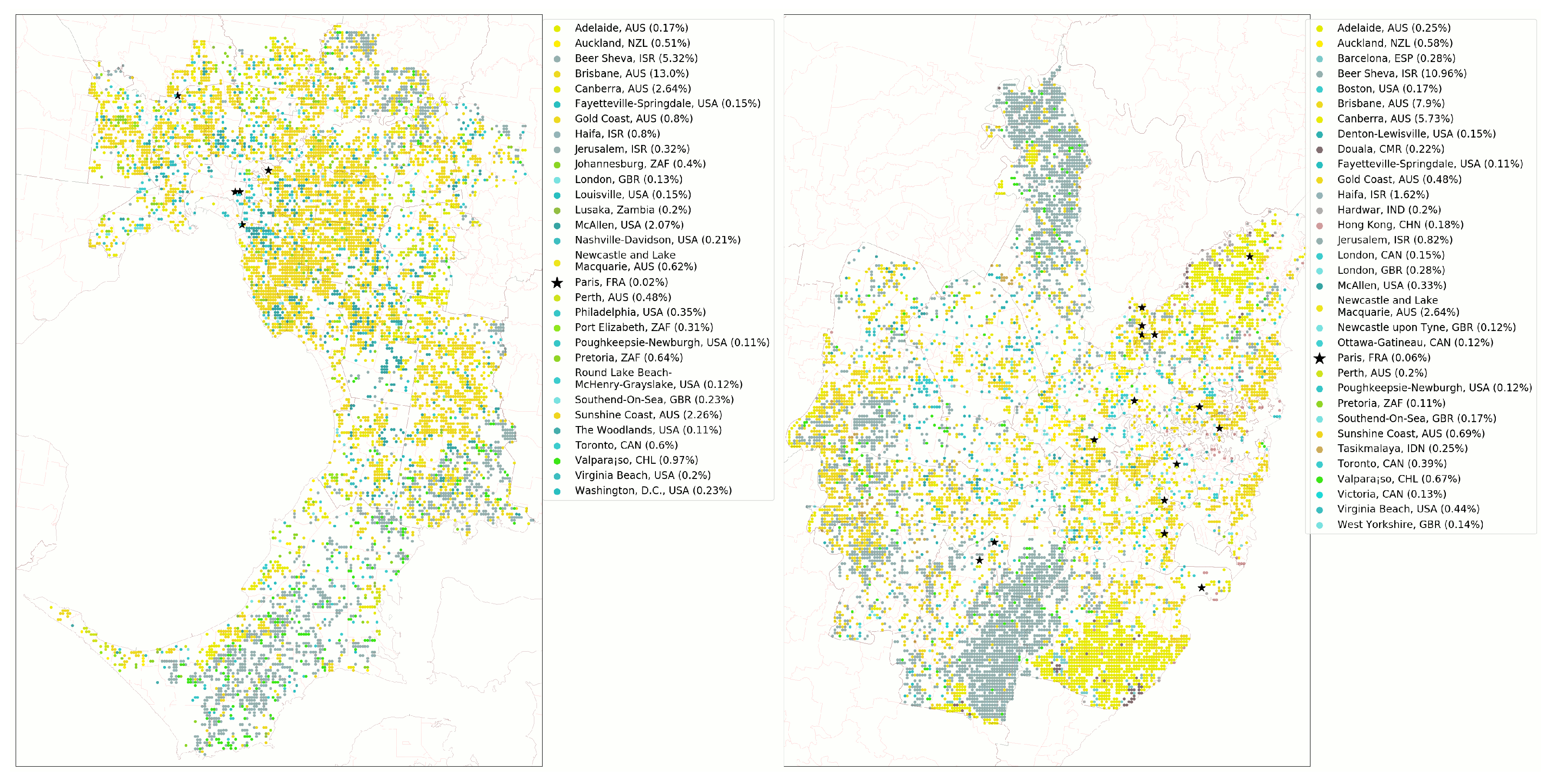
The GM (map view) neural network predictions (Table 2a) are dominated by other Australian cities (Brisbane, Canberra, Sunshine Coast, Gold Coast, Newcastle and Lake Macquarie, Perth, and Adelaide) as well as a number of cities from Israel, South Africa, and the United States. Alternative Australian cities make up nearly 20% of the top 20 predictions for Melbourne and 17% for Sydney. Melbourne and Sydney also show strong similarities with each other with the neural network considering them similar to the same 12 cities out of the top 20 predictions.

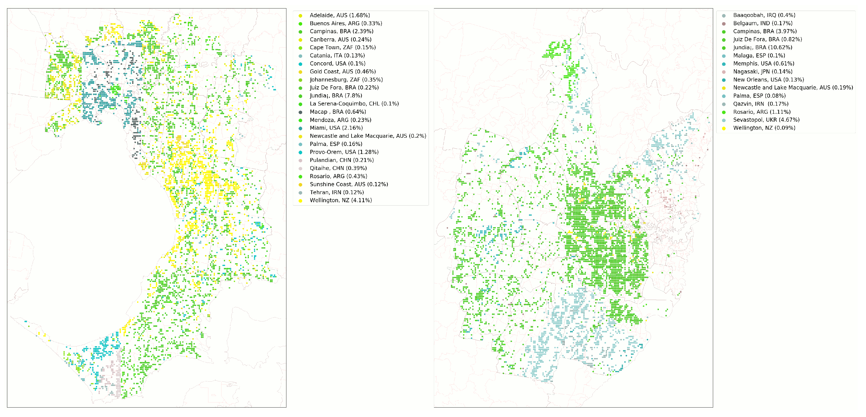
The GS (satellite view) neural network predictions (Table 2b) show wider divergences from other Australian cities and between Melbourne and Sydney themselves, with both often matched to Brazilian cities. Melbourne is matched to Brazil in 11% of the evaluation locations while Sydney is matched to Brazilian cities in 15%. Melbourne and Sydney show wider divergences from each other using the GS network in comparison to the GM network, only having 8 of the top 20 predicted cities in common. In diverging predictions, 4.1% of Melbourne is confused with Wellington, New Zealand, while 4.7% of Sydney is considered similar to Sevastopol, Ukraine.

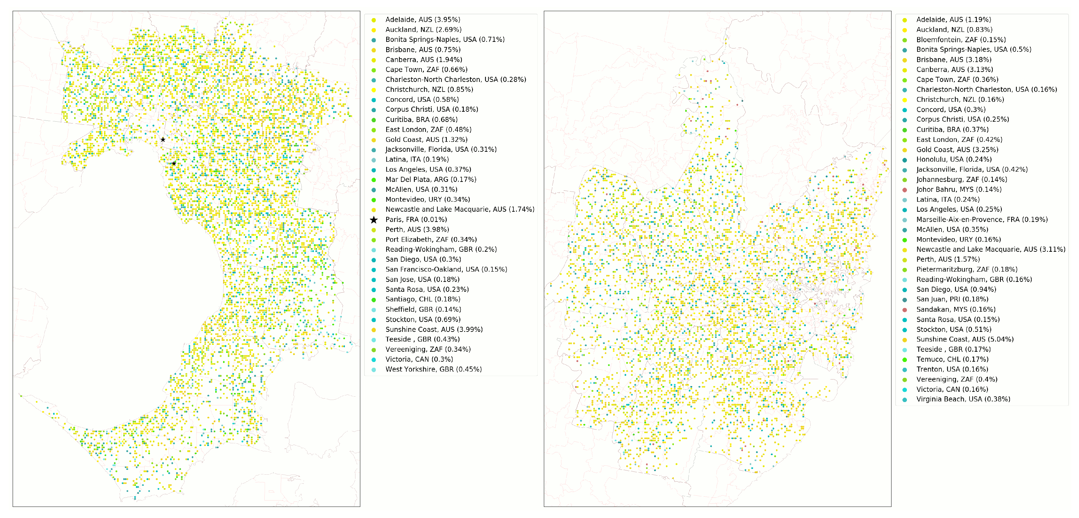
The GSV-BSV (street view) neural network predictions (Table 2c) show strong similarities between Melbourne and Sydney. In the Melbourne evaluation, just under 18% (seven of the top nine picks) are other Australian cities, while Sydney matched other Australian cities in 20.5% of the evaluation locations (and were seven of the top seven picks) and spread somewhat evenly through these other cities. In addition, 15 of the top 20 predicted cities were shared between Melbourne and Sydney.

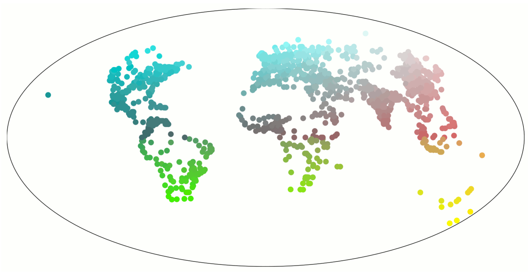
To explore the identified differences, cities predicted for an evaluation location were plotted on maps of Melbourne and Sydney, with the colour scheme for the plots determined by the latitude and longitude of the predicted city. This colour scheme is shown in Figure 2. As such, in the following figures, predicted cities in Australia will show up in shades of yellow, the rest of the Southern Hemisphere in greens, Asia in reds, North America and Europe in blues, and the Middle East in blue-greys.

3.2. Melbourne Evaluation

Figure 3 shows the top predicted cities (>0.1%) plotted against the Melbourne evaluation locations for the GM neural network. Further, “Paris-like” evaluation locations within Melbourne and Sydney are highlighted with black stars (22 in total, but five with probabilities greater than 50%). As can be seen, Australian cities (in yellow) show strong groupings in the inner and outer suburbs while the central business district (CBD) region shows no single strong grouping of regions or specific cities. In Melbourne’s far outer suburbs and rural areas, a wide mix of North and South American, South African, European, and Mid-Eastern cities (in greens blues and greys) with small localised clusters of each can be seen. In the CBD, a few locations are predicted as Paris, and are mostly associated with Docklands or parklands.

Figure 4 shows the top predicted cities (>0.1%) plotted against the Melbourne evaluation locations for the GS neural network with “Paris-like” locations again highlighted with a black star (one location, but 0 locations above 50% probability). Other Australian cities (yellows) show a strong grouping in the inner and outer suburbs, while the CBD region shows no single strong grouping of regions or specific cities but with a range of predictions including Miami, United States (blues) and Mendoza, Argentina (greens). In Melbourne’s far outer suburbs and rural areas, a wide mix is seen of North and South American (USA, Brazil, and Argentina), South African, European (Italy and Spain), and Mid-Eastern (Iran and Turkey) cities with small localised clusters of each. Only a single prediction of Paris, France was made by the GS neural network for any evaluation location in Melbourne (but not above a 50% probability).

Figure 5 shows the top predicted cities (>0.1%) plotted against the Melbourne evaluation locations for the GSV-BSV neural network. "Paris-like" locations are predicted in 13 locations (but only two with a probability over 50%). The overall predictions are dominated by other Australian cities (yellows) scattered widely throughout the entire greater Melbourne area. The remaining evaluation locations show no strong groupings of any predicted countries or cities. Common predictions include cities from South Africa (greens), New Zealand (yellows), and the United States and European countries (blues). The CBD again shows a wide scattering of predictions with no dominant single city or country.

3.3. Sydney Evaluation

Figure 3 shows the top predicted cities (>0.1%) plotted against the Sydney evaluation locations for the GM neural network. “Paris-like” areas are predicted in 54 locations (but only 15 above 50% probability). Alternative Australian cities (yellows) appear in the western and southeastern suburbs, while Mid-Eastern cities (greys) tend to appear in northern and southern suburbs. The CBD and central parts of the city show less single-city or regional groupings but with stronger highly localised clusters of each. Some cities commonly represented in the CBD include waterfront cities such as Hong Kong, London, Toulon, and Kaohsiung.

Figure 4 shows the top predicted cities (>0.1%) plotted against the Sydney evaluation locations for the GS neural network. The overall predictions are dominated by cities in Brazil and other South American locations (greens) in the north, west, and central regions, and Ukraine (blues) in the south. Other Australian cities are only predicted in a few locations around the city. In the CBD, predictions continue to be dominated by Brazilian cities with some more scattered predictions of cities from Japan, Haiti, and Mexico. No predictions of Paris, France were made by the GS neural network for any evaluation location in Sydney.

Figure 5 shows the top predicted cities (>0.1%), plotted against the Sydney evaluation locations for the GSV-BSV neural network. Six “Paris-like” locations were predicted (but none with probabilities greater than 50%). The results are very similar to the Melbourne evaluation. Again, the overall predictions are dominated by other Australian cities scattered widely throughout the entire greater Sydney area. The remaining predicted results show no strong groupings of any predicted countries or cities but some of the common predictions include cities from the United States, New Zealand, South Africa, and a number of European countries. The CBD shows a similar scattering of predictions with no single city or country dominating. A summary of the predicted “Paris-like” locations across all three neural networks for each city is presented in

Table 3. How much are Melbourne and Sydney like Paris? The table shows neural network results, both unfiltered and filtered (where predictions with probabilities less than 50% are removed).

	Melbourne		Sydney
Neural Network	Matches	% Matching	Matches	% Matching
GM	22	0.1	54	0.22
GM (filtered < 50%)	5	0.02	15	0.06
GS	1	0.00004	0	0
GS (filtered < 50%)	0	0	0	0
GSV-BSV	13	0.06	6	0.04
GSV-BSV (filtered < 50%)	2	0.01	0	0

.

3.4. What Cities Are Similar to Paris?

Utilising the confusion each neural network recorded in correctly identifying each city, using an approach from Thompson et al. [10], we identified which other cities shared similar features with Paris. A confusion matrix [57] was generated for each neural network and cities were ranked by the frequency that each was incorrectly identified as Paris.

The GM neural network, which achieved an accuracy of 73.2%, most commonly misidentified the following cities as Paris, ranked in order of decreasing frequency: London, GB, Berlin, DE, New York, US, Rome, IT, Los Angeles, US, Tokyo, JP, Zurich, CH, Istanbul, TR, Brasília, BR, and Munich, DE.

The GSV-BSV neural network, which achieved an accuracy of 43.1%, most commonly misidentified the following cities as Paris, ranked in order of decreasing frequency: Toulouse, Lyon, Rouen, Saint-tienne, Strasbourg, Bordeaux, Lille, Montpellier, Douai-Lens, Grenoble, Nantes, Valenciennes, Tours, and Toulon (all in France).

The GS neural network, which achieved a final trained accuracy of 99.4%, confused no other cities with Paris. In order to add some confusion, we rolled back to an earlier training iteration. At epoch 50, the neural network achieved an accuracy of 74.5% (top five: 92.7%) and most commonly misidentified the following cities as Paris, ranked in order of decreasing frequency: New York, US, Vancouver, CA, Karlsruhe, DE, Brisbane, AU, Colorado Springs, US, Genova, IT, Lisbon, PT, and Montpellier, FR.

4. Discussion

In this study, we used the question of “Is there a ‘Paris-end’ of Melbourne or Sydney” as a means of answering a broader, more important question of how the use of three different sources of available imagery might be used to identify urban typologies. There are a number of different ways to look at the large number of results resulting from the three different large datasets. Figure 3, Figure 4 and Figure 5 contain an implicit assumption embedded in the colour scheme that geographically close locations are similar. While this is true for the cities that are like Paris (in Section 3.4) for the GSV-BSV neural network, it is not the case for the other two neural networks. Conversely, the figures show that Melbourne and Sydney (for the GM and to a lesser extent the GS neural network) show localised clustering of locations that are similar to other (geographically similar) cities while the GSV-BSV network shows little of this localised clustering across Melbourne and Sydney.

In looking at the few locations that are deemed to be “Paris-like”, there are a number of common characteristics that stand out. A gallery of all of the images for Melbourne and Sydney that the GM neural network found were similar to Paris are presented in Figure 6 and Figure 7. There are a number of common elements in these images. Many show large parklands (in green) embedded in the cities. Orange lines of public transport (rail and tram) are also prominent as well as large water bodies (in blue). Large arterial and trunk roads run near smaller (often curving) local roads; however these local roads tend to still be larger and do not reach the small intricate layouts of many Asian cities. In addition, among the cities misidentified as Paris by the neural networks, large Western European and US cities, including London, Berlin, New York, and Rome, also feature large numbers of these elements.

The GM neural network makes predictions based on mapping imagery, capturing characteristics such as the mix and detail of public transport, green space, water bodies, and the road network structure. This includes whether the roads are grid-like, the mix of arterial vs. neighbourhood roads, and their integration with the rest of the urban form. Seven Australian cities were included in the training data (Perth, Brisbane, Sunshine Coast, Gold Coast, Newcastle and Lake Macquarie, Canberra, and Adelaide) and likely share many common planning and design standards with Sydney and Melbourne, influencing the neural network’s predictions.

Using the GS neural network, none of the evaluated locations for Sydney and only one location for Melbourne were predicted to be "Paris-like". From an overhead remote sensing point of view, there is therefore nothing about either Melbourne or Sydney that shares similar visual characteristics with Paris, or at least there are many other cities that are more similar to Paris than Melbourne and Sydney. The GS network is more strongly influenced by larger natural and topographical features than the GM network. Outside of the immediate city centres, both Melbourne and Sydney are highly vegetated, with large percentages of the built-form concealed under tree canopies and having to conform to topography. The colours of the vegetation and soils as well as how the urban form is mixed into the canopies, hillsides, waterways and oceans are highly influential. Melbourne is built around a bay and around a north–south spine of hills, while Sydney is built around the open ocean and ocean waterways as well as hilly terrain throughout the metro area. Some potential limitations in the dataset can be seen in Figure 4. A strong north–south gradient through the plot of the Melbourne predictions suggests that the neural network detected some artefacts of the satellite imagery gathering process, such as different acquisition times of the imagery, that were not apparent to human observation. The satellite imagery also shows some disadvantages in discovering typologies through a confusion matrix approach. The final trained neural network was too accurate. Finding similarities requires some level of confusion; thus in order to find cities similar to Paris, the neural network had to be rolled back to an earlier, less accurate iteration.

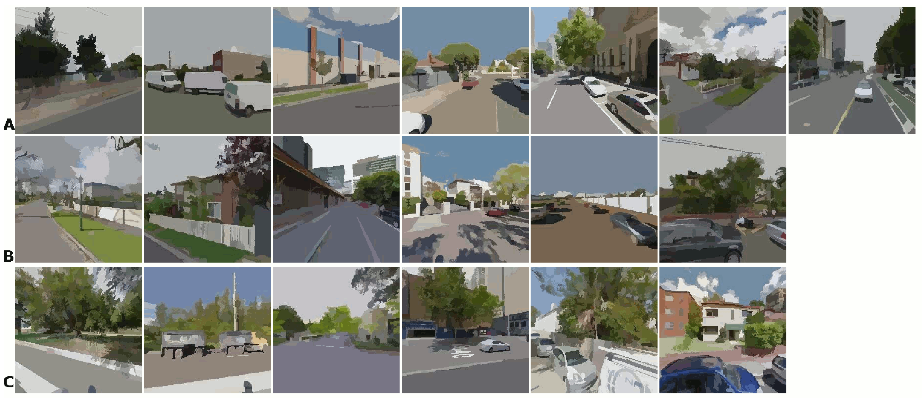
Finally, as the GSV-BSV neural network only picked Paris (at over a 50% probability) for 0.01% of the evaluated locations for Melbourne and 0% for Sydney. We can be confident that from a visual street-level view, there is almost nothing about either Melbourne or Sydney that is visually similar to Paris using this type of imagery. Of the images for Melbourne, only two (out of 13) were picked with a probability of over 50% (and none out of six for Sydney). With the GSV-BSV network (galleries of “Paris-like” images for Melbourne and Sydney are shown in Figure 8), smaller details of the cities will influence predictions. At this level of imagery, many of the natural features influential in the GS network (e.g., types and colours of vegetation or soil) will be important, but smaller details will also weigh in, such as building architecture, the width (or absence) of nature strips or sidewalks, and an overall density of streetscape features. Other influential characteristics are features that are in the urban areas but are not part of the permanent built form. For example, white vans feature in a number of images in the galleries of Paris-like predictions. At this level of imagery, the neural network will be potentially influenced as much by how the urban form is being used (especially how it is used at the time the images are captured) as the form itself. This shows the importance of taking steps in some circumstances to construct abstract features from the source images (e.g., road networks and green space for GM or image segmentation for GSV-BSV). Even with these measures, some caution should be taken with this type of imagery. The rather low accuracy rate for GSV-BSV (43.1%, top five: 69.8%) indicates that larger training datasets or perhaps fewer classification classes are needed with this type of complex imagery. When the low accuracy is analysed with a confusion matrix, it is found that the other cities that are confused for Paris are most often other French cities. This suggests that this group of similar French cities might form a better basis for a typology classification than the single city Paris. It also suggests that care is needed to balance the mix of accuracy and confusion. While the highly accurate GS neural network was unable to misidentify cities, the GSV-BSV neural network was better suited to find similarities through confusion.

Using the GM neural network approach, urban form can be evaluated. Map characteristics that are influential in grouping cities with a particular typology include extents and types of public transportation, urban green space, road network structure, water body inclusion and integration, amounts of informal unplanned open space, and density and topology influences on city structure. Some of the features included in the GM imagery that made cities “Paris-like” were a higher density of trains and trams, large broad sections of urban green space, and an integration of urban green space and waterways. Of course, while Paris was selected as the comparison city of choice, the technique makes it possible to typify the characteristics of any global city where similar imagery is available.

In Thompson et al. [10] and Nice et al. [33], highly abstract map imagery was found to lend itself to finding similarities between cities and identifying clusters of similar cities or inner-city neighbourhoods, as well as associations due to different urban typologies with outcomes to public health, such as road trauma or pollution levels. This type of imagery fits in well with the first urban typology scale of Argan and Rykwert [18], the arrangements of streets and buildings in urban areas.

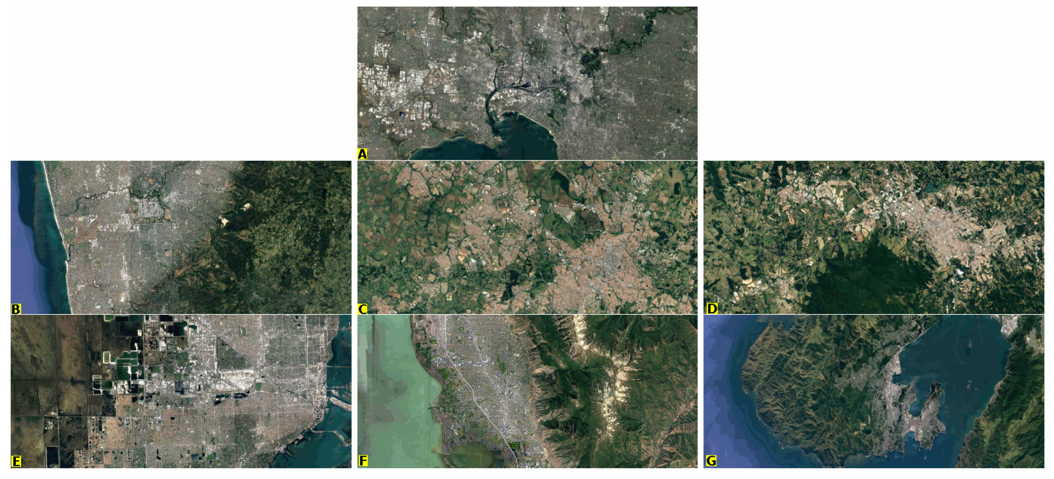
Using satellite imagery, natural features and the colour characteristics of rooftops, streets, soil, and vegetation feature predominantly in classifying locations within a particular typology. In Figure 9A, satellite imagery of Melbourne shows a number of colour and terrain similarities with the GS top six predictions, namely Adelaide, Australia; Campinas, Brazil; Jundiaí, Brazil; Miami, USA; Provo, USA; and Wellington, NZ (all shown in Figure 9). This perhaps shows that natural characteristics are more influential to what the GS neural network considers to make cities similar than the characteristics of built urban form highlighted by the GM model.

The satellite imagery fits less well into a particular Argan and Rykwert [18] scale. The area covered by the imagery is identical to the map imagery (400 × 400 m), capturing the road and building structure of each area. However, the imagery also contains information suitable for generating typologies based on the constructed elements scale as well as the decorative elements of the area (from a vertical vantage point). To create stronger typologies, additional steps will likely be needed to push the typologies towards one or the other scales. Analysis of areas smaller than 400 × 400 m can allow details more relevant to the building or decorative scales to be emphasized. However, this might require higher resolution imagery than the 15 m resolution imagery provided by Google to ensure sufficient detail. To better capture the street and building structure, pre-processing could be applied (edge detection, mean shifts, or other computer vision techniques) to force a stronger emphasis on the urban structure rather than the details. Further additional work could be performed, such as deconstructing and reconstructing imagery, removing features (such as automotive traffic, leaving only structures), and, for targeted outcomes (such as health and social capital), using generative adversarial networks [58], enabling comparative hypothetical typology scenarios.

Finally, in examining the results from the GSV-BSV neural network, this micro-scaled level of imagery would arguably capture the visual geography of the streetscape; what most people would say captures that which “makes Paris looks like Paris”. This imagery fits well into the detailed/decorative Argan and Rykwert [18] scale. However, as Doersch et al. [32] found in trying to answer the same question, overall this answer is not based on a small number of famous iconic landmarks (e.g., the Eiffel Tower or the Louvre), but on an array of widespread, smaller features. These features include elements such as cast-iron railings on balconies, grid-like balcony arrangements, distinctive street signs, streetlamps on pedestals, window balustrades, Parisian doorways, six-story Haussmann apartment buildings, and vegetation differences [59]. Of all these micro-scaled visual elements, neither Melbourne nor Sydney contain enough to truly have a “Paris-like” district.

Additionally, as found in this study, the characteristics that make up a city on a visual street view level are a complex mix. This not only includes bigger structural details, such as buildings, roads, cars, vegetation, and street furniture, but also smaller less-apparent details, such as colours, weather conditions, road markings, and thousands of other small details. The complexity of this imagery and the subsequent low accuracy of the neural networks in identifying individual cities using it indicates that further steps are needed to use this type of imagery reliably. These steps can include training using a smaller pool of cities and using a smaller set of classifications to allow focus on more subtle differences. In addition, more aggressive preprocessing (beyond the mean shift segmentation preprocessing we used) might be needed to further reduce the complexity of the imagery, using techniques such as foreground/background subtraction or inpainting to remove detail from the images less relevant to the intended typology goal.

This project’s intended goal was to demonstrate the ability of this new methodology to compare and cluster entire cities based on the summation of smaller localised details of urban form. As such, the imagery sampling collected imagery from the entire wider city and was not restricted to the perhaps more distinctive city centres. The results reflect that focus and show one of the strengths of this technique, allowing comparisons between entire cities as a whole and allowing linkages to datasets (health, transportation, etc.) that exist at city levels. However, this also demonstrates that appropriate consideration needs to be paid to the goals of a particular analysis, and that, for example, identifying distinctive city centres in other cities might require adjustment of the sampling radius for the training data.

Future work is planned to vary these techniques and further evolve the insights gained. Inner-city comparisons will sample imagery from within cities and help answer questions such as does (wider) Paris look like (the iconic districts of) Paris? Conversely, removing all the other Australian cities from the training data will allow comparisons to be made on a strictly international basis. Cross-comparisons can also assess similarities between individual cities under different contexts (e.g., varying which other cities are included in the pool of comparison cities). Further work, based on Thompson et al. [10], will use a confusion matrix/graph-based approach to find clusters of urban design types, based on their levels of similarity between the cities, and apply these typologies to outcomes related to public health (such as road trauma, pollution levels, and likeliness to engage in active transport.).

5. Conclusions

This analysis revealed a number of exciting possibilities for using neural networks to analyse urban form. Using this method, any city in the world can now find other cities similar to itself with easily obtained and globally consistent imagery. This methodology can be used to look at many different aspects of cities and understand what elements of their urban design leads them to work in different ways and allow accounting for local context when applying successful policies from other cities.

6. Data Availability

Datasets and trained neural networks are available from the corresponding author upon request.

References

1. Giles-Corti, B.; Vernez-Moudon, A.; Reis, R.; Turrell, G.; Dannenberg, A.L.; Badland, H.; Foster, S.; Lowe, M.; Sallis, J.F.; Stevenson, M.; et al. Urban design, transport, and health 1 City planning and population health: A global challenge. Lancet 2016, 6736, 1–13. [Google Scholar] [CrossRef]
2. Kleinert, S.; Horton, R. Urban design: An important future force for health and wellbeing. Lancet 2016, 6736, 1–11. [Google Scholar] [CrossRef]
3. Goenka, S.; Andersen, L.B. Urban design and transport to promote healthy lives. Lancet 2016, 6736, 8–10. [Google Scholar] [CrossRef]
4. Norman, J.; MacLean, H.L.; Kennedy, C.A. Comparing High and Low Residential Density: Life-Cycle Analysis of Energy Use and Greenhouse Gas Emissions. J. Urban Plan. Dev. 2006, 132, 10–21. [Google Scholar] [CrossRef]
5. Daley, M.; Rissel, C. Perspectives and images of cycling as a barrier or facilitator of cycling. Transp. Policy 2011, 18, 211–216. [Google Scholar] [CrossRef]
6. Zapata-Diomedi, B.; Knibbs, L.D.; Ware, R.S.; Heesch, K.C.; Tainio, M.; Woodcock, J.; Veerman, J.L. A shift from motorised travel to active transport: What are the potential health gains for an Australian city? PLoS ONE 2017, 12, 1–21. [Google Scholar] [CrossRef] [Green Version]
7. Heesch, K.C.; Giles-Corti, B.; Turrell, G. Cycling for transport and recreation: Associations with socio-economic position, environmental perceptions, and psychological disposition. Prev. Med. 2014, 63, 29–35. [Google Scholar] [CrossRef] [Green Version]
8. Cepeda, M.; Schoufour, J.; Freak-poli, R.; Koolhaas, C.M.; Dhana, K.; Bramer, W.M.; Franco, O.H. Levels of ambient air pollution according to mode of transport: A systematic review. Lancet Public Health 2016, 2, e23–e34. [Google Scholar] [CrossRef] [Green Version]
9. Ming Wen, L.; Rissel, C. Inverse associations between cycling to work, public transport, and overweight and obesity: Findings from a population based study in Australia. Prev. Med. 2008, 46, 29–32. [Google Scholar] [CrossRef] [Green Version]
10. Thompson, J.; Stevenson, M.; Wijnands, J.S.; Nice, K.A.; Aschwanden, G.D.P.A.; Silver, J.; Nieuwenhuijsen, M.; Rayner, P.; Schofield, R.; Hariharan, R.; et al. A global analysis of urban design types and road transport injury: An image processing study. Lancet Planet. Health 2020, 4, 32–42. [Google Scholar] [CrossRef] [Green Version]
11. Wegener, M.; Gnad, F.; Vannahme, M. The Time Scale of Urban Change. In Advances in Urban Systems Modelling; Hutchinson, B., Batty, M., Eds.; Spiekermann-Wegener: Amsterdam, The Netherlands, 1986; pp. 175–197. [Google Scholar]
12. Strano, E.; Nicosia, V.; Latora, V.; Porta, S.; Barthélemy, M. Elementary processes governing the evolution of road networks. Sci. Rep. 2012, 2. [Google Scholar] [CrossRef] [Green Version]
13. Mundigo, A.I.; Crouch, D.P. The City Planning Ordinances of the Laws of the Indies Revisited. Part I: Their Philosophy and Implications. Town Plan. Rev. 1977, 48, 247–268. [Google Scholar] [CrossRef]
14. Bandini, M. Typology As A Form Of Convention. AA Files 1984, 6, 73–82. [Google Scholar]
15. Rossi, A. The Architecture of the City; The MIT Press: Cambridge, MA, USA, 1982; p. 201. [Google Scholar]
16. Krier, R. Urban Space; Academy Editions: London, UK, 1979; p. 173. [Google Scholar]
17. Crouch, D.P.; Mundigo, A.I. The City Planning Ordinances of the Laws of the Indies Revisited. Part II: Three American Cities. Town Plan. Rev. 1977, 48, 397–418. [Google Scholar] [CrossRef]
18. Argan, C.G.; Rykwert, J. On the Typology of Architecture. Archit. Des. 1963, 33, 564–565. [Google Scholar]
19. Harris, C.D. A Functional Classification of Cities in the United States. Geogr. Rev. 1943, 33, 86–99. [Google Scholar] [CrossRef]
20. Nelson, H.J. A Service Classification of American Cities. Econ. Geogr. 1955, 31, 189–210. [Google Scholar]
21. Bruce, G.D.; Witt, R.E. Developing Empirically Derived City Typologies: An Application of Cluster Analysis. Sociol. Q. 1971, 12, 238–246. [Google Scholar] [CrossRef]
22. Hillier, B. Space Is the Machine; Cambridge University Press: Cambridge, UK, 1996. [Google Scholar] [CrossRef]
23. Zhang, Q.; Seto, K.C. Can night-time light data identify typologies of urbanization? A global assessment of successes and failures. Remote Sens. 2013, 5, 3476–3494. [Google Scholar] [CrossRef] [Green Version]
24. Hermosilla, T.; Palomar-Vázquez, J.; Balaguer-Beser, Á.; Balsa-Barreiro, J.; Ruiz, L.A. Using street based metrics to characterize urban typologies. Comput. Environ. Urban Syst. 2014, 44, 68–79. [Google Scholar] [CrossRef] [Green Version]
25. Stewart, I.D.; Oke, T.R. Local Climate Zones for Urban Temperature Studies. Bull. Am. Meteorol. Soc. 2012, 93, 1879–1900. [Google Scholar] [CrossRef]
26. Stewart, I.D.; Oke, T.R.; Krayenhoff, E.S. Evaluation of the ‘local climate zone’ scheme using temperature observations and model simulations. Int. J. Climatol. 2014, 34, 1062–1080. [Google Scholar] [CrossRef]
27. Liu, L.; Zhou, B.; Zhao, J.; Ryan, B.D. C-IMAGE: City cognitive mapping through geo-tagged photos. GeoJournal 2016, 81, 817–861. [Google Scholar] [CrossRef] [Green Version]
28. Zhou, B.; Liu, L.; Oliva, A.; Torralba, A. Recognizing city identity via attribute analysis of geo-tagged images. In Computer Vision—ECCV 2014. ECCV 2014. Lecture Notes in Computer Science; Fleet, D., Pajdla, T., Schiele, B., Tuytelaars, T., Eds.; Springer: Cham, Switzerland, 2014; Volume 8691, pp. 519–534. [Google Scholar] [CrossRef] [Green Version]
29. Dubey, A.; Naik, N.; Parikh, D.; Raskar, R.; Hidalgo, C.A. Deep learning the city: Quantifying urban perception at a global scale. In Computer Vision—ECCV 2016; Lecture Notes in Computer Science (Including Subseries Lecture Notes in Artificial Intelligence and Lecture Notes in Bioinformatics); Springer: Cham, Switzerland, 2016; pp. 196–212. [Google Scholar] [CrossRef] [Green Version]
30. Naik, N.; Philipoom, J.; Raskar, R.; Hidalgo, C. Streetscore—Predicting the Perceived Safety of One Million Streetscapes. In Proceedings of the 2014 IEEE Conference on Computer Vision and Pattern Recognition Workshops, Columbus, OH, USA, 23–28 June 2014; pp. 793–799. [Google Scholar] [CrossRef] [Green Version]
31. Salesses, P.; Schechtner, K.; Hidalgo, C.A. The Collaborative Image of The City: Mapping the Inequality of Urban Perception. PLoS ONE 2013, 8. [Google Scholar] [CrossRef] [Green Version]
32. Doersch, C.; Singh, S.; Gupta, A.; Sivic, J.; Efros, A. What Makes Paris Look like Paris? ACM Trans. Graph. Assoc. Comput. Mach. 2012, 31, HAL Id:hal-01053876. [Google Scholar] [CrossRef]
33. Nice, K.; Aschwanden, G.; Wijnands, J.S.; Thompson, J.; Zhao, H.; Stevenson, M. The Nature of Human Settlement: Building an understanding of high performance city design. arxiv 2019, arXiv:1910.03219. [Google Scholar]
34. Anholt, S. The Anholt-GMI City Brands Index: How the world sees the world’s cities. Place Brand. 2006, 2, 18–31. [Google Scholar] [CrossRef]
35. Williams, R. Tower plans cast shadow over Collins Street’s Paris end. The Age, 10 May 2010. [Google Scholar]
36. Wilden, N. ’France-Soir: A bite of Paris on the Yarra’. The Australian, 2 December 2013. [Google Scholar]
37. Bishop, C.M. Neural Networks for Pattern Recognition; Clarendon Press: Oxford, UK, 1995; p. 482. [Google Scholar]
38. Samarasinghe, S. Neural Networks for Applied Sciences and Engineering: From Fundamentals to Complex Pattern Recognition; CRC Press: Boca Raton, FL, USA, 2016; p. 570. [Google Scholar]
39. Graupe, D. Advanced Series in Circuits and Systems: Volume 7 Principles of Artificial Neural Networks, 3rd ed.; University of Illinois: Chicago, IL, USA, 2013. [Google Scholar]
40. Schmidhuber, J. Deep Learning in neural networks: An overview. Neural Netw. 2015, 61, 85–117. [Google Scholar] [CrossRef] [Green Version]
41. Szegedy, C.; Liu, W.; Jia, Y.; Sermanet, P.; Reed, S.; Anguelov, D.; Erhan, D.; Vanhoucke, V.; Rabinovich, A. Going deeper with convolutions. In Proceedings of the IEEE Computer Society Conference on Computer Vision and Pattern Recognition, Boston, MA, USA, 7–12 June 2015; pp. 1–9. [Google Scholar] [CrossRef] [Green Version]
42. Ioffe, S.; Szegedy, C. Batch Normalization: Accelerating Deep Network Training by Reducing Internal Covariate Shift. In Proceedings of the 32nd International Conference on Machine Learning, Lille, France, 6–11 July 2015. [Google Scholar] [CrossRef]
43. United Nations. World Urbanization Prospects; The 2014 Revision, CD-ROM Edition; Department of Economic and Social Affairs, Population Division: New York, NY, USA, 2014. [Google Scholar]
44. Barthelemy, M. The Structure and Dynamics of Cities: Urban Data Analysis and Theoretical Modeling; Cambridge University Press: Cambridge, UK, 2016; p. 278. [Google Scholar] [CrossRef] [Green Version]
45. Day, J.; Chen, Y.; Ellis, P.; Roberts, M. A Free, Open-Source Tool for Identifying Urban Agglomerations using Point Data. Spat. Econ. Anal. 2016, 11, 67–91. [Google Scholar] [CrossRef]
46. Day, J.; Chen, Y.; Ellis, P.; Roberts, M. A free, open-source tool for identifying urban agglomerations using polygon data. Environ. Syst. Decis. 2017, 37, 68–87. [Google Scholar] [CrossRef]
47. Quistberg, D.A.; Roux, A.V.D.; Bilal, U.; Moore, K.; Ortigoza, A.; Rodriguez, D.A.; Sarmiento, O.L.; Frenz, P.; Friche, A.A.; Caiaffa, W.T.; et al. Building a Data Platform for Cross-Country Urban Health Studies: The SALURBAL Study. J. Urban Health 2019, 96, 311–337. [Google Scholar] [CrossRef] [PubMed] [Green Version]
48. Arribas-Bel, D.; Garcia-Lopez, M.A.; Viladecans-Marsal, E. Building(s and) cities: Delineating urban areas with a machine learning algorithm. J. Urban Econ. 2019. [Google Scholar] [CrossRef] [Green Version]
49. Dijkstra, L.; Poelman, H.; Veneri, P. The EU-OECD Definition of a Functional Urban Area; OECD Regional Development Working Papers; OECD: Paris, France, 2019. [Google Scholar] [CrossRef]
50. Sinnott, R. Virtues of the Haversine. Sky Telesc. 1984, 68, 159. [Google Scholar]
51. Google Maps. Google Static Maps API. 2017. Available online: https://developers.google.com/maps/documentation/static-maps (accessed on 15 June 2017).
52. Google Maps. Google Street View API. 2017. Available online: https://developers.google.com/maps/documentation/streetview/ (accessed on 15 June 2017).
53. Google. Only Clear Skies on Google Maps and Earth. 2013. Available online: https://maps.googleblog.com/2013/06/only-clear-skies-on-google-maps-and.html (accessed on 20 April 2020).
54. Baidu. Baidu Street View API. 2017. Available online: http://api.map.baidu.com/ (accessed on 15 June 2017).
55. Pymeanshift. Python Module for Mean Shift Image Segmentation. 2017. Available online: https://github.com/fjean/pymeanshift (accessed on 15 June 2017).
56. Yu, D.; Eversole, A.; Seltzer, M.L.; Yao, K.; Huang, Z.; Guenter, B.; Kuchaiev, O.; Zhang, Y.; Seide, F.; Wang, H.; et al. An Introduction to Computational Networks and the Computational Network Toolkit. Microsoft Technical Report MSR-TR-2014–112; Technical Report; Microsoft: Redmond, WA, USA, 2015. [Google Scholar]
57. Kohavi, R.; Provost, F. Glossary of Terms. Mach. Learn. 1998, 30, 271–274. [Google Scholar]
58. Wijnands, J.S.; Nice, K.A.; Thompson, J.; Zhao, H.; Stevenson, M. Streetscape augmentation using generative adversarial networks: Insights related to health and wellbeing. Sustain. Cities Soc. 2019. [Google Scholar] [CrossRef] [Green Version]
59. Li, X.; Zhang, C.; Li, W.; Ricard, R.; Meng, Q.; Zhang, W. Assessing street-level urban greenery using Google Street View and a modified green view index. Urban For. Urban Green. 2015, 14, 675–685. [Google Scholar] [CrossRef]
Figure 1. Sample neural network training images for (a) GM (from Paris, France [51]), (b) GS (from Adelaide, Australia [51]), and (c) for GSV-BSV after mean shift pre-processing (from Sydney, Australia [52]).
Urbansci 04 00027 g001
Figure 2. Latitude–longitude-based colour scheme for plotting neural network predictions of cities similar to Melbourne and Sydney.
Urbansci 04 00027 g002
Figure 3. Predicted similar cities using the GM neural network (filtering out probabilities lower than 50%). Top predicted cities plotted (using Figure 2 colour scheme) for Melbourne evaluation locations (left) and Sydney (right). Predicted Paris locations marked with black stars.
Urbansci 04 00027 g003
Figure 4. Predicted similar cities using the GS neural network (filtering out probabilities lower than 50%). Top predicted cities plotted (using Figure 2 colour scheme) for Melbourne evaluation locations (left) and Sydney (right). Predicted Paris locations marked with black stars.
Urbansci 04 00027 g004
Figure 5. Predicted similar cities using the GSV-BSV neural network (filtering out probabilities lower than 50%). Top predicted cities plotted (using Figure 2 colour scheme) for Melbourne evaluation locations (left) and Sydney (right). Predicted Paris locations marked with black stars.
Urbansci 04 00027 g005
Figure 6. Gallery of “Paris-like” locations in Melbourne using the GM neural network.
Urbansci 04 00027 g006
Figure 7. Gallery of “Paris-like” locations in Sydney using the GM neural network.
Urbansci 04 00027 g007
Figure 8. Gallery of “Paris-like” locations in Melbourne (A and B) and Sydney (C) using the GSV-BSV neural network.
Urbansci 04 00027 g008
Figure 9. Satellite imagery of Melbourne, Australia (A), Adelaide, Australia (B), Campinas, Brazil (C), Jundiaí, Brazil (D), Miami, USA (E), Provo, USA (F), and Wellington, NZ (G) [51]. Note that the training imagery for the GM network was captured at a 400 × 400 m resolution (see Figure 1), not at the city-wide scale depicted here.
Urbansci 04 00027 g009