Article

An Investigation of Links between Environmentally Responsible Behaviors and Built and Natural Features of Landscape in Central New Jersey

by
Daniel G. Clark
1,* and
Rebecca C. Jordan
2
1
Graduate Program in Ecology and Evolution, Rutgers, the State University of New Jersey, New Brunswick, NJ 08901, USA
2
Community Sustainability, College of Agriculture and Natural Resources, Michigan State University, East Lansing, MI 48824, USA
*
Author to whom correspondence should be addressed.
Urban Sci. 2018, 2(4), 114; https://doi.org/10.3390/urbansci2040114
Submission received: 20 August 2018 / Revised: 3 November 2018 / Accepted: 22 November 2018 / Published: 29 November 2018

Abstract

:
Responses from Central New Jersey residents (n = 290) to nine survey items about pro-environmental behaviors were analyzed for their connection to survey respondents’ local built and natural landscape characteristics. These nine survey items were of interest due to their clustering in three groups in earlier dimension reduction analysis. Nine logistic regression models (one for each of these items) were built using a suite of built and natural features of landscape at the municipal level—including land use, population density, and access to parks. The logistic regression models using the landscape variables failed to provide effective explanations of engagement in pro-environmental behavior. In total, only ten landscape feature variables—out of a possible thirty-eight -were used in any of the most effective models. The logistic regression model of proper appliance disposal performed best and could correctly classify responses of whether respondents had disposed of an appliance correctly 84% of the time. The rest of the models were of little use. This suggests that there may not be a connection between these built and natural landscape features and these behaviors, or that the study did not look at location at a level that was granular enough to detect any patterns.

1. Introduction

There are a wide range of threats facing humanity that endanger our continued ability for communities to thrive—most of which can be conclusively linked to anthropogenic climate change [1,2]. In the face of this, it is necessary to come up with effective solutions for lowering consumption of resources, and increasing conservation and preservation behaviors. There are many possible ways of framing these types of behavior—as pro-environmental behaviors [3,4,5,6], environmentally responsible behaviors [7,8], and environmentally significant behaviors [9,10]. While there are some distinctions among these, fundamentally, they are talking about some set of actions and behaviors undertaken by humans that benefit some conception of the environment in some way (or, at the very least, reduce harm to the environment); some of these definitions include that behaviors be explicitly intentional in this regard, others are more outcome focused, regardless of intentionality. This research was undertaken with the express purpose of measuring the extent to which nine of these behaviors could be linked to built and natural features of landscape. Knowledge of links between features of landscape and behaviors are useful in generating tools that policy-makers and managers can use to manage landscapes to encourage specific behaviors and to achieve certain behaviors as outcomes.
Throughout this paper we will be using the terms Environmentally Responsible Behaviors (ERBs). Our framing of this term recognizes the wide breadth of work on the subject [4,5,9,11,12,13,14,15]. However, we rely heavily on an outcome-driven conception of behaviors, based on Stern’s framework of “the extent to which it changes the availability of materials or energy from the environment or alters the structures or dynamics of ecosystems or the biosphere itself” [10].
Research in the field of environmental literacy, engagement, and knowledge has established that there is not necessarily a clear link between environmental literacy and pro-environmental behaviors [16,17,18,19,20,21]; leading us to ask what drives pro-environmental behavior. Many studies have linked specific types of environmental knowledge and behavior to a series of intrinsic and external factors [18,20,22,23,24,25]. Clearly, a lack of pro-environmental behavior does not singularly result from a lack of knowledge [26]. Therefore, there must be other factors influencing these behaviors.
Exposure to nature or green spaces has been linked to environmental engagement [17,18,20,22,23,24]. Persons living in more forested areas were thought to be more likely to spend more time outside [27,28,29]. Based on this, we hypothesized that engagement in ERBs could be linked to certain built and natural features of the landscape. Research to date has demonstrated that some portions of connectedness to nature are related to experiences outside [3,13,22,30,31,32]. Furthermore, certain behaviors—especially related to health and activity—have been conclusively linked to features of the built and natural landscape [3,5,14,33,34,35,36,37].
Based on research to date in this field, we hypothesized that specific features of the built and natural landscape could be conclusively linked to individual ERBs in individuals. Due to work linking exposure to greenery with environmental concern [33,34,38,39,40], we hypothesized that exposure to increased greenery within the landscape will increase awareness or concern about the environment. In turn, this would then lead to higher frequencies of engagement in ERBs. Central New Jersey was chosen as the study area because it presents a landscape with major changes over short distances—there are landscapes dominated by forest, agriculture, and commercial/industrial infrastructure in a single county [41]. The municipalities of New Jersey also present large differences in a small geographic area across income, education, ethnicity, and race, also within a single county [42]. Furthermore, the authors have performed some prior survey and interview work in this area that was useful in steering the survey instrument [16,43,44,45,46].
We hypothesized that landscape with greater amounts of forest cover, parks and recreation opportunities, and access to these parks, green spaces, and recreation areas would increase participation in environmentally responsible behaviors (ERBs) among residents. Positive experiences within the outdoors has been demonstrated as an important predictor of engagement with the environment [32,47,48,49]. Therefore, we hypothesized that persons living in areas that were more accessible—either by foot or car—would spend more time outside, and therefore be more likely to care about the environment.
We were not assuming the direction of causality in any relationship between landscape and ERBs, and acknowledge that there are multiple potential feedback loops in this process- people engaged in ERBs may intentionally move to a landscape, landscapes may lead to an increase in ERB engagement, persons engaged in ERBs may actively change a landscape, and there may be feedback loops involving any combination of these phenomena. The complicated origin of ERBs in individuals has been written about elsewhere [10,26,47,48,50,51]. This research was undertaken to seek these connections because the factors of landscape involved can possibly be influenced by management and policy decisions. Once relationships between ERBs and built and natural features of landscape are established, causal connections could be further researched. This way future management decisions could target landscape features that are causal in increasing engagement in ERBs.
One main goal for this study was to provide a tool that could be used by decision-makers, planners, and landscape managers. They could use existing landscape data, plug in various proposed changes they might like to make, and see how these landscape-level changes might influence the behavior(s) of various segments of their population. Therefore, a model that can correctly classify respondents as engaging or not engaging in a behavior at a high rate would be desirable, and one that only provided correct classification at a lower rate would not be particularly useful. In this research, we seek to build a series of logistics binary regression models for nine ERBs that would allow such a tool to be built.

2. Materials and Methods

2.1. Questionnaire

In the summer of 2016, 290 respondents were surveyed on a range of items including demographic information, use of outdoor recreation spaces, and environmentally responsible decision-making behavior. We purchased the sample from Qualtrics, who collected these data via the internet (on computers and mobile devices). Qualtrics is a U.S. based company that bills themselves on their website as performing “experience management”. Among other things, they conduct market research. The authors’ institution has a subscription to Qualtrics, and at the time of this study, both authors were very familiar with use of this platform. Additionally, other similar services were contacted for price quotes and Qualtrics was the platform where the highest number of responses could be gathered for the amount of funds budgeted for this project.
Criteria for inclusion were residence within the study area and being an adult aged eighteen or older. Respondents were also required to respond affirmatively to a consent form based on IRB anonymous consent protocol. All research was carried out in accordance with Rutgers IRB [#E15-678]. Respondents were identified for their location at the level of the municipality. This survey instrument can be found in its entirety in the Supplementary, as can descriptive statistics for survey items.
The final instrument used was developed through several rounds of piloting and testing based on previous work, the scope and aims of this study, and input from pilot respondents. Questions on demographic information were based on the U.S. Census [42]. These items included age, race, ethnicity, income, household makeup, and pets. The items chosen for inclusion on Environmentally Responsible Behaviors (ERBs), were based on six distinct categories: Direct Actions, Community and Civic Behaviors, Political Engagement, Consumer—consumable goods, Consumer non-consumable goods, and Identity—surveying respondents on thirty-eight pro-environmental behavioral items. These items were based on the background discussed above [6,9,15,43,52].
Earlier work with this dataset uncovered three latent sets of ERBs within the survey items. We used generalized canonical correlation analysis to identify three distinctive sets of behavior, each made of three individual behaviors. Behavioral items were grouped into sets together when respondents answered similarly across the behavioral items within a group; they are not behaviors that are similar in terms of the type of behavior or function that they entail. These groups of behaviors could be graphically represented as occupying similar positions in our dimensionality reduction analysis, indicating that respondents answered survey items similarly. Furthermore, these were all highly weighted within that dimensionality reduction indicating that these were areas wherein there were differences among responses that followed some set pattern. Some responses were dropped from analysis due to non-responses. Therefore, our research postulated that there were underlying factors not readily apparent that could be used to explain each group of behaviors. A more detailed description of this work is given in the Supplementary section.
A graphical representation of these clusters is given below in Figure 1. The term CCV refers to the Canonical Correlation Variables. The locations within the space indicate how similar or dissimilar responses were to the survey items. Two very close CCVs would indicate a high level of similarity across two responses. The further a CCV is from the origin, the greater the amount of difference represented throughout the study population. All three clusters included behaviors that were closer to each other on the first canonical correlation variables than to any other behaviors, and had a total distance of fewer than 0.1 units. A list of all behaviors surveyed, and more detailed results of this analysis can be found in the Supplementary section. The specific wording of these items is given below in Table 1.
These behaviors were expected to fall into six a priori groups based on previous work with this population, and similar studies within the field. [15,16,43,44]. These a priori groups were direct actions, community and civic engagement, political engagement, identity, and consumer behavior. Consumer behavior was split into consumer behavior surrounding consumable products such as food and non-consumable products such as appliances. For example, a person who engaged in pro-environmental consumer behavior in their purchasing of consumable products would be expected to report caring about the origin and production methods of their groceries as well as those of hygiene products; a person who engaged in pro-environmental identity behaviors would report that they think of themselves as an environmentalist and also thought about the environmental impacts of their actions. We then hypothesized that these behaviors were linked to differences in land cover and other features of the landscape and built environment, and that respondents who undertook the identified sets of activities lived in physical environments that were alike in a quantifiable way.

2.2. Landscape Information and Data

The landcover data for the study was downloaded from the New Jersey DEP Bureau of GIS, using the 2012 Land Use/Land Cover dataset [41]. These data are classified based on a modified version of the Anderson system. The data for roadway locations in this study came from the New Jersey Department of Transportation [53], incorporated with roadways maps from the DEP [41].
The locations for parks was based on maps generated in the Grant F. Walton Center for Remote Sensing and Spatial Analysis (CRSSA), which maintains maps of this type for New Jersey [54]. The PAD-US database [55] was used to check some locations, however, due to enhanced levels of specificity, ground truthing, and local knowledge of the CRSSA cartographers of this region, conflicts generally were defaulted to the map from CRSSA.
From these data sources, we were able to determine the landcover characteristics of each municipality within the study area. This included the landcover as given in the state landcover map [41], as well as these features collapsed into more general categories—all water-based cover, all forest cover, all residential cover, and similar categories along these lines. All of these measures were available at a resolution of at least 30 m; some were available at the level of 10 m. Additionally, we quantified the road network density in each municipality using the state road data [41,53]. These measures included the length of roadways per unit land, the number of intersections per unit land, and the number of intersections per unit roadway. These measures were based on accessibility measures pioneered by Forsyth et al. in their studies of accessibility in the Twin Cities area [23,56,57,58,59,60,61].
Because this study had a focus on the influence of recreational opportunities, we also calculated a number of distance and accessibility metrics for parks. These included parks as a percentage of land cover, as well as the number and proportion of parcels within given distances of parks. Furthermore, we used the Network Analyst toolbox to calculate the number and proportion of parcels within a given distance of parks along roadways.
For each of the land characteristics, values were calculated for within municipal boundaries, as well as for a 9.6 km radius around the municipalities’ geographic centers. The longest distance that can be traveled from the center of any municipality to its edge was slightly over 9.5 km, so 9.6 km was used such that this would provide a standardized area to account for any effects that may be dependent on the size of the municipality. Landcover metrics were calculated for the total area, as well as using the land area only, as some of the municipalities in the study area are coastal and made up significantly of water bodies.
A total of over 350 landscape and land use measures were available based on the data set used; 38 explanatory variables were included in this analysis that were hypothesized to have explanatory power. The features of landscape included: population, population density, total road length, number of intersections, intersection per meter roadway, number of parcels, mean parcel size, mean parcel-park distance, area of parks, percentage of parks. The following were calculated to provide measures of park accessibility the percentage of parcels within the following distances to a park both direct line and along the roadway network: 0.5 km, 1 km, 1.5 km, and 2 km. The following were calculated both at the level of total area including water, and by percentage of land area only: agricultural land, barren land, commercial/industrial land, forestland, other vegetated land, recreational land, residential land, the number of intersections. For use in the models, the land-cover measures in the previous sentence were all based on a 9.6 km circle around the municipality, as described above. Three measures of the percentage of water were also used, using only interior water, interior and coastal water, and interior water and coastal water only out 0.1 km, as some of the municipalities were over 80% coastal water if state maps were used.
The survey instrument collected respondents’ locations to the municipality. We did not know where a respondent lived within their municipality.

2.3. Analysis

All geospatial analyses were run using ArcMap version 10; all statistical analyses were run using SAS version 9.4.
Preliminary analysis indicated that it would not make sense to treat these clusters of behaviors as units. When we treated them this way—each respondent receiving a score from the three survey items within a cluster—the scores all tended to clump in the middle. Therefore, these did not act as viable treatment clusters, as it would be difficult to discern any differences among groups exposed to differing landscapes. Thus, this left us to model each behavior within a cluster on its own.
Initially, we attempted various forms of multiple linear regression to model these data. Using stepwise model selection, we attempted to model each of the nine ERBs from the set of landscape-based variables. The resulting models from this work were uninformative and/or of little to no practical use. For example, none of the nine ERBs could be modeled in such a way that produced a linear regression model with an R-squared value greater than 0.5, and most produced models with an R-squared value of 0.2 or greater—and wherein the model p-value was greater than 0.1.
This occurred even when using 25 or more landscape features as explanatory variables. Additionally, general and generalized models were attempted as well. However, these also produced models that used many (20 or more) explanatory variables, without adequate explanatory power. Furthermore, given that the research goals of this study were to build tools that could potentially be used in planning and outreach, the generalized non-linear multiple regression models we constructed appeared to be over-parameterized. Additionally, they were difficult to interpret in a way that was meaningful and could be connected back to the landscape and/or people in question.
At this point in our analysis, we realized that building these linear regression models had not produced effective or meaningful results. As the responses were already non-continuous, we took the step of re-binning them from individual response levels into a binary response. This would allow us to build binary logistic regression models instead of multiple linear regression models.
Since the models built above did not perform well, we recoded the responses to all ERBs as so that they would be binary responses. This allowed us to model the responses using binary logistic regression models. Using this method of modeling eliminated some of the differentiation—that is to say, differences between people who reported that the definitely engaged in a behavior compared to those who were pretty sure that they engaged in a behavior. Due to the sample size, in the end, this might produce models that were usable and had some level of statistical meaning, even if they were somewhat less differentiated.
The coding for each ERB was as follows: For number of organizations, number of people written, and car types, a positive response in any number or amount was coded as “1” and a response of none was coded as “0”. For Self-ID as an environmentalist, at either of the two levels of agreement were coded “1”, neutral were left out, and in either of two levels of disagreement were coded as “0”. For appliance efficiency, the top two levels of importance were coded as “1” and the three lowest levels were coded as “0”. For environmentally friendly groceries and using a reusable dish towel, those indicating they did this “Always/Almost Always”, or “Most of the Time” were coded as “1” whereas those who reported “half the time”, “Rarely” or “Never/Almost Never” were coded as “0”. Persons indicating that they would pay 50% or greater more for sustainable food were coded “1”, all else were coded as “0” (10% and none). In proper appliance disposal, those saying “Definitely Yes” and “Probably Yes” were coded as “1” whereas those reporting “Definitely Not”, “Probably Not” or “Might or might not” were coded as “0”.
We recognize that this recoding process grouped together respondents who had different responses, and that this may have, on some items, led to an over or under representation of respondents who engaged in or did not engage in a behavior. When interpreting the results of these models, they should not be read as absolutes, and should be read as an indicator of the proportion of respondents engaging in the behavior, but possibly not to the fullest extent of the behavior.
The set of landscape variables used was reduced from all available information—approximately 350 variables including a very wide range of landcover classifications—down a smaller set of variables of interest. The landscape characteristics within this subset were based on features that were related to use of parks—including percentage of parks, distance to parks, proportion of residents living near parks, and park accessibility. Additionally, we included canopy cover, as this has been found in previous studies to be related to environmental literacy [16,44], and related land cover variables—percentage forests, and proximity to water features. Housing density was included as well, since a focus of this investigation was how differences in landscape may drive these behaviors across suburban and urban landscapes, and this measure may serve as an indicator of the extent of urbanization in a given location within the study area. These logistic regression models used stepwise model selection to find the best-fitting model with at each level of explanatory variables from one to twenty-five.
In summation, the logistic regression models we built for this study used the nine ERBs identified in the clusters as the dependent variables. The independent variables were landscape variables, as described above. Using the Stepwise function in SAS, each of the dependent variables could be modeled from any subset of these landscape variables. The stepwise function selected the independent variables that produced the logistic regression model with the highest correct classification rate. A full list of landscape variables and their description is available in the Supplementary information section.

Logistic Regression Models

A model that can accurately classify responses as 0 or 1 from the explanatory variables is the desired outcome in this type of logistic regression using a binary response variable. There is no universally agreed upon threshold for a logistic regression model that performs adequately, however, the lower end of acceptable accurate classification seen in most studies is 80% [62,63,64,65]. As producing a planning tool was an objective for this research, having a model that could correctly classify respondents as engaging (“1”) or not engaging (“0”) in a given behavior at a high rate was seen as an important outcome.
We modeled the responses using logistic regression. To do this, we recoded most of the responses, as described below, and used only those landscape variables that had appeared in the linear regression models. All of these were coded as events or non-events, in order to use binary logistic regression using the logit link function, as specified in the documentation for SAS 9.4:
g ( π ) = α + β x
where α signifies the intercept parameter and β = ( β 1. , , β k )   signifies the vector of s slope parameters [66].
With logistic regression, one way of measuring the usefulness of a model is how often it is able to classify the responses correctly. A model with a 50% classification rate correctly classifies only half of the data [67]. Using the LOGISTIC function in SAS, a model can be specified with a 50% classification rate using an intercept [66]. While there are no universally accepted thresholds for what constitutes a “good” level of classification, for a model to be useful or provide some insight, generally 75–80% is seen as a lower threshold in that this increases the minimum classification by half again [62,65].

2.4. Description of Study Area

Two-hundred and ninety responses for this survey were gathered, due to budgetary constraints; this represented 0.035% of the population of the study area. Not all respondents answered all questions, making the number used for analysis fewer than 290 in some cases. This made it difficult to detect effects, especially where the number of responses at a given level were quite low.
Additionally, there were 25 municipalities in the study area. Of these, respondents came from 23 municipalities. Due to the way responses were gathered and priced, it was not feasible to guarantee collection of responses for all municipalities and still gather a large enough pool of responses. The number of responses ranged from one to thirty-one. Table 2 below gives the range of some of the most general landscape characteristics.
The study area is a Middlesex County, New Jersey. The total area is approximately 835 square kilometers, with less than five percent of that area consisting of water [41]. The earliest European settlement of the area dates to the 1680s, and is currently the second most populous county in New Jersey with a population of approximately 840,000 [42]. The Raritan River is a major waterway, and the landscape is primarily flat, with the highest elevation at 90 m above sea level [41]. Middlesex County is part of the New York City metropolitan area.
Middlesex County contains a mixture of municipalities, ranging from small and highly urbanized areas such as Perth Amboy, to large and sparsely populated areas such as Cranbury township [41,42,54]. We had respondents from 23 of the 25 municipalities within Middlesex County, with none from Jamesburg or Helmetta. Population in these municipalities ranges from approximately 100,000 residents in both Edison and Woodbridge to 3800 in Cranbury (or 2200 in Helmetta, where there were no responses) [42]. The smallest municipality with responses is Dunellen, at 2.7 square kilometers, up to Monroe, at 108.8 square kilometers. Despite being entirely urban [42], Middlesex County is approximately 9.5% agricultural land, with major activities including crops of hay, corn, soybeans, fruits and vegetables, as well as greenhouse, floriculture, nursery, and livestock operations [68].

3. Results

3.1. Logistic Regression Models

As we can see from Table 3, three of the nine ERBs had models where the correct classification rate was <0.6, indicating correct classification less than 60% of the time. Of the remaining six, five had correct classification rates between 60% and 70%. Classification is defined as the ability of the model to correctly identify responses. In this case, it would mean the ability of the model to, based on landscape variables, identify whether the ERB response was negative or positive (“0” or “1”). This means that these models could only accurately identify a “0” or “1” from the data 60–70% of the time, which is not typically accepted as a level at which a model is effective [62,65]. Furthermore, if the goal is to use this for management or some type of implementation, these models would not provide adequate guidance to decision-makers.
Only Appliance Disposal has a correct classification rate above 0.8 (or 80%), at 0.84—meaning that, using this model, a response of “0” or “1” can be correctly identified 84% of the time. This model used road length, parcels within 1km of a park, and the area of lakes as the predictor landscape variables. Road length is positive, indicating that as total length of roads increased, respondents were more likely to have properly disposed of their last appliance. Percentage of area in lakes and parcels within 1km of a park were negative, indicating that as these increased, respondents were more likely to have disposed of their last appliance improperly.
In total, only ten landscape variables were used in these models: Forest Cover, Intersections/land area, Mean parcel to park distance, Parcels within 1 km of park %, Percent of Area in Streams, Percentage of land in Lakes, Population Density, Recreation land area, Total amount of water, Total Road Length.
In summation, the logistic regression model for appliance disposal has a correct identification rate of 84%, as discussed below. The remaining 8 ERBs we modeled had correct classification rates of less than 68%.

3.2. Appliance Disposal Model

The logistic regression model for respondents saying that they disposed of their last appliance properly used three explanatory variables and can be described using Table 4 below. Stating “definitely” or “probably” that a respondent properly disposed of an appliance was coded as an event “1”, whereas responding that they “definitely” or “probably” did not dispose of an appliance properly was coded as a “0”.
Based on this, as the length of roadway within the municipality increased, respondents were more likely to properly dispose of an appliance. As the percentage of parcels within 1km of a park and the percentage of lakes as the landcover increased, proper appliance disposal decreased.

4. Discussion

4.1. Implications

Based on the research we performed, it does not appear that features of landscape are a large influence on this set of ERBs within this population. It would seem that responses to these ERB items can be modeled neither individually nor in aggregate using this set of landscape characteristics as explanatory variables. Therefore, this study provides some limited insight into how planners, managers, stewards or policy makers might attempt to manage the landscape as to promote these behaviors.
It did seem that there is some consistency in which landscape features provided some explanatory power for logistic regression. Only ten landscape variables were used in these models. This logistic regression models built for these behaviors from landscape characteristics were weak. Given this, these metrics or similar metrics may serve as a potential starting point for future research in this direction. The fact that there was some consistency among the landscape variables may indicate that these would serve as better predictors at a different scale or level of granularity.
The landscape variables included in these models do coincide to some extent with the work done on the role of landscape in influencing behavior. Forest cover, percent of area in streams, total amount of water, and percentage of land in lakes are all included in these ten landscape features. All three of these support the findings to this point that seeing certain colors, particularly green and blue, might influence individuals to feel more connected to their landscape and be in a better mood [4,38,39,69].
In addition to this, five of the variables among these ten are related to availability and accessibility of parks and recreation opportunities—percentage of recreational land, intersections per unit land area, mean parcel to park distance, percentage of parcels within one kilometer of a park, and total road length. All five of these align with earlier research in this field that indicates that spending time outside can influence behaviors—including health related behaviors, functions of identity, sense of place, and individual and community well-being [16,44,70,71,72,73,74,75] Furthermore, this highlights the importance of accessibility to parks and recreation in promoting these behaviors [37,76,77,78,79,80,81,82]. These finding may provide some confirmatory evidence to framings by earlier authors citing landscape as an explanatory factor for ERBs [1,2,3,4,5].
Perhaps, the most obvious reason for our findings is that there is no relationship at all between landscape and ERBs—as least when it comes to this population. Previous work in the field has linked individuals’ built environments to a range of behaviors—include health and wellness, physical activity, property values, employment, and wealth [6,22,23,24,25,27,37,44,50,58,59,76,83,84,85,86]. However, in the face of the literature to this point, and the findings of this study, it seems more likely that there are issues with the study size, methodology, and landscape granularity.
It is possible, however, that the specific behaviors studied—writing to officials, identity, organizational membership, grocery purchasing, dish towel use, appliance purchasing and disposal, and car interest—are not specifically linked to landscape characteristics at such a granular level. For example, a survey of the wider region with landscape features calculated more broadly might show a relationship. This would indicate that the relevant level at which residents experience or use the landscape contains a wider area than used in this study. Any differences in ERB engagement due to landscape might only be detectable on a larger scale and when the differences in the landscape are quite great—comparing densely-populated, highly-developed New Jersey to White Pine County Nevada which is about the same size but has only 10,000 people [42].

4.2. Discussion of Appliance Disposal Model

The binary logistic regression model for Appliance Disposal seemed to be the only one for which landscape attributes were able to provide useful classification. For the other 8 ERBs, the level of correct classification was under 70%. This is not particularly useful to policy makers or stewards.
The landscape characteristics used for modeling appliance disposal do not seem like inherently logical explanatory variables for this behavior. Proximity to a park may be related to overall greater engagement in ERBs. Potentially, road length serves as some proxy for the ability of residents to surreptitiously dispose of appliances—persons living in areas with fewer roads may be more able to discreetly dispose of waste improperly for example. That is to say, this may be an indicator of an area being more rural overall. The connection to the amount of lakes might possibly indicate that lakes are a site of improper appliance disposal, and that having more available makes it easier to dispose of appliances improperly. To test this, further work would need to be done interviewing persons improperly disposing of appliances.
Since proper appliance disposal presented the only potentially useful model, we analyzed this a bit further. Using the logistic regression scoring, we ranked each municipality. The scores tanged from 5.71 to 23.19 (least to most likely to dispose of an appliance properly). The two towns ranked highest (23.19 and 23.09 respectively) both have mobile phone applications where residents can schedule pickup of appliances, find information on roadside pickup days, and weekend hours for appliance drop-off at municipal centers. Comparatively, these towns seem to make it easier for residents to dispose of large appliances.
The four lowest ranked towns (all <7, 5.71, 6.34, 6.69, 6.98), all use a county-based collaborative program for their waste-management. None has a mobile application. One has a monthly bulk goods pickup day, but the rest are by appointment only. Additionally, the websites for three of these have not been updated in over a year, and there appears to be a dearth of information for residents. Two of these municipalities mention a drop-off center for bulk goods, but it is not located within the municipality, and only one lists weekend hours. Overall, it would seem that these municipal appliance disposal regulations line up with some features of landscape. It is unclear, however, what the direct link might be between the landscape features used in this model, and how they specifically relate to municipal waste policies. Future work in linking specific municipal waste policies to features of landscape might be instructive, as would studying the origins of municipal waste policies.

4.3. Limitations and Future Directions

Future work attempting to study connections between features of the landscape and engagement in ERBs could be designed somewhat differently in order to produce more coherent results, and allow for more in-depth analysis. Primarily, a greater number of responses stratified at the municipal level, and tagging respondents more specifically to their location would produce more robust results.
There may be some issues in detecting effects based on the wide range of sizes, response rates, and population within this study area. A stratified sample with a response rate of one per thousand residents, with a minimum of 30 respondents/municipality would aide in fixing many of the issues related to the small sample size.
The issues with sample size would be less of a problem if respondents were tagged more specifically to their location in the landscape. Due to concerns of anonymity and privacy, as well as technological limitations, respondents were only identified to the level of the municipality. If these methods were used to increase the specificity of respondent locations, spatial modeling methods—such as kriging, point-pattern analysis, and spatial auto-correlation models—could be attempted in order to explain differences in respondent behaviors.
Future work of ours will take both of these considerations into account when designing the study. We would recommend that researchers, stewards and planners attempting to do similar studies also implement these procedures, particularly tagging respondents within landscape-focused studies more specifically with their location.
The landscapes features found to be most useful in these models provide some future direction for future studies on this topic. It may be instructive to take a deeper look at the specific distribution of recreational land in relation to respondents’ residences as well as the type and distribution of water within the landscape, for example.
The limited findings of this work may provide some instructive quality in their limitations. Policy makers may attempt some intervention, or make a claim as towards the impact from some set of regulation or policy change. In order to quantify, or evaluate the effectiveness of these changes, having good baseline data is important, as is having a suitable ground for comparison. Perhaps the information from this study could be used as a starting point or baseline for proposed interventions within the study region. Going forward, interventions could be measured against these data. If nothing else, this could also serve as a call for greater data collection to be used for evaluation of present and proposed future policies.

5. Conclusions

This study did not conclusively link eight environmentally responsible behaviors to features of the landscape. One behavior—proper appliance disposal—could be accurately classified 84% of the time using landscape characteristics as explanatory factors, the other eight could not be explained this way, nor could any of them be adequately modeled using linear regression based on landscape characteristics. Overall, our work did seem to suggest accessibility to parks, water features, and overall network accessibility may play some minor role in influencing behavior, which is consistent with literature to this point.
The findings of this study could be used to steer further research into ERB encouragement through land management. Additionally, the landscape features found to be associated with ERBs may be a useful starting place for the further analysis of the role of landscape characteristics in influencing individuals’ environmental behaviors.
Future research in this direction could perhaps use more regular behavior tracking surveys—perhaps daily and weekly applications—in order to paint a clearer picture of who engages in what particular behaviors, where, and at what time. Additionally, planners and policy-makers instituting a policy change may want to track the behavior for a period of time before the change and after the change in order to get a clearer picture of how the policy has impacted ERBs. More in-depth interviews coupled with tracking would also help in uncovering potential motivating factors for ERBs.
Alternatively, these results could be interpreted to mean that any people engaging in ERBs (and this set of nine ERBs in particular) can, and do, live everywhere within the study region, and are not confined to landscapes with a particular set of characteristics.

Supplementary Materials

The following are available online at https://www.mdpi.com/2413-8851/2/4/114/s1, Complete Survey used in Research, list of all behaviors studied in research, a more in-depth explanation of the canonical correlation analysis don in conjunction with this work, and a full list of landscape features considered in analysis.

Author Contributions

Both authors worked jointly on development of the survey instrument, piloting and deployment. D.C. carried out the statistical analysis, obtained spatial data and cleaned data. R.J. performed validation of analysis. Both authors worked jointly on the manuscript.

Funding

This research was funded in part by a Rutgers Professional Development Fund award, and by USDA Hatch Multi-state #NE1964.

Acknowledgments

The authors would like to thank the following for their support in various stages of research and manuscript preparation: David Howe, Daniel Betz, Amanda Sorensen, Roberta Hunter, Terry Regan, Rachael Shwom, and Oscar Gato.

Conflicts of Interest

The authors declare no conflict of interest. The funders had no role in the design of the study; in the collection, analyses, or interpretation of data; in the writing of the manuscript, and in the decision to publish the results.

References

  1. IPCC. Climate Change 2014: Synthesis Report; Intergovernmental Panel on Climate Change: Geneva, Switzerland, 2015. [Google Scholar]
  2. McCarthy, J.J.; Canziani, O.F.; Leary, N.A.; Dokken, D.J.; White, K.S. Climate Change 2001: Impacts, Adaptation, and Vulnerability: Contribution of Working Group II to the Third Assessment Report of the Intergovernmental Panel on Climate Change; Cambridge University Press: Cambridge, UK, 2001. [Google Scholar]
  3. Ertz, M.; Karakas, F.; Sarigöllü, E. Exploring pro-environmental behaviors of consumers: An analysis of contextual factors, attitude, and behaviors. J. Bus. Res. 2016, 69, 3971–3980. [Google Scholar] [CrossRef]
  4. Chua, K.B.; Quoquab, F.; Mohammad, J.; Basiruddin, R. The mediating role of new ecological paradigm between value orientations and pro-environmental personal norm in the agricultural context. Asia Pac. J. Mark. Logist. 2016, 28, 323–349. [Google Scholar] [CrossRef]
  5. Cooper, C.; Larson, L.; Dayer, A.; Stedman, R.; Decker, D. Are wildlife recreationists conservationists? Linking hunting, birdwatching, and pro-environmental behavior: Are Wildlife Recreationists Conservationists? J. Wildl. Manag. 2015, 79, 446–457. [Google Scholar] [CrossRef]
  6. Gatersleben, B.; Murtagh, N.; Abrahamse, W. Values, identity and pro-environmental behaviour. Contemp. Soc. Sci. 2014, 9, 374–392. [Google Scholar] [CrossRef] [Green Version]
  7. Osbaldiston, R.; Sheldon, K.M. Promoting internalized motivation for environmentally responsible behavior: A prospective study of environmental goals. J. Environ. Psychol. 2003, 23, 349–357. [Google Scholar] [CrossRef]
  8. Corbett, J.B. Altruism, Self-Interest, and the Reasonable Person Model of Environmentally Responsible Behavior. Sci. Commun. 2005, 26, 368–389. [Google Scholar] [CrossRef]
  9. Gatersleben, B.; Steg, L.; Vlek, C. Measurement and Determinants of Environmentally Significant Consumer Behavior. Environ. Behav. 2002, 34, 335–362. [Google Scholar] [CrossRef]
  10. Stern, P.C. New Environmental Theories: Toward a Coherent Theory of Environmentally Significant Behavior. J. Soc. Issues 2000, 56, 407–424. [Google Scholar] [CrossRef]
  11. De Young, R. New Ways to Promote Proenvironmental Behavior: Expanding and Evaluating Motives for Environmentally Responsible Behavior. J. Soc. Issues 2000, 56, 509–526. [Google Scholar] [CrossRef]
  12. Kaplan, S. New ways to promote proenvironmental behavior: Human nature and environmentally responsible behavior. J. Soc. Issues 2000, 56, 491–508. [Google Scholar] [CrossRef]
  13. Obery, A.; Bangert, A. Exploring the Influence of Nature Relatedness and Perceived Science Knowledge on Proenvironmental Behavior. Educ. Sci. 2017, 7, 17. [Google Scholar] [CrossRef]
  14. Larson, L.R.; Stedman, R.C.; Cooper, C.B.; Decker, D.J. Understanding the multi-dimensional structure of pro-environmental behavior. J. Environ. Psychol. 2015, 43, 112–124. [Google Scholar] [CrossRef]
  15. Lee, Y.; Kim, S.; Kim, M.; Choi, J. Antecedents and interrelationships of three types of pro-environmental behavior. J. Bus. Res. 2014, 67, 2097–2105. [Google Scholar] [CrossRef]
  16. Clark, D.G.; Sorensen, A.E.; Jordan, R.C. Characterization of Factors Influencing Environmental Literacy in Suburban Park Users. Curr. World Environ. 2016, 11, 1–9. [Google Scholar] [CrossRef] [Green Version]
  17. Burchett, J.H. Environmental Literacy and its Implications for Effective Public Policy Formation; The University of Tennessee Press: Knoxville, TN, USA, 2015. [Google Scholar]
  18. Coyle, K. Environmental Literacy in America: What ten Yeats of NEETP/Roper Research and Related Studies Say about Environmental Literacy in the U.S.; The National Environmental Education & Training Foundation: Washington, DC, USA, 2005. [Google Scholar]
  19. Gross, M.; Latham, D. Attaining information literacy: An investigation of the relationship between skill level, self-estimates of skill, and library anxiety. Libr. Inf. Sci. Res. 2007, 29, 332–353. [Google Scholar] [CrossRef]
  20. Marcinkowski, T.; Potter, G.; Day, B. National Environmental Literacy Assessment Project: Year 1, National Baseline Study of Middle Grades Students Final Research Report; National Oceanic and Atmospheric Administration, U.S. Department of Commerce: Camp Springs, MD, USA, 2008. [Google Scholar]
  21. National Environmental Education Foundation. Environmental Literacy in the United States: An Agenda for Leadership in the 21st Century; National Environmental Education Foundation: Washington, DC, USA, 2015. [Google Scholar]
  22. Devine-Wright, P.; Clayton, S. Introduction to the special issue: Place, identity and environmental behaviour. J. Environ. Psychol. 2010, 30, 267–270. [Google Scholar] [CrossRef]
  23. Forsyth, A.; Michael Oakes, J.; Lee, B.; Schmitz, K.H. The built environment, walking, and physical activity: Is the environment more important to some people than others? Transp. Res. Part D Transp. Environ. 2009, 14, 42–49. [Google Scholar] [CrossRef]
  24. Dillon, J.; Kelsey, E.; Duque-Aristizabal, A.M. Identity and culture: Theorising emergent environmentalism. Environ. Educ. Res. 1999, 5, 395–405. [Google Scholar] [CrossRef]
  25. Whitmarsh, L.; O’Neill, S. Green identity, green living? The role of pro-environmental self-identity in determining consistency across diverse pro-environmental behaviours. J. Environ. Psychol. 2010, 30, 305–314. [Google Scholar] [CrossRef] [Green Version]
  26. Kollmuss, A.; Agyeman, J. Mind the gap: Why do people act environmentally and what are the barriers to pro-environmental behavior? Environ. Educ. Res. 2002, 8, 239–260. [Google Scholar] [CrossRef]
  27. Brownson, R.C.; Hoehner, C.M.; Day, K.; Forsyth, A.; Sallis, J.F. Measuring the Built Environment for Physical Activity. Am. J. Prev. Med. 2009, 36, S99–S123.e12. [Google Scholar] [CrossRef] [PubMed] [Green Version]
  28. Galvin, M.F.; Bleil, D. Relationship among tree canopy quantity, community demographics, and tree city USA program participation in Maryland, US. J. Arboric. 2004, 30, 321–327. [Google Scholar]
  29. Netusil, N.R.; Chattopadhyay, S.; Kovacs, K.F. Estimating the demand for tree canopy: A second-stage hedonic price analysis in Portland, Oregon. Land Econ. 2010, 86, 281–293. [Google Scholar] [CrossRef]
  30. Andrejewski, R.; Mowen, A.J.; Kerstetter, D.L. An Examination of Children’s Outdoor Time, Nature Connection, and Environmental Stewardship. In Proceedings of the Northeastern Recreation Research Symposium, New York, NY, USA, 10–12 April 2011. [Google Scholar]
  31. Restall, B.; Conrad, E. A literature review of connectedness to nature and its potential for environmental management. J. Environ. Manag. 2015, 159, 264–278. [Google Scholar] [CrossRef] [PubMed] [Green Version]
  32. Clayton, S.; Colléony, A.; Conversy, P.; Maclouf, E.; Martin, L.; Torres, A.-C.; Truong, M.-X.; Prévot, A.-C. Transformation of Experience: Toward a New Relationship with Nature: New experiences of nature. Conserv. Lett. 2017, 10, 645–651. [Google Scholar] [CrossRef]
  33. Jennings, V.; Larson, L.; Yun, J. Advancing Sustainability through Urban Green Space: Cultural Ecosystem Services, Equity, and Social Determinants of Health. Int. J. Environ. Res. Public Health 2016, 13, 196. [Google Scholar] [CrossRef] [PubMed]
  34. Mancha, R.M.; Yoder, C.Y. Cultural antecedents of green behavioral intent: An environmental theory of planned behavior. J. Environ. Psychol. 2015, 43, 145–154. [Google Scholar] [CrossRef]
  35. Cheng, T.-M.; Wu, H.C. How do environmental knowledge, environmental sensitivity, and place attachment affect environmentally responsible behavior? An integrated approach for sustainable island tourism. J. Sustain. Tour. 2015, 23, 557–576. [Google Scholar] [CrossRef]
  36. Beery, T.H.; Wolf-Watz, D. Nature to place: Rethinking the environmental connectedness perspective. J. Environ. Psychol. 2014, 40, 198–205. [Google Scholar] [CrossRef]
  37. Wang, G.; Macera, C.A.; Scudder-Soucie, B.; Schmid, T.; Pratt, M.; Buchner, D.; Heath, G. Cost Analysi of the Built Environment: The Case of Bike and Pedestrian Trials in Lincoln, Neb. Am. J. Public Health 2004, 94, 549–553. [Google Scholar] [CrossRef] [PubMed]
  38. Kim, T.H.; Song, J.K.; Jeong, G.W. Neural responses to the human color preference for assessment of eco-friendliness: A functional magnetic resonance imaging study. Int. J. Environ. Res. 2012, 6, 953–960. [Google Scholar]
  39. Palmer, S.E.; Schloss, K.B. An ecological valence theory of human color preference. Proc. Natl. Acad. Sci. USA 2010, 107, 8877–8882. [Google Scholar] [CrossRef] [PubMed] [Green Version]
  40. Schloss, K.B.; Palmer, S.E. Aesthetic response to color combinations: Preference, harmony, and similarity. Attention, Perception. Psychophysics 2011, 73, 551–571. [Google Scholar]
  41. New Jersey Department of Environmental Protection (NJDEP), Office of Information Resources Management (OIRM), Bureau of Geographic Information Systems (BGIS). Land Use/Land Cover 2012 Update, Edition 20150217 Subbasin 02040302—Great Egg Harbor, Subbasin 02040303—Chincoteague (Land_lu_2012_hu02040302_303); New Jersey Department of Environmental Protection (NJDEP), Office of Information Resources Management (OIRM), Bureau of Geographic Information Systems (BGIS): Trenton, NJ, USA, 2015. [Google Scholar]
  42. U. S. Census Bureau, D.I.S. Publications. Available online: http://www.census.gov/population/race/publications/ (accessed on 6 May 2014).
  43. Sorensen, A.E.; Clark, D.; Jordan, R.C. Effects of alternative framing on the publics perceived importance of environmental conservation. Front. Environ. Sci. 2015, 3. [Google Scholar] [CrossRef] [Green Version]
  44. Jordan, R.; Sorensen, A.; Clark, D. Urban/Suburban Park Use: Links to Personal Identity? Curr. World Environ. 2015, 10, 355–366. [Google Scholar] [CrossRef]
  45. George Clark, D.G.C.; Jordan, R.C. Public Use of Outdoor Spaces as A Function of Landscape and Demographic Factors. Curr. World Environ. 2018, 13, 215–223. [Google Scholar] [CrossRef]
  46. Gray, S.; Chan, A.; Clark, D.; Jordan, R. Modeling the integration of stakeholder knowledge in social–ecological decision-making: Benefits and limitations to knowledge diversity. Ecol. Model. 2012, 229, 88–96. [Google Scholar] [CrossRef]
  47. Chawla, L. Significant Life Experiences Revisited: A Review of Research on Sources of Environmental Sensitivity. J. Environ. Educ. 1998, 29, 11–21. [Google Scholar] [CrossRef]
  48. Chawla, L.; Cushing, D.F. Education for strategic environmental behavior. Environ. Educ. Res. 2007, 13, 437–452. [Google Scholar] [CrossRef] [Green Version]
  49. Lekies, K.S.; Whitworth, B. Exploring Age Cohort Differences in Childhood Nature Experiences and Connection to Nature. In Proceedings of the 2014 Northeast Research Recreation Symposium, Copperstown, NY, USA, 6–8 April 2014. [Google Scholar]
  50. Coley, R.L.; Sullivan, W.C.; Kuo, F.E. Where Does Community Grow?: The Social Context Created by Nature in Urban Public Housing. Environ. Behav. 1997, 29, 468–494. [Google Scholar] [CrossRef]
  51. Stern, M.J.; Frensley, B.T.; Powell, R.B.; Ardoin, N.M. What difference do role models make? Investigating outcomes at a residential environmental education center. Environ. Educ. Res. 2018, 24, 818–830. [Google Scholar] [CrossRef]
  52. Poortinga, W.; Steg, L.; Vlek, C. Values, Environmental Concern, and Environmental Behavior: A Study into Household Energy Use. Environ. Behav. 2004, 36, 70–93. [Google Scholar] [CrossRef]
  53. New Jersey Department of Transportation Geographic Information Systems. NJDOT Major Roadways 2009; New Jersey Department of Transportation Geographic Information Systems: Trenton, NJ, USA, 2009. [Google Scholar]
  54. Bognar, J.; Tulloch, D. Green Spaces of New Jersey; Grant F. Walton Center for Remote Sensing and Spatial Analysis: New Brunswick, NJ, USA, 2013. [Google Scholar]
  55. U.S. Geological Survey, Gap Analysis Program (GAP). Protected Areas of the United States (PAD-US), Version 1.4; U.S. Geological Survey, Gap Analysis Program: Moscow, ID, USA, 2016. [Google Scholar]
  56. Forsyth, A.; Hearst, M.; Oakes, J.M.; Schmitz, K.H. Design and Destinations: Factors Influencing Walking and Total Physical Activity. Urban Stud. 2008, 45, 1973–1996. [Google Scholar] [CrossRef]
  57. Forsyth, A.; Oakes, J.M.; Schmitz, K.H.; Hearst, M. Does residential density increase walking and other physical activity? Urban Stud. 2007, 44, 679–697. [Google Scholar] [CrossRef]
  58. Boarnet, M.G.; Day, K.; Alfonzo, M.; Forsyth, A.; Oakes, M. The Irvine–Minnesota Inventory to Measure Built Environments. Am. J. Prev. Med. 2006, 30, 153–159. [Google Scholar] [CrossRef] [PubMed]
  59. Day, K.; Boarnet, M.; Alfonzo, M.; Forsyth, A. The Irvine–Minnesota Inventory to Measure Built Environments: Development. Am. J. Prev. Med. 2006, 30, 144–152. [Google Scholar] [CrossRef] [PubMed]
  60. D’Sousa, E.; Forsyth, A.; Koepp, J.; Larson, N.; Lytle, L.; Mishra, N.; Neumark-Sztainer, D.; Oakes, J.M.; Schmitz, K.H.; Van Riper, D.; et al. NEAT-GIS (Neighborhood Environment for Active Transport—Geographic Information Systems); The University of Minnesota Press: Minnesota, MN, USA, 2010. [Google Scholar]
  61. Oakes, J.M.; Forsyth, A.; Schmitz, K.H. The effects of neighborhood density and street connectivity on walking behavior: The Twin Cities walking study. Epidemiol. Perspect. Innov. 2017, 4, 16. [Google Scholar] [CrossRef] [PubMed]
  62. Allison, P.D. Logistic Regression Using SAS: Theory and Application, 2nd ed.; SAS Institute: Cary, NC, USA, 2012. [Google Scholar]
  63. Amemiya, T.; Nold, F. A modified logit model. Rev. Econ. Stat. 1975, 57, 255–257. [Google Scholar] [CrossRef]
  64. McGarigal, K.; Cushman, S. Multivariate Statistics for Wildlife and Ecology Research; Springer: New York, NY, USA, 2000. [Google Scholar]
  65. Menard, S. Applied Logistic Regression Analysis; SAGE: Thousand Oaks, CA, USA, 2002. [Google Scholar]
  66. PROC Logistic: Model Statement: SAS/STAT(R) 9.2 User’s Guide, 2nd ed. Available online: https://support.sas.com/documentation/cdl/en/statug/63033/HTML/default/viewer.htm#statug_logistic_sect010.htm (accessed on 12 April 2018).
  67. Analysis of Binary Data, Second Edition—D.R. Cox, E.J. Snell—Google Books. Available online: https://books.google.com/books?hl=en&lr=&id=0R8J71LCLXsC&oi=fnd&pg=PR9&dq=Cox,+D.+R.+and+Snell,+E.+J.+(1989),+The+Analysis+of+Binary+Data,+Second+Edition,+London:+Chapman+%26+Hall.&ots=O0qeAl5EQa&sig=mh2OcNnNNGQvGuJ84uZlgltKC0Q#v=onepage&q=Cox%2C%20D.%20R.%20and%20Snell%2C%20E.%20J.%20(1989)%2C%20The%20Analysis%20of%20Binary%20Data%2C%20Second%20Edition%2C%20London%3A%20Chapman%20%26%20Hall.&f=false (accessed on 12 April 2018).
  68. Laurie Sobel. Middlesex County Agriculture Development Board (CADB) Fact Sheet; Middlesex County Office of Planning: New Brunswick, NJ, USA, 2014; p. 4. [Google Scholar]
  69. Conway, T.M.; Shakeel, T.; Atallah, J. Community groups and urban forestry activity: Drivers of uneven canopy cover? Landsc. Urban Plan. 2011, 101, 321–329. [Google Scholar] [CrossRef]
  70. Arena, R.; Bond, S.; O’Neill, R.; Laddu, D.R.; Hills, A.P.; Lavie, C.J.; McNeil, A. Public Park Spaces as a Platform to Promote Healthy Living: Introducing a HealthPark Concept. Prog. Cardiovasc. Dis. 2017, 60, 152–158. [Google Scholar] [CrossRef] [PubMed] [Green Version]
  71. Banda, J.A.; Wilcox, S.; Colabianchi, N.; Hooker, S.P.; Kaczynski, A.T.; Hussey, J. The Associations Between Park Environments and Park Use in Southern US Communities: Park Environments and Park Use. J. Rural Health 2014, 30, 369–378. [Google Scholar] [CrossRef] [PubMed]
  72. Barrett, M.A.; Miller, D.; Frumkin, H. Parks and Health: Aligning Incentives to Create Innovations in Chronic Disease Prevention. Prev. Chronic Dis. 2014, 11, E63. [Google Scholar] [CrossRef] [PubMed]
  73. Byrne, J.; Wolch, J. Nature, race, and parks: Past research and future directions for geographic research. Prog. Hum. Geogr. 2009, 33, 743–765. [Google Scholar] [CrossRef]
  74. Chiesura, A. The role of urban parks for the sustainable city. Landsc. Urban Plan. 2004, 68, 129–138. [Google Scholar] [CrossRef]
  75. Colistra, C.M.; Schmalz, C.; Glover, T. The Meaning of Relationship Building in the Context of the Community Center and its Implications. J. Park Recreat. Adm. 2017, 35, 37–50. [Google Scholar] [CrossRef]
  76. Dai, D. Racial/ethnic and socioeconomic disparities in urban green space accessibility: Where to intervene? Landsc. Urban Plan. 2011, 102, 234–244. [Google Scholar] [CrossRef]
  77. Jimenez, E.H. The Role of Amenities in Measuring Park Accessibility: A Case Study of Downey, California; University of Southern California: Los Angeles, CA, USA, 2016. [Google Scholar]
  78. Zhou, X.; Kim, J. Social disparities in tree canopy and park accessibility: A case study of six cities in Illinois using GIS and remote sensing. Urban For. Urban Green. 2013, 12, 88–97. [Google Scholar] [CrossRef]
  79. Wang, D.; Brown, G.; Mateo-Babiano, I. Beyond proximity: An integrated model of accessibility for public parks. Asian J. Soc. Sci. Hum. 2013, 2, 486–498. [Google Scholar]
  80. Wang, D.; Brown, G.; Zhong, G.; Liu, Y.; Mateo-Babiano, I. Factors influencing perceived access to urban parks: A comparative study of Brisbane (Australia) and Zhongshan (China). Habitat Int. 2015, 50, 335–346. [Google Scholar] [CrossRef]
  81. Zhang, X.; Lu, H.; Holt, J.B. Modeling spatial accessibility to parks: A national study. Int. J. Health Geogr. 2011, 10, 31. [Google Scholar] [CrossRef] [PubMed]
  82. Perkins, H.A.; Heynen, N.; Wilson, J. Inequitable access to urban reforestation: The impact of urban political economy on housing tenure and urban forests. Cities 2004, 21, 291–299. [Google Scholar] [CrossRef]
  83. Berke, E.M.; Koepsell, T.D.; Moudon, A.V.; Hoskins, R.E.; Larson, E.B. Association of the Built Environment With Physical Activity and Obesity in Older Persons. Am. J. Public Health 2007, 97, 486–492. [Google Scholar] [CrossRef] [PubMed] [Green Version]
  84. Ferdinand, A.O.; Sen, B.; Rahurkar, S.; Engler, S.; Menachemi, N. The relationship between built environments and physical activity: A systematic review. Am. J. Public Health 2012, 102, e7–e13. [Google Scholar]
  85. Rube, K.; Veatch, M.; Huang, K.; Sacks, R.; Lent, M.; Goldstein, G.P.; Lee, K.K. Developing Built Environment Programs in Local Health Departments: Lessons Learned from a Nationwide Mentoring Program. Am. J. Public Health 2014, 104, e10–e18. [Google Scholar]
  86. Srinivasan, S.; O’Fallon, L.R.; Dearry, A. Creating healthy communities, healthy homes, healthy people: Initiating a research agenda on the built environment and public health. Am. J. Public Health 2003, 93, 1446–1450. [Google Scholar]
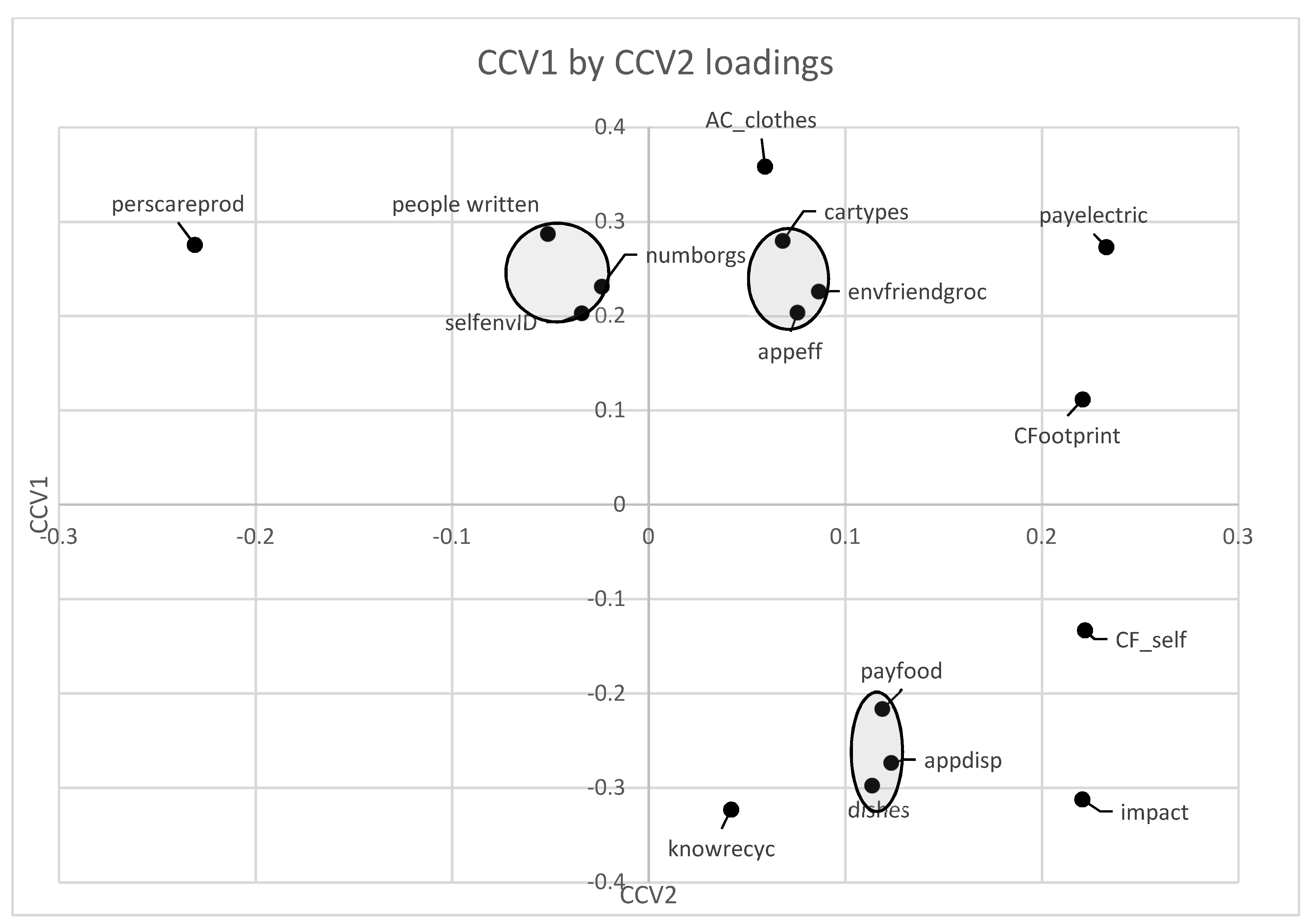
Figure 1. Graphical Representation on loadings on CCVs (Canonical Correlation Variables). In canonical correlation analysis. The corresponding items can be found in Table 1 and in the Supplementary.
Urbansci 02 00114 g001
Table 1. ERBs used in analysis.
Cluster 1
Number of different public officials a respondent indicated they had contacted with a concern in the last year
I consider myself to be an environmentalist. [5 levels, “Strongly Agree” to “Strongly Disagree”]
Number of environmental organizations an individual indicated belonging to.
Cluster 2
I try to buy environmentally friendly groceries. [1 = always, 2 = most time, 3 = half time, 4 = occasionally, 5 = never]
Number of efficient car types individuals indicated interest in buying. [Possible to select 0–3 out of 3]
Think about the last appliance you bought—TV, microwave, refrigerator, etc. When you bought this appliance, how important was energy efficiency to you in considering your options? [5 levels, “Extremely Important” to “Not important at all”]
Cluster 3
Would you be willing to pay more for your food if you knew it was grown sustainably? [Options: No, up to 10%, 25%, 50%, 75%, or double]
Think about the last time you disposed of an appliance, television, or computer. Did you dispose of it properly? [5 Levels, “Definitely Yes” to “Definitely No”]
When you do dishes by hand, or dry dishes, how often do you use reusable/cloth dish towels/dish rag? [5 levels, “Always/Almost Always” to “Never/Almost Never”]
Table 2. Description of study area, municipality means.
CharacteristicLowestHighest
Responses031
Population3800100,000
Responses/1000 population0.041.11
Land Area (acres)130030,300
Table 3. Logistic Regression summary results; * = 9.6 km circle, all else used municipal boundary.
ERBClusterLandscape Variables UsedParameter EstPr > ChiSqModel ChiSqClassification
Number of Orgs1Intercept−4.3813<0.00010.00260.655
Recreation land area *0.002120.0039
Number Written1Intercept0.43170.51270.00450.593
Total amount of water0.0001070.0063
Mean parcel to park distance−0.00050.0485
Environmentalist Self ID1Intercept−3.09680.02690.00840.623
Parcels within 1 km of park %4.64370.0153
Forest Cover *−9.35650.0477
Car Types2Intercept0.8408<0.00010.01680.597
Percent of Area in Streams *77.97090.0303
Appliance Efficiency2Intercept1.2316<0.00010.01870.574
Recreation land area *−20.8320.0203
Environmentally Friendly Groceries2Intercept0.56950.4192<0.00010.651
Mean parcel to park distance−0.000620.0136
Intersections/land area8.9810.0002
Paying more for sustainable food3Intercept−6.1735<0.00010.00750.671
Recreation land area *79.19390.0129
Proper Disposal of Appliances3Intercept5.5557<0.0001<0.00010.841
Total Road Length7.92 × 10−060.0076
Parcels within 1 km of park %−0.000670.0022
Percentage of land in Lakes *−0.03460.0069
Use of a Reusable Dish Towel3Intercept1.7942<0.00010.00490.648
Population Density−0.000130.0149
Percent of Area in Streams *96.57330.0343
Table 4. Appliance Disposal Model.
CharacteristicParameter Estimatep-value
Total Road Length7.92 × 10−060.0076
Parcels within 1 km of park %−0.000670.0022
Percentage of land in Lakes−0.03460.0069

