1. Introduction
In recent years, the accelerating pace of global climate change has drawn increasing attention from the scientific and geopolitical communities to anomalies in high temperatures. Compared to pre-industrial levels, the global average surface temperature has risen by approximately 1.1–1.2 °C, and this warming is projected to soon exceed 1.5 °C [
1]. Recent institutional projections from the Copernicus Climate Change service (C3S) and NASA further confirm that unprecedented global heat anomalies are expected by mid-century, particularly by 2025, and the longitude range of greenhouse gas concentrations across the subcontinent will also expand [
2,
3,
4]. In this scenario, extreme heat events will become more frequent, longer lasting, and more intense, severely disrupting regional climate balance. This development poses a threat to human thermal ecosystems and comfort, resulting from the combined effects of multiple climatic factors, including temperature, humidity, wind speed, and solar radiation [
5,
6].
Thermal comfort is one of the most sensitive and observable climate phenomena related to climate change; therefore, thermal comfort indices such as the Universal Thermal Climate Index (UTCI), Physiological Equivalent Temperature (PET), and the Heat Index (HI) an instrumental equivalent, an index of observational importance, are closely related to human stress levels [
7]. Climate simulation-based studies indicate that indices will increase significantly, especially under conditions of continued global warming [
8,
9].
The impact of the urban heat island effect (UHI) on the thermal comfort of urban residents is evident. Studies have shown that in densely populated urban centers and surrounding rural areas, temperature increases of up to 6 °C can lead to increased thermal stress for residents [
10,
11].
Global climate change has exacerbated the frequency, duration, and intensity of extreme thermal anomalies, posing unprecedented challenges to regional environmental stability and public health.
In the Mediterranean Levant areas, these climate shifts are aggravated thermal anomalies because of rapid urbanization, lack of water, and extreme variable topographic formation. Northwest of Jordan, which is characterized by its extreme elevation gradients and density. Population centers are especially opposed to these changeable thermal dynamics. With the rise of surrounding temperatures, the phenomenon of thermal stress is rapidly penetrating indoor environments, which directly impacts the human biological weather forecast and thermal comfort in public residential areas. Since many residents reside in naturally ventilated buildings, the understanding of continuous spatial distribution and long-range time paths of inner heat stress is no longer a theoretical inquiry but has become a critical main prerequisite for strategic municipal adaptation, energy grid flexibility, and directed public health interventions. However, a fundamental problem exists in existing literature, both at the local and regional levels: collecting detailed climate data in these complex terrains faces numerous spatial and temporal limitations. Traditional techniques rely on point climate stations, which, while providing high temporal accuracy, remain small in scale or unevenly distributed due to high construction and maintenance costs. Therefore, urban planners have had to rely on spatial interpolation techniques.
The rapid development of climate and microclimate models has enabled the accurate simulation of the impacts of climate change on thermal comfort through statistical and physical analysis, as well as models such as Weather Research and Forecasting (WRF), ENVI-met, solar radiation, and longwave environmental geometry (CMU). The application of the WRF-UCM model indicates that by the middle of this century, the urban heat stress index (UTCI) will increase by 3 to 5 °C, leading to an increase in heat stress risk and high-temperature-related mortality [
12]. SOLWEIG’s research contributes to a deeper understanding of the impact of urban planning on the thermal environment and demonstrates the necessity of mitigating urban heat stress, such as by increasing vegetation cover, improving urban planning, or using advanced urban cooling materials. Despite the ongoing development of these technologies, they overlook a crucial reality: residents spend most of their lives in buildings that absorb, store, and amplify regional climate stress to varying degrees, depending on uplift factors and the effects of local topographic shading. In northwestern Jordan, most residential buildings rely entirely on natural ventilation, and external environmental conditions are directly reflected in the living spaces. Without a spatiotemporal bridge that can reconstruct continuous internal climate indicators from finite point sources, cities will be structurally constrained in addressing energy poverty and sensitivity to internal thermal stress.
To fill this structural research gap, this study abandons loose, non-spatial mobilization methods and instead provides an advanced predictive model framework based on the separation of objective space and time. The innovative concepts and specific structural contributions of this study to existing literature can be summarized in three aspects: 1. Methodological precision, namely, distinguishing spatiotemporal correlations rather than relying on traditional standardized spatial effects; 2. Focusing on a range of fine-grained indoor building temperatures (IAT), surpassing current macroclimate assessment methods that only focus on outdoor ambient temperature (Ta). This study is based on the bioclimatic dimension of human-perceived indoor temperature in non-air-conditioned buildings; 3. Linking bioclimatic cycles to economic and social realities. The innovation of this study lies in transforming general monthly thermal trends into high-precision hourly daily variations and systematically mapping the exact times when building temperatures fall below critical heat stress thresholds (IAT ≤ 4 °C and IAT ≥ 29 °C).
Against this backdrop, this study combines geospatial technology with machine learning-based predictive models to achieve a continuous spatial assessment of thermal comfort, which is of great significance. The study contributes to filling an important searching gap by moving from traditional station-based analyses to more comprehensive spatial representation for thermal circumstances. By combining climatic interpolation, DEM, and NARX-ANN.
This frame allows us to rebuild the current thermal patterns and explore the possible future development. The result of this study supports urban and environmental planning by providing applicable insights to assess the risk of heat stress, improve climate adaptation strategies, and support decision-making in limited observational data areas. Also, the systematic frame of the study can be applicable in other areas that face similar climatic and environmental challenges.
2. Study Area
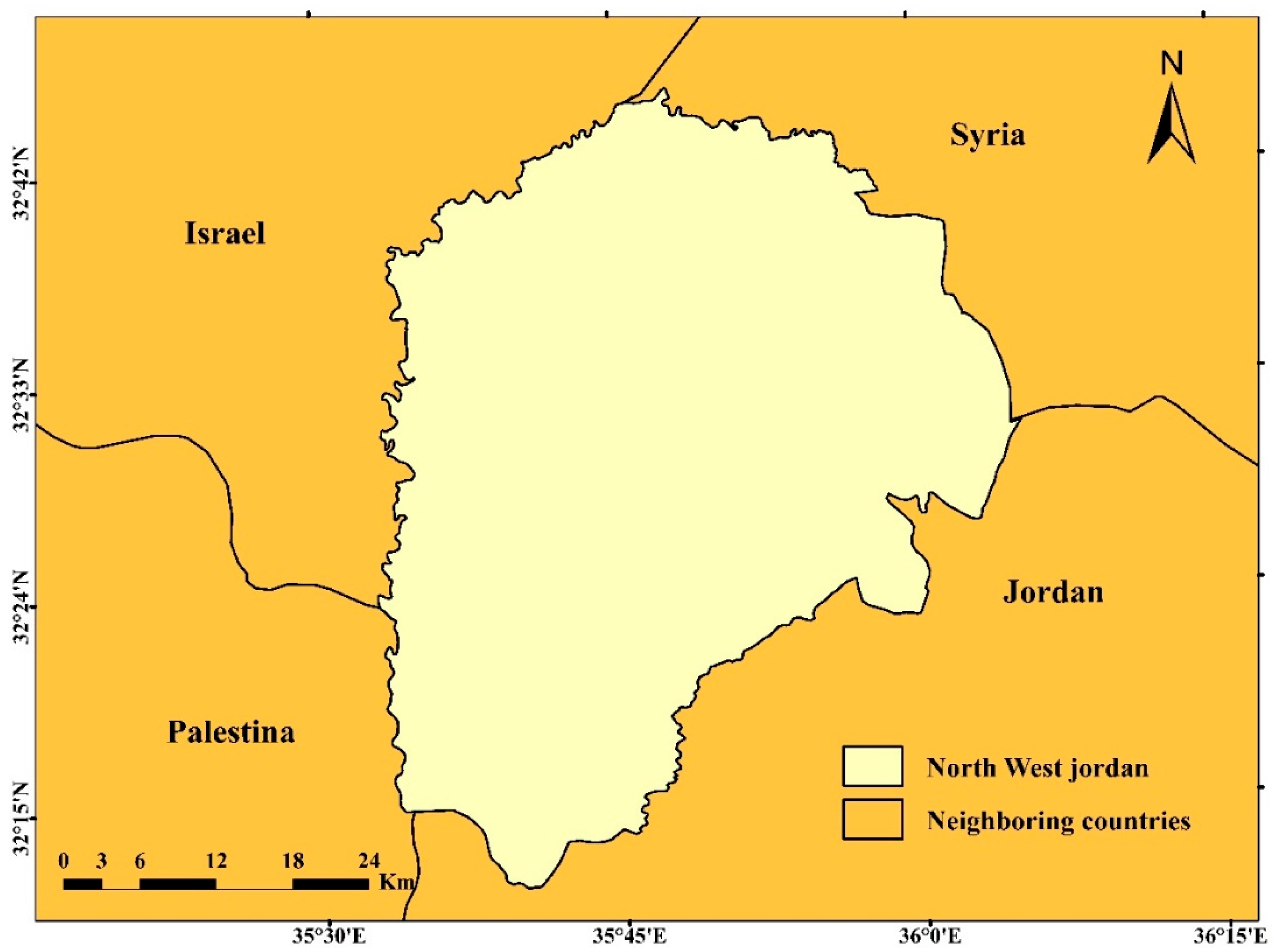
This study was conducted in the northwestern region of Jordan, located astronomically between 32°12′ S and 32°43′ N, and 35°33′ W and 35°05′ E. The study area is a populated tourist destination in Jordan in addition to the densely populated areas such as Irbid, Jerash, and Ajloun, within a relatively limited area [
13]. Geographically, it lies between the Jordan River Valley to the west and the Ajloun Highlands to the south, the Yarmouk River and the political border with Syria to the north, and the Mafraq Governorate to the east.
Figure 1 illustrates where the study area is located.
The study area boasts remarkable topographical and climate diversity, extending across a vertical elevation difference of approximately 1374 m [
14], making it one of the most environmentally and economically important regions in the Kingdom. Climatically, the area is characterized by a relatively mild Mediterranean climate compared to the other regions in Jordan, where winter is cold and rainy, and a moderate summer temperature [
15]. The spatial rainfall distribution is subjected to topographic control, as the annual rainfall average ranges from less than 200 mm in the eastern transitional steppe areas to more than 550 mm in the western mountainous highlands. Rainfall is mainly concentrated between November and March [
15,
16]; this bioclimatic diversity supports the seasonal agriculture and environmental tourism during spring and autumn when nature is green and flowery.
3. Research Methodology
The study employed several methods and tools to model the impact of climate change on thermal comfort in northern Jordan, as follows:
3.1. Digital Elevation Models (DEM)
The digital elevation model (DEM) data for this study area were obtained from the Space Shuttle Radar Topography Mission (SRTM) data provided by the United States Geological Survey (USGS). These models were projected to a coordinate system with a spatial resolution approximately 30 m.
To ensure the accuracy of spatial calculations, the projection system was converted from the geographic coordinate system to the Universal Transverse Mercator (UTM) projection system (36 zones). The digital elevation model (DEM) was then resampled to a spatial resolution of 0.5 km to process the large amount of data at the original resolution.
The coordinates of the DEM grid cells were extracted using ArcGIS 10.8 software and exported as a CSV file to simplify subsequent calculations.
3.2. Climatic Data
Jordan has a relatively limited number of weather stations, and their uneven distribution results in large areas of “climate observation gaps” [
17,
18].
This study used data from six weather stations to calculate the thermal comfort index. Data of six meteorological stations were used to do calculations of the thermal comfort index, which was obtained from the Jordan Meteorological Department. These data contained monthly temperature averages and relative humidity averages during years (1991) and (2024).
To ensure data consistency, this study employed the Standard Normality Homogeneity Test (SNHT) and the Pettitt test to detect discontinuities in the climate time series.
Table 1 clarifies stations coordinates were used in this study, height, annual rainfall average, air temperature, and relative humidity.
3.3. Spatial Numerical Procedures
Spatial interpolation is considered one of the spatial mathematical methods that enables the researcher to know geographical and topographical characteristics of the study area, especially if it is characterized by irregular distribution of spatial phenomenon climate stations.
Spatial interpolation tools contribute to forming surfaces with continuous values of spatial phenomena generated from dotted data using geographical information systems (GIS) programs. It became easier, more subjective, and higher resolution to interpolate larger areas due to expanding the use of geospatial technology, in a condition of a sufficient number of geographical dotted phenomena where the distance factor is the only variable.
However, relying solely on GIS-based interpolation can introduce significant uncertainties, especially in mountainous and complex terrains and where survey stations are sparsely or unevenly distributed. As elevation-related climate gradients [
19,
20].
Therefore, a more accurate spatial interpolation method involves developing a computation algorithm using Python that simultaneously considers the locations of neighboring sites and the vertical and horizontal gradient of climate variables across the entire landscape. The algorithm generates a dense point matrix, enabling GIS to produce a high-precision database.
Generating climate data on a spatial grid requires two main steps:
The Euclidean distance between a grid cell and a measurement station is calculated as follows:
where distance represents the Euclidean distance (in meters) between stations i and grid cell j, and x and y represent the east and north coordinates (in meters), respectively.
Air temperature for each grid cell was calculated through employing the inverse distance weighting (IDW) algorithm for spatial interpolation. As follows [
21]:
where:
x and y represent east and north coordinates (m),
z represents elevation (m),
Ti represents temperature at station i,
Γ represents the environmental lapse rate,
zi represents station elevation,
δ(i, k) represents the Euclidean distance between station i and the target grid cell.
In this study, the temperature of each grid cell was locally interpolated using data from the three most recent observation stations. Other climate variables, including relative humidity, annual precipitation, wind speed, and solar radiation, were estimated using the same method.
After spatial interpolation of temperature and relative humidity, the actual water vapor pressure of each grid cell is calculated using the following formula based on relative humidity and saturated water vapor pressure:
where actual and saturated vapor pressures are expressed in kilopascals (kPa), and RH represents relative humidity.
Saturated vapor pressure was derived using the following calculation formula [
22], where
T represents air temperature in °C:
3.4. Thermal Comfort Index
Numerous thermal comfort indices reflect the importance of studying the effects of thermal comfort on the human body. Many quantitative methods have been proposed to measure so-called thermal comfort, which refers to the suitability of climatic conditions for human comfort, or human satisfaction with the surrounding environment [
23,
24].
Thermal comfort is closely related to external factors, especially air temperature and relative humidity, as these factors significantly influence the degree of thermal discomfort experienced by individuals. This is particularly evident in buildings that are not adequately adapted to heat stress or lack proper heating systems. Many households in developing countries lack adaptation measures, and studies have shown a strong correlation between outdoor temperature and indoor environment in buildings without air conditioning. This demonstrates that thermal comfort is directly affected by external climatic factors [
25,
26].
Numerous factors influence thermal comfort, including environmental, physiological, and psychological factors, making thermal comfort modeling complex and challenging. Currently, the most accurate mathematical models for thermal comfort are those that consider heat exchange between the human body and its surrounding environment, often referred to as energy balance equations [
27,
28,
29].
Therefore, various thermal comfort indices have been developed, most of which rely on air temperature and humidity-related variables, such as relative humidity, water vapor pressure, or wet-bulb temperature (WBT) [
23,
30]. Although some indices also incorporate other environmental factors, such as wind speed and solar radiation, the main difference lies in the empirical coefficients used in each model. Observations have shown that most of these indices produce values like perceived temperature described by Steadman [
23,
31,
32].
Indices based on temperature and humidity are widely used due to their simplicity and the availability of relevant data at most weather stations. This study uses the Indoor Apparent Temperature (IAT) index because it is applicable to study under a wide range of climatic conditions. This index is applicable to a broad range of temperature and humidity and has been shown to be comparable to the Universal Thermal Index (UTCI) [
17,
18]. The characteristics and parameters used for the calculation of IAT are presented in
Table 2.
However, the vast area and complex terrain of the study region make obtaining structured metadata and building information at different building levels extremely difficult in practice. Furthermore, although this data is crucial for assessing the thermal sensitivity of buildings, a local spatial database is currently lacking. This data includes building envelope characteristics, thermal quality, shading, window-to-wall ratio, occupancy, and internal thermal gain.
Therefore, the estimation of perceived temperature is not based on actual indoor temperature records but rather serves as a geographical reference. This reflects the effectiveness of potential atmospheric thermal stress transfer between naturally ventilated buildings and their surrounding environment within the study area. Therefore, thermal comfort and the energy consumption of heating and cooling systems must be considered when estimating perceived indoor temperature (IAT).
3.5. Diurnal Thermal Comfort
Compared to annual or even monthly measurements, daily thermal comfort indices are more accurate and better represent actual climate conditions. They provide more detailed information than monthly data, which typically only offers a general overview and lacks precise details. Furthermore, daily data can detect short-term changes and fluctuations that are difficult to observe using monthly, seasonal, or annual data [
33].
Daily thermal comfort assessments provide a deeper and more detailed understanding of comfort levels. Many subtle differences are difficult to discern using monthly or yearly scales, while daily analysis reveals these variations more effectively [
34].
Therefore, calculating thermal comfort indices using daily data can identify which periods within a specific month are comfortable or uncomfortable (heat stress). This helps in accurately assessing daily heat load patterns, particularly those related to heating and cooling demands [
35].
Spectral analysis can also be used to characterize diurnal temperature variations and is an effective tool for understanding short-term climate fluctuations [
36,
37].
Here, the variable Ta(t) represents the temperature at time t. and the first term on the right-hand side if the equation represents the daily average temperature. The variable t represents time. While A
i and B
i are harmonic coefficients determined according to [
36].
This study found that using only the first harmonic coefficient is sufficient to accurately characterize daily temperature variations. Furthermore, since water vapor pressure is a conservative humidity measurement variable that fluctuates very little over short periods, it is assumed that the actual water vapor pressure remains constant throughout the entire diurnal variation cycle.
3.6. Prediction of Thermal Comfort
Time series analysis is considered one of the most important tools in climate-related research because it plays a crucial role in understanding. Describing and predicating changes in atmospheric variables such as relative humidity and temperature. Accurate forecasts are essential for climate research, including thermal comfort, thermal stress, and environmental planning.
This study employs a nonlinear autoregressive model based on an artificial neural network (NARX-ANN) for thermal comfort prediction. This model is implemented using Python (IDLE 3.11). The model is trained using historical data spanning 33 years (1991–2024) to predict future values. The dataset includes:
Monthly mean air temperature
Monthly means maximum temperature
Monthly means minimum temperature
Monthly average relative humidity
Wind speed
Monthly evaporation rate
The dataset was divided into three subsets:
85% on training
10% for validation
5% for testing
This structure enables the model to capture nonlinear relationships and time dependencies in climate time series.
The NARX-ANN method first predicts monthly values of relative humidity and temperature, then uses Python and the IAT index (as described above) to calculate thermal comfort.
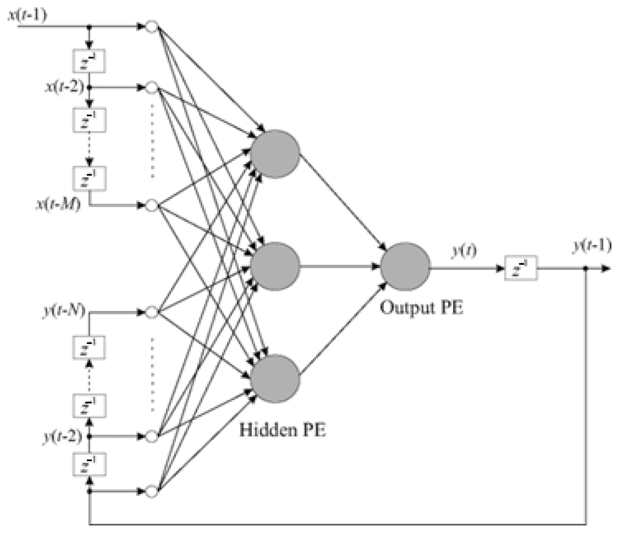
The structural topology of the NARX-ANN network is presented in
Figure 2. The model consists of three main layers:
Input Layer: where raw data (predictor variables) are introduced
Hidden Layer: where processing and training occur using complex mathematical operations
Output Layer: where the final predicted values are generated
Figure 2.
Structural topology of the NARX-ANN network.
Figure 2.
Structural topology of the NARX-ANN network.
The amount of time delay and the number of neurons in the hidden layer can be adjusted. These parameters are optimized through repeated trials to obtain the best model performance.
Future values of the time series (yt) are predicted using both:
External input variables (u)
Previous values of the same variable (y)
The term ε represents the error (or noise).
During training, the neural network approximates a function of using actual observations, representing the relationship between past and present values. This is achieved by iteratively adjusting the network weights and biases until optimal performance is reached.
Once trained, the developed model can be used to predict temperature and humidity without actual observations.
Model performance is evaluated using several statistical measures, most notably:
Mean squared error (MSE) measures the average squared difference between observed and predicted values, while R
2 represents the strength of the correlation between predicted and actual values. The lower the MSE value and the closer the R
2 value is to 1, the higher the accuracy and reliability of the model.
where:
yi represents the actual value of sample i
n represents the number of samples
ŷ represents the predicted value
ȳ represents the meaning of observed values
The NARX-ANN model is inherently designed for short- and medium-term projections, aiming to monitor potential climate change and predict future climate trends at local scales, rather than simulating long-term climate change.
Furthermore, the value of these projections should be applied in practice to support near- and medium-term urban planning and environmental management frameworks, not just adaptation to long-term climate change. Long-term future climate projections relying on regional and local scales are susceptible to high uncertainty, which can affect the results, although these projections are crucial for providing meaningful insights from a strategic planning perspective.
Short- and medium-term projections provide a system more aligned with the current planning needs of local authorities in Northwest Jordan. This aims to support resource management, infrastructure planning, and the increase and development of green space. The projected limited thermal changes are not insignificant but rather a feasible indicator of improving local resilience to future climate change within a controllable timeframe.
4. Results
4.1. Air Temperature
Outdoor temperature is a key indicator and decisive factor in determining thermal comfort and its threshold, especially in urban areas without air conditioning or relying on natural ventilation.
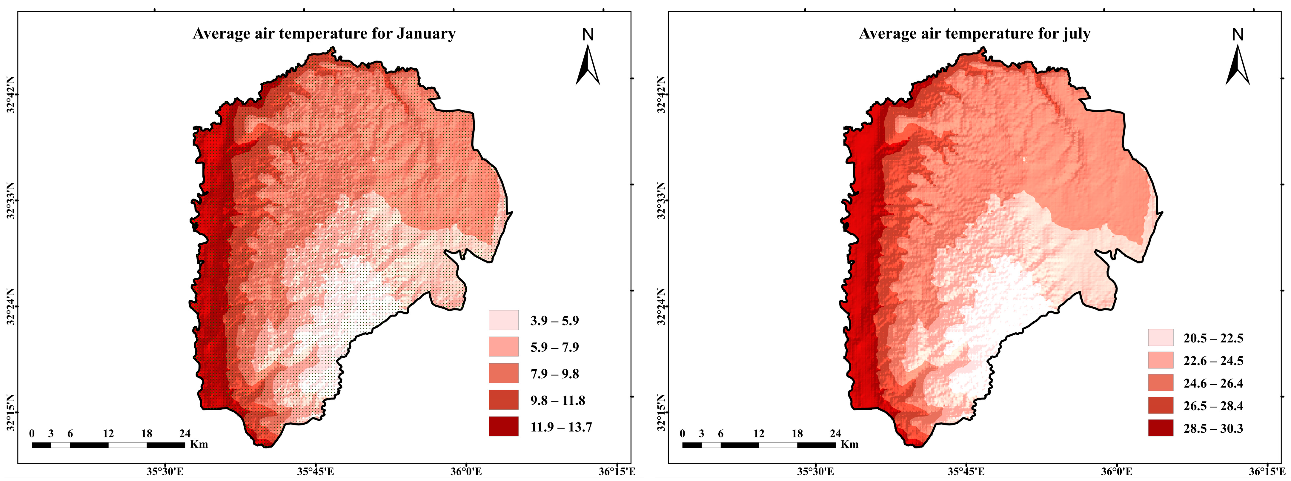
Figure 3 shows the spatiotemporal distribution of average temperatures in January and July, exhibiting two distinct seasonal peaks.
In July, temperatures gradually decrease as the study area transitions from the lower elevations of the Jordan Valley to the eastern mountains. As shown, the average temperature in the Jordan Valley reaches 30 °C in July but gradually decreases with increasing altitude. Temperatures also rise on Mount Ajlun. This significant climatic and spatial variation is likely due to the complex topographic composition (macro-topographic structure) of the study area, with the 1374-m elevation difference between the Jordan Valley and the mountains directly influencing this factor. Furthermore, the lower atmospheric pressure and air density at the mountain peaks also contribute to the cooling of the vertical adiabatic ring.
During the winter (January), the overall climate pattern maintained its geographical continuity, with temperatures in the Jordan Valley and its adjacent lowlands exceeding those in the mountains and semi-arid plains to the north and east of the study area. In January, temperatures in the Gora region remained stable at around 14 °C, while in the mountainous highlands, particularly the Ras Munif region, temperatures dropped to around 4 °C. These winter temperature variations highlight the influence of topography on the local climate, a phenomenon known as the Jordan Valley topographic-climate shelter effect, which protects vulnerable areas from extreme cold. This effect creates a localized warming zone, protecting vulnerable areas from radiated air and helping to offset the release of clod air on clear night.
4.2. Indoor Apparent Temperature (IAT)
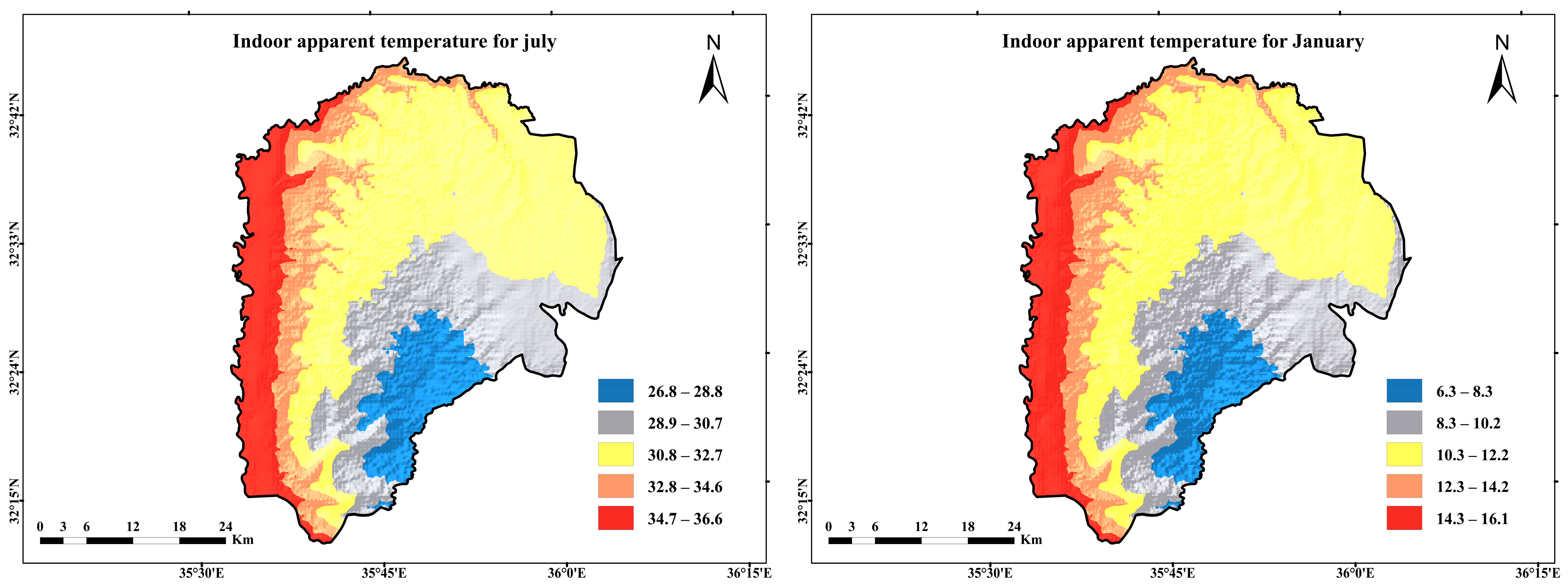
Figure 4 shows the spatial distribution of indoor perceived temperature (IAT) in the region in January and July (the empirical endpoint of the annual thermal cycle). In January, the IAT values in the Jordan Valley and its adjacent lowlands are relatively high, ranging from 14 °C to 16 °C, which, according to the IAT index, is within or slightly below the bioclimatic threshold. In contrast, the IAT values in the northern, southeastern, and highland areas of the study region are relatively low, ranging from 6 °C to 13 °C, falling into the waltz and frost categories. Based on the above analysis and from the perspective of urban energy infrastructure, the model indicates that the increase in heating intensity is more concentrated in the mountainous highlands than in the Jordan Valley and its surrounding areas. This is because the valley is below sea level, and the terrain slope forms a natural barrier, reducing the building’s reliance on electric heating. The highlands, with their steeper terrain slopes, require continuous use of heating equipment to reduce thermal stress within buildings.
During the peak summer season, represented by July, the indoor temperature (IAT) threshold exceeded 29 °C in most of the study area, with the lowest temperature recorded at 29 °C on the slopes of Mount Ajlun and 63.6 °C in the Jordan Valley. This indicates that most residential and workplace environments in northwestern Jordan require active cooling systems to maintain optimal thermal comfort conditions and avoid thermal stress, especially in enclosed spaces, as the external envelope of most traditional buildings cannot provide sufficient thermal comfort in the summer. This leads to increased electricity consumption and energy load, as cooling living spaces has become a public health necessity, not just a luxury. However, at higher altitudes, climate adaptability is better, with lower indoor temperature values falling within a slightly warmer range, with indoor temperatures at 26 °C on the mountaintop and 28 °C at the foot of the mountains. This suggests that, given the thermal safety provided by urban topography, continuous use of cooling systems in urban centers is not necessary.
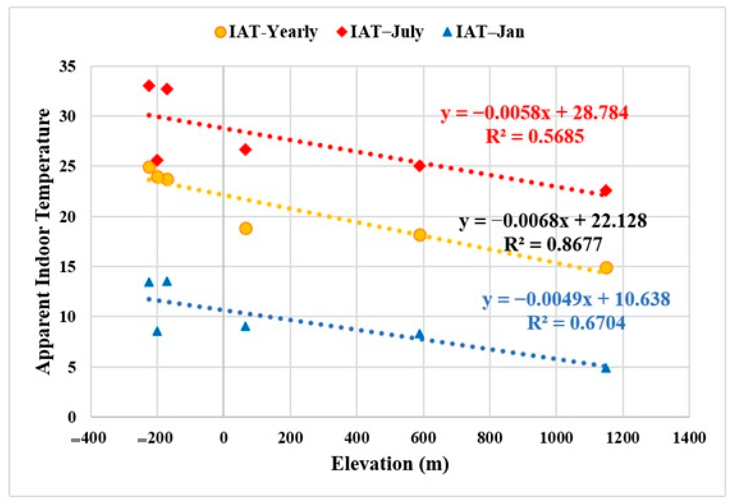
To validate the results of the mathematical and map analyses, we conducted a local linear regression analysis. The results confirmed that topographic elevation was the most significant controlling factor affecting indoor perceived temperature (IAT). Mathematical results from the experiment confirmed a significant negative correlation between topographic elevation and IAT values, with coefficients of determination (R
2) of 0.67 and 0.57 in January and July, respectively. Furthermore, the experimental data showed a significant seasonal variation in the rate of decrease in IAT values, increasing from 0.49 °C/100 m in January (y = −0.0049x + 10.638) to 0.58 °C/100 m in July (y = −0.0058x + 28.74), as illustrated in
Figure 5. The increased rate of decrease in vertical ambient temperature during summer is due to increased sensible heat flux, enhanced solar radiation, and complex convection processes (e.g., intense solar radiation heating in open areas with complex terrain during the summer solstice), leading to strong thermal differences between depressions and highlands.
4.3. Diurnal Thermal Comfort
Diurnal thermal comfort cycles are more precise in time than menstrual cycles, allowing us to distinguish numerous details within short periods of the day. This is because thermal comfort assessments based on the time precision of menstrual cycles are inaccurate and often mask the strong and frequent anomalies that determine and control the body’s true bioclimatic stress. Diurnal cycle analysis not only provides detailed temporal precision but also helps us identify the main thermal comfort zones within a day and within a specific month. This helps identify or estimate the energy required for adaptation or cooling and determines productivity based on safe outdoor activities and their corresponding duration.
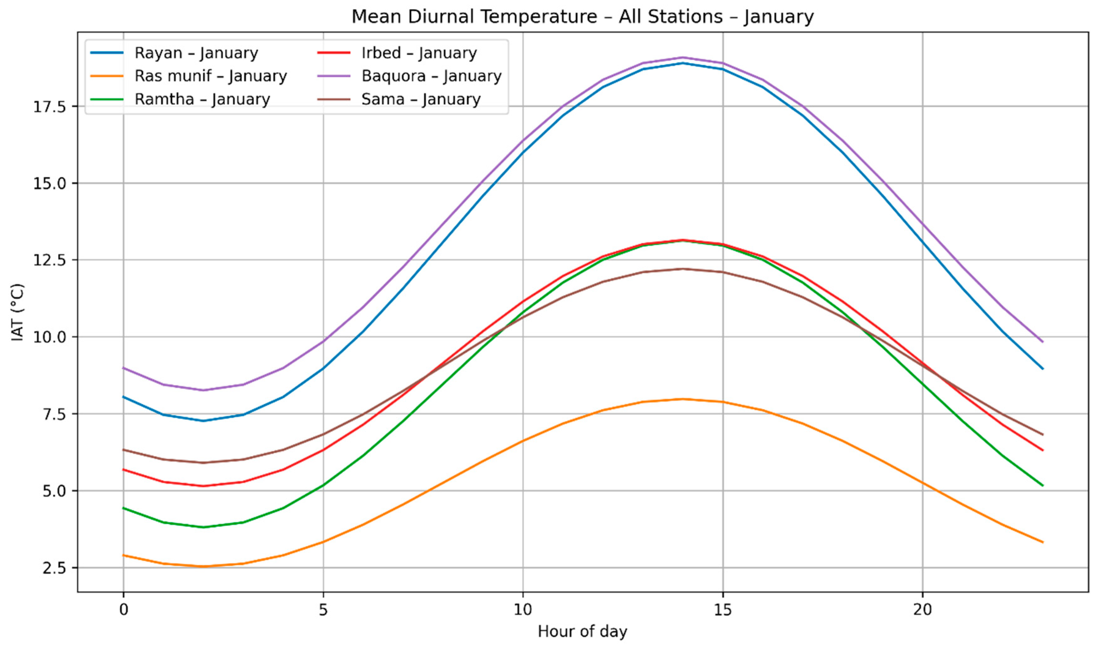
Table 3 shows the number of hours corresponding to given indoor air temperature (IAT) values at six weather stations in densely populated areas in July and January. From the table, the following points can be derived regarding thermal comfort in January (typically representing winter):
It is noteworthy that, except for the exceptional climates of the Jordan Valley and Wadi Al-Rayyan, buildings were generally cold or extremely cold. The Ras Munif weather station recorded the coldest weather, with indoor temperatures below the 13 °C threshold for 24 h. This was followed by the Ramtha weather station (23 h), and the Irbid and Sama weather stations (both 22 h) in the eastern and northern plains.
These prolonged periods of cold weather at these stations likely indicate insufficient or complete absorption of passive solar energy within buildings during the day, explaining why continued fuel consumption leads to energy poverty and exacerbates the economic burden on residents in these regions. For example, in the Jordan Valley (represented by the Wadi Al-Rayyan and Baqoura stations).
Table 3 shows a sharp drop in the number of hours with average indoor temperature (IAT) below 13 °C, reaching only a warm and comfortable environment for half of the day’s winter cycle without any heating, clearly demonstrating the regional differences in urban energy load (see
Figure 6).
For July (summer conditions), the following observations can be made based on
Table 3:
1. The Jordan Valley, especially its northern region, enjoys suitable thermal comfort conditions, with no heat or cold stress. Only brief periods of slight cold occur near the Wadi Al-Rayyan and Al-Baqoura weather stations, where indoor temperatures below 8 °C occur for only one hour each day.
The winter thermal characteristics of the Jordan Valley differ from the overall pattern of the study area, making it a vital economic, social, and strategic hub for Jordan. From a bioclimatological perspective, the region’s low altitude creates a subtropical climate in the mid-latitudes, making winters ideal for tourism, recreation, and picnics. This thermal stability also ensures the sustainable development of its agricultural resources, supplying fresh fruits and vegetables to Jordanian domestic and export markets during the peak winter season.
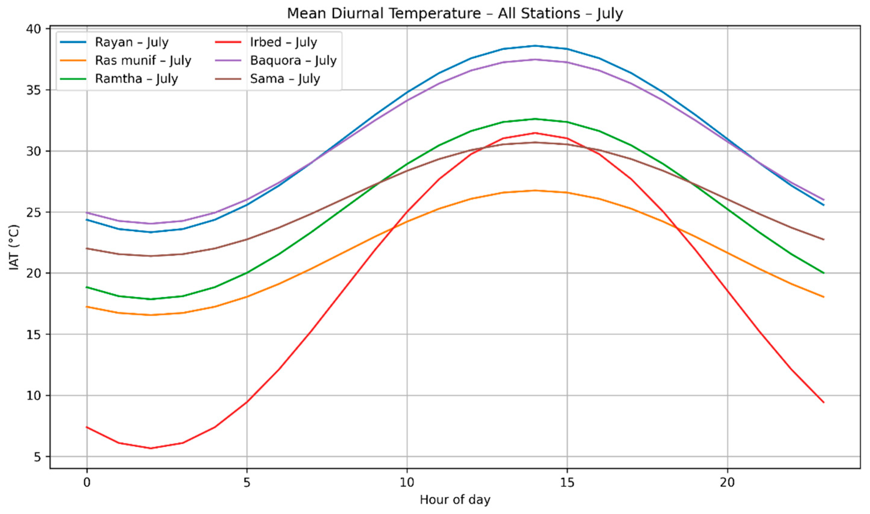
Focusing on the peak summer conditions typically represented by July, the following conclusions can be drawn from
Table 3. We note that the Jordan Valley region is witnessing cases of heat stress, where the atmosphere is very hot during the day and where the calculation of thermal comfort dominates the entire daily cycle, as IAT values continue above the threshold of 29 degrees for 24 h without stopping. This causes continuous and uniform thermal discomfort for the residents of the region and deprives them of any space for nocturnal relief, which requires the provision of means of adaptation in both residential and office buildings, and therefore it is necessary to invest in electrical energy to achieve the comfort of the residents of the area.
Table 3 and
Figure 7 show that the internal air temperature in the Jordan Valley during July exceeds 35 °C throughout the day, causing significant heat stress, especially during working periods.
2. Other parts of the study area, whether the plains where Irbid and Ramtha are located or the mountainous areas where Ajlun and Jerash are located, experienced moderate to severe heat, primarily concentrated in the afternoon. At Ras Munif station, the duration of temperatures exceeding 29 °C and 26 °C was only 1 h and 8 h, respectively.
3. Other parts of the study area, whether the plains (Irbid and Ramtha) or the mountains (Ajlun and Jerash), experienced varying durations of high to extremely hot weather throughout the day.
For example, at Ras Munif station, the temperatures exceeding 29 °C and 26 °C in July were approximately 1 h and 8 h, respectively. At Sama station, these figures increased to 8 h and 14 h, respectively.
These climatic conditions lead to increased periods of thermal discomfort in urban centers, affecting a significant portion of the population, especially in buildings lacking air conditioning systems. Therefore, increased electricity consumption for air conditioning is expected to be necessary to achieve thermal comfort.
4.4. Predicted Thermal Comfort
Climate factor prediction is one of the most important research directions and a cornerstone of modern applied climatology, as it is directly and indirectly related to human adaptability in the context of accelerating global warming. Among these factors, the prediction of thermal comfort is a key focus of applied climatology and urban climatology research because of the complex relationships and interactions between climate factors, urban characteristics, and human behavior.
Especially after the Intergovernmental Panel on Climate Change (IPCC) released its global warming scenario prediction report, the development of efficient simulation models to predict the thermodynamic characteristics of urban environments had become particularly urgent. Tracking local thermal changes is no longer just an analytical tool but a crucial predictive tool for urban planning, mitigating public health risks, and designing sustainable infrastructure.
The prediction of thermal comfort is also vital at the health and economic levels, helping to understand the duration of people’s exposure to thermal stress and the low economic productivity of workers in various production sectors. Predicting expected thermal rest patterns also helps to understand and determine energy consumption and peak periods. Therefore, prediction is not only an analytical tool but also one of the pillars supporting planning decisions and achieving environmental and economic sustainability.
4.4.1. NARX-ANN Model
To simulate the nonlinear interactions of complex climates, this study employs a spatiotemporally decoupled prediction model framework based on Artificial Neural Networks (ANNs), specifically the Nonlinear Autoregressive Network Algorithm (NARX) with external input.
The optimal prediction structure of the model was obtained through a Multilayer Perceptron (MLP) configuration containing 64 effective neurons and two hidden layers, each containing 32 effective neurons, combined with a 24-step feedback delay. The training period was limited to a maximum of 800 epochs, controlled by an EarlyStopping algorithm that terminated training immediately when the validation loss stopped decreasing, thus mitigating the risk of overfitting caused by pointwise predictions.
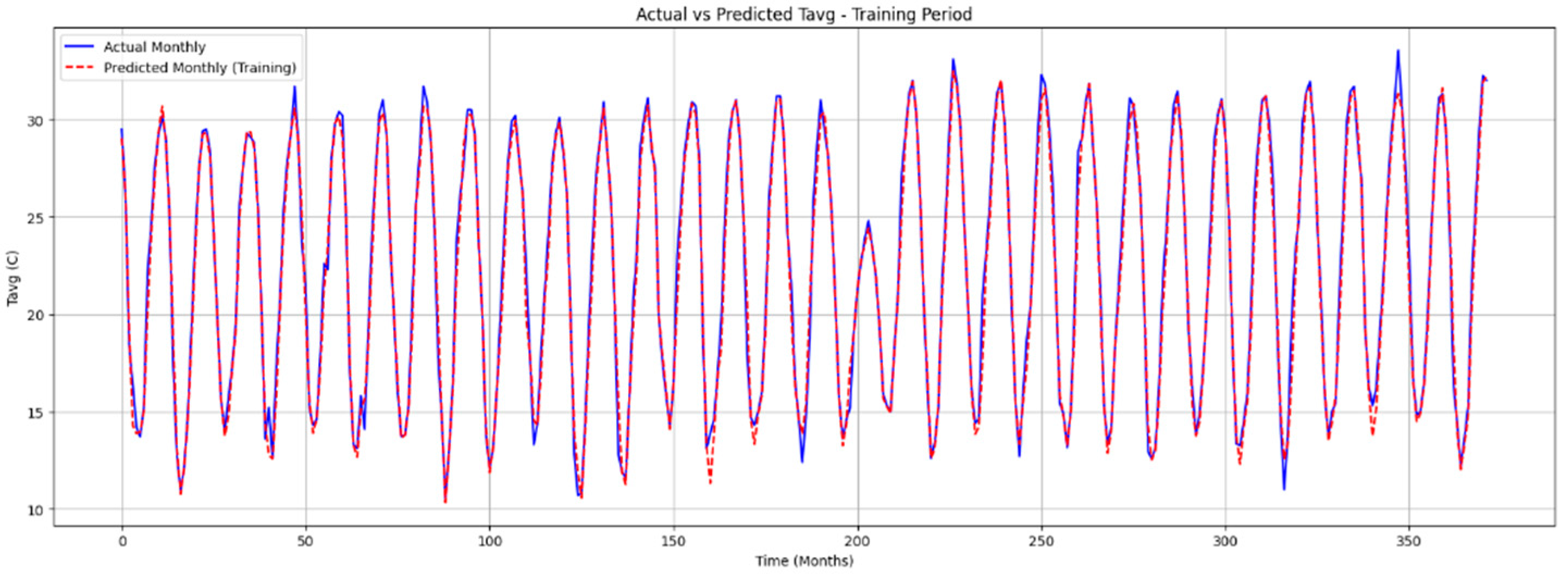
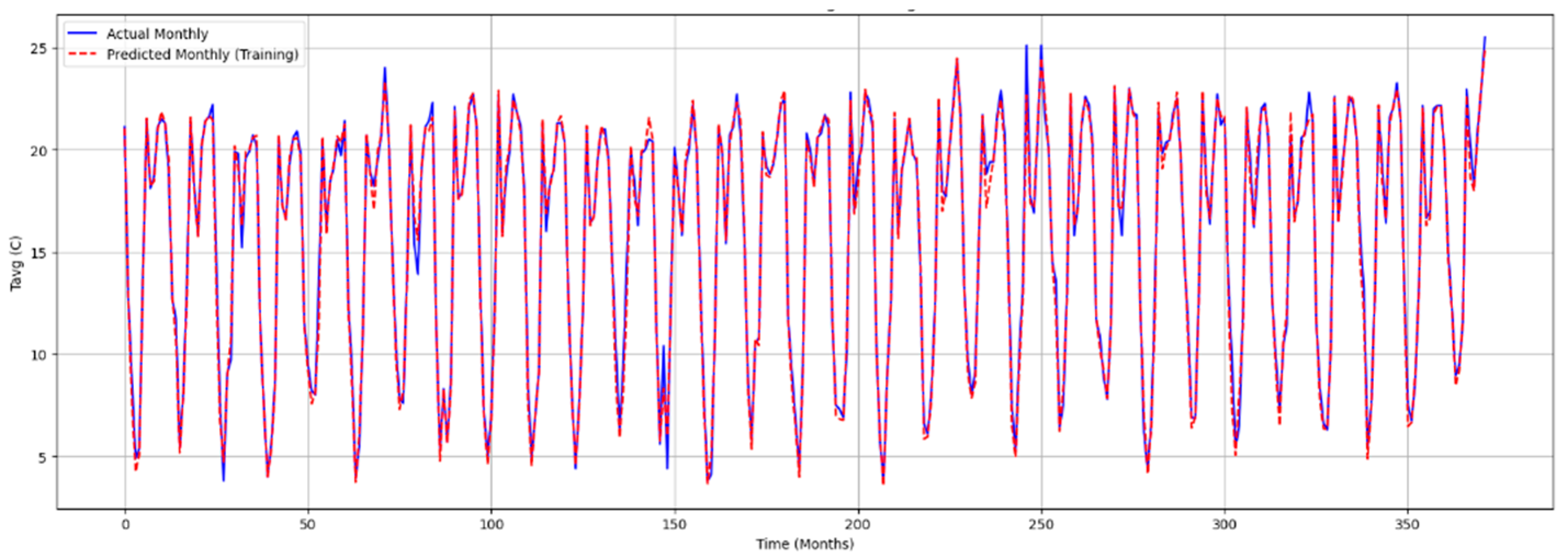
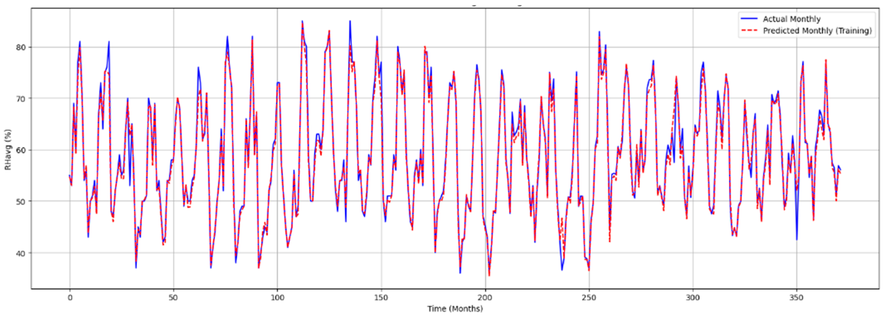
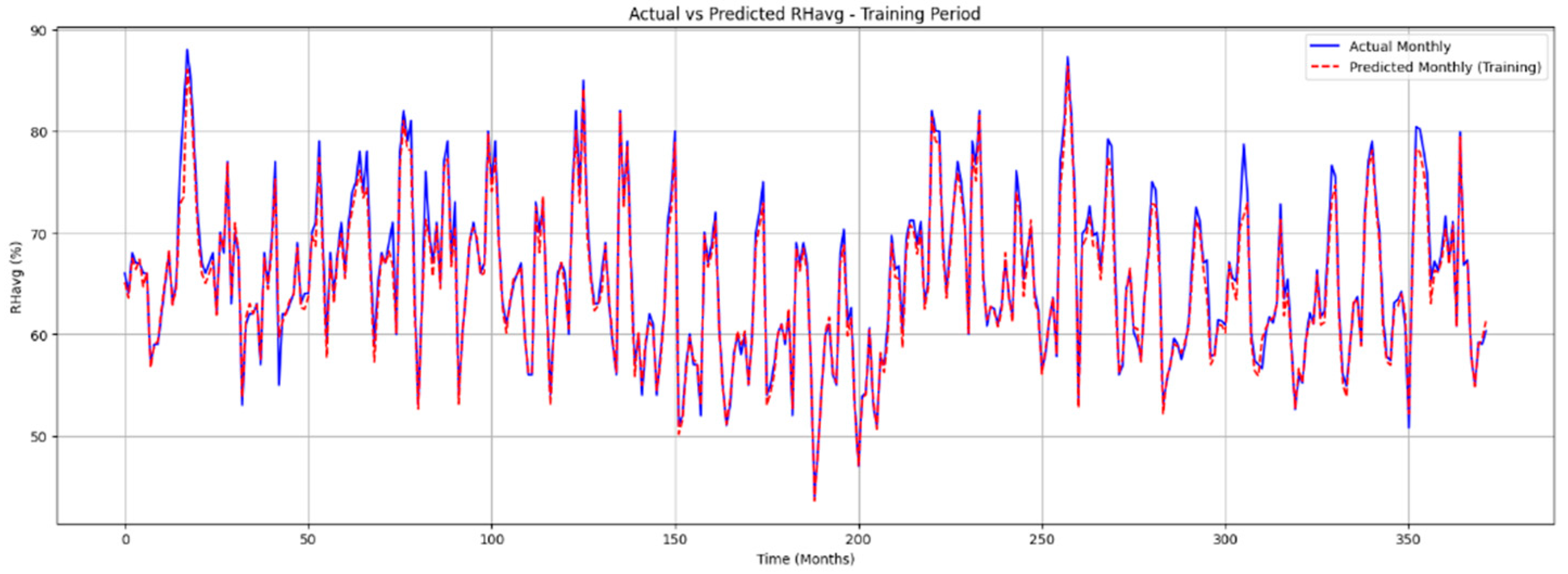
Although the model relies on time series implemented at the climate station level and doesn’t explicitly integrate topographic spatial relationships, it demonstrates high efficiency in estimating local climate details, especially when combined with categorical spatial interpolation techniques within a Geographic Information System (GIS) environment. The model achieves a near-perfect simulation of historical experimental data trend lines, with a coefficient of determination (R
2) ranging from 0.95 to 0.98, indicating good stability and demonstrating its ability to explain spatiotemporal variations. Mean squared error (MSE) results show high predictive accuracy, with values ranging from 0.35 to 0.50.
Figure 8,
Figure 9,
Figure 10 and
Figure 11 illustrate the results of training the NARX-ANN model using temperature and humidity sample data from the Sama and Al-Baqoura plants, validating the mathematical reliability of the decoupled model framework before making predictions for the next decade.
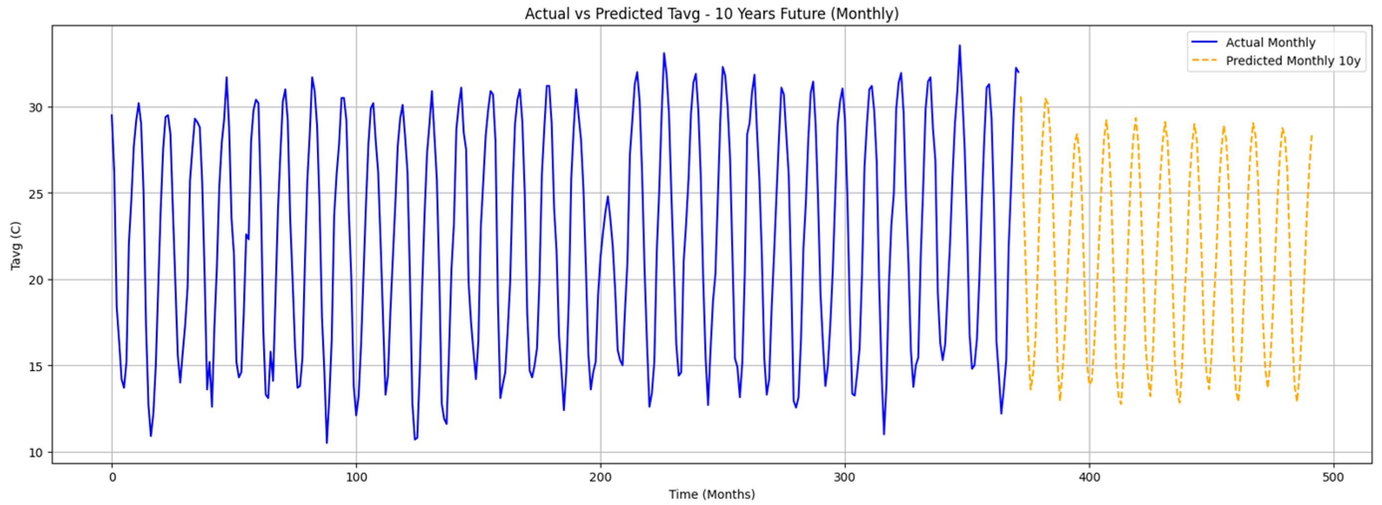
It is worth emphasizing that the prediction accuracy obtained using this model, reflected by an R2 value of approximately 0.95, was obtained during the training and testing phase on scattered historical data from 1991 to 2024, rather than for a 10-year prediction period. This is because errors and uncertainties naturally accumulate and increase in nonlinearity, random variation, and systematic climate anomalies, so future mathematics may not be consistent with historical mathematics.
Therefore, this study employs the NARX-ANN model as an improved forecasting tool. The model’s feedback loops and external climate associations are specifically designed to reduce error inflations in the short to medium term, thus providing a context-based reference framework for regional climate adaptation rather than absolute certainty.
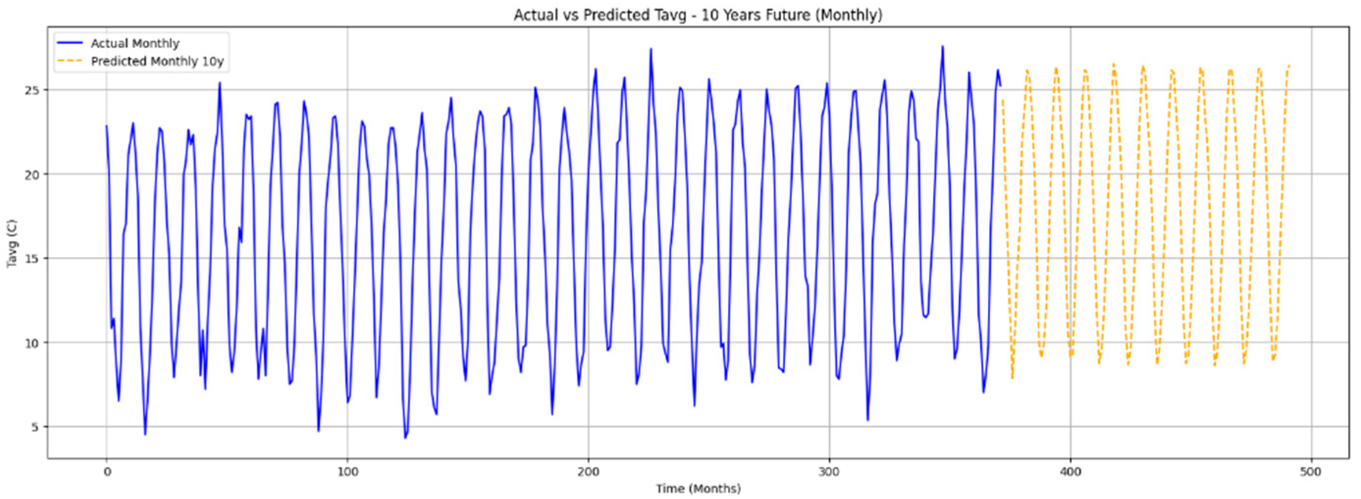
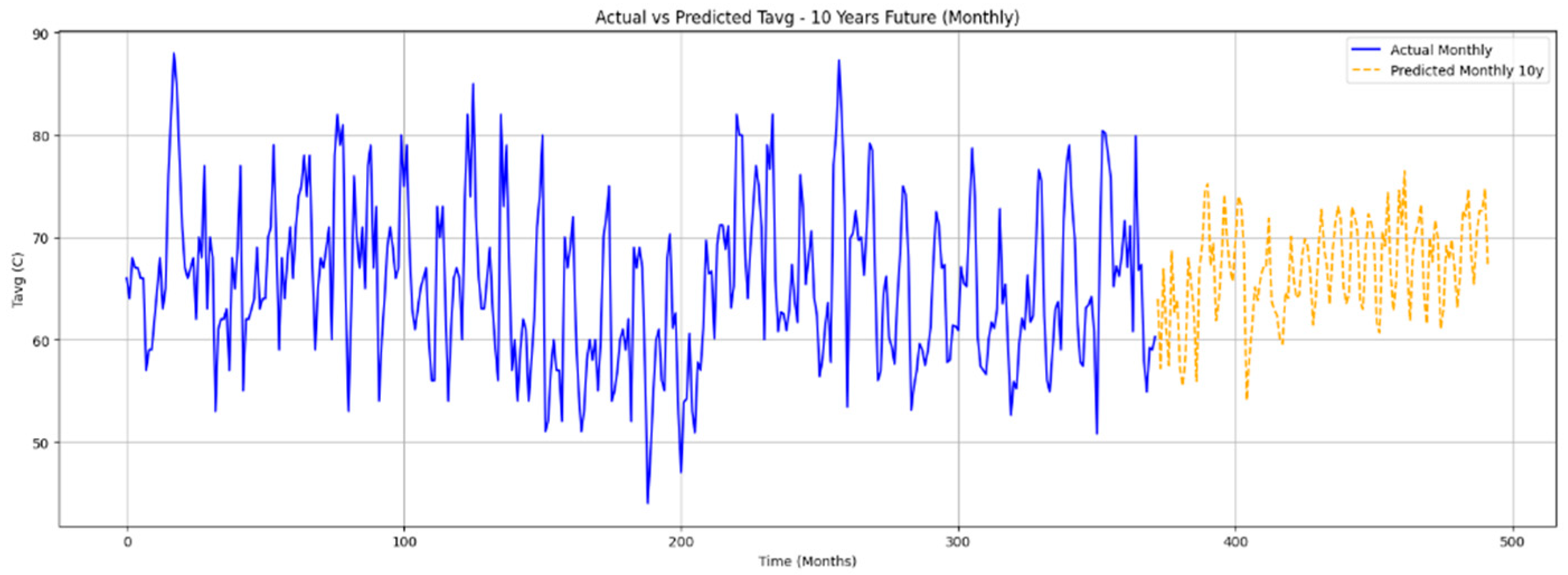
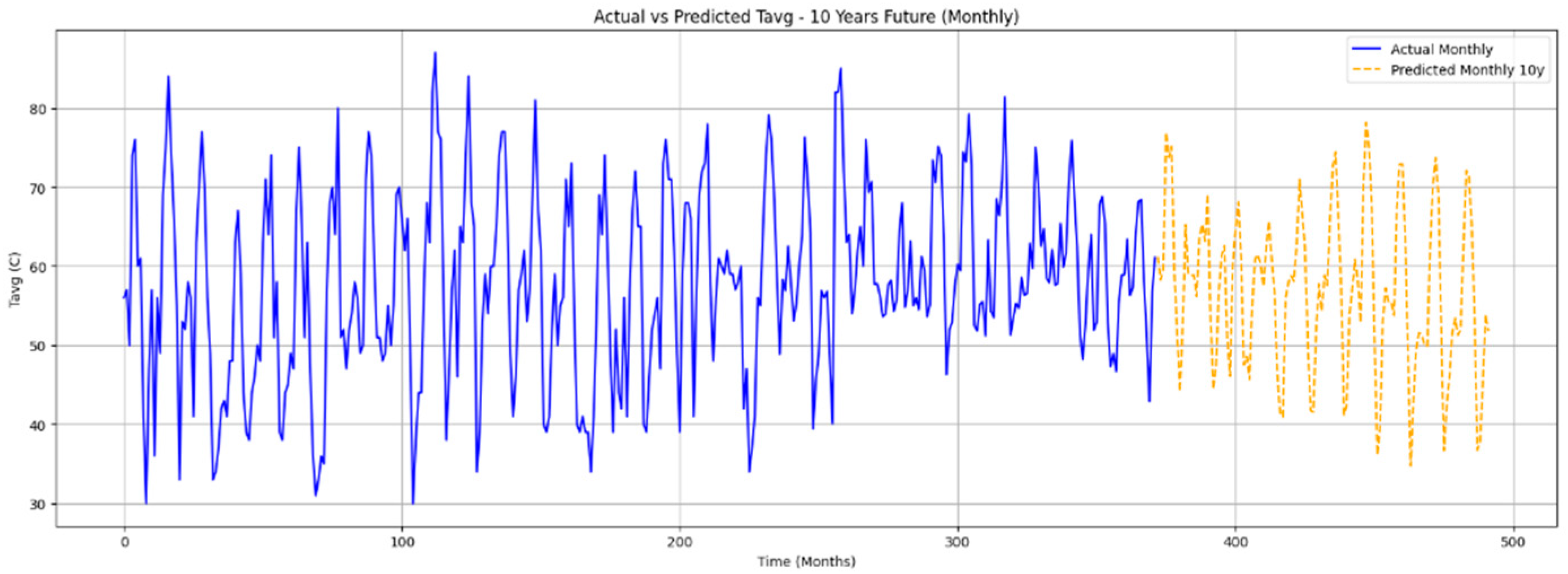
Using existing data for forecasting is crucial for validating the method’s correctness and the model’s accuracy. However, this study aims to extend this method to predict future values for a specific period (i.e., 10 years after the last available temperature and humidity data).
Figure 12,
Figure 13,
Figure 14 and
Figure 15 illustrate the 10-year forecast results.
4.4.2. Predicted Air Temperature
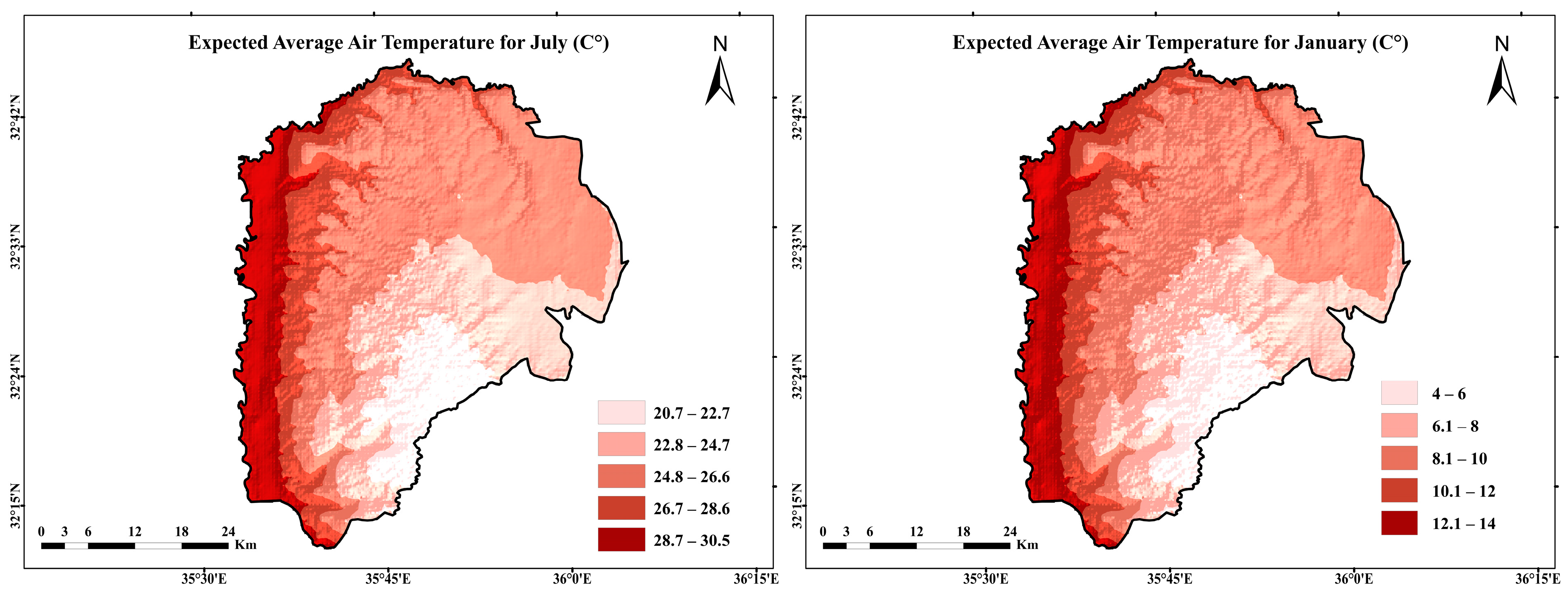
Figure 16 shows the spatial distribution of the expected average temperatures for January and July. We note that temperature differences persist between the east and west and between the north and south of the study area when predicting monthly average temperatures; that is, the current spatial variation pattern is not significantly different from the predicted values. This indicates that the overall climate topography of the region will continue to dominate the spatial distribution of temperature, maintaining the pattern observed in historical data. Algorithm results show no difference between the current and predicted monthly average temperatures, as shown in
Figure 16. Temperatures in the Jordan Valley will remain around 14 °C, while in the mountains, particularly in the Ras Munif region, temperatures will drop to approximately 4 °C.
During the summer, the NARX algorithm predicts a slight upward trend in absolute values. According to the numerical predictions from the NARX algorithm, the expected monthly average temperature in the Jordan Valley in July will rise, reaching a maximum of approximately 31 °C along the valley floor, before gradually decreasing eastward to 21 °C in the Ajlun Highlands.
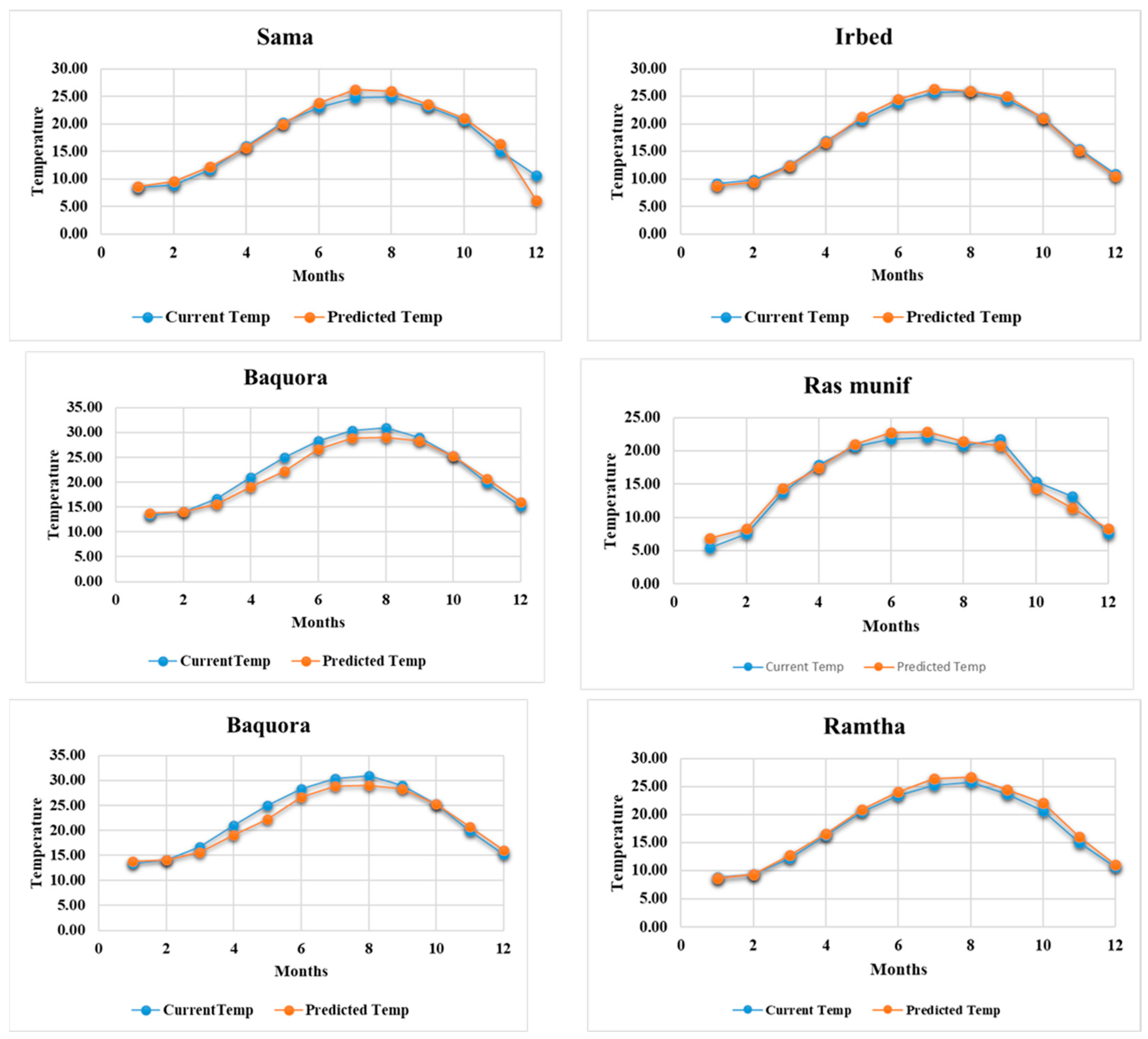
Figure 17 also details the monthly variations in current and expected average temperatures at various stations within the study area. The figures show that the monthly average values of expected and actual average temperatures at each station are relatively close. The largest negative anomaly between the expected and current values at the Wadi Rayan station is less than −1.40 °C, meaning that the expected value for that month at that station is lower than the current value.
The positive anomaly at Ramtha reached its peak (+1.50°), meaning the expected value was higher than the actual value for the month. This localized change highlights subtle differences in climate: weather stations in Jordan Valley benefit from local climate barriers and buffer zones, thus mitigating warming, while weather stations in the semi-arid open plains of Ramtha face accelerated continental warming, which may also be related to insufficient vegetation cover and land degradation +1.5 °C.
4.4.3. Predicted Indoor Apparent Temperature (IAT)
Using Python, a map representation of the expected IAT output was generated via the NARX algorithm. Using GIS technology, specifically ArcGIS 10.8 software,
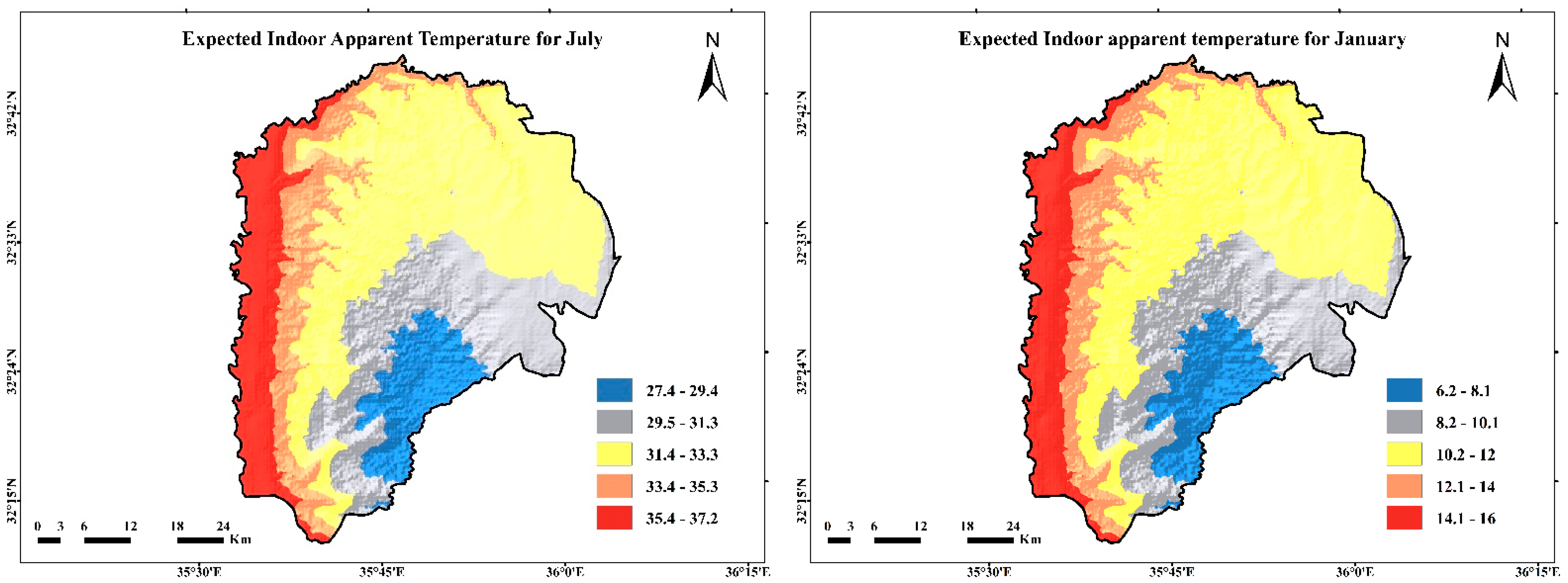
Figure 18 shows the spatial distribution of the predicated virtual interior temperature for January and July (as the endpoints of the annual cycle). During winter, the predicted IAT values didn’t show any statistically significant deviation from historical climate records, as the peak IAT in the valleys remained between 14° and 16°, indicating a slight cooling trend.
Indoor perceived temperatures in the northern, northeastern, southeastern, and highland areas of the study region are projected to drop to cold or moderately cold, with indoor temperature (IAT) values ranging from 6 °C to 13 °C, like current indoor temperature index readings. Therefore, these projections reinforce expectations for short- to medium-term infrastructure planning, as heating demand in high-altitude mountainous areas will continue to be higher than in the Jordan Valley, resulting in higher heating energy loads and consumption. This necessitates policies supporting the use of energy-efficient insulation materials in buildings to fundamentally reduce the sensitivity of local heating networks.
On the other hand, the spatial variation of the IAT index in July reflects the summer conditions overall. The results show that the index value exceeded 29 °C in most parts of the study area, indicating a similarity in spatial variation between current and predicted IAT values. However, the expected summer IAT index value is slightly higher than the current value, reaching 37.2 °C in the Jordan Valley, but still falling into the high-temperature category. An IAT index value higher than the current value of 27.4 °C is only observed in the Ras Munif station and the Ajlun Highlands region.
Based on the above analysis, the NARX study indicates that regions historically protected from extreme heat due to their high altitude are undergoing anticipated changes and beginning to face increasing thermal stress. This serves as a clear early warning to urban planners and policymakers: residential and commercial buildings in northwestern Jordan must be retrofitted with climate-adapted cooling systems and green roof technologies. Failure to implement these policies and spatial interventions will inevitably lead to increased power outages and overloads and exacerbate public health risks during future heat waves.
5. Discussion and Conclusions
One of the obstacles and challenges facing developing countries is the need for accurate climate analysis to support policymakers and environmental and urban planning processes. This deficiency may stem from a relative lack of high-resolution climate data in these countries. This data is a key element in assessing many practical applications, such as urban planning and supporting programs, environmental resource management, estimating energy demands for heating and cooling, and studying the impacts of climate change on residents’ thermal comfort. This requires a radical transformation in how climate data is processed, analyzed, and spatially represented.
Thermal comfort is typically assessed based on point measurements from meteorological stations. This approach fails to accurately characterize spatial climate, especially in topographically complex regions. This study employs a spatiotemporally decoupled prediction framework that integrates geospatial techniques, statistical analysis models, and an advanced artificial neural network architecture (NARC-ANN) to generate spatially continuous climate data with high spatial resolution for estimating the virtual indoor temperature index (IAT).
The results indicate significant spatiotemporal variations in thermal comfort levels and values in northwestern Jordan, suggesting that climate change and topographic factors have influenced the distribution and changes in the thermal environment of the study area. Mapping and mathematical analysis confirm the significant and decisive role of altitude as a spatial controlling factor. The Ras-Munif meteorological station. Located at an altitude of 1150 m, recorded the most extreme winter climate, with indoor temperatures remaining below the threshold of 13 °C for 24 consecutive hours, including 12 h below the extreme low-temperature threshold of 4 °C.
These findings can be interpreted through the lens of human biometeorology; as established by Matzarakis et all such thermal conditions are driven by the modulation of radiation flux densities, which are highly sensitive to topographical elevations. When viewed in relation to broader epidemiological evidence, these findings carry significant implications for public health [
38]. Consistent with global observations by Gasparrini et all, our study highlights that persistent exposure to these low ambient temperatures is a critical risk factor for mortality and morbidity. Specifically, the documented IAT values indicate that populations in high-altitude zones are subjected to prolonged cold stress, which is well-established to induce cardiovascular and respiratory complications through physiological mechanisms such as elevated blood pressure, increased blood viscosity, and attenuated thermoregulatory responsiveness [
39]. Thus, the sustained cold stress in Jordan’s highland regions represents a substantial, yet often overlooked, health burden that necessitates targeted interventions based on both microclimate modeling and resilient public health planning.
This persistent heat stress places a financial burden on households, exacerbating energy poverty due to continued reliance on heating. In contrast, the Jordan Valley and its surrounding areas enjoy the highest winter comfort levels, with only 12 h of cold weather, creating naturally warm days. However, indoor air temperature (IAT) tests show that values rise during the summer, particularly in July and August, indicating that people are more susceptible to heat stress during this period, especially in densely populated urban areas.
Linear regression models confirmed these results, demonstrating the existence of seasonal variation. The acceleration factor for vertical heat loss increased from −0.49 °C per 100 m in January to −0.58 °C per 100 m in July. This enhanced summer physicochemical trend is likely due to the expanding heat flow and complex convection processes over exposed terrain, along with intense solar radiation, widening the thermal gap between warmer lowlands and shallower mountainous areas. Overall, the findings are consistent with the climate literature, which indicates that lying areas and built-up areas are most vulnerable to thermal stress due to the combined effects of climate and urban topographic factors.
The techniques and methods employed in this study offer several significant operational advantages, enhancing the ability to process and simulate high-resolution bioclimatic data in complex geographical environments. The main mathematical advantage of NARX-ANN lies in its iterative feedback-based architecture and delayed step mechanism, which captures the influence of complex and nonlinear climate memory values and the inherent time intervals in precise local climate time series, thereby improving the accuracy of temporal predictions to a statistically excellent level. Furthermore, the model effectively integrates external stimulus variables, enabling it to self-correct its prediction trajectory over a longer period (1991–2024). Finally, this NSW spatial interpolation prediction method based on a GIS environment and an improved digital elevation model avoids the enormous computational burden and complex coefficient requirements of traditional physical models (such as WRF or ENVI-MET), providing an economical and scalable computing solution for data-scarce developing regions.
In contrast, a rigorous scientific evaluation needs to recognize the structural limitations of the techniques used in this study. The basic algorithmic structure of the NARX-ANN model is based on location-specific time-series operations, meaning that it does not explicitly integrate spatial terrain relationships or geographically weighted learning mechanisms during the artificial cell network optimization stage. Therefore, the geographic reliability of continuous local maps is still structurally limited by the deterministic or statistically deterministic assumptions of spatial interpolation techniques in the subsequent GIS environment. This may lead to local smoothing effects on highly refractive terrain, potentially amplifying or slightly reducing microthermal differences.
Based on the findings, spatial analysis has a significant advantage in studying the anticipated impacts of climate change on urban areas because it can identify regions most vulnerable to heat stress.
Therefore, this study recommends incorporating these findings, along with the outputs of regression models and decoupled neural networks, into Jordan’s current urban planning and energy management policies to enhance urban resilience to climate change. Appropriate building standards should be developed to accommodate these extreme topographical variations. Furthermore, high-resolution spatial analysis should be utilized to identify heat stress hotspots, thereby enhancing the resilience of the built environment and its ability to adapt to anticipated climate change scenarios.
Author Contributions
Conceptualization, A.A.G.; methodology, A.A.G.; software, A.A.G. and E.M.K.; validation, A.A.G., F.M.A. and A.M.T.; formal analysis, A.A.G., F.M.A., A.M.T. and E.M.K.; investigation, A.A.G., K.A.A.A.M., H.M.B.K. and B.A.K.; resources, A.A.G., F.M.A., A.M.T., E.M.K., B.A.K., K.A.A.A.M., H.M.B.K. and G.L.A.; writing—original draft preparation, A.A.G., E.M.K. and G.L.A.; writing—review and editing, A.A.G., E.M.K., G.L.A., F.M.A., A.M.T., K.A.A.A.M. and H.M.B.K.; visualization, A.A.G. and E.M.K.; supervision, A.A.G., E.M.K. and A.M.T.; project administration, A.A.G., F.M.A., A.M.T., E.M.K. and H.M.B.K. All authors have read and agreed to the published version of the manuscript.
Funding
This research received no external funding.
Data Availability Statement
The original contributions presented in the study are included in the article. Further inquiries can be directed at the corresponding author.
Conflicts of Interest
The authors declare no conflict of interest.
References
- IPCC. Summary for Policymakers. In Climate Change 2021: The Physical Science Basis; Masson-Delmotte, V., Zhai, P., Pirani, A., Connors, S.L., Péan, C., Berger, S., Caud, N., Chen, Y., Goldfarb, L., Gomis, M.I., et al., Eds.; Contribution of Working Group I to the Sixth Assessment Report of the Intergovernmental Panel on Climate Change; Cambridge University Press: Cambridge, UK, 2021; pp. 3–32. [Google Scholar]
- Copernicus Climate Change Service (C3S). Global Climate Highlights 2024–2025: Tracking Thermal Anomalies; European Centre for Medium-Range Weather Forecasts (ECMWF): Reading, UK, 2025. [Google Scholar]
- Intergovernmental Panel on Climate Change (IPCC). Climate Change 2023: Synthesis Report; Core Writing Team, Lee, H., Romero, J., Eds.; Contribution of Working Groups I, II and III to the Sixth Assessment Report of the Intergovernmental Panel on Climate Change; IPCC: Geneva, Switzerland, 2023. [Google Scholar]
- NASA Goddard Institute for Space Studies (GISS). Global Temperature Anomalies and Projected Trends for 2025; NASA: New York, NY, USA, 2025.
- Fiala, D.; Havenith, G.; Bröde, P.; Kampmann, B.; Jendritzky, G. UTCI-Fiala Multi-Node Model of Human Heat Transfer and Temperature Regulation. Int. J. Biometeorol. 2012, 56, 429–441. [Google Scholar] [PubMed]
- Havenith, G.; Fiala, D. Thermal Indices and Thermophysiological Modeling for Heat Stress. Compr. Physiol. 2016, 6, 255–302. [Google Scholar] [CrossRef] [Scilit]
- Chen, L.; Ng, E. Outdoor Thermal Comfort and Outdoor Activities: A Review of Research in the Past Decade. Cities 2012, 29, 118–125. [Google Scholar] [CrossRef] [Scilit]
- Zhang, Y.; Li, X.; Chen, D. Impacts of Climate Change on Outdoor Thermal Comfort and Heat Stress in Urban Environments. Build. Environ. 2021, 196, 107791. [Google Scholar]
- Li, D.; Bou-Zeid, E.; Oppenheimer, M. The Effectiveness of Cool and Green Infrastructure for Mitigating Urban Heat Stress under Climate Change. Environ. Res. Lett. 2020, 15, 114004. [Google Scholar] [CrossRef] [Scilit]
- Oke, T.R. The Energetic Basis of the Urban Heat Island. Q. J. R. Meteorol. Soc. 1982, 108, 1–24. [Google Scholar] [CrossRef] [Scilit]
- Santamouris, M. Analyzing the Heat Island Magnitude and Characteristics in One Hundred Asian and Australian Cities and Regions. Sci. Total Environ. 2015, 512–513, 582–598. [Google Scholar] [CrossRef] [Scilit] [PubMed]
- Zhao, L.; Lee, X.; Smith, R.B.; Oleson, K. Strong Contributions of Local Background Climate to Urban Heat Islands. Nature 2014, 511, 216–219. [Google Scholar] [CrossRef] [Scilit] [PubMed]
- Al-Bakri, J.T.; Suleiman, A.; El-Hasan, T.; Al-Amr, N. Classification of Land Use-Land Cover in Jordan Using Remote Sensing and GIS. J. Geogr. Inf. Syst. 2013, 5, 382–390. [Google Scholar] [CrossRef]
- Tarawneh, Z.; Kadioğlu, M. An Analysis of Spatial and Temporal Variations of Precipitation in Jordan. Int. J. Climatol. 2003, 23, 1869–1877. [Google Scholar]
- Jordan Meteorological Department (JMD). Climatological Open Data for Jordan (1991–2020 Baseline); Ministry of Transport: Amman, Jordan, 2021.
- Al-Eisawi, D. Vegetation of Jordan; Regional Office for the Near East (RONE), UNESCO: Cairo, Egypt, 1996. [Google Scholar]
- Oroud, I.M. Derivation of Spatially Distributed Thermal Comfort Levels Using Remote Sensing, GIS Tools and Computational Methods. Theor. Appl. Climatol. 2022, 148, 569–583. [Google Scholar] [CrossRef] [Scilit]
- Oroud, I.M. Integration of GIS and Remote Sensing to Derive Spatially Continuous Thermal Comfort and Degree Days across the Populated Areas in Jordan. Int. J. Biometeorol. 2022, 66, 2273–2285. [Google Scholar] [CrossRef] [Scilit] [PubMed]
- Jeffrey, S.J.; Carter, J.O.; Moodie, K.B.; Beswick, A.R. Using Spatial Interpolation to Construct a Comprehensive Archive of Australian Climate Data. Environ. Model. Softw. 2001, 16, 309–330. [Google Scholar] [CrossRef] [Scilit]
- Apaydin, H.; Sonmez, F.K.; Yildirim, Y.E. Spatial Interpolation Techniques for Climate Data in the GAP Region in Turkey. Clim. Res. 2004, 28, 31–40. [Google Scholar] [CrossRef] [Scilit]
- Emmendorfer, L.R.; Dimuro, G.P. A Novel Formulation for Inverse Distance Weighting from Weighted Linear Regression. In Computational Science—ICCS 2020; Krzhizhanovskaya, V.V., Závodszky, G., Lees, M.H., Dongarra, J.J., Sloot, P.M.A., Brissos, S., Teixeira, J., Eds.; Lecture Notes in Computer Science; Springer: Cham, Switzerland, 2020; Volume 12138. [Google Scholar] [CrossRef] [Scilit]
- Oroud, I.M. Evaporation from the Dead Sea and Its Implications on Its Water Balance. Theor. Appl. Climatol. 2011, 103, 129–139. [Google Scholar]
- Anderson, G.B.; Bell, M.L.; Peng, R.D. Methods to Calculate the Heat Index as an Exposure Metric in Environmental Health Research. Environ. Health Perspect. 2013, 121, 1111–1119. [Google Scholar] [CrossRef] [Scilit] [PubMed]
- Brager, G.S.; de Dear, R.J. Thermal Adaptation in the Built Environment: A Literature Review. Energy Build. 1998, 27, 83–96. [Google Scholar] [CrossRef] [Scilit]
- De Dear, R.; Brager, G.S. Thermal Comfort in Naturally Ventilated Buildings: Revisions to ASHRAE Standard 55. Energy Build. 2002, 34, 549–561. [Google Scholar] [CrossRef] [Scilit]
- Humphreys, M.A.; Nicol, J.F. Outdoor Temperature and Indoor Thermal Comfort: Raising the Precision of the Relationship for the 1998 ASHRAE Database of Field Studies. ASHRAE Trans. 2000, 106, 485–492. [Google Scholar]
- Fang, Z.; Gou, Z.; Chang, S.; Hwang, R.L.; Lin, T.P. A Study of Outdoor Thermal Comfort in Hot and Humid Taiwan. Build. Environ. 2004, 39, 297–303. [Google Scholar]
- Orosa, J. Adaptive Thermal Comfort in Social Housing in a Hot-Humid Climate: Application in Panama City. Build. Environ. 2009, 44, 2107–2113. [Google Scholar]
- Steadman, R.G. A Universal Scale of Apparent Temperature. J. Clim. Appl. Meteorol. 1984, 23, 1674–1687. [Google Scholar] [CrossRef] [Scilit]
- ASHRAE. ASHRAE Handbook—Fundamentals; American Society of Heating, Refrigerating and Air-Conditioning Engineers, Inc.: Atlanta, GA, USA, 2009. [Google Scholar]
- Steadman, R.G. The Assessment of Sultriness. Part I: A Temperature-Humidity Index Based on Human Physiology and Clothing Science. J. Appl. Meteorol. 1979, 18, 861–873. [Google Scholar] [CrossRef] [Scilit]
- Steadman, R.G. The Assessment of Sultriness. Part II: Effects of Wind, Extra Radiation and Barometric Pressure on Apparent Temperature. J. Appl. Meteorol. 1979, 18, 874–885. [Google Scholar] [CrossRef] [Scilit]
- Mansfield, E.; Horan, K. Comparing Daily versus Monthly Climate Indicators for Human Comfort Analysis. Clim. Res. 2020, 82, 291–304. [Google Scholar]
- Zacharias, J.; Smith, L.; Carter, T. Fine-Scale Analysis of Daily Atmospheric Comfort Indices under Changing Climate Conditions. Theor. Appl. Climatol. 2022, 147, 2015–2030. [Google Scholar]
- Chen, K.; Wang, M.; Liang, X.; Zhu, J. Daily Heat Stress Evaluation Based on Climatic Data: Methods and Applications. Int. J. Biometeorol. 2021, 65, 947–958. [Google Scholar]
- Panofsky, H.A.; Brier, G.W. Some Applications of Statistics to Meteorology, 2nd ed.; University Park Press: Baltimore, MD, USA, 1968. [Google Scholar]
- Lee, J.; Park, S. Spectral Analysis of Diurnal Temperature Variations for Climatological Studies. J. Clim. Dyn. 2019, 52, 3557–3575. [Google Scholar]
- Matzarakis, A.; Rutz, F.; Mayer, H. Modelling Radiation Fluxes in Simple and Complex Environments: Basics of the RayMan Model. Int. J. Biometeorol. 2010, 54, 131–139. [Google Scholar] [CrossRef] [Scilit] [PubMed]
- Gasparrini, A.; Guo, Y.; Hashizume, M.; Lavigne, E.; Zanobetti, A.; Schwartz, J.; Tobias, A.; Tong, S.; Rocklöv, J.; Forsberg, B.; et al. Mortality Risk Attributable to High and Low Ambient Temperature: A Multicountry Observational Study. Lancet 2015, 386, 369–375. [Google Scholar] [CrossRef] [Scilit] [PubMed]
Figure 1.
Location of the study area.
Figure 1.
Location of the study area.
Figure 3.
The spatial distribution of average monthly air temperature (°C) in July and January.
Figure 3.
The spatial distribution of average monthly air temperature (°C) in July and January.
Figure 4.
Spatial distribution of apparent indoor temperature for January and July.
Figure 4.
Spatial distribution of apparent indoor temperature for January and July.
Figure 5.
Relationship between elevation and indoor apparent temperature (IAT).
Figure 5.
Relationship between elevation and indoor apparent temperature (IAT).
Figure 6.
The typical diurnal cycle of indoor air temperature (IAT) apparent indoor temperature (IAT) through January.
Figure 6.
The typical diurnal cycle of indoor air temperature (IAT) apparent indoor temperature (IAT) through January.
Figure 7.
Typical diurnal cycle of apparent indoor temperature (IAT) during July.
Figure 7.
Typical diurnal cycle of apparent indoor temperature (IAT) during July.
Figure 8.
Results of training the NARX-ANN model on temperature data at the SAMA station.
Figure 8.
Results of training the NARX-ANN model on temperature data at the SAMA station.
Figure 9.
Results of training the NARX-ANN model on humidity data at the Sama station.
Figure 9.
Results of training the NARX-ANN model on humidity data at the Sama station.
Figure 10.
Results of training the NARX-ANN model on humidity data at the Al-Baqoura station.
Figure 10.
Results of training the NARX-ANN model on humidity data at the Al-Baqoura station.
Figure 11.
Results of training the NARX-ANN model on temperature data at the Al-Baqoura station.
Figure 11.
Results of training the NARX-ANN model on temperature data at the Al-Baqoura station.
Figure 12.
Prediction of temperature values at the Al-Baqoura station using the NARX-ANN model.
Figure 12.
Prediction of temperature values at the Al-Baqoura station using the NARX-ANN model.
Figure 13.
Prediction of temperature values at the Sama station using the NARX-ANN model.
Figure 13.
Prediction of temperature values at the Sama station using the NARX-ANN model.
Figure 14.
Prediction of humidity values at the Al-Baqoura station using the NARX-ANN model.
Figure 14.
Prediction of humidity values at the Al-Baqoura station using the NARX-ANN model.
Figure 15.
Prediction of humidity values at the Sama station using the NARX-ANN model.
Figure 15.
Prediction of humidity values at the Sama station using the NARX-ANN model.
Figure 16.
Spatial distribution of the expected monthly average air temperature during January and July.
Figure 16.
Spatial distribution of the expected monthly average air temperature during January and July.
Figure 17.
Monthly variation of the current and predicted monthly average temperature for the stations in the study area.
Figure 17.
Monthly variation of the current and predicted monthly average temperature for the stations in the study area.
Figure 18.
Spatial distribution of the predicted apparent indoor temperature for January and July.
Figure 18.
Spatial distribution of the predicted apparent indoor temperature for January and July.
Table 1.
Meteorological stations along with their geographic and climatological properties.
Table 1.
Meteorological stations along with their geographic and climatological properties.
Relative
Humidity (%) | Air Temp. (°C) | Avg. Precip (mm/Year) | Elevation (m) | Latitude | Longitude | Station |
|---|
| 65.35 | 22.86 | 387 | −170 | 32.67 | 35.62 | Baqura |
| 54.49 | 24.55 | 282 | −224 | 32.22 | 35.62 | Sama |
| 62.91 | 18.62 | 467 | 66 | 32.55 | 35.85 | Irbid |
| 58.52 | 18.25 | 233 | 590 | 32.50 | 35.98 | Ramtha |
| 67.40 | 14.87 | 573 | 1150 | 32.37 | 35.75 | Ras Muneef |
| 66.52 | 23.0 | 297 | −200 | 32.40 | 35.58 | Wadi rayyan |
Table 2.
Categorization of thermal comfort levels based on IAT value.
Table 2.
Categorization of thermal comfort levels based on IAT value.
| Category | IAT (°C) |
|---|
| Very Cold | <4 |
| Cold | 4–8 |
| Cool | 8–13 |
| Slightly Cold | 13–18 |
| Comfortable | 18–23 |
| Slightly Warm | 23–29 |
| Warm | 29–35 |
| Hot | 35–41 |
| Very Hot | >41 |
Table 3.
Illustrates the diurnal distribution of specific IAT values across January and July for the six weather stations located within the study’s populated regions.
Table 3.
Illustrates the diurnal distribution of specific IAT values across January and July for the six weather stations located within the study’s populated regions.
| Stations | July | January |
|---|
| IAT ≥ 26 | IAT ≥ 29 | IAT ≤ 13 | IAT ≤ 8 | IAT ≤ 4 |
|---|
| Baquora | 22.0 | 18.0 | 12 | 1.0 | 0 |
| Irbed | 13.0 | 7 | 22 | 13.0 | 5.0 |
| Ramtha | 12 | 8.0 | 23 | 14 | 6 |
| Ras Munif | 8 | 1.0 | 24.0 | 22.0 | 12.0 |
| Rayan | 23.0 | 23.0 | 12.0 | 1.0 | 0.0 |
| Sama | 14 | 8.0 | 22.0 | 14 | 4 |
| Disclaimer/Publisher’s Note: The statements, opinions and data contained in all publications are solely those of the individual author(s) and contributor(s) and not of MDPI and/or the editor(s). MDPI and/or the editor(s) disclaim responsibility for any injury to people or property resulting from any ideas, methods, instructions or products referred to in the content. |





 ,
,