
Article

Predictions of Residents’ Social and Economic Satisfaction Gaps in Their Own Homes

1
Department of Sociology and Criminology, University of Windsor, Windsor, ON N9B 3P4, Canada
2
Department of Architecture and Urban Planning, Chongqing University, Chongqing 400045, China
*
Author to whom correspondence should be addressed.
These authors contributed equally to this work.
Urban Sci. 2026, 10(7), 419; https://doi.org/10.3390/urbansci10070419
Submission received: 30 May 2026 / Revised: 10 July 2026 / Accepted: 20 July 2026 / Published: 22 July 2026

Abstract

Social and economic satisfaction gaps are theoretical differences between a resident’s socially or monetarily most preferred affordable home attributes and the actual attributes of their current home. In this study, the satisfaction gaps of two samples of respondents are predicted with their social utility data for preferred attributes in 1987 and 2020, in conjunction with the asking or sale prices and comparable attributes of single detached or similar homes merged with small-area census data for periods up to those dates. Average social and economic gaps of less than 20% affirm respondents’ overall satisfaction with their current homes, most of whom were recent movers. However, wider social satisfaction gaps among the minority of residents may reflect dissatisfaction with new suburban locations in one sample and older inner city housing in the other. Four practical and theoretical contributions of the utility modelling of residential satisfaction gaps in objective and subjective home attributes, as opposed to direct surveying of residential satisfaction, are concluded.

1. Introduction

Everybody will be dissatisfied with at least one attribute of their current home relative to what they would most prefer. A dissatisfactory social attribute might be the home’s too small or too large size or its inconvenient access to other places, particularly if a different size or access would better meet residents’ needs. A dissatisfactory economic attribute might be the type of home or its neighbourhood, especially if an affordable alternative would represent a better investment. This study tests the procedures for calculating the respective social and economic gaps in residents’ satisfaction with their current homes. Both residents and policymakers may want to know the relative magnitudes of satisfaction gaps and the attributes generating them. Residents may consider moving prematurely because of these gaps, while policymakers may be able to implement appropriate improvements to homes and neighbourhoods that encourage residents to rethink relocation.
Social and economic satisfaction gaps are theoretical differences between a resident’s socially or monetarily most preferred affordable home attributes and the actual attributes of their current home. These differences between experienced and preferred attributes of a home are the crux of the gap theory of a resident’s observed satisfaction with a home [1]. Ostensibly distinct from purposive theory of residential satisfaction [2] and attitudinal theory [3], the gap theory is ultimately consistent with these theories in relating a resident’s evaluations of home attributes to their satisfaction with a home [4]. This consistency depends on whether these attributes facilitate or obstruct a resident’s life goals in purposive theory or synthesize a resident’s affective, cognitive and conative responses in attitudinal theory [5].
The consistent assumption, therefore, is that a home is composed of attributes, such as house style, size, and age of construction and exterior finish. And these attributes have different levels, such as a bungalow with three bedrooms and a two-storey house with four bedrooms, an exterior finish of brick or stucco versus vinyl or wood siding, and an age of more than 30 years versus between five and 10 years, respectively. According to the gap theory, predicted residential satisfaction will be high when experienced home attributes resemble a resident’s most preferred or aspired ones and decline with a widening difference or gap between them (e.g., [1,6,7,8]).
Most researchers employ direct survey measures of a resident’s satisfaction with home attributes on a multi-point response scale [9]. They may likewise measure it with additional criteria of the planned duration of residence, the chosen home upon moving, and the recommendation to friends [10]. Previous studies’ direct methods of calculating residential satisfaction gaps may not work for six of 12 attributes in associative arrays of levels in this study, including the basement condition and home renovations, the neighbourhood landscaping, the neighbouring housing and home repair, and the neighbours’ family composition, ethnicity, education, and mobility. This is because these studies’ direct methods require the levels of a home attribute to be on an interval scale of number, size, distance, or frequency for calculating differences between attribute levels. These other studies’ direct methods may only apply to this study’s remaining six attributes of house type and size, home age and exterior finish, lot size and garage, and access to stores, work, school, park or riverbank.
This study, more generally, theorizes and tests an indirect measure of residential satisfaction for all types of home attributes by decomposing residents’ social and economic utilities from their data in a conjoint choice experiment. A social satisfaction gap is then predicted as the difference between social utilities for experienced attributes and the preferred ones (e.g., [11,12]). As part of this reformulation, this study also theorizes and tests residential satisfaction as a monetary gap between preferred and experienced attributes having different prices on the real estate market. A resident nowadays may be satisfied or dissatisfied with a home for financial investment reasons, represented by the economic satisfaction gap, as much as consumption reasons, represented by the social satisfaction gap [13].
In addition to formulating the economic theory of residential satisfaction, as well as the social one, this study proposes the methodological replacement of the direct surveying of residential satisfaction with an alternative conjoint choice method of surveying that has been computerized since at least the mid-1980s. It further contributes a method of minimizing the required data from respondents by predicting their social and economic satisfaction with the current home’s objective attributes (OAs) in comparison with its subjective attributes (SAs) (cf., [5,14,15]). These current home OAs of respondents are coded from among hundreds of sold or for-sale homes in local real estate markets. Attributes are selected from a realistic range of homes and so respondents’ utilities and prices may be representative of homes other than their own.
The primary contribution is the empirical prediction of overall social and economic satisfaction gaps as aggregates of corresponding attribute-level gaps. These are predicted using the preferred and the experienced attributes for the current homes of two small subsamples of recent or thinking movers in Saskatoon, SK, and inner city residents in Windsor, ON, who participated in a computer and an online conjoint choice experiment in 1987 and 2020, respectively. Note that the 1987 data complement the 2020 data and therefore enrich the theoretical tests in this study in which substantive interpretation is secondary.
Two mid-sized Canadian cities of Saskatoon, SK, and Windsor, ON, were more similar economically and socially than imagined despite having 2000 kilometres between them. Their economies have had white-collar jobs at universities and ancillary services and blue-collar jobs in agricultural processing and automotive assembly, respectively. Even during the 1980s, both cities experienced not only private and public revitalization of the inner city but also suburbanization farther from established cores than before (e.g., [16,17]). New home attributes with social and environmental consequences for residents during this period included renovations of older homes in the inner city versus inaccessibility of neighbours, facilities and amenities in the suburbs (e.g., [18,19,20]). Subsequently, inner city homes with formerly satisfactory environmental and accessibility attributes have only been locally upgraded with private renovations and investments (e.g., [21,22]).
The next section of this study reviews theoretical and actual representations of home attributes and their contributing differences to residents’ social and economic satisfaction gaps in the literature. This is in preparation for the experimental and survey methods used to scale residential preferences as utilities for home attributes in the Data and Methods section and, in this section, for the monetary values of attribute levels represented by marginal house prices in a hedonic housing price model. The statistical findings in the Results and Discussion sections relate to the social and economic satisfaction gaps of different members of two small samples in the current homes in comparison with those in three published studies by other authors. These findings are generalized in the last section’s conclusion of four theoretical and practical contributions of the study.

2. Theoretical Framework

2.1. Attributes of the Current Home and Other Homes

Home attributes displayed to respondents in modern surveys or experiments normally describe combinations of the dwelling unit, the neighbourhood environment, the neighbouring residents, and the home’s accessibilities. When a respondent is asked about their home’s experienced attributes in preparation for measuring the gap between the experienced attributes and their preferred or aspired attribute levels, they will probably answer using remembered or perceived ‘subjective’ attributes. Respondents have rated their satisfaction with each experienced attribute on a scale of very dissatisfied = 1 to very satisfied = 3-, 5-, 7- or 10-points or a very poor = 1 to very good = 5 scale or a similar Likert scale [7,23,24,25,26,27,28,29,30,31,32]. Others have responded on a scale from fully/strongly disagree = 1 to fully/strongly agree = 5 or 6 regarding their current home having particular attributes [33,34].
Home attributes may be displayed to respondents as single descriptions, asking whether each attribute is present or absent. Alternatively, respondents may rate these attributes on an ordinal scale based on the perception of each attribute—a lot = 1, quite a lot = 2, a little = 3 or none = 4 [14,35] or worse than expected = 1, about the same = 2 and better than expected = 3 [31]. In addition, influential attributes may have levels in an associative array or on an interval scale (e.g., [26]).
Selected home attributes displayed to respondents in this study’s conjoint choice experiments are similar to the directly surveyed attribute levels in associative arrays and on interval scales. They particularly compare with attributes of the dwelling unit and its access to facilities, although previous studies often focus on more specialized housing than single detached(-like) homes. Other studies’ selected arrays of attributes are customized to distinctive studied homes (e.g., [8,23,25,29,34]). This study’s attributes purposely correspond to the published attributes of single detached(-like) homes in secondary data sources. They are more amenable to policy intervention than more abstract attributes subject to respondents’ personal interpretations. A sold or for-sale home’s OAs are coded with observed house variables from its real estate listing on the market and the national quinquennial census. These OAs may thus replace respondents’ SAs in future analyses in the event of finding similar satisfaction gaps.
Table 1 shows the correspondence between the levels of three observed home accessibility variables (in the right three columns, from 12.0 to 14.0) and three attributes of rated house descriptions in the online conjoint choice experiment (in the left three columns, from 10.0 to 12.2). For example, an observed house located two kilometres or more from downtown corresponds to an experimentally displayed home inspected by respondents that has easy driving or walking access, up to 10 min of major stores and/or work. Analogously, an observed house located half a kilometre or less from downtown corresponds to a home far from major stores and/or work, at least 30 min by car or bus, in the experiment. (Remaining correspondences between observed house variables and experimental attributes are available from the authors.)
Descriptions of three accessibility attributes correspond adequately to observed and experimentally displayed single detached(-like) homes and their realistic distances in both Windsor and Saskatoon. Note that the major difference between observed and displayed homes was the substitution of the local access to the riverbank in Windsor’s inner city neighbourhoods for the local access to a park in Saskatoon. Three more attributes—neighbours’ ages, ethnicity and education, and neighbouring home types (and repair)—had more approximate correspondences based on proportional or areal data from the census for an intermediate-sized dissemination area (DA) or a large census tract (CT). Correspondences were the best for six of 12 attributes, including house type and size, age of construction (and exterior finish), basement condition and renovations, lot size (and garage), landscaping, and neighbours’ mobility, aside from slight differences in wording of some descriptions. These attributes’ observed house variables constructed from the Multiple Listing Service (MLS) and census data for single detached(-like) homes correspond well with the displayed ones of single detached(-like) homes in the experiments.

2.2. Review of Recent Calculations of Satisfaction Gaps

A satisfaction gap’s calculation requires the most preferred or aspired level of each home attribute, as well as the experienced level, and a respondent will typically provide this information either independently or on a comparative scale with the experienced attribute level. Nine teams of authors used both methods, though they differed in their terminology for the aspired or the most preferred attribute level. They used simple indicators of the most preferred level of an attribute [26,27,28] or multiple most preferred levels of an attribute [7]; the words of ‘importance’ [29,30] and ‘low to high’ [23] to assess the aspired or the most preferred attribute level on a five-point scale; and ‘disagree or agree’ with statements about it also on a five- or six-point scale [33,34]. The 10th and 11th teams compared post-pandemic home attributes as having a loss in importance = −1, unchanged = 0, or having a gain in importance = 1 and from much less important now = 1 to much more important now = 5 [32,36]; the 12th team compared an after-relocation condition as worse off = 1, about the same = 2, or better off = 3 than before without specifying home attributes [31]. Two remaining teams did not measure aspired or preferred levels but rather expected levels or nothing at all [24,25].
Altogether, average calculated gaps between comparable attribute levels to those of this study are published or deducible in four studies. For example, Wang et al. [34] published satisfaction gaps in a couple of comparable statistically significant attributes: these (expressed as percentages) averaged −11% for housing size and −1.5% for access to shops for daily goods. As hypothesized, the negative signs indicates that a typical respondent agrees more with a statement about their preferred home than their current one.
Incidentally, Wang et al. [34] were one of five author teams who adopted Handal et al.’s [33] method of calculating a satisfaction gap as the interval difference between (dis-)agreement ratings of statements of an attribute’s most preferred/ideal and perceived/experienced levels on point scales. They and other author teams may have been confused by the debate over whether data from Likert scales are ordinal or interval (e.g., [37,38]), as their interval gaps were independent variables in ordered logit regressions with similarly scaled satisfaction as the dependent variable [24,31,34].
Somewhat differently, possibly as a consequence, Jansen [7] calculated gaps in binary and ternary differences between preferred and experienced attribute levels of categorical and numerical attributes, respectively. Dwelling type had a binary mismatch between preferred and experienced levels for a relatively high one-third of respondents. Number of rooms had a ternary difference in wanting ‘less’ or ‘more’ of this attribute for a higher two-thirds of respondents who did not have the most preferred level. Jansen [7] (p. 36) concluded that “the percentage of mismatch with regard to residential environment is 33% overall”. Along the same lines, Yan and Bao’s [31] result from a demonstration re-analysis (available from the authors) indicates that disproportionally more of the dissatisfied minority of their respondents were worse off after the relocation, but this may have been mis-interpreted as indicating non-uniform gaps in losses and gains from relocation.
Jiang et al.’s [27] average satisfaction gaps are the result of another demonstration re-analysis of the authors’ data (available from the authors). Residential satisfaction was predicted by substituting respondents’ average absolute difference or absolute ratio difference between experienced and aspired levels of an attribute, along with coded socio-demographic variables, into the authors’ best-fitting exponential, linear or logistic model for the attribute. Two models particularly represented a hypothesized nonlinear correlation of residential satisfaction with narrow or wide differences between interval-scaled experienced and aspired attribute levels. An attribute’s predicted satisfaction was subtracted from theta that defined the maximum satisfaction value, expressed as a percentage of the full satisfaction scale. For three attributes resembling those in this study, size of house had a relatively high 38% average predicted social satisfaction gap, and distances to primary school and retail shops had lower 24% and 4% average gaps, respectively.
These are speculative deduced magnitudes of residential satisfaction gaps for comparison with this study, but they are needed in practice if narrowing differences between experienced and aspired levels of an attribute create disproportional improvements in residential satisfaction. In retrospect, for Jiang’s three studies, the expected improvement in residential satisfaction, such as from a practitioner’s point of view after investment in an attribute of the homes, would vary with the observed magnitudes of residents’ differences between experienced and preferred levels of the attribute.

2.3. Social and Economic Utilities and Satisfaction Gaps

An analytical interval-scaled satisfaction gap is formulated by using the utility theory to define a resident’s social and economic utilities for a home’s experienced attributes [39,40,41]. Elaborating on the utility theory in [40], the social satisfaction gap between an nth resident’s affordable most preferred j* level of an ith attribute and their experienced ɑ level of this attribute in a home X at time t is defined by:
Δ u n t x i j ɑ =   u n t x i j *   u n t x i ɑ
where they have a highest budget-constrained (BC) utility of u n t x i j * for the former attribute level and u n t x i ɑ for the latter, and thus a social satisfaction gap of Δ u n t x i j ɑ for this attribute. Budget-constrained utilities are transformations of a resident’s experimentally measured unconstrained (UC) utilities through the superimposition of their budget for housing, such as that expressed in their search price range for a new home ‘if they looked for one tomorrow’. Unaffordable attribute levels are thereby filtered from their BC utility function. A resident’s overall social residential satisfaction gap is the summation of utility differences between the affordable most preferred attribute levels and the experienced attribute levels, expressed as a percentage of the full utility scale.
This prototypical family-oriented resident values the current home’s attributes for the social utility as opposed to an entrepreneurial resident who values attributes that enhance the current home’s investment potential. A resident can value both for some attributes whose social utility converges with their monetary worth, such as those describing areas of neighbouring lots, sizes of trees in neighbourhood’s landscaping, and distance to stores and work, school, and the riverbanks or parks. Alternatively, they may choose between levels of other attributes having potentially divergent social utility and monetary worth, such as the house type and size, house age and exterior finish, basement condition and home renovations, neighbouring home types and repair, and characteristics of the neighbouring residents. The modern speculation is that the monetary worth of home attributes has superseded social utility as a representation of residential preferences [13,42,43]. Residents such as wealthier established owner occupiers may, therefore, be dissatisfied with their current home if its attributes are not the most expensive ones they can afford.
Formally, the nth resident’s economic satisfaction gap for the ith attribute is represented by Δ ρ n t x i j ɑ as the divergence between the prices of their monetarily most preferred m* attribute level and their experienced ɑ level:
Δ ρ n t x i j ɑ =   p t x i m *   p t x i ɑ
Note that, unlike a resident’s individually different social utilities,   u n t x i j   , their willingness to pay for the jth level of the ith attribute of the home, p n t x i j , should be revised so that it conforms with the local real estate market [44]. Prices of attributes of the home X at time t are, therefore, implicit marginal prices comprising its overall sale price, and so no n subscript appears on the right-hand side of Equation (2). A resident should be monetarily more satisfied with a home whose attributes’ prices are closer to their BC most preferred ones.
In sum, a socially satisfied resident with their current home would have an economic satisfaction gap if this home did not have their BC monetarily most preferred attributes and vice versa for an economically satisfied resident wanting BC socially most preferred attributes in a home. A long-time owner occupier could have a wide economic gap if they are no longer capitalizing their now-larger budget for housing, whereas a recent mover should not have an economic gap if their choice aligns with their BC preferences.
However, a long-time resident or a recent mover who chose a home with maximum investment potential may still have a wide social satisfaction gap if they adjusted their social utilities for attributes over time, or they chose future-useful attributes, respectively. They could have social satisfaction gaps in attributes of their dwelling unit, such as its age and condition [21,45], their neighbourhood and neighbours, such as whether children are around [22,46,47,48], and their accessibility to work and stores in both old and new neighbourhoods [4,16,20]. Relative satisfaction gaps should, therefore, encapsulate the social and economic imperfections of their home attributes under the assumption they made the best possible choice [6].

3. Data and Methods

Both social and economic data are used for calculating social and economic residential satisfaction gaps. Social data in the form of residents’ preferences for attributes of homes were measured in two similar conjoint choice experiments in late 1986 and early 1987 in Saskatoon, SK, and late 2019 and early 2020 in Windsor, ON. Economic data on the prices of home attributes were coded in the early 1980s in Saskatoon and since the mid-1980s in Windsor. These social and economic data are more fully described in [40] and their application herein is emphasized in this summary.

3.1. Social Data and Methods

The respective ratings of the desirability of 55 and 48 experimentally displayed single detached(-like) homes by each of 70 respondents in Saskatoon, SK, and 74 respondents in Windsor, ON, are statistically decomposed into their UC social utilities for levels of 12 attributes of the dwelling unit, neighbourhood environment, neighbours, and home accessibilities. The respondent’s budget for housing is then superimposed on these UC utilities,   u n t x i j   , specifying the BC most preferred attribute levels,   u n t x i j *   , in Equation (1). Differences between utilities are subsequently expressed as percentages after normalizing each respondent’s scale to the minimum and maximum of an experiment’s response scale. Saskatonians’ and Windsorites’ BC utilities are on commensurate scales, even though their preference ratings were collected on different line or discrete scales, and their UC utilities were calibrated with two different statistical techniques [49,50].
Both the simulation game and the online surveying project asked questions about a respondent’s name, address, gender, owner or renter tenure, and the household’s characteristics including the occupation(s) of the primary wage earner(s), the length of residence in the current home, age composition and educational attainment of the household members, and search price range for a new home. Additional questions in the online surveying project included the respondent’s satisfaction with the current home. A respondent in the simulation game instead answered laborious questions about the current home’s SAs by checking off experienced attribute levels of their current home and neighbourhood from the full list of displayed attributes [40]. These are the subjective ɑ levels of the attributes in Equation (1) for which a respondent’s utilities are available,   u n t x i ɑ   . Thirty-eight of 70 Saskatonians also had the corresponding observed house variables in the second economic dataset.

3.2. Economic Data and Methods

The current homes of 38 Saskatonians were listed towards the end of an economic dataset of 2702 single-family homes listed for sale in the city. These were listed in MLS catalogues in sample weeks in each spring and autumn from autumn 1980 to spring 1986. The observed house data in Windsor included all 2920 sales of inhabitable single detached, duplex and row houses through the MLS since the mid-1980s in two inner city neighbourhoods. The current homes of nine of 74 randomly sampled Windsorites in and around the two inner city neighbourhoods were listed at one or more times of sale in this second dataset. A similar number of respondents’ addresses inside the two neighbourhoods were excluded due to insufficient data for the resident or the home. The remaining three-quarters of addresses were either incomplete or just outside of the two neighbourhoods covered by the house sales data.
Up to 28 observed house variables were coded for each for-sale or sold home in each city from the dwelling unit and lot descriptions in the MLS and the neighbourhood data in the national census. Neighbourhood data for the social and economic characteristics of residents and properties in a Saskatoon 1981 census tract (CT) containing a sampled home’s location were merged with its MLS data. Similarly, neighbourhood data for one of 25 small dissemination areas (DAs) in Windsor were merged from the 2001 to 2021 quinquennial national census closest to a home’s time of sale or resale [51].
As exemplified in Table 1, these observed house variables represent, either singly or in combination, the 12 attributes of experimentally displayed homes. The regression coefficients for these independent variables in a hedonic housing price model for each city predict the marginal implicit prices of levels of the observed house variables,   p t x i j   : these particularly include prices of the current homes,   p t x i ɑ   . Other predicted prices,   p t x i m *   , are for each respondent’s affordable highest-priced levels of attributes within their search price range. These are used in calculating the economic satisfaction gap in a home’s OAs or SAs as defined in Equation (2). The relative economic gaps in individual attributes, similar to the corresponding social satisfaction gaps, are each attribute’s contribution to the overall (dis-)satisfaction with the home if this is the average of these respective gaps, expressed as a percentage of the absolute range of prices or utilities.
Satisfaction gaps are not calculated for the current homes of one Windsorite and three Saskatonians as the observed sale price or estimated sale price at 85% of asking price was above their relatively low search price range. Satisfaction gaps are also not calculated for three current Windsor homes at the time of a sale when a respondent could not afford it during a house price bubble since 2020. They, however, are calculated for these homes and four more current Windsor homes at each time of a repeated or single sale when the respondent could afford it. In sum, data on BC utilities and homes’ OAs and/or SAs are available for predicting the social and economic satisfaction gaps by means of Equations (1) and (2) for 35 current homes in Saskatoon and 14 current (sometimes repeatedly sold) homes of eight respondents in Windsor. The richness of the data compensates for the relatively few respondents.

4. Results

Windsor respondents’ average predicted social and economic satisfaction gaps would be 15% and 11%, respectively, as calculated from Equations (1) and (2) for the OAs of their current homes. Note that their average overall and OA social and economic satisfaction gaps in 2020 are displayed in Table 2 as well as those for both OAs and SAs of respondents’ current homes in Saskatoon in 1987. The average percentages are interpreted as indicating respondents’ overall satisfaction with current home OAs. For example, seven Windsor sold homes would have ‘average’ overall social satisfaction gaps between 10% and 20% or minus- and plus-one standard deviation of the mean percentage, and only one home would have a much wider gap than 50% for a single OA versus the narrower ones for other attributes. This interpretation of attributes’ narrow social satisfaction gaps concurs with answers of six of the eight Windsorites in the online surveying project who were either somewhat or very satisfied with their current homes. Note that a 50% gap would represent a very wide satisfaction gap for a respondent with a current home attribute at less than one-half of the value of the BC most preferred attribute.
Thirty-five Saskatonians’ current homes would more often have a few quite dissatisfactory attributes in their slightly higher overall social satisfaction gaps, averaging 18% for OAs and 10% for SAs. Ten of 22 and 24 homes with overall social satisfaction gaps between 6% and 30% and 3% and 17% or minus- and plus-one standard deviation of the respective mean percentage would have up to three OAs and SAs with wider social satisfaction gaps than 50%. A socially less satisfactory new suburban location may have evinced Saskatonians’ widest average social satisfaction gaps in two OAs of inaccessible work, stores, and school and two additional OAs and SAs of probably newly planted neighbourhood landscaping and possibly aging neighbours with teenage children (Table 2). Coincidentally, their average social satisfaction gaps would be consistently wider for OA than SA accessibilities as if the observed house variable data from the census had not yet measured the subjectively better accessibility.
Ironically, inner city Windsorites would have the same dissatisfactory OA work and stores access as those in suburban homes once had, gapping up to or over 26% in each city. This access attribute’s mean social and economic satisfaction gaps would be among the widest for Windsorites, and higher than our calculated 1.5% for Wang et al.’s [34] access to shops for daily goods and our predicted 4% for Jiang et al.’s [27] distance to retail shops [22,47].
From an economic point of view, none of 10 homes in Windsor with ‘average’ overall economic satisfaction gaps between 7% and 15% or minus- and plus-one standard deviation of the mean percentage would have OAs with much-above-average economic satisfaction gaps. Likewise, the OAs in Saskatonians’ current homes in 1987 would be quite satisfactory, with their narrower economic satisfaction gaps averaging 3%. Their current homes’ SAs would create similar economic satisfaction gaps. Still, the recent inmovers among them might have economic satisfaction gaps for the possibly over-priced attributes of a new suburban dwelling unit: Saskatonians’ wider than average satisfaction gaps from an economic point of view would be in their OAs and SAs of house type and size, home age and exterior finish, and neighbourhood housing. Even with this combination, however, most Saskatonians and Windsorites should be quite economically satisfied with their current homes if their OAs or SAs would have virtually the same monetary values as the BC most preferred ones.

5. Discussion

Little is revealed about the magnitudes of social and economic satisfaction gaps from proportions like Jansen’s [7] (p. 36) “33% overall… [for] respondents who… would be willing to move if they found a dwelling that could fulfill all their housing needs”. For example, up to one-third of Saskatonians would have no social or economic satisfaction gap in their current home OA or SA of house type and size (in results available from the authors), similarly to Jansen’s [7] approximate one-third proportions for two attributes of dwelling type and number of rooms. This, however, does not reveal that up to as many Saskatonians would have wider or much wider social or economic satisfaction gaps than 20% or at least one standard deviation above the average percentage for house type and size. It also does not reveal the attribute’s average social or economic satisfaction gap up to 14% is similar to our calculated 11% for Wang et al.’s [34] housing size attribute but is much less than our predicted 38% average social satisfaction gap for Jiang et al.’s [27] size of house attribute.
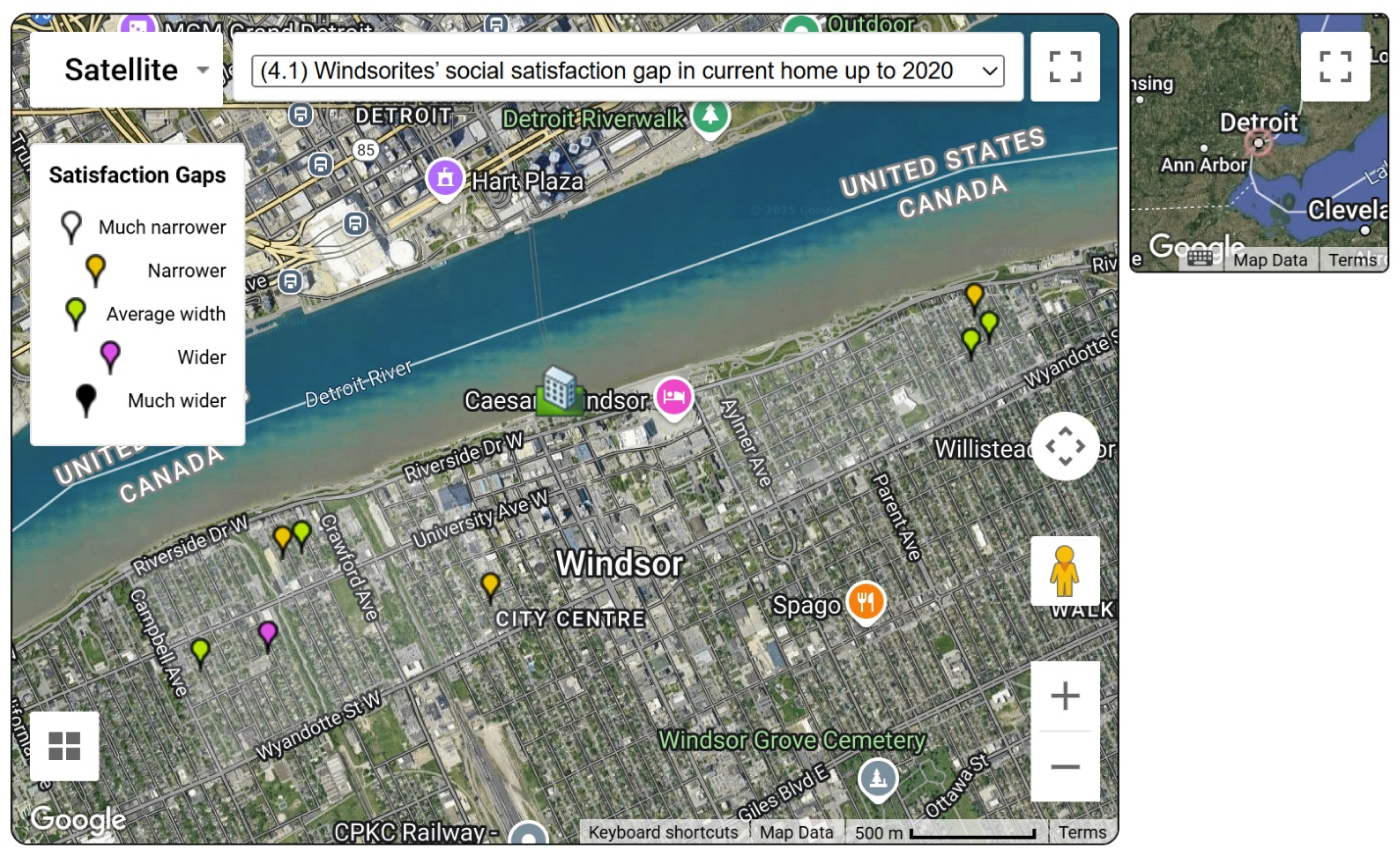
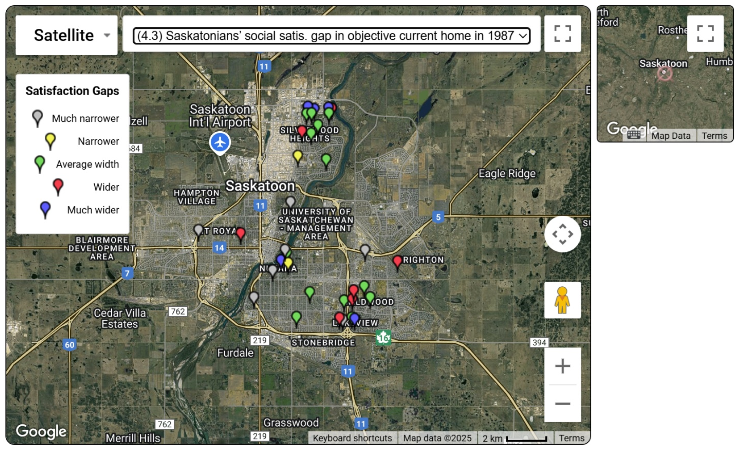
In fact, despite the narrow average overall satisfaction gaps predicted for them, no Windsorites and very few Saskatonians would have 0% social or economic satisfaction gaps in their current home OAs or SAs. Up to four Windsorites’ homes at one time of sale or another would have not-zero narrower social or economic satisfaction gaps than 10% and 7% or approximately one standard deviation below the respective mean percentage; one would have both types of gaps (Figure 1 and option 4.1 of the online figure on https://alanorpaulinephipps.ca/courses/np/gwcmaps.html (accessed on 19 July 2026). Less than one-fifth of Saskatonians would have no social or economic satisfaction gaps in current home OAs, and less than one-tenth in current home SAs. Their homes were in the urban core of the city in 1987, alongside those with narrow social satisfaction gaps of less than 5% or one standard deviation below the mean percentage (Figure 2 and option 4.3 in the online figure). Note that the maps locate the respondents’ current homes and classify the widths of their social or economic satisfaction gaps as much narrower than average, narrower than average, average, wider than average or much wider than average with the overall histogram percentage scale in Table 2.
Conversely, less than one-third of Saskatonians and Windsorites had current homes with OAs producing wider or much wider social satisfaction gaps than 30% and 20% or minus- and plus-one standard deviation of their respective mean percentage (Table 2). Behind the scenes, these dissatisfactory current homes tended to have above-average sale or asking prices. Their resident respondents may have been stressed owner occupiers, as they likely were younger than 36 or 41 years old and had above-average search price ranges but also lower incomes than average during the past 12 months, at least in Saskatoon. These Saskatonians’ current homes were in the city’s new northern and eastern suburbs outside the urban core in 1987. Correspondingly, their gappy OAs in these homes would be the peripheral accessibility and underdeveloped environment and expensiveness of new suburban homes in the 1980s, from social and economic points of view, respectively [16,18,20]. Supplementing this, Windsorites’ wider than average social and economic satisfaction gaps might also be present partly due to their inner city neighbourhood’s overgrown landscaping in need of replanting or pruning, and their presumably older home’s unfinished basement condition and timeworn renovations, mirroring contemporary findings in inner city Brisbane, Australia [21].

6. Conclusions

Three distinct conceptualizations of the causes of residential (dis-)satisfaction with a home have been synthesized in a utility modelling framework. This theoretical framework has translated a resident’s feelings about the attributes of a home into a social or economic satisfaction gap between their most preferred levels of those attributes and their experienced ones. A wide social satisfaction gap is predicted when home attributes have less usefulness for residents than they would prefer and can afford. An alternative economic satisfaction gap will be wide for possibly different attributes whose prices are not the highest that they would be willing to pay for. The study’s conclusion bolstered by tentative substantive findings from small samples of residents, such as new suburban homes and older inner city ones creating akin yet distinct social or economic satisfaction gaps over time, concerns its four theoretical and practical contributions.
The first theoretical and practical contribution of this experimental study is the demonstration that a resident’s satisfaction with a home was predictable with a utility modelling framework. The majority of respondents were predicted to be satisfied socially and economically with their current homes—which is not surprising as many had recently moved into them. However, respondents’ social and economic satisfaction gaps in terms of attributes of the dwelling unit, its accessibility, and its neighbourhood landscaping were also predicted to reoccur over time, beginning with those in expensive new homes in inaccessible suburbs in 1987 and ending with those in deteriorating older homes in ‘inaccessible’ inner city neighbourhoods in 2020.
Second, similar predictions were derived from a resident’s utilities and prices of their SAs or their OAs coded from an MLS listing and neighbourhood census data, though with possible exceptions of subjectively better home accessibilities. These similar predictions should enable the prediction of a resident’s satisfaction with a home that they cannot directly evaluate until they have experience of it, such as a prospective new home. These predictions would be especially useful prior to travelling distances for personal inspections.
Third, the calculated satisfaction gaps in each of the SAs or OAs of a home represented the sources of a resident’s overall (dis-)satisfaction with that home. A resident or a policymaker will surely be interested in knowing which attributes require adjustment for improved residential satisfaction. They will necessarily prefer a quantified magnitude of the social or economic satisfaction gap in a home for predicting the amount of an improvement. They will likely seek more than a simple classification as in other studies of whether a resident has a social or economic satisfaction gap or not. Our speculative calculations of attributes’ gaps for three published studies provide a method of calculating such gaps in interval-scaled levels, which has enabled comparisons between at least two important attributes of dwelling size and distance to stores despite the small samples in this study.
Fourth, respondents’ social (dis-)satisfaction with some attributes of a home over time, such as those of their dwelling unit, complemented their economic (dis-)satisfaction with them—but not with others, such as their neighbours’ ages and neighbourhood landscaping. Resolving a social satisfaction gap in a home would require different attribute adjustments depending on whether an economic satisfaction gap is also present, and vice versa. For sure, a surveyed satisfaction gap between a home’s experienced attributes and a resident’s most preferred ones should always be open to interpretation from a social or an economic point of view.
In the final analysis, these conclusions are limited by the small samples of respondents whose home’s objective attributes were coded from among hundreds of sold or for sale homes. Current homes of one-half of Saskatoon respondents had both SAs and OAs, while fewer current homes of Windsor respondents had OAs. These OAs are required for this study’s contribution to reducing the subjective data requirements of potential respondents for predicting their residential satisfaction gaps. However, the coding of OAs, especially of movers’ new homes and thinking movers’ current homes, will be even more arduous for future research. Fewer homeowner residents, especially identified as movers or thinking movers, seem to participate in an online surveying experiment nowadays than those who participated in the simulation game previously. Homes’ OAs are measured for particular residents and so are their social utilities too but, in the future, they may be generalized with new information technologies for predicting similar residents’ residential satisfaction gaps with this study’s utility modelling framework.

Author Contributions

Conceptualization, A.G.P. and W.J.; methodology, A.G.P. and W.J.; formal analysis, A.G.P.; investigation, A.G.P. and W.J.; data curation, A.G.P.; writing—original draft preparation, A.G.P. and W.J.; writing—review and editing, W.J. All authors have read and agreed to the published version of the manuscript.

Funding

This research received no external funding.

Institutional Review Board Statement

This study was conducted in accordance with the Declaration of Helsinki. The University of Windsor Research Ethics Board approved the online conjoint choice experiment reported in this study on 16 January 2018, protocol code REB#19-017. The title of the project was the Glengarry and Wellington-Crawford Geographical Monitoring Project: Housing Surveys. The final report for the project was submitted on 17 August 2022: it states that no ethical concerns arose in the course of the research. Research ethics review was not instituted at the time of the corresponding conjoint choice experiment in Saskatoon in 1987.

Informed Consent Statement

Informed consent was obtained from all subjects involved in the study.

Data Availability Statement

The social utility data of 70 anonymous respondents in the human–computer simulation game in Saskatoon, SK, in 1987, and 74 anonymous respondents in the online surveying project in Windsor, ON, in 2020, as well as the latter’s house price data are freely available in the Borealis dataverse of the consortium of Canadian universities at the respective links: https://doi.org/10.5683/SP3/PDS5UV, https://doi.org/10.5683/SP3/3HGFRP, and https://doi.org/10.5683/SP2/ZYXHZ4.

Conflicts of Interest

The authors declare no conflicts of interest.

Abbreviations

The following abbreviations are used in this manuscript:
BCBudget-constrained
CTCensus tract
DADissemination area
MLSMultiple Listing Service
OAObjective attribute
SASubjective attribute
UCUnconstrained

References

  1. Terzano, K. Residential satisfaction. In Encyclopedia of Quality of Life and Well-Being Research, 2nd ed.; Maggino, F., Ed.; Springer: Cham, Switzerland, 2023; pp. 5970–5972. [Google Scholar]
  2. Smith, K.; Cohen, L.; Pooley, J.A. Residential Satisfaction, Sense of Community, Belonging and Place: Residential Satisfaction in a Planned Community; LAP LAMBERT Academic Publishing: Saarbrücken, Germany, 2012. [Google Scholar]
  3. Francescato, G.; Weidemann, S.; Anderson, J.R. Chapter 7 Evaluating the built environment from the users’ perspective: Implications of attitudinal models of satisfaction. In Building Performance Evaluation: From Delivery Process to Life Cycle Phases; Preiser, W.F., Hardy, A.E., Schramm, U., Eds.; Springer: Cham, Switzerland, 2018; pp. 87–97. [Google Scholar] [CrossRef] [Scilit]
  4. Emami, A.; Sadeghlou, S. Residential satisfaction: A narrative literature review towards identification of core determinants and indicators. Hous. Theory Soc. 2021, 38, 512–540. [Google Scholar] [CrossRef] [Scilit]
  5. Mridha, M. Looking through the models: A critical review of residential satisfaction. Buildings 2023, 13, 1183. [Google Scholar] [CrossRef] [Scilit]
  6. Aigbavboa, C.; Thwala, W. Residential Satisfaction and Housing Policy Evolution, 1st ed.; Routledge Studies in International Real Estate: Abingdon, UK, 2018. [Google Scholar]
  7. Jansen, S.J.T. The impact of the have-want discrepancy on residential satisfaction. J. Environ. Psychol. 2014, 40, 26–38. [Google Scholar] [CrossRef] [Scilit]
  8. Xu, S.; Chen, M.; Yuan, B.; Zhou, Y.; Zhang, J. Resident satisfaction and influencing factors of the renewal of old communities. J. Urban Plan. Dev. 2023, 150, 1. [Google Scholar] [CrossRef] [Scilit]
  9. Smrke, U.; Blenkuš, M.; Sočan, G. Residential satisfaction questionnaires: A systematic review. Urbani Izziv 2018, 29, 67–82. [Google Scholar] [CrossRef] [Scilit]
  10. Amole, D. Residential satisfaction in students’ housing. J. Environ. Psychol. 2009, 29, 76–85. [Google Scholar] [CrossRef] [Scilit]
  11. Galster, G. Identifying the correlates of dwelling satisfaction: An empirical critique. Environ. Behav. 1987, 19, 539–568. [Google Scholar] [CrossRef] [Scilit]
  12. Liu, Y.; Shakib, S.; Higgins, C.D.; Farber, S.; Miller, E.J.; Habib, K.N. What drives you to relocate your home? Investigating preferences and residential mismatching of recent (prior to COVID and during-after COVID) movers in the Greater Toronto Area. Environ. Plan. B Urban Anal. City Sci. 2025. [Google Scholar] [CrossRef] [Scilit]
  13. Ryan-Collins, J.; Lloyd, T.; Macfarlane, L. Rethinking the Economics of Land and Housing; Zed Books, Bloomsbury Publishing Plc: London, UK, 2017. [Google Scholar]
  14. Amérigo, M.; Aragonés, J.I. A theoretical and methodological approach to the study of residential satisfaction. J. Environ. Psychol. 1997, 17, 47–57. [Google Scholar] [CrossRef] [Scilit]
  15. Crawford, J.; McKee, K. Hysteresis: Understanding the housing aspirations gap. Sociology 2018, 52, 182–197. [Google Scholar] [CrossRef] [Scilit]
  16. Cutter, S.L. Residential satisfaction and the suburban homeowner. Urban Geogr. 1982, 3, 315–327. [Google Scholar] [CrossRef] [Scilit]
  17. Ley, D. Alternative explanations for inner-city gentrification: A Canadian assessment. Ann. Assoc. Am. Geogr. 1986, 76, 521–535. [Google Scholar] [CrossRef] [Scilit]
  18. Brower, S. Good Neighborhoods: A Study of In-Town and Suburban Residential Environments; Praeger: Westport, CT, USA, 1996. [Google Scholar]
  19. Day, R.A.; Walmsley, D.J. Residential preferences in Sydney’s inner suburbs: A study in diversity. Appl. Geogr. 1981, 1, 185–197. [Google Scholar] [CrossRef] [Scilit]
  20. Rothblatt, D.N.; Garr, D.J. Suburbia: An international perspective on levels of satisfaction with the physical environment. J. Plan. Educ. Res. 1986, 5, 94–106. [Google Scholar] [CrossRef] [Scilit]
  21. Buys, L.; Miller, E. Residential satisfaction in inner urban higher-density Brisbane, Australia: Role of dwelling design, neighbourhood and neighbours. J. Environ. Plan. Manag. 2012, 55, 319–338. [Google Scholar] [CrossRef] [Scilit]
  22. McCrea, R.; Shyy, T.-K.; Stimson, R.J. Satisfied residents in different types of local areas: Measuring what’s most important. Soc. Indic. Res. 2014, 118, 87–101. [Google Scholar] [CrossRef] [Scilit]
  23. Alemu, L.S.; Berhanu, W.; Sokkido, D.L. Determinants of residential satisfaction: An actual-aspiration gap theory analysis in low-cost condominium housing, Addis Ababa, Ethiopia. Urban Plan. Transp. Res. 2025, 13, 2475960. [Google Scholar] [CrossRef] [Scilit]
  24. Davoodi, T.; Yapicioglu, B.; Dağlı, U.U. Measuring residential satisfaction in historic areas using actual–aspiration gap theory: The case of Famagusta, Northern Cyprus. Sustainability 2023, 15, 3917. [Google Scholar] [CrossRef] [Scilit]
  25. Hou, H.C.; Lai, J.H.K.; Edwards, D. Gap theory based post-occupancy evaluation (GTbPOE) of dormitory building performance: A case study and a comparative analysis. Build. Environ. 2020, 185, 107312. [Google Scholar] [CrossRef] [Scilit] [PubMed]
  26. Jiang, W.; Timmermans, H.J.P. Residential satisfaction in renovated historic blocks in two Chinese cities. Prof. Geogr. 2021, 73, 333–347. [Google Scholar] [CrossRef] [Scilit]
  27. Jiang, W.; Feng, T.; Timmermans, H.J.P. Non-linear asymmetric gap models of residential satisfaction: Formulation and empirical evidence. Environ. Plan. B Urban Anal. City Sci. 2020, 47, 569–589. [Google Scholar] [CrossRef] [Scilit]
  28. Jiang, W.; Feng, T.; Timmermans, H.J.P.; Li, H. A gap-theoretical path model of residential satisfaction and intention to move house applied to renovated historical blocks in two Chinese cities. Cities 2017, 71, 19–29. [Google Scholar] [CrossRef] [Scilit]
  29. Phyu, P.E.; Effendi, N.; Purnawan, P. Assessment of residential satisfaction using gap analysis: A case study in Naypyitaw City, Myanmar. J. Tek. Sipil 2024, 20, 176–190. [Google Scholar] [CrossRef] [Scilit]
  30. Septayuda, A.; Yossyafra, Y.; Hidayat, B. Residential satisfaction analysis of developer products. Int. J. Politics Sociol. Res. 2022, 10, 136–144. Available online: https://ijobsor.pelnus.ac.id/index.php/ijopsor/article/view/62 (accessed on 19 July 2026).
  31. Yan, J.; Bao, H.X.H. A prospect theory-based analysis of housing satisfaction with relocations: Field evidence from China. Cities 2018, 83, 193–202. [Google Scholar] [CrossRef] [Scilit]
  32. Wolday, F.; Böcker, I. Exploring changes in residential preference during COVID-19: Implications to contemporary urban planning. Environ. Plan. B Urban Anal. City Sci. 2023, 50, 1280–1297. [Google Scholar] [CrossRef] [Scilit] [PubMed]
  33. Handal, P.J.; Barling, P.W.; Morrissy, E. Development of perceived and preferred measures of physical and social characteristics of the residential environment and their relationship to satisfaction. J. Community Psychol. 1981, 9, 118–124. [Google Scholar] [CrossRef] [Scilit]
  34. Wang, Y.; Wang, D.; Wang, F.; Sanwei, H.; Wang, L. Does have-want discrepancy or have-had discrepancy explain residential satisfaction? A study of migrant workers in Wuhan, China. Cities 2024, 145, 104708. [Google Scholar] [CrossRef] [Scilit]
  35. Amérigo, M.; Aragonés, J.I. Residential satisfaction in council housing. J. Environ. Psychol. 1990, 10, 313–325. [Google Scholar] [CrossRef] [Scilit]
  36. Pagani, A.; Fritz, L.; Hansmann, R.; Kaufmann, V.; Binder, C.R. How the first wave of COVID-19 in Switzerland affected residential preferences. Cities Health 2021, 7, 602–614. [Google Scholar] [CrossRef] [Scilit]
  37. Carifio, J.; Perla, R. Resolving the 50-year debate around using and misusing Likert scales. Med. Educ. 2008, 42, 1150–1152. [Google Scholar] [CrossRef] [Scilit] [PubMed]
  38. Joshi, A.; Kale, S.; Chandel, S.; Pal, D.K. Likert Scale: Explored and explained. Br. J. Appl. Sci. Technol. 2015, 7, 396–403. [Google Scholar] [CrossRef] [Scilit]
  39. Fishburn, P.C. Utility Theory for Decision Making; Wiley: New York, NY, USA, 1970. [Google Scholar]
  40. Phipps, A.G. Housing Unaffordability from a Resident’s Point of View; Cambridge Scholars Publishing: Newcastle, UK, 2023. [Google Scholar]
  41. Shefer, D. Utility changes in housing and neighborhood services for households moving into and out of distressed neighborhoods. J. Urban Econ. 1986, 19, 107–124. [Google Scholar] [CrossRef] [Scilit]
  42. Deurloo, M.C.; Dieleman, F.M.; Clark, W.A.V. Generalized log-linear models of housing choice. Environ. Plan. A 1988, 20, 55–69. [Google Scholar] [CrossRef] [Scilit]
  43. Short, J.R. Residential mobility. Prog. Hum. Geogr. 1978, 2, 419–447. [Google Scholar] [CrossRef] [Scilit]
  44. Boumeester, H.J.F.M. Traditional housing demand research. In The Measurement and Analysis of Housing Preference and Choice; Jansen, S.J.T., Coolen, H.C., Goetgeluk, R.W., Eds.; Springer: Berlin, Germany, 2011; pp. 27–55. [Google Scholar]
  45. Kabisch, S.; Poessneck, J.; Soeding, M.; Schlink, U. Measuring residential satisfaction over time: Results from a unique long-term study of a large housing estate. Hous. Stud. 2021, 37, 1858–1876. [Google Scholar] [CrossRef] [Scilit]
  46. Boschman, S. Individual differences in the neighbourhood level determinants of residential satisfaction. Hous. Stud. 2018, 33, 1127–1143. [Google Scholar] [CrossRef] [Scilit]
  47. Lovejoy, K.; Handy, S.; Mokhtarian, P. Neighborhood satisfaction in suburban versus traditional environments: An evaluation of contributing characteristics in eight California neighborhoods. Landsc. Urban Plan. 2010, 97, 37–48. [Google Scholar] [CrossRef] [Scilit]
  48. Riazi, M.; Emami, A. Residential satisfaction in affordable housing: A mixed method study. Cities 2018, 82, 1–9. [Google Scholar] [CrossRef] [Scilit]
  49. Rosetta Code. Javascript Multiple Regression. Available online: http://rosettacode.org/wiki/Multiple_regression#JavaScript (accessed on 27 May 2026).
  50. Takane, Y.; Young, F.W.; de Leeuw, J. An individual differences additive model: An alternating least squares method with optimal scaling features. Psychometrika 1980, 45, 183–209. [Google Scholar] [CrossRef] [Scilit]
  51. Statistics Canada. Dictionary Census of Population: Dissemination Area (DA); Government of Canada: Ottawa, ON, Canada, 2017. Available online: https://www12.statcan.gc.ca/census-recensement/2021/ref/dict/az/Definition-eng.cfm?ID=geo021 (accessed on 27 May 2026).
Figure 1. Windsor respondents’ social or economic satisfaction gaps in their current homes.
Urbansci 10 00419 g001
Figure 2. Saskatoon respondents’ social or economic satisfaction gaps in their current homes.
Urbansci 10 00419 g002
Table 1. Windsor experimental and observed home accessibility attributes.
2020 Experimental Attribute and Level1986–2023 Observed House Variable Classes
10. Stores and Work Access0. Within easy driving or walking access, up to 10 min of major stores and/or work.12.0 Distance from downtown (km)2.00
1. Not too far from major stores and/or work, up to 20 min by car or bus.1.25
2. Far from major stores and/or work, at least 30 min by car or bus.0.50
11. School Access0. Within 10 min walking to a school.13.0 Distance from nearest school (km)0.10
1. About 20 min walking or 10 min driving to a school.1.00
2. Up to 25 to 30 min drive or bus ride to a school.2.00
12. Riverbank Access0. On the Detroit riverbank.14.0 Distance from Detroit riverbank (km)0.05
1. About 10 min walking or a few blocks to the Detroit riverbank.1.00
2. Not conveniently close to the Detroit riverbank.2.00
Source: Table created by authors.
Table 2. Residential satisfaction gaps in current homes.
2020 Windsor1987 Saskatoon
Social Satis a Gap Economic Satis Gap Social Satisfaction GapEconomic Satisfaction Gap
in OAs bin OAsin OAsin SAs cin OAsin SAs
Overall StatisticsMean15%11%18%10%3%4%
Standard deviation5%4%13%7%2%2%
Observed minimum8%6%0%0%0%0%
Observed maximum21%16%46%26%7%8%
Overall HistogramNumber of sales or homes for sale d141435343535
Much narrower than average < 5%00772717
Narrower than average 5 ≤ 10%46213818
Average width 10 ≤ 20%78131000
Wider than average 20 ≤ 30%307400
Much wider than average 30–50%006000
Attribute MeansHouse type and size11%10%10%13%7%14%
Home age (and exterior finish) e8%11%15%11%9%9%
Basement condition and home renovations15%26%19%14%6%5%
Lot size (and garage)13%13%15%11%4%4%
Neighbourhood landscaping26%8%28%16%3%2%
Neighbouring housing (and repair)17%5%27%8%5%8%
Neighbours’ ages13%1%31%17%2%1%
Neighbours’ ethnicity and education18%5%8%8%3%8%
Neighbours’ mobility6%4%14%7%1%2%
Stores and work access26%19%42%3%2%0%
School access15%5%29%12%0%0%
Parks (or riverbank) access10%25%18%11%1%1%
Source: Table created by authors. a Satisfaction. b Objective attributes of current homes coded from MLS and national census. c Subjective attributes of current homes elicited from respondents in the simulation game. d Number of sales includes repeated sales of some houses. e Embellishment of a Windsor attribute in parentheses.
Disclaimer/Publisher’s Note: The statements, opinions and data contained in all publications are solely those of the individual author(s) and contributor(s) and not of MDPI and/or the editor(s). MDPI and/or the editor(s) disclaim responsibility for any injury to people or property resulting from any ideas, methods, instructions or products referred to in the content.