Assessing Urban Water Balance Dynamics: A Hydrological Modelling Approach Incorporating Vegetation-Impervious Surface-Soil (V-I-S) Fractions

Abstract

Vegetation-impervious surface-soil (V-I-S) fractions offer a continuous sub-pixel representation of urban surface heterogeneity. In this study, the influence of urban surface characteristics represented through V-I-S fractions on hydrological processes is analyzed at decadal intervals, i.e., 2000, 2010, 2020, and the projected year 2030 for the Mula–Mutha river catchment, Maharashtra, India. Pune city, as a major urban centre in this region, is experiencing significant changes in land surface characteristics over time, which have direct implications for its hydrology. The analysis uses the Soil and Water Assessment Tool (SWAT) to model these changes and their effects on water resources. Results show that the urban area has increased from 14% (2000) to 25% (2020), with projections indicating a further rise to 34% (2030). Such transitions yielded an increase in surface runoff from 47% (2000) to 53% (2020) and projected to reach 54% (2030). Groundwater recharge has declined from 10% to 6% and is expected to fall to 4% by 2030. Model validation using discharge data at Mirawadi outlet yielded a coefficient of determination of 0.72 using land use/land cover (LULC) data and 0.79 for simulations based on runoff Curve Number (CN) derived from V-I-S fractions, indicating the improved model performance. This study presents a novel framework, which incorporates remote sensing-derived V-I-S fractions to assess the spatiotemporal impact of urban expansion on water balance components.

1. Introduction

In rapidly growing cities, traditional water management systems such as open drains, tanks, and natural drainage channels are increasingly encroached upon and degraded due to urban expansion, driven by both outward sprawl and redevelopment of existing urban areas [1,2]. The resultant urban growth disrupts the natural water cycle by reducing infiltration, enhancing surface runoff, and accelerating the depletion of groundwater reserves, thereby increasing the vulnerability of the urban population to both drought and flooding. The freshwater sustainability is increasingly threatened by the convergence of human-induced pressure and climate-driven stressors [3]. The effects of climate change on hydrological behaviour are expected to intensify precipitation variability and evapotranspiration losses. The decrease in rainfall may lessen the stormwater impact in certain areas, but it can also create a significant obstacle for water availability and recharge [4,5]. Thus, understanding the urban water balance is vital for guiding proactive planning under changing climate and land use conditions.

The urban water balance represents the distribution of water among its major components, such as precipitation, surface runoff, infiltration, evapotranspiration, soil moisture, and lateral flow, and serves as a vital indicator for understanding hydrological responses to urbanization and climate change. The newly urbanized areas experience significant changes in water balance components due to uncontrolled land use changes and the spread of impervious surfaces. The loss of pervious surfaces and landscape fragmentation leads to decreased soil moisture retention and infiltration capacity, which can increase the risk of flash floods and groundwater stress [6,7].

Hydrological models are useful to predict water flows and balances over a wide range of landscapes, including urban landscapes. Among them, the process-based models like the Soil and Water Assessment Tool (SWAT) have been found to satisfactorily simulate hydrological responses to land use and climate variability. SWAT is a physically based, semi-distributed model that simulates surface processes by incorporating key watershed attributes such as land use, soil type, topography, and meteorological inputs [8,9]. Even though the SWAT model is a physically based and robust tool, its use in urban watershed environments typically requires modifications such as the incorporation of high-resolution impervious surface cover information and detailed Curve Number (CN) estimates to portray the complexity of urban hydrological processes. In particular, the vegetation-impervious surface-soil (V-I-S) fraction datasets offer high-resolution information on surface composition that is especially suited to urban areas. The integration of V-I-S fractions into a hydrological modelling framework allows for the estimation of composite CN that reflects the mixed nature of urban land parcels, thereby improving the realism of surface runoff estimates [10,11]. Several studies have demonstrated the potential of V-I-S-based modelling to enhance flood risk assessment and runoff prediction in urban environments [12,13,14]. However, despite these advances, there is limited understanding of how the V-I-S integrated modelling framework performs at long temporal scales or under scenarios of projected urban expansion.

Moreover, previous investigations have often focused exclusively on either land use change or climatic influences, leaving a critical gap in our understanding of how these two drivers together interact to shape urban water balance dynamics. This gap is particularly evident in Indian cities, where the intersection of rapid urban expansion and increasing climate extremes necessitates a more comprehensive modelling approach that captures both present and future hydrological behaviour. There is a pressing need to quantify how different components of the urban water balance respond to urbanization and changing climate conditions over time.

To address these challenges, this study applies an integrated modelling framework that combines high-resolution satellite data-derived V-I-S fractions, composite CN, and LULC data within the SWAT model to simulate long-term changes in water balance components of the Mula–Mutha river catchment (MMRC) in Maharashtra, India. MMRC has witnessed significant urban expansion in recent decades and provides a representative case for analyzing hydrological responses to urban land surface transformation. The study evaluates hydrological components for four times, viz., 2000, 2010, 2020, and 2030, to trace the trajectory of water balance shifts under progressive urbanization.

2. Study Area

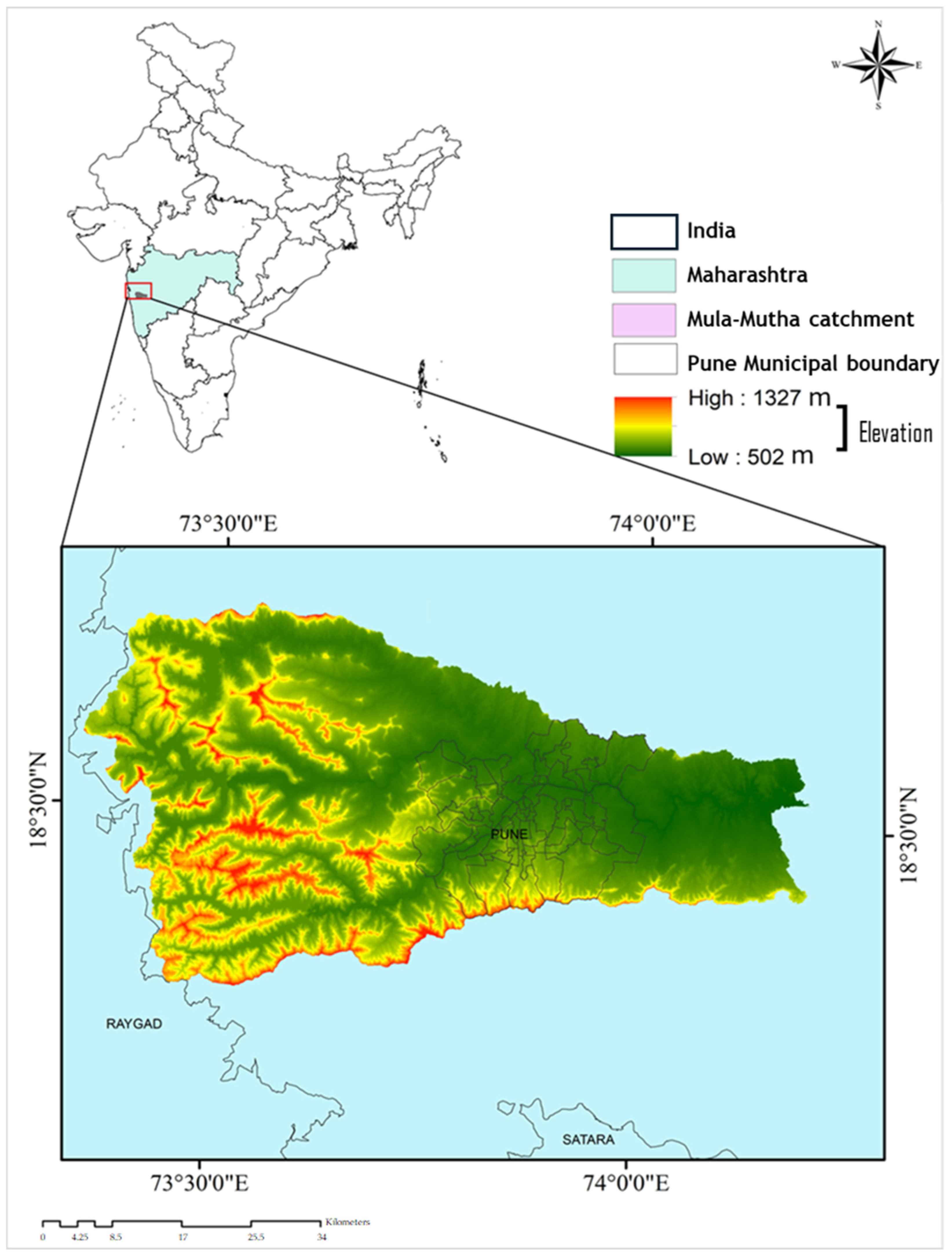
The present study was conducted for the Mula–Mutha river catchment (MMRC), located in West-central India, with its outlet at Mirawadi in the state of Maharashtra. The mean geographic coordinates (centroid) of MMRC are 18°31′50″ N and 73°51′37″ E (Figure 1), with a catchment area of 2638 km². Pune city comprises a major portion of this catchment. The city is located at the confluence of the Mula and Mutha rivers, along the western margin of the Deccan Plateau, and is surrounded by the Sahyadri mountain range. The administrative region includes Pune and Pimpri Chinchwad cities, forming part of the larger Pune district, which occupies around 15,643 km². Pune’s physiography is diverse, transitioning from gentle rolling valleys and flat plains in the eastern sector to rugged hills in the west. This variability plays a significant role in the spatial distribution of runoff and hydrological responses across the basin. The region experiences a tropical climate typical of Maharashtra (India), marked by hot summer, a distinct monsoon season, and mild winters. Summers extend from March to June, with daytime temperatures often reaching 35 to 40 degrees Celsius and very limited precipitation. The southwest monsoon, active from June to September, contributes most of the annual rainfall, which averages approximately 722 mm. Based on India Meteorological Department (IMD) records from 2000 to 2020, annual rainfall in the region exhibits substantial inter-annual variability, ranging from a minimum of 316 mm (2003) to a maximum of 7269 mm (2005). The post-monsoon season brings transitional weather, while winters from December to February are dry and relatively cool with daytime temperatures between 12 and 30 degrees Celsius [15]. The watershed contains a range of soil types, including mixed, brown, and black fertile soils. The western part of the catchment is characterized by darker, less fertile soils with limited water retention, while the eastern plains are more productive and conducive to infiltration. Rich alluvial soils are found particularly in the eastern part of the catchment, especially within the Bhima sub-basin downstream of Mula–Mutha confluence. The vegetation in urban areas includes urban green spaces and protected areas such as Sambhaji Park and Vetal Hill, which serve as important ecological zones and help regulate urban microclimate [16]. Pune city has a population of approximately three million. In the Pune Municipal Corporation area, the urban area has expanded from 18.3 km² in 1973 to 139.4 km² in 2013, representing a nearly 7.5 times increase over four decades, with a mean annual development rate of approximately 3 km² [17]. Its rapid urban growth, driven by industrial and economic development, has significantly influenced the land use pattern and has also altered hydrological processes [18]. Increasing urbanization has resulted in greater surface runoff and reduced evapotranspiration within the Mula and Mutha River catchments [15,19].

The rapid expansion has been accompanied by a substantial increase in impervious surfaces such as concrete roads, rooftops, and paved areas. These surfaces hinder infiltration and accelerate the movement of runoff, reducing water losses through evaporation and infiltration due to shorter contact duration. As a result, the basin exhibits higher vulnerability to flash floods, especially during intense monsoonal precipitation events. The interplay between land use change and altered hydrological behaviour necessitates a detailed assessment using integrated modelling approaches to understand the dynamics of surface runoff and flood risks in this rapidly urbanizing catchment.

3. Materials and Methods

The present study utilizes a range of spatial and climatic datasets from various sources. Digital Elevation Model (DEM) data from the Shuttle Radar Topography Mission (SRTM) with a spatial resolution of 30 m was downloaded from the Earth Resources Observation and Science (EROS) Centre, United States Geological Survey (USGS) website. For land use/land cover (LULC) classification, Landsat 5 TM and Landsat 8 OLI/TIRS satellite images, each having a spatial resolution of 30 m, were downloaded from the USGS Earth Explorer platform. To ensure temporal consistency and minimize seasonal variation, images of the first week of February were selected for the years 2000, 2010, and 2020. Soil characteristics were incorporated from SoilGrids, which offers global soil data at a spatial resolution of 250 m. Precipitation data with a resolution of 0.25° × 0.25°, and minimum and maximum temperature data with a resolution of 1° × 1° were sourced from the India Meteorological Department (IMD) and downscaled Coupled Model Intercomparison Project Phase 6 (CMIP6) is obtained from Google Earth Engine (GEE) with a resolution of 0.25° × 0.25°. Wind speed, solar radiance, and relative humidity were obtained from SWAT-compatible weather generator datasets from the SWAT database [20,21]. Additional spatial data, including road network and building footprints, were obtained from OpenStreetMap (OSM), while water body delineation was performed using a freely available remote sensing dataset. PlanetScope imagery with 3 m resolution was used to produce V-I-S fractions, from which composite curve numbers were then derived (see Section 3.2 for more information).

3.1. Preparation of LULC

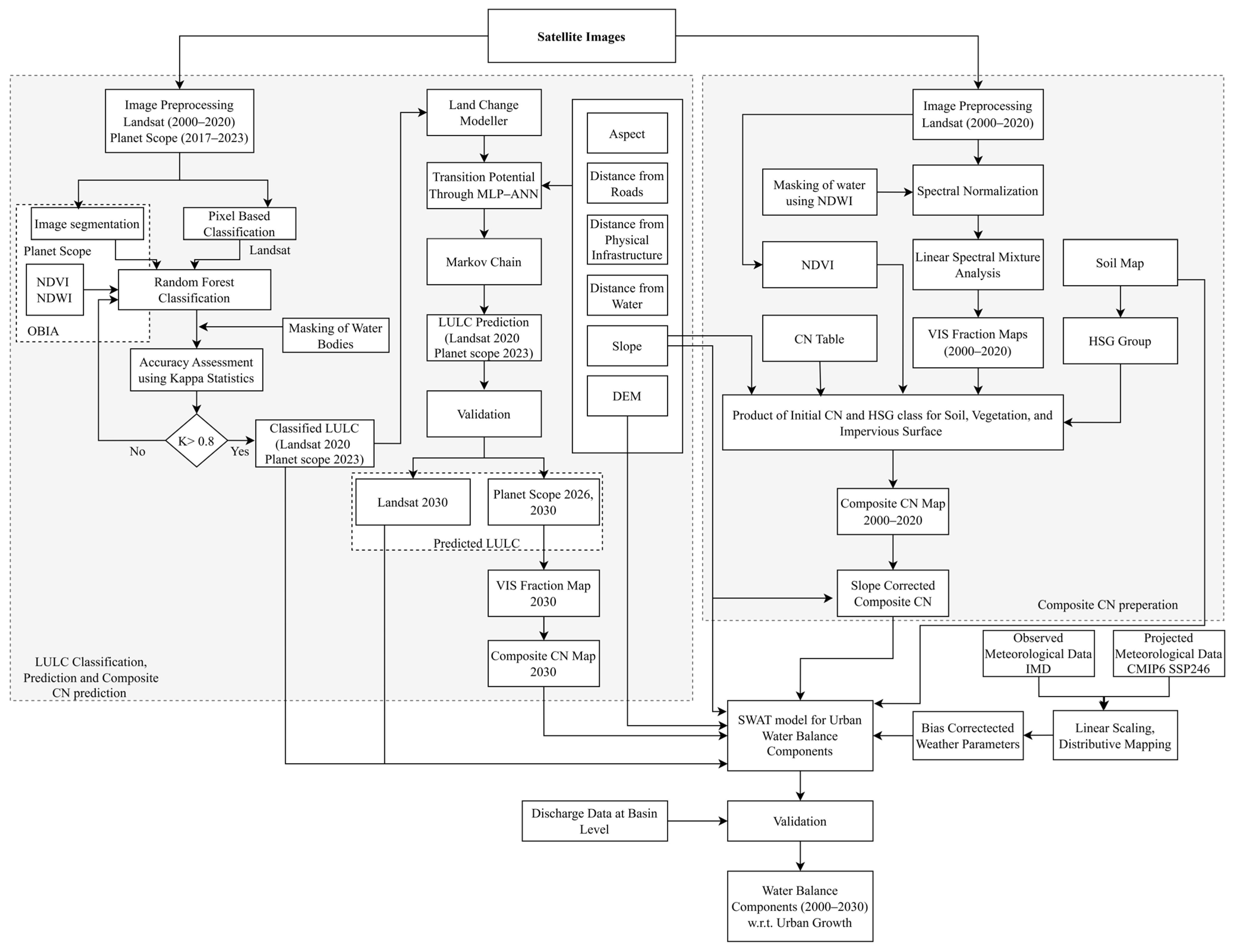
The satellite imagery utilized in this study comprised Landsat 5 and Landsat 8 images for the years 2000, 2010, and 2020 (Figure 2). These were employed for LULC mapping using the GEE platform. Imagery corresponding to specific temporal windows over the MMRC was selected, ensuring minimal cloud cover for optimal classification accuracy. Preprocessing steps involved the extraction of essential spectral bands necessary for effective land cover classification. Random sampling was conducted to generate representative datasets for major LULC classes, namely urban, fallow land, water, forest, and vegetation, based on pure pixels. To ensure statistical robustness, the dataset was stratified and split into training and validation sets in a 70:30 ratio, following the approach of [22]. A Random Forest (RF) classifier was applied with optimized parameters, such as the number of decision trees and variables per node, trained using the designated training dataset [23,24]. The trained model was then used to classify the full extent of the imagery, and a variable importance analysis was conducted to identify the relative contribution of individual spectral bands to classification performance [25]. Model accuracy was evaluated using standard performance metrics, including the confusion matrix, overall classification accuracy, and the Kappa coefficient, all computed within the GEE environment [26,27]. The overall accuracy (OA) was computed as:

$$\mathrm{O}\mathrm{A}={\displaystyle \frac{{\sum }_{\mathrm{i}=1}^{\mathrm{k}}\mathrm{n}\mathrm{i}\mathrm{i}}{\mathrm{N}}}$$

(1)

where nii is the number of correctly classified samples for class i, and N is the total number of samples.

Kappa coefficient (k), which accounts for the possibility of agreement occurring by chance, was computed as

$$\mathrm{k}={\displaystyle \frac{{\mathrm{P}}_0-{\mathrm{P}}_{\mathrm{e}}}{1-{\mathrm{P}}_{\mathrm{e}}}}$$

(2)

where P₀ is the observed accuracy, and P is the expected agreement by chance, derived from marginal totals of the confusion matrix. The classification performance metrics are discussed in detail in Section 4.1.

Change detection analysis was subsequently performed using post-classification comparison techniques, which are among the most widely used remote sensing-based methods for temporal land cover change assessment. This approach enabled the quantification and spatial identification of LULC transitions across the three study years. Ancillary geospatial datasets, such as DEM, road network, stream, and physical infrastructure, were integrated to improve contextual understanding, especially concerning urban expansion [28]. DEM data supported the generation of topographic derivatives such as slope and aspect maps, while OpenStreetMap (OSM) data was used to delineate buffers around built infrastructure and hydrological features. Urban growth patterns between 2000 and 2010 were analyzed in conjunction with relevant spatial variables within the geographical information system (GIS) environment. Additionally, Markov chain models, which represent stochastic transition processes, were used to forecast the probability of LULC changes in the future [29,30]. The computation of LULC change probabilities followed the formulation described in Equation (1), as detailed by [31].

$${S_{\left(t,t+1\right)}=P}_{ij}\times S_{\left(t\right)}$$

(3)

where S_(t) is the system state at time t, and S_{(t + 1)} is the system state at time t + 1, P_ij is the transition probability matrix in a state that is computed as follows:

$$=‖P_{ij}‖‖\begin{array}{cc}{p}_{\mathrm{1,1}}\dots & p_{1,N}\\ p_{N,1}\dots & p_{N,N}\end{array}‖$$

(4)

P represents the transition probability, P_ij denotes the likelihood of change from the current state, i, to a different state, j, in the future, and P_N is the state probability at any given time. The chance of a low transition is close to (0), whereas that of a high transition is close to 1. Future land cover categories were predicted using the transition probability matrix [32,33]. In particular, land use categories for 2020 were predicted using the matrix for the 2000–2010 period. This forecast was then verified against the 2020 classified LULC data. In the same manner, the land use categories for 2030 were anticipated using the transition probability matrix for the 2010–2020 period.

3.2. Preparation of Composite Curve Number

Using a linear unmixing technique, a fractional impervious surface area map was generated and subsequently normalized to effectively extract features for CN calculation [11]. To minimize variability between pixels representing soil, vegetation, and impervious surfaces, the reflectance values of all spectral bands were initially standardized. This normalization process involved scaling down absolute reflectance values to emphasize shape information rather than magnitude. To further refine the analysis, water pixels were masked using the Normalized Difference Water Index (NDWI) [34]. Following normalization, the linear spectral unmixing was applied, and the necessary endmembers were identified using the Minimum Noise Fraction (MNF) transformation [35].

The normalized inverse MNF image was then used to perform Linear Spectral Mixture Analysis (LSMA) [10], enabling the extraction of precise quantitative information at the sub-pixel level. In LSMA, each pixel’s spectral signature is assumed to be a linear combination of spectral values of distinct land cover types, referred to as endmembers. The LSMA model (Equation (3)) mathematically represents this relationship, as follows:

$${\mathrm{R}}_{\mathrm{i}}={\displaystyle {\sum }_{\mathrm{k}=1}^{\mathrm{n}}}{\mathrm{f}}_{\mathrm{k}}{\mathrm{R}}_{\mathrm{i}\mathrm{k}}+{\mathrm{E}\mathrm{R}}_{\mathrm{i}}$$

(5)

where R_ik is the known spectral reflectance of endmember k within the pixel on band i, f_(k) is the fraction of endmember k within the pixel, and ER_i is the error for band i [36].

The hydrologic soil–cover combination was applied in the V-I-S model to represent three principal urban surface categories: vegetation, impervious surfaces, and soil [37]. Normalized values were used to generate V-I-S fraction maps for three different years, which were then validated using high-resolution Google Earth imagery. To evaluate accuracy, 100 polygons for each class were randomly selected, and the proportions derived from LSMA components [38] were compared with reference data. Next, Normalized Difference Vegetation Index (NDVI), soil classification data obtained from the USDA, and the V-I-S fraction maps were integrated to estimate the composite CN. The calculation considered the proportion of impervious surface area, NDVI values, and soil types. Based on the TR-55 method, an initial CN value was assigned to each soil class, while NDVI thresholds were used to determine CN values for vegetation. Finally, the composite CN was calculated as a weighted average of the impervious surface, vegetation, and soil classes, as represented in Equation (4) [39].

$${CN}_c=I\times {CN}_I+V\times {CN}_V+S\times {CN}_S$$

(6)

The percentages of impermeable surface, vegetation, and soil are represented by I, V, and S in this case; the terms composite CN, initial impervious surface CN, vegetation CN, and soil CN, respectively, are CN_C, CN_I, CN_V, and CN_S.

To forecast future V-I-S (vegetation-impervious surface-soil) maps, the study employed Object-Based Image Analysis (OBIA) as a systematic approach to improve the accuracy of LULC classification [40,41,42]. Using high-resolution (3 m) PlanetScope imagery, LULC classification was performed for the years 2017, 2020, and 2023. Multi-Resolution Segmentation (MRS) was applied to segment the imagery into coherent objects, integrating spectral, spatial, and contextual data for enhanced classification [43]. To further refine the classification, vegetation and water indices such as NDVI and NDWI were incorporated [36]. Supervised classification techniques, including RF and Support Vector Machine (SVM), along with rule-based classification strategies, were used to improve segmentation outcomes and ensure precise LULC mapping. The performance of classification algorithms was rigorously evaluated using confusion and error matrices [44,45]. Additionally, a Markov chain-based predictive modelling technique was employed to project the LULC scenario for the year 2030. Zonal statistics were then used to compute the projected V-I-S fractions by overlaying the predicted 3 m LULC map onto the corresponding 30 m LULC layer.

3.3. Water Balance Modelling

SWAT was utilized to evaluate decadal-scale variations in water balance components (Figure 2). Essential input datasets included classified and projected LULC, a 200 m resolution soil map from the USDA, and slope information derived from DEM. Watershed delineation was carried out using the DEM for a specified outlet point, resulting in the subdivision of the catchment into 240 sub-basins based on a minimum threshold area of 500 hectares [46]. Subsequently, soil, slope, and LULC data were reclassified into hydrologically meaningful units using SWAT’s coding structure to define Hydrologic Response Units (HRUs) [47]. A zero percent threshold was applied to the HRU definition to ensure full spatial representation, thereby including all land cover combinations in the modelling framework [48,49]. Daily meteorological data, including precipitation (mm), maximum and minimum air temperature (°C), were obtained from IMD for the period from 1 January 1950 to 31 December 2021. These datasets were sourced from seven meteorological stations located within the study basin. Supplementary climatic parameters such as solar radiation, wind speed, and relative humidity were acquired from the weather generator database to fill spatial and temporal gaps [50].

Daily precipitation and temperature data were extracted from two Coupled Model Intercomparison Project Phase 6 (CMIP6) global climate models, i.e., Max Planck Institute Earth System Model high resolution (MPI-ESM1.2 HR) and ACCESS CM2, covering the period from 2000 to 2030 for future climate projections. To ensure consistency with observed climatic conditions, bias correction of the climate model outputs was performed using IMD reference datasets under the assumption of bias stationarity [51,52]. This study assessed four bias correction methods: Linear Scaling Method (LSM), Power Transformation (PT), Local Intensity Scaling (LOCI), and Distribution Mapping (DM), to correct biases in precipitation, maximum temperature (T_max), and minimum temperature (T_min) data. Among these, LSM and DM demonstrated the most promising performance, particularly when applied to the outputs of the ACCESS CM2 and MPI ESM 1.2 HR General Circulation Models (GCMs). The performance evaluation of these two GCMs was conducted using key statistical metrics: Mean Absolute Error (MAE), Root Mean Square Error (RMSE), Nash–Sutcliffe Efficiency (NSE), and the coefficient of determination (R²), focusing on precipitation, T_max, and T_min under LSM and DM bias correction approaches [53,54,55,56]. To assess the impact of land use change on runoff generation, eight model scenarios were developed using categorical and V-I-S-based composite CN values for the years 2000, 2010, 2020, and 2030 (see Section 4.3 for details). Once all datasets, including watershed boundary, LULC, slope, soil, and meteorological records, were prepared, SWAT simulations were carried out at a daily temporal resolution for these LULC scenarios. All other input parameters were held constant to isolate the effects of land use change on hydrological response [57]. A warmup period of two years was incorporated, and the model was run from 1998 to 2030 to ensure hydrological stability.

The composite CN values were derived from sub-pixel fractional land cover estimates based on V-I-S analysis (see Section 4.2 for details) and were manually integrated into the CN2 table in the SWAT management file, replacing the default CN values generated by the model using categorical LULC, soil, and slope combinations. This modification enabled more nuanced representation of hydrological responses, particularly in urbanizing regions [14,58,59]. The SWAT model was again executed with the updated CN values. A comparative assessment was conducted to estimate the effect of urban growth on water balance components, including surface runoff, evapotranspiration (ET), and groundwater recharge, in both conventional LULC-based and VIS-based CN model methods.

4. Results and Discussion

4.1. Land Use/Land Cover Analysis

Classified LULC maps for the years 2000, 2010, and 2020 were generated and used for temporal LULC analysis. These maps provide critical insights into historical and recent patterns of land use, enabling the identification of changes in urban areas, vegetation cover, water bodies, and other land use categories. Such spatial information is essential for monitoring urban growth, assessing ecological impacts, and supporting hydrological and environmental modelling. To evaluate the reliability of classified outputs, an accuracy assessment was conducted using the stratified random sampling method. For each classification year, pure pixels for each LULC class were collected, and a 70:30 method was applied for training and validation. The resulting LULC maps delineated five major land use categories across the study region. The classification accuracy for the years 2000, 2010, and 2020 was computed as 92%, 89.5%, and 93%, respectively. Corresponding Kappa statistics were estimated as 0.86 for 2000, 0.81 for 2010, and 0.90 for 2020. These values indicate a satisfactory level to near-perfect agreement between the classified maps and the reference data, which represents ground truth observations, validating the robustness and consistency of the classification approach. The minor dip in accuracy observed in 2010 may be attributed to challenges such as spectral overlap between LULC classes, seasonal image variability, or mixed-pixel effects due to rapid urban expansion. Nevertheless, the consistently high Kappa coefficients confirm that the classifications are statistically reliable and suitable for use in subsequent analyses, including hydrological modelling, landscape dynamics, and policy-relevant land planning applications.

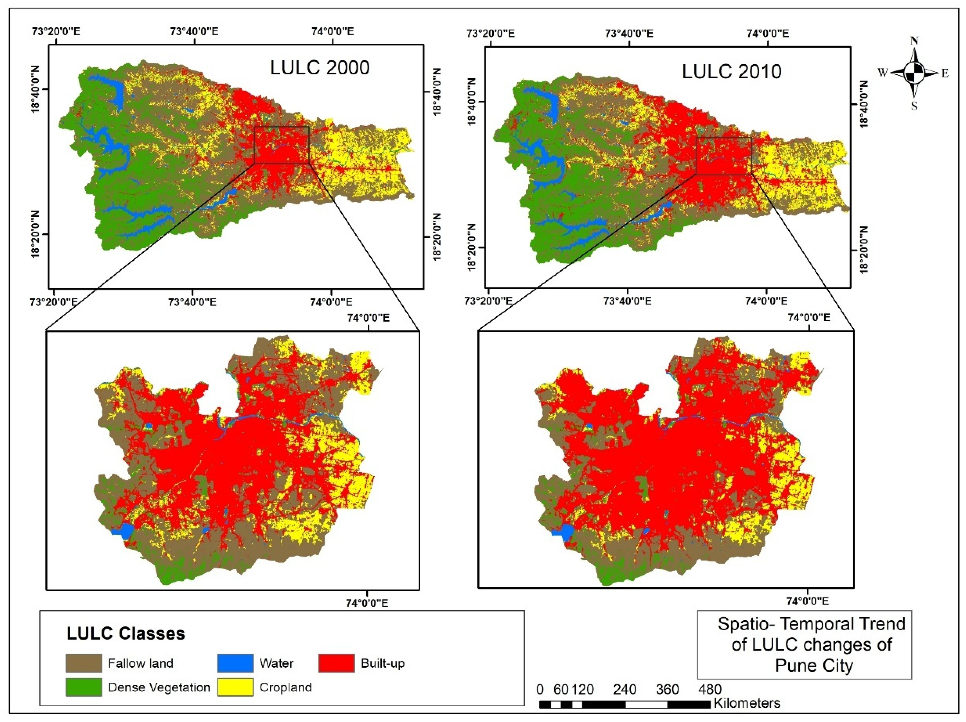
The transition from Scenario 1 (2000) to Scenario 2 (2010) was critically evaluated to forecast LULC changes for the year 2020 using a Markov chain modelling framework. This decadal comparison provides the basis for understanding the spatial and temporal pattern of land transformation and helps anticipate future trends, particularly in fast-growing urban regions. Between 2000 and 2010, the total area under vegetation decreased from 624.58 km² to 617.86 km² (Figure 3). Although this reduction may seem relatively small, it is ecologically significant and suggests ongoing anthropogenic disturbances in natural landscapes. This loss may be attributed to deforestation, encroachment for agriculture, degradation of habitat due to infrastructure development, and urban edge expansion. Even a slight decrease in vegetated areas can result in substantial environmental consequences, including habitat fragmentation, reduced biodiversity, and disruption of ecological functions such as microclimate regulation and soil stability. A more pronounced transformation is observed in the fallow or open space category, which has declined from 1121.22 km² to 992.33 km². This considerable reduction of nearly 129 km² reflects an intensified land utilization pattern. Fallow land typically represents temporarily idle land that may revert to agriculture or convert to built-up areas over time. The declining trend indicates that such lands are increasingly targeted for permanent conversion, often for residential, commercial, or agricultural intensification. This transition suggests a diminishing buffer zone around urban regions, which traditionally absorbs expansion pressure and contributes to the resilience of peri-urban ecosystems.

The most notable and significant change is the expansion of urban sprawl, which grew from 375.68 km² to 529.25 km² during the same period. This increase of approximately 153.57 km² demonstrates the rapid and extensive nature of urban growth in and around the Pune metropolitan area. This expansion is likely driven by multiple factors, including rising population density, increasing demand for housing and infrastructure, industrial development, and enhanced connectivity through transport networks. However, such growth is often unregulated or semi-planned, which can lead to environmental degradation, increasing surface runoff, depletion of natural recharge zones, and deterioration of urban thermal conditions. To project the future LULC distribution, the Markov chain model was employed using transition probabilities derived from the 2000 to 2010 data. Markov chain assumes that land cover in a future time step depends only on the current state and the likelihood of change from one category to another [60,61]. Based on these transition probabilities, a prediction for the year 2020 was generated. The results given as a bar diagram (Supplementary Figure S1) provide a comparative overview of observed and predicted land use distribution.

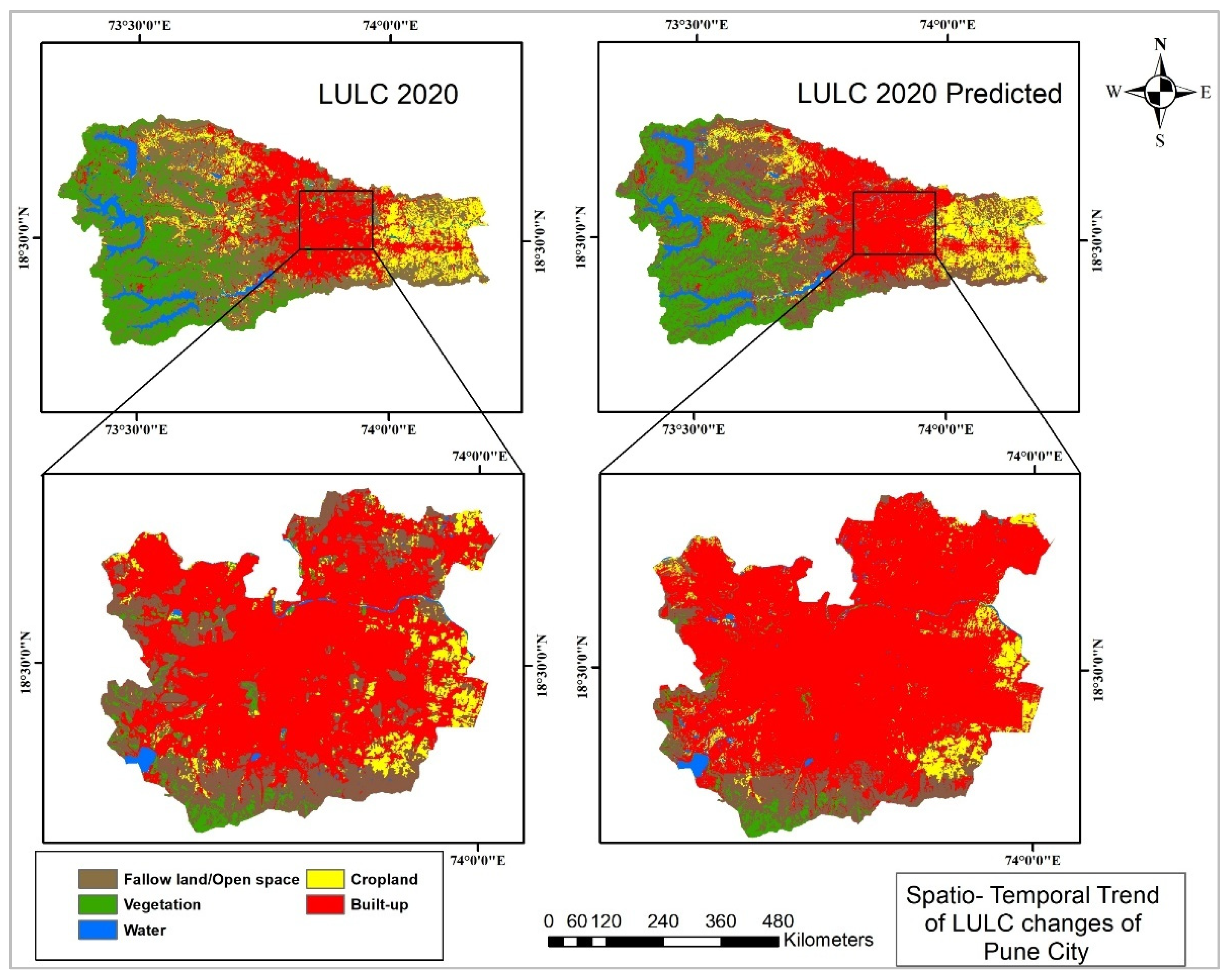
Analysis of the predicted results indicated that the extent of the urban category was overestimated compared to the classified LULC of 2020 (Figure 4, Supplementary Figure S2), while the predicted fallow or open space was underestimated. This divergence indicates that although the model accurately captured the general trend of urban expansion, it slightly over-projected the rate of built-up growth. On the other hand, the lesser predicted extent of fallow land implies that some of the land transition expected by the model may not have occurred due to unforeseen constraints. These constraints may include policy delays, incomplete infrastructure projects, zoning restrictions, socio-economic dynamics, or shifts in land ownership and land use regulation that slowed the pace of conversion. These findings demonstrate the utility and limitations of the Markov chain model in projecting land transformation. While it effectively identifies areas vulnerable to transition and illustrates spatial dynamics of land use change, its predictive accuracy can be enhanced by incorporating socio-political, institutional, and economic variables. Nonetheless, the model serves as a valuable decision-support tool for sustainable urban planning, helping policymakers and planners assess future development scenarios and adopt informed land management strategies.

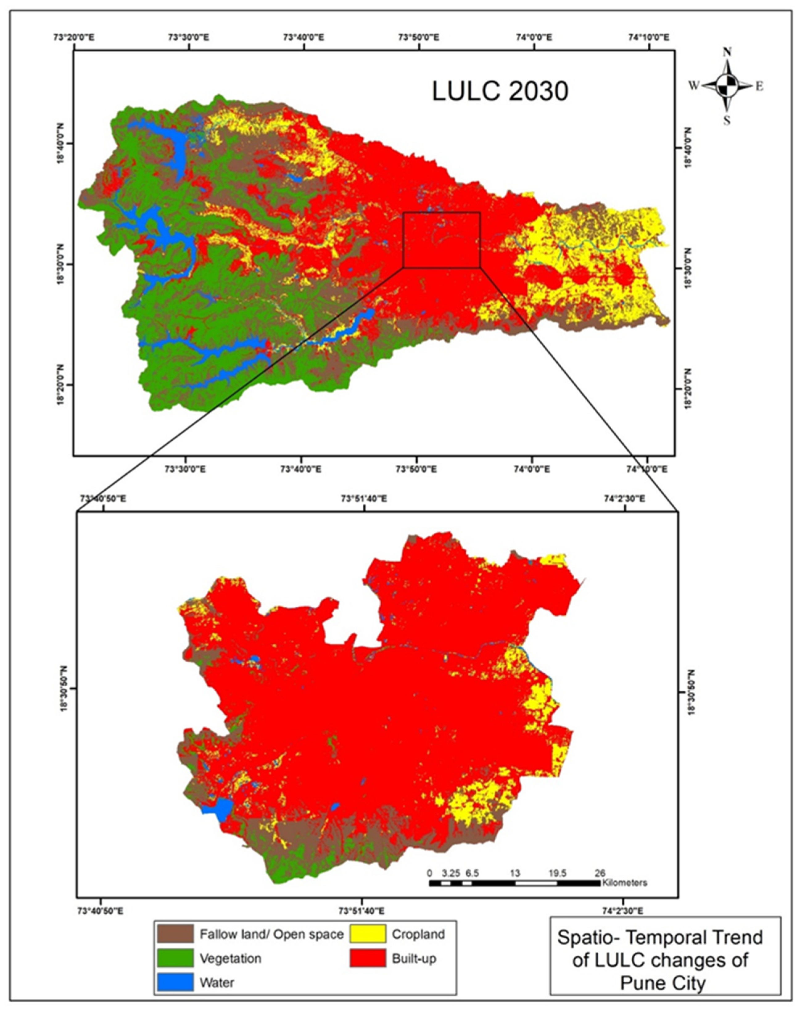
The 2010 and 2020. These matrices serve as the core predictive tool in the Markov model framework, capturing the likelihood of transitions from one land cover class to another over time. In 2020, dense vegetation occupied approximately 614.32 km² (Scenario 2). However, based on transition probabilities and simulation outputs, this coverage is projected to decline to about 594.65 km² by 2030. This represents a net loss of approximately 3.22%, which may be attributed to increasing anthropogenic activities such as urban expansion, infrastructure development, and changes in land tenure or forest management policies. Such a reduction poses serious ecological implications, including the potential degradation of biodiversity, a reduction in carbon sequestration capacity, and alterations in local microclimate.

Similarly, the extent of open space or fallow land, which measured 921.74 km² in 2020, is projected to experience a substantial decline by 2030 (Figure 5), falling to approximately 686.91 km². This corresponds to a sharp reduction of roughly 25.50%. This category traditionally represents unbuilt or temporarily unused land that acts as a transitional buffer between natural and developed zones. Its considerable reduction implies accelerated land conversion driven by real estate expansion, intensification of agriculture, or industrial growth. The disappearance of such open spaces further exacerbates surface runoff, disrupts groundwater recharge, and increases the risk of urban flooding. The area under water bodies, which was around 136.73 km² in 2020, is expected to decline to approximately 132.14 km² by 2030. This estimated reduction of nearly 3.31%, although modest in numerical terms, is indicative of increasing stress on aquatic ecosystems due to encroachment, sedimentation, water extraction, and pollution. Even slight reductions in area under water body can significantly affect local hydrology, aquatic biodiversity, and water availability for human and ecological needs.

In terms of agricultural land use, approximately 323.56 km² of area was cultivated in the year 2020. The model predicts a marginal reduction to around 320.80 km² by 2030, indicating a decline of about 0.84%. Although this decrease appears limited, it reflects broader trends in land abandonment, urban encroachment into productive zones, or a shift in land use priorities under urban pressure. It may also suggest declining agricultural viability due to water scarcity, soil degradation, or socio-economic transformation. The most dramatic transformation is observed in urban areas. In 2020, built-up land accounted for roughly 641.36 km². The forecast for 2030 suggests a sharp increase to approximately 901.0 km², marking a substantial growth of around 40.51%. This reflects an ongoing and aggressive trend of urban expansion, which is likely driven by population growth, industrialization, and real estate development. While urban growth can stimulate economic progress, its unchecked acceleration often leads to critical challenges, including infrastructure stress, a rise in ambient temperature, loss of green cover, and increasing energy demand.

4.2. V-I-S and Composite CN Analysis

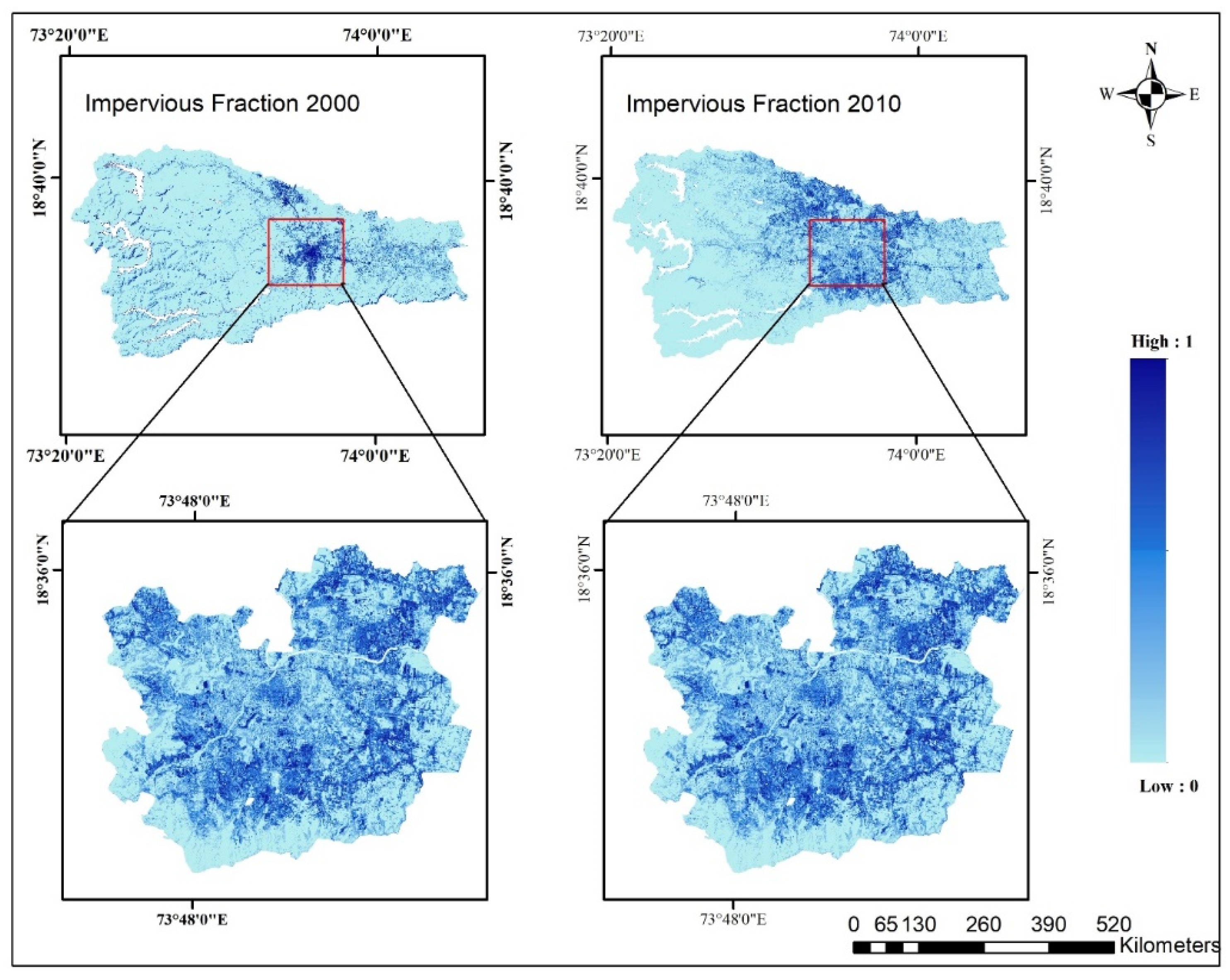
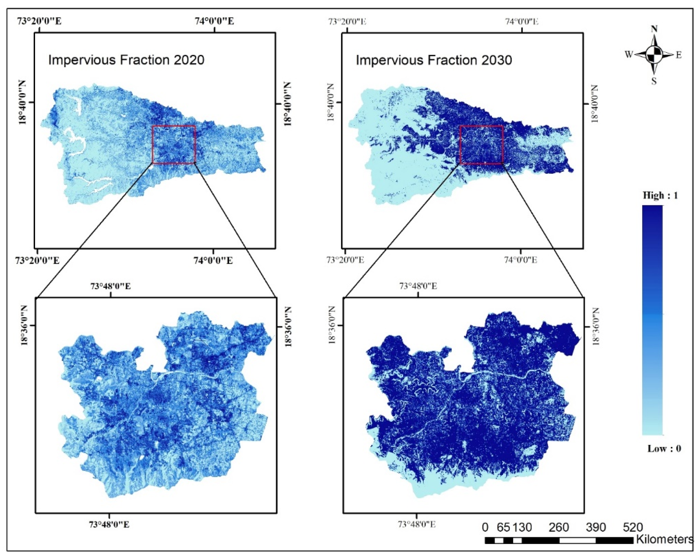
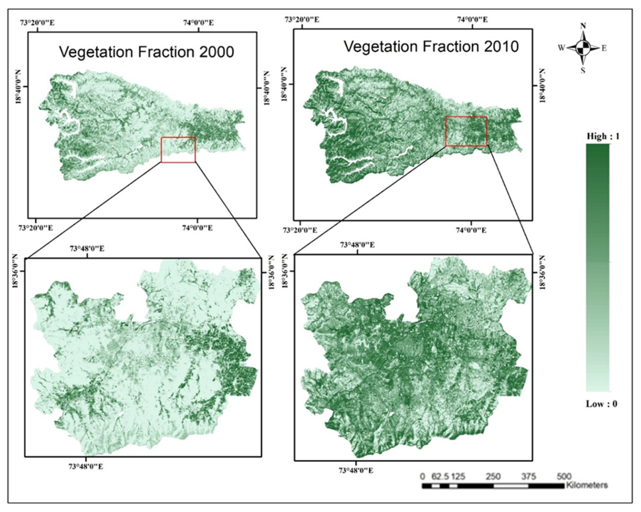
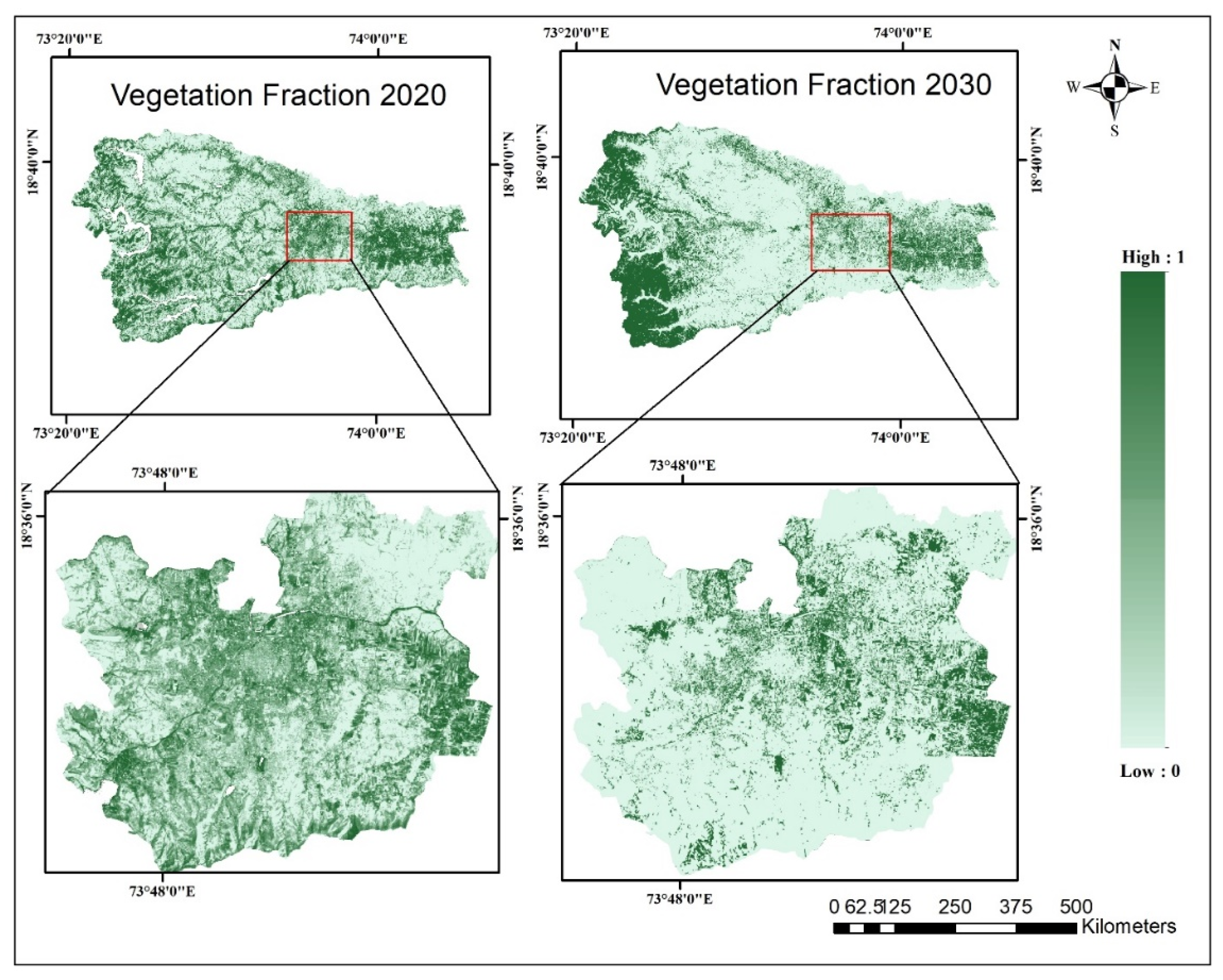
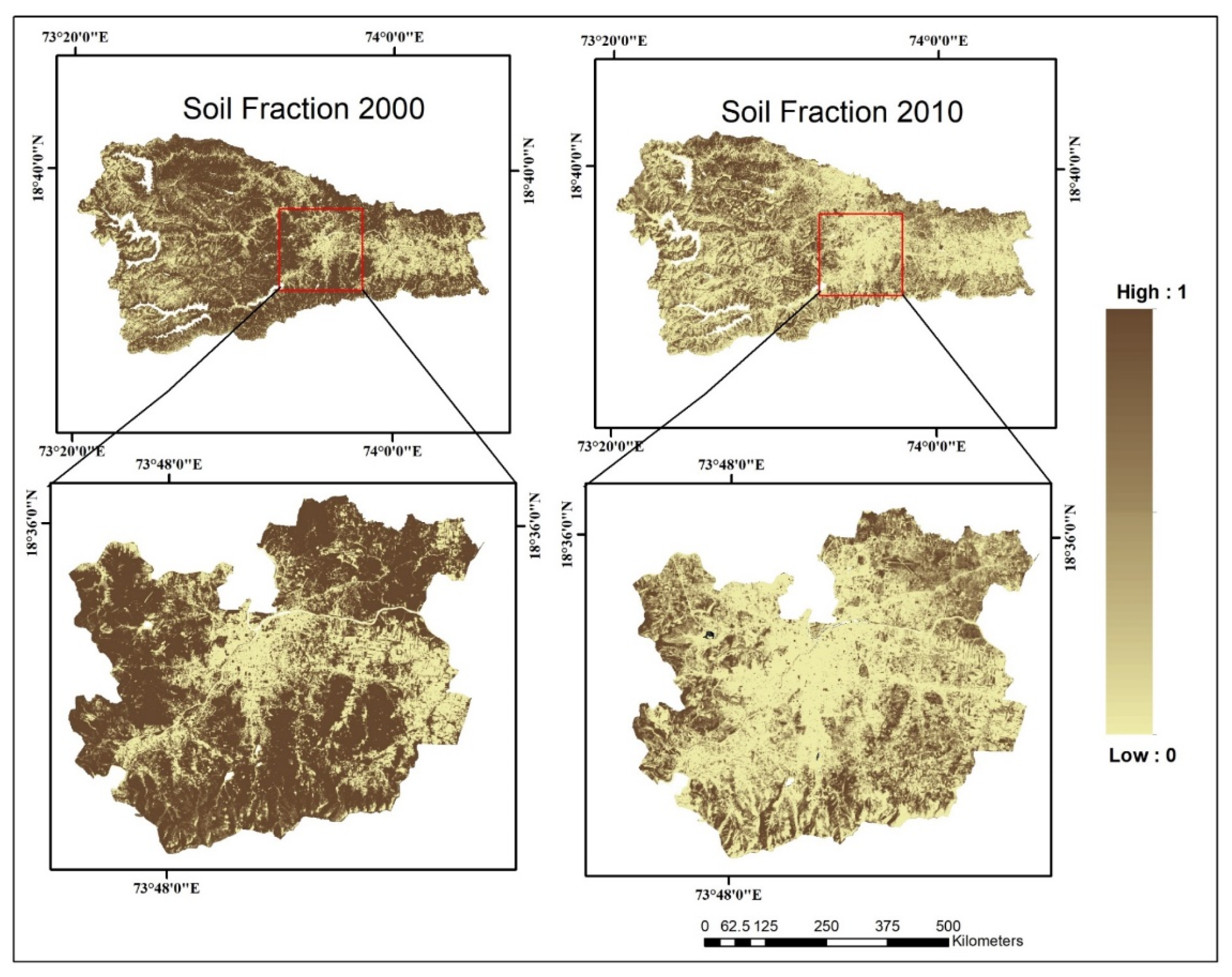
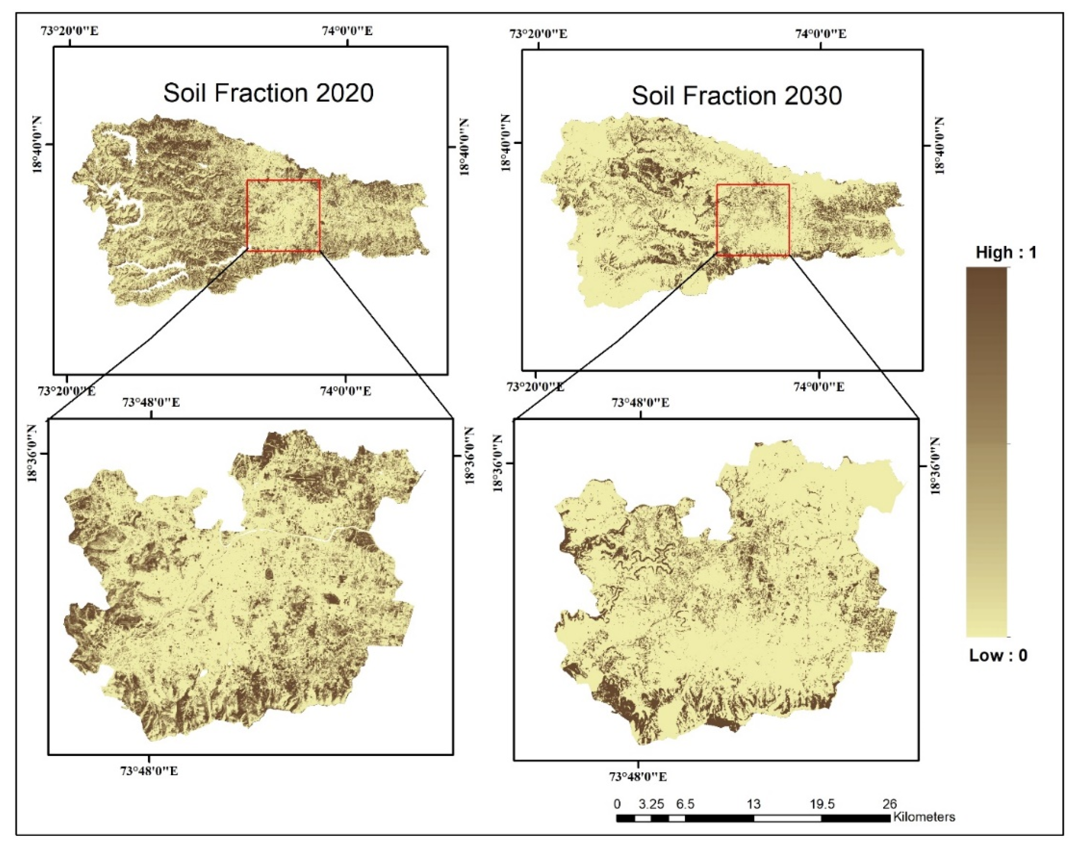
Urbanization trends for the years 2000, 2010, 2020, and 2030 were examined using impervious surface analysis (Figure 6 and Figure 7). The results reveal a pattern of rapid and expansive urban growth, particularly concentrated in the peripheral regions of the Pune district. This expansion is primarily driven by the development of robust infrastructure, the establishment of educational institutions, and the growth of industrial zones. Consequently, the proportion of impervious surfaces has markedly increased, leading to concerns regarding reduced surface permeability. These changes amplify the likelihood of urban flooding and waterlogging, particularly during monsoonal periods, due to disrupted natural drainage and diminished infiltration. Vegetation fraction maps for the years 2000, 2010, 2020, and 2030 (Figure 8 and Figure 9) illustrate a progressive and substantial decline in natural vegetation across the region. This reduction is attributed to accelerating urban and industrial development, which has systematically transformed vegetated landscapes into densely built-up zones. The expansion of impervious surfaces not only inhibits groundwater recharge but also intensifies surface runoff and flood vulnerability. These impacts are especially pronounced in urban and peri-urban areas, where the natural land cover has been mostly altered. The decline in vegetation cover is particularly evident in central business districts and along major transportation corridors, where land transformation has been most pronounced. Similarly, the soil fraction maps (Figure 10 and Figure 11) across the four decades demonstrate significant transformation of soil composition and structure, largely driven by unregulated urban expansion. These maps use a normalized index ranging from zero to one, with higher values representing greater visible soil cover and lower values indicating reduced exposure due to urban encroachment. The predominant soil types in the region, clay and clay loam, have exhibited a marked reduction in bare soil areas, which suggests a progressive sealing of the land surface. This phenomenon has resulted in reduced soil permeability and elevated surface runoff, thereby increasing susceptibility to erosion and stormwater accumulation.

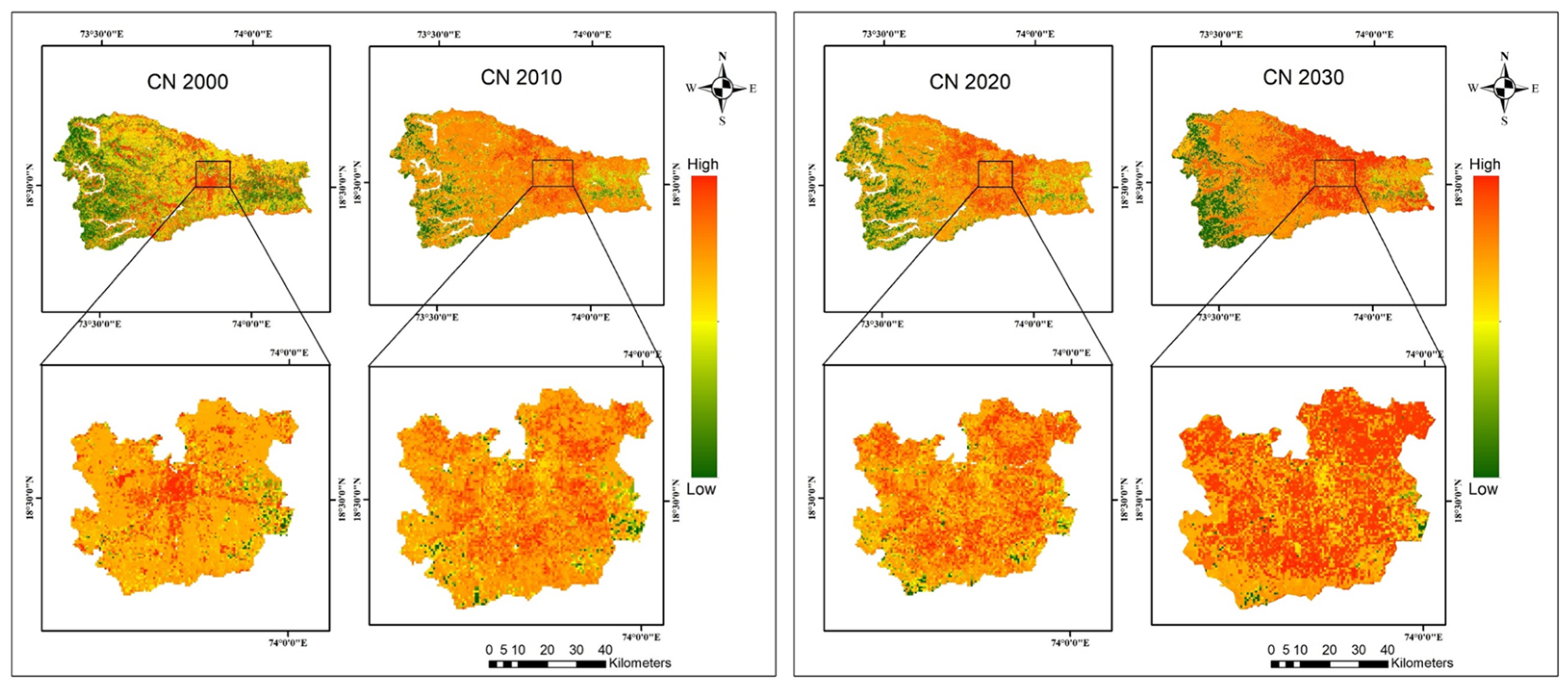
By 2010, a noticeable increase in vegetation cover was observed in peri-urban regions, as reflected in the elevated NDVI values. This trend, however, has reversed in the following decade. NDVI map for 2020 indicates a decline in urban greenery, concurrent with the emergence of new settlements. This pattern highlights the continuing process of urbanization and the associated land use transformation that are exerting pressure on existing vegetation cover. To ensure the reliability of V-I-S fraction maps, an accuracy assessment was conducted using high-resolution imagery from Google Earth. One hundred randomly selected polygons, each representing distinct V-I-S classes, were analyzed for this purpose. The resulting evaluation showed an overall classification accuracy of 88%, with an RMSE of 0.28. These results confirm the satisfactory performance of V-I-S fraction methodology as adopted in the study. CN maps (Figure 12) derived from the integration of V-I-S fraction and NDVI datasets reveal a spatial pattern of hydrological response influenced by land surface characteristics. Areas exhibiting higher CN values are predominantly those with a higher proportion of impervious surfaces and reduced vegetation and soil coverage. Pune city displayed the highest CN values, with a marked upward trend over the study period. This increase is especially evident along major road networks, signifying the intensified impervious surface development. The rising CN values suggest a growing vulnerability to surface runoff, highlighting the hydrological consequences of rapid urban expansion and vegetation loss.

4.3. Analysis of Water Balance Components

The bias-corrected simulations from the General Circulation Models (ACCESS CM2 and MPI ESM 1.2 HR) were assessed for precipitation, maximum temperature (Tmax), and minimum temperature (Tmin). Among the four bias correction approaches used, i.e., Linear Scaling Method (LSM), Power Transformation (PT), Local Intensity Scaling (LOCI), and Distribution Mapping (DM), the LSM and DM showed the most stable and satisfactory performance. For rainfall, LSM with the MPI ESM 1.2 HR model provided the lowest Mean Absolute Error (MAE) of 2.65 mm/month and the lowest Root Mean Square Error (RMSE) of 6.39 mm/month, together with Nash–Sutcliffe Efficiency (NSE) of 0.49 and a coefficient of determination (R²) of 0.71. Conversely, DM performed better than other techniques in temperature correction; with MPI ESM 1.2 HR having NSE values of 0.80 and 0.88 for Tmax and Tmin, respectively, and respective R² values of 0.90 and 0.94. The findings emphasize that though DM performs better in temperature bias correction, LSM is better suited for precipitation in the study area (

Table 1. Performance evaluation of bias correction technique using statistical metrics.

GCM	Performance Statistics	Precipitation (mm)		Tmax (°C)		Tmin (°C)
		LSM	DM	LSM	DM	LSM	DM
ACCESS CM2	MAE	2.80	4.09	1.25	1.24	1.51	1.52
	RMSE	6.58	8.95	1.57	1.55	1.88	1.88
	NSE	0.48	0.05	0.63	0.64	0.58	0.59
	R2	0.63	0.51	0.90	0.91	0.92	0.92
MPI-ESM1.2-HR	MAE	2.65	3.40	1.10	0.92	0.87	0.73
	RMSE	6.39	7.17	1.41	1.16	1.21	1.03
	NSE	0.49	0.38	0.71	0.80	0.83	0.88
	R2	0.71	0.65	0.87	0.90	0.92	0.94

, Supplementary Figures S4–S15).

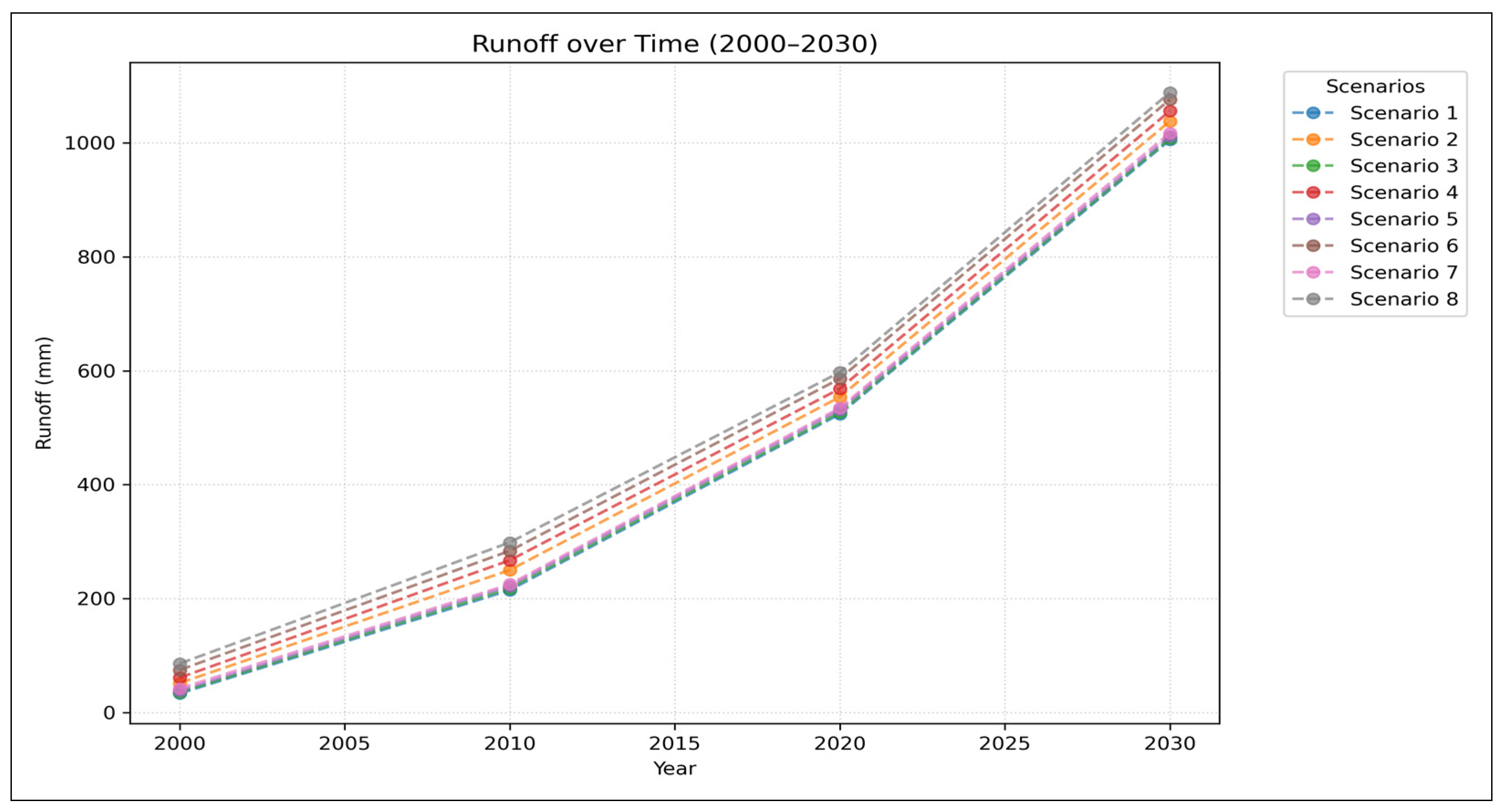
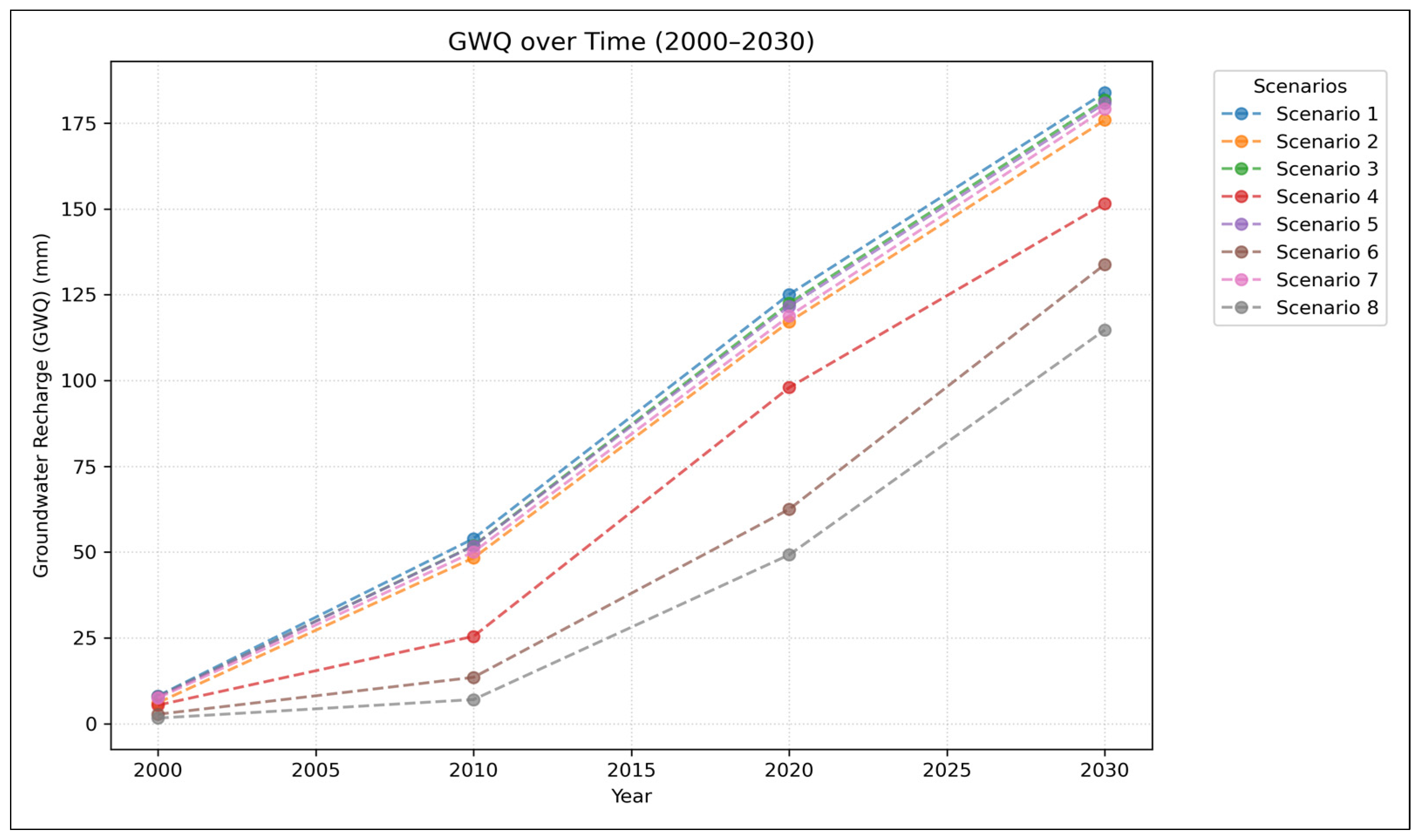
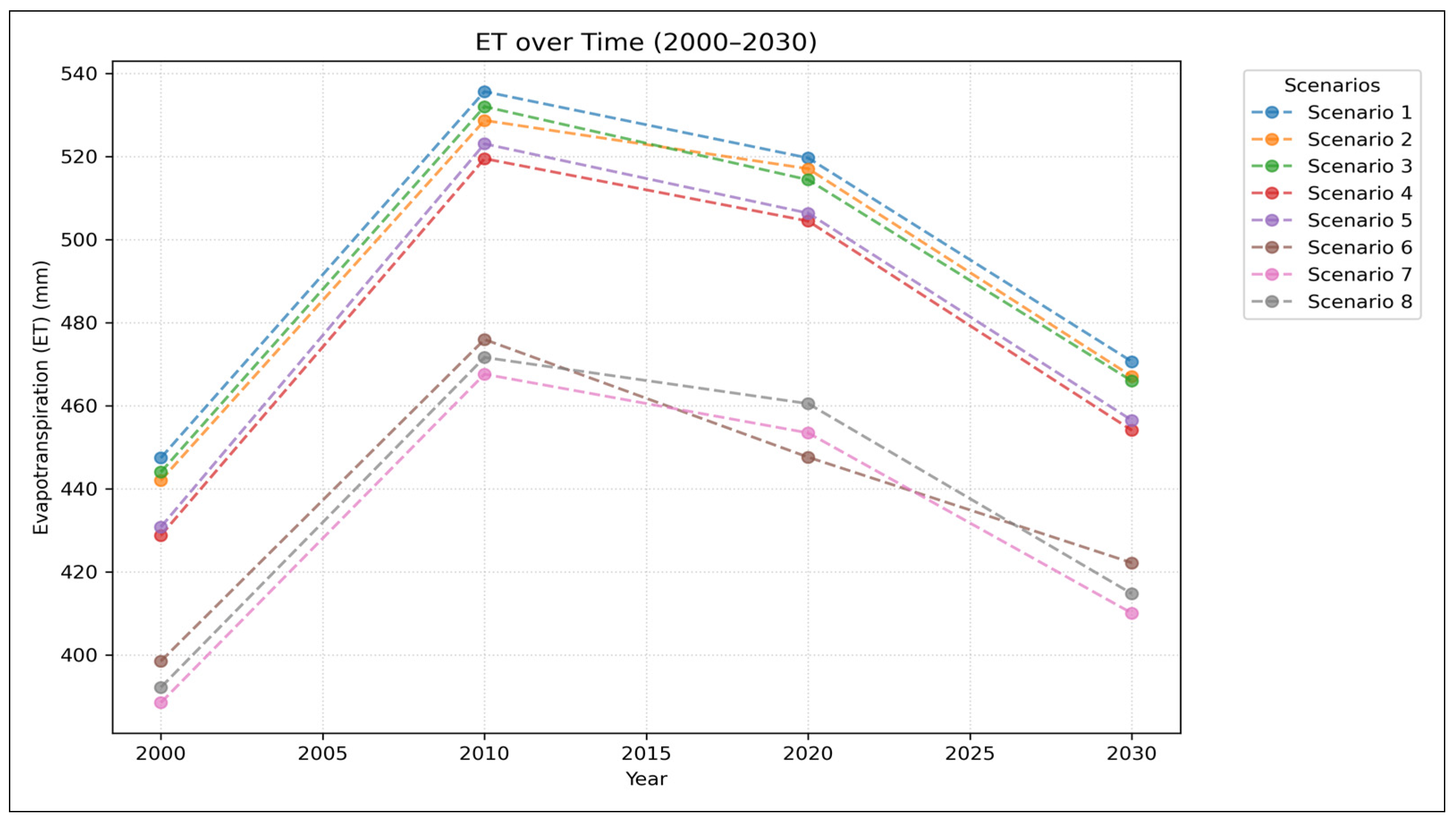
Between 2000 and 2030, a comprehensive assessment was carried out to evaluate the impact of urbanization on major components of water balance. This analysis was performed at a ten-year interval under constant meteorological conditions to isolate the effects of LULC changes. The results indicate that urbanization has significantly altered the hydrological regime, particularly by increasing surface runoff, reducing groundwater recharge, and decreasing evapotranspiration. Surface runoff values demonstrate a marked increase over the study period. When precipitation data from the year 2000 were applied to various LULC scenarios (

Table 2. Description of land use/land cover and composite Curve Number scenarios.

S. No.	Scenario	Description
1	Scenario 1	LULC of the year 2000
2	Scenario 2	Composite CN integrated for the year 2000
3	Scenario 3	LULC of the year 2010
4	Scenario 4	Composite CN integrated for the year 2010
5	Scenario 5	LULC of the year 2020
6	Scenario 6	Composite CN integrated for the year 2020
7	Scenario 7	LULC of the year 2030
8	Scenario 8	Composite CN integrated for the year 2030

), the resulting runoff volumes range from 33.23 mm in Scenario 1 (representing the least urbanized condition) to 85.71 mm in Scenario 8 (representing the most urbanized condition) (Figure 13). This increase reflects the widespread conversion of permeable surfaces to impervious ones, which restricts infiltration and accelerates surface water accumulation. Groundwater recharge exhibited a consistent declining trend (Figure 14). In the year 2000, recharge values varied from 8.1 mm in Scenario 1 to only 1.6 mm in Scenario 8. This decline illustrates how urban expansion reduces the land’s capacity to absorb and store precipitation, thereby compromising long-term groundwater sustainability. Evapotranspiration, an essential component of the water cycle, which is critical for atmospheric moisture exchange, also showed a reduction across the scenarios (Figure 15). In 2000, evapotranspiration rates ranged from 447.4 mm in Scenario 1 to 392.2 mm in Scenario 8. This decline is attributed to the loss of vegetation and exposed soil surfaces. As vegetation is replaced by built-up areas, the land’s ability to return water to the atmosphere through evapotranspiration diminishes.

The relative proportions of the primary water balance components, such as surface runoff, groundwater recharge, and evapotranspiration, were systematically evaluated for the years 2000, 2010, 2020, and projected conditions for 2030 (Supplementary Figure S3). In 2000, the surface runoff comprised approximately 47% of total water budget, groundwater recharge contributed 10%, and evapotranspiration accounted for 43%. By 2010, surface runoff had increased marginally to 49%, while groundwater recharge remained constant at 10%. However, evapotranspiration experienced a sharp decline to 8%, likely reflecting an abrupt reduction in vegetation and permeable surfaces due to urban expansion. In 2020, surface runoff further increased to 53%, groundwater recharge decreased to 6%, and evapotranspiration slightly recovered to 41%, possibly due to localized vegetative efforts or changes in land surface characteristics. Projections for 2030 indicate a continued rise in surface runoff to 54%, a further decline in groundwater recharge to 5%, and stabilization of evapotranspiration at 41%. These temporal trends underscore the growing hydrological imbalance associated with urbanization. The continuous increase in surface runoff is a direct consequence of the proliferation of impervious surfaces, which restricts water infiltration and increases flood risks. Meanwhile, the steady decline in groundwater recharge threatens long-term water security, and the fluctuating evapotranspiration rates reflect changes in vegetative cover and soil moisture availability.

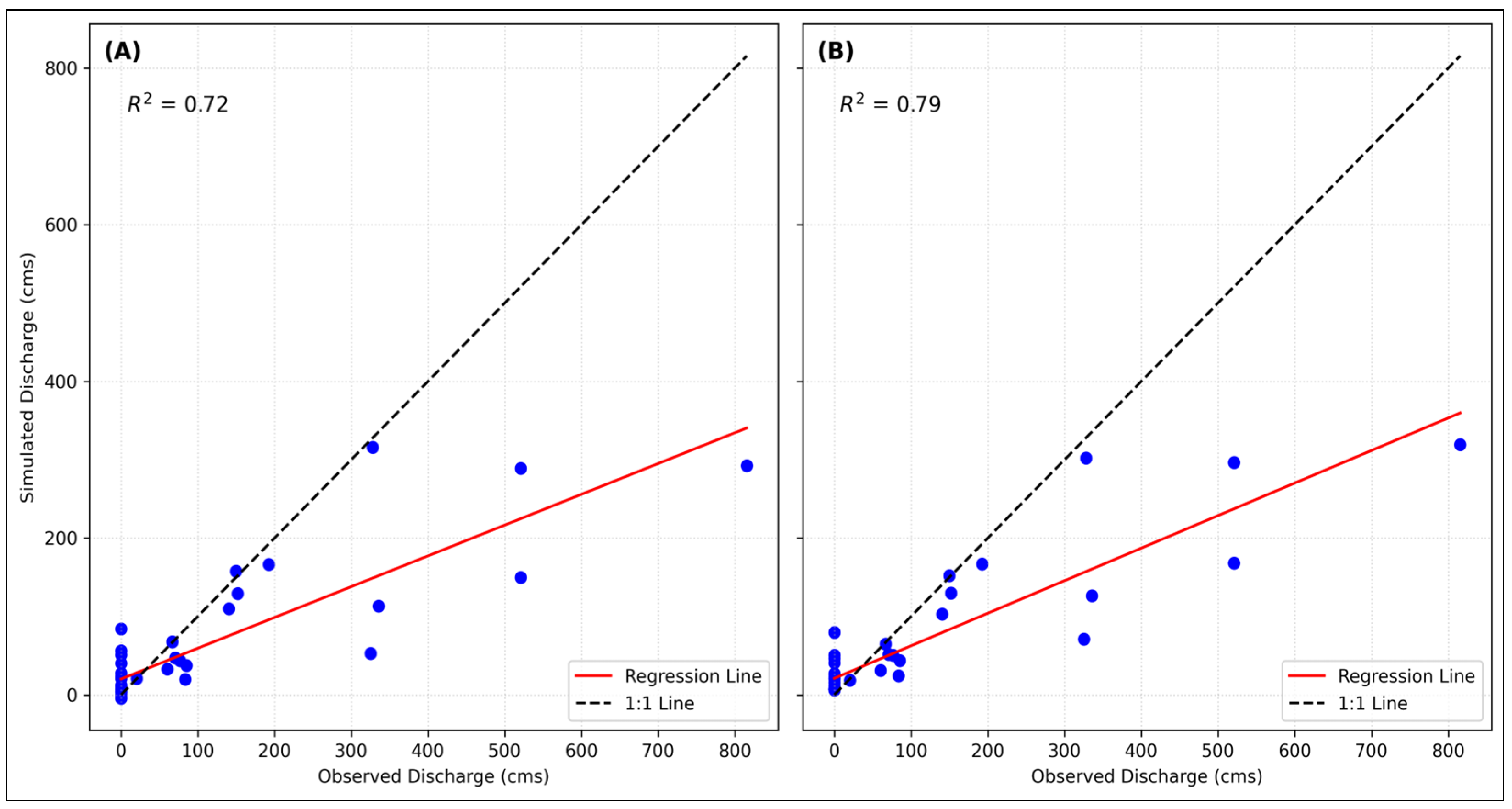
In addition to the climate data correction, model validation was also conducted using observed discharge data from the Mirawadi basin for the period 2018 to 2021. Two distinct scenarios were considered: (i) simulation using the 2020 LULC dataset, and (ii) simulation using the CN values derived from the V-I-S ratio for 2020 (Figure 16). LULC-based simulation achieved an R² of approximately 0.72, while the V-I-S-based CN simulation yielded a higher R² of 0.79. These findings validate the model’s reliability and its capability to accurately represent hydrological dynamics in the Mirawadi basin, particularly when CN values are informed by detailed surface composition metrics such as the V-I-S ratio.

4.4. Limitations of the Study

While the suggested approach has helped to quantify hydrological parameters at a temporal scale and as a function of urbanization and climatic indicators, some constraints need to be considered when deciding on its extension to other spatial settings. The reliability of water balance estimation depends on spatial resolution and thematic precision of input data, especially LULC and soils. Urban morphological variability, such as the variations in configurations of impervious surfaces, building typology, and drainage, can affect the transferability of the composite CN method developed from V-I-S (vegetation–impervious surface-soil) fraction maps. The SWAT model is also sensitive to locally specific hydrology and climate conditions, requiring region-specific calibration and validation to maintain the model’s fidelity. Thus, for more general applicability, such methodological assumptions and dependencies need to be critically assessed to preserve the reliability and integrity of hydrological predictions in varied urban terrain.

5. Conclusions

This study conducts a meticulous examination of urban water balance dynamics in MMRC from 2000 to 2030, with a specific focus on the implications of urbanization trends. Using the SWAT hydrological model, it scrutinizes key components such as runoff, groundwater recharge, and evapotranspiration by integrating data from land cover, DEM, and soil maps. Initial analyses comprehensively assess LULC dynamics, with trend projections extending to 2030. Using the temporal remote sensing datasets, the urban growth is quantified, and its impact is assessed by spatially analyzing changes in runoff, groundwater recharge, and evapotranspiration over multiple decades through data-driven simulations. The projections indicate continued urban growth by 2030. In addition, the study introduces novel methodologies, including V-I-S fraction maps and composite CN maps, to provide a more nuanced representation of impervious surfaces. These approaches incorporate essential urban features such as roads and pavements, thereby enhancing the accuracy of urban water balance estimations. The comparative analyses highlight the effectiveness of composite CN derived from V-I-S fraction maps for accurate water balance assessments, offering a robust alternative to conventional LULC-based methods.

The findings quantitatively demonstrate a notable increase in urban area, rising from 14 percent in 2000 to 25 percent in 2020 and projected to reach 34% by 2030. This expansion is accompanied by an increase in runoff, which has grown from 47 percent in 2000 to 53 percent in 2020, and is anticipated to reach 54 percent by 2030. Conversely, groundwater contribution has declined from 10 percent in 2000 to six percent in 2020, with a further expected decrease to four percent by 2030. These results not only highlight hydrological consequences but also the complexity of modelling such impacts, despite using physically based frameworks like SWAT. Looking ahead, the use of high-resolution datasets is recommended for LULC forecasting and hydrological modelling to achieve finer results. Moreover, deep learning approaches may be explored for the integration of sub-pixel level composite CN values, enabling more precise estimation of water balance components. The outcomes of this study hold significant potential for informing future regional planning and the selection of effective adaptation strategies in response to ongoing urbanization and associated hydrological changes.

The results indicate an increase in surface runoff and a reduction in infiltration and soil moisture across the study period. These changes are closely linked to the expansion of impervious surfaces and alterations in seasonal rainfall distribution. By integrating V-I-S-derived composite CN, the model achieves greater precision in runoff estimation and better captures the hydrological consequences of mixed urban land cover. The study thus presents a scalable methodology for coupling remote sensing data with hydrological models to produce actionable insights for urban water management. This study contributes to the growing field of urban climate and hydrological modelling by offering a robust, data-enriched framework that informs climate-resilient planning and water-sensitive urban design.

References

1. Vanham, D. A holistic water balance of Austria—How does the quantitative proportion of urban water requirements relate to other users? Water Sci. Technol. 2012, 66, 549–555. [Google Scholar] [CrossRef] [Scilit] [PubMed]
2. Linh, N.H.K.; Pham, T.G.; Pham, T.H.; Tran, C.T.M.; Nguyen, T.Q.; Ha, N.T.; Ngoc, N.B. Land-Use and Land-Cover Changes and Urban Expansion in Central Vietnam: A Case Study in Hue City. Urban Sci. 2024, 8, 242. [Google Scholar] [CrossRef] [Scilit]
3. Dan-Jumbo, N.G.; Metzger, M.J.; Clark, A.P. Urban Land-Use Dynamics in the Niger Delta: The Case of Greater Port Harcourt Watershed. Urban Sci. 2018, 2, 108. [Google Scholar] [CrossRef] [Scilit]
4. Gosain, A.; Rao, S.; Basuray, D. Climate Change Impact Assessment on Hydrology of Indian River Basins. Curr. Sci. 2006, 90, 346–353. [Google Scholar]
5. Willems, P.; Arnbjerg-Nielsen, K.; Olsson, J.; Nguyen, V.T.V. Climate change impact assessment on urban rainfall extremes and urban drainage: Methods and shortcomings. Atmos. Res. 2012, 103, 106–118. [Google Scholar] [CrossRef] [Scilit]
6. Arnone, E.; Pumo, D.; Francipane, A.; La Loggia, G.; Noto, L.V. The role of urban growth, climate change, and their interplay in altering runoff extremes. Hydrol. Process. 2018, 32, 1755–1770. [Google Scholar] [CrossRef] [Scilit]
7. Wang, K.; Onodera, S.I.; Saito, M.; Shimizu, Y. Long-term variations in water balance by increase in percent imperviousness of urban regions. J. Hydrol. 2021, 602, 126767. [Google Scholar] [CrossRef] [Scilit]
8. Nasiri, S.; Ansari, H.; Ziaei, A.N. Simulation of water balance equation components using SWAT model in Samalqan Watershed (Iran). Arab. J. Geosci. 2020, 13, 421. [Google Scholar] [CrossRef] [Scilit]
9. Sett, T.; Nikam, B.R.; Sharma, V.; Shrivastava, V. Quantifying the Human Induced Land Use Land Change Impacts on the Water Balance Components of Forested Watershed by Variable Infiltration Capacity Model. ESS Open Arch. 2023. [Google Scholar] [CrossRef] [Scilit] [PubMed]
10. Fan, F.; Fan, W.; Weng, Q. Improving Urban Impervious Surface Mapping by Linear Spectral Mixture Analysis and Using Spectral Indices. Can. J. Remote Sens. 2015, 41, 577–586. [Google Scholar] [CrossRef] [Scilit]
11. Li, C.; Liu, M.; Hu, Y.; Shi, T.; Zong, M.; Walter, M.T. Assessing the impact of urbanization on direct runoff using improved composite CN method in a large urban area. Int. J. Environ. Res. Public Health 2018, 15, 775. [Google Scholar] [CrossRef] [Scilit] [PubMed]
12. Yadav, P.; Deshpande, S. Assessment of anticipated runoff because of impervious surface increase in Pune Urban Catchments, India: A remote sensing approach. In Proceedings of the Eighth International Conference on Digital Image Processing (ICDIP 2016), Chengu, China, 20–22 May 2016; SPIE: Bellingham, WA, USA, 2016; p. 100333T. [Google Scholar] [CrossRef] [Scilit]
13. Wang, Y.; Chen, A.S.; Fu, G.; Djordjević, S.; Zhang, C.; Savić, D.A. An integrated framework for high-resolution urban flood modelling considering multiple information sources and urban features. Environ. Model. Softw. 2018, 107, 85–95. [Google Scholar] [CrossRef] [Scilit]
14. Rautela, K.S.; Kumar, M.; Sofi, M.S.; Kuniyal, J.C.; Bhat, S.U. Modelling of Streamflow and Water Balance in the Kuttiyadi River Basin Using SWAT and Remote Sensing/GIS Tools. Int. J. Environ. Res. 2022, 16, 37. [Google Scholar] [CrossRef] [Scilit]
15. Wagner, P.D.; Kumar, S.; Schneider, K. An assessment of land use change impacts on the water resources of the Mula and Mutha Rivers catchment upstream of Pune, India. Hydrol. Earth Syst. Sci. 2013, 17, 2233–2246. [Google Scholar] [CrossRef] [Scilit]
16. Kamble, V.B.; Vidyasagar, A.A.; Guldeokar, S.M. Spatio-Temporal Change in Agricultural Land Use Pattern in Pune District Maharashtra. Available online: https://www.saspublishers.com/media/articles/SJAHSS_23A391-395.pdf (accessed on 1 May 2026).
17. Kshirsagar, M.; Satpute, R.; Chavda, D.; Khare, K. Exploring an Approach to Estimate Runoff in an Ungauged Mixed Urban Micro Catchment—A Case Study, Pune, India. Cardiometry 2022, 24, 584–592. [Google Scholar] [CrossRef] [Scilit]
18. Pawar, R.S. Urban Growth Analysis of Pune City Using GIS and Remote Sensing. Int. J. Adv. Sci. Res. 2021, 4, 30–34. [Google Scholar]
19. Butsch, C.; Kumar, S.; Wagner, P.D.; Kroll, M.; Kantakumar, L.N.; Bharucha, E.; Schneider, K.; Kraas, F. Growing ‘Smart’? Urbanization processes in the Pune urban agglomeration. Sustainability 2017, 9, 2335. [Google Scholar] [CrossRef] [Scilit]
20. Essenfelder, A.H. SWAT Weather Database A Quick Guide. 2016. Available online: https://www.researchgate.net/publication/294535100_SWAT_Weather_Database?channel=doi&linkId=56c1995008aeedba0565a47f&showFulltext=true (accessed on 1 May 2026).
21. Senent-Aparicio, J.; Jimeno-Sáez, P.; López-Ballesteros, A.; Giménez, J.G.; Pérez-Sánchez, J.; Cecilia, J.M.; Srinivasan, R. Impacts of swat weather generator statistics from high-resolution datasets on monthly streamflow simulation over Peninsular Spain. J. Hydrol. Reg. Stud. 2021, 35, 100826. [Google Scholar] [CrossRef] [Scilit]
22. Amini, S.; Saber, M.; Rabiei-Dastjerdi, H.; Homayouni, S. Urban Land Use and Land Cover Change Analysis Using Random Forest Classification of Landsat Time Series. Remote Sens. 2022, 14, 2654. [Google Scholar] [CrossRef] [Scilit]
23. Svoboda, J.; Štych, P.; Laštovička, J.; Paluba, D.; Kobliuk, N. Random Forest Classification of Land Use, Land-Use Change and Forestry (LULUCF) Using Sentinel-2 Data—A Case Study of Czechia. Remote Sens. 2022, 14, 1189. [Google Scholar] [CrossRef] [Scilit]
24. Tikuye, B.G.; Rusnak, M.; Manjunatha, B.R.; Jose, J. Land Use and Land Cover Change Detection Using the Random Forest Approach: The Case of The Upper Blue Nile River Basin, Ethiopia. Glob. Chall. 2023, 7, 2300155. [Google Scholar] [CrossRef] [Scilit] [PubMed]
25. Gislason, P.O.; Benediktsson, J.A.; Sveinsson, J.R. Random forests for land cover classification. Pattern Recognit. Lett. 2006, 7, 294–300. [Google Scholar] [CrossRef] [Scilit]
26. Nguyen, H.T.T.; Doan, T.M.; Radeloff, V. Applying Random Forest classification to map Land use/Land cover using Landsat 8 OLI. In Proceedings of the International Archives of the Photogrammetry, Remote Sensing and Spatial Information Sciences—ISPRS Archives, International Society for Photogrammetry and Remote Sensing, Istanbul, Turkey, 18–21 March 2018; pp. 363–367. [Google Scholar] [CrossRef] [Scilit]
27. Tokar, O.; Vovk, O.; Kolyasa, L.; Havryliuk, S.; Korol, M. Using the Random Forest Classification for Land Cover Interpretation of Landsat Images in the Prykarpattya Region of Ukraine. In Proceedings of the 2018 IEEE 13th International Scientific and Technical Conference on Computer Sciences and Information Technologies (CSIT), Lviv, Ukraine, 11–14 September 2018. [Google Scholar] [CrossRef] [Scilit]
28. Ahmad, F.; Goparaju, L.; Qayum, A. LULC analysis of urban spaces using Markov chain predictive model at Ranchi in India. Spat. Inf. Res. 2017, 25, 351–359. [Google Scholar] [CrossRef] [Scilit]
29. Gharaibeh, A.; Shaamala, A.; Obeidat, R.; Al-Kofahi, S. Improving land-use change modeling by integrating ANN with Cellular Automata-Markov Chain model. Heliyon 2020, 6, e05092. [Google Scholar] [CrossRef] [Scilit] [PubMed]
30. Singh, S.K.; Mustak, S.; Srivastava, P.K.; Szabó, S.; Islam, T. Predicting Spatial and Decadal LULC Changes Through Cellular Automata Markov Chain Models Using Earth Observation Datasets and Geo-information. Environ. Process. 2015, 2, 61–78. [Google Scholar] [CrossRef] [Scilit]
31. Hamad, R.; Balzter, H.; Kolo, K. Predicting land use/land cover changes using a CA-Markov model under two different scenarios. Sustainability 2018, 10, 3421. [Google Scholar] [CrossRef] [Scilit]
32. Hyandye, C.; Martz, L.W. A Markovian and cellular automata land-use change predictive model of the Usangu Catchment. Int. J. Remote Sens. 2017, 38, 64–81. [Google Scholar] [CrossRef] [Scilit]
33. Ibarra-Bonilla, J.S.; Villarreal-Guerrero, F.; Prieto-Amparán, J.A.; Santellano-Estrada, E.; Pinedo-Alvarez, A. Characterizing the impact of Land-Use/Land-Cover changes on a Temperate Forest using the Markov model. Egypt. J. Remote Sens. Space Sci. 2021, 24, 1013–1022. [Google Scholar] [CrossRef] [Scilit]
34. Szabó, S.; Gácsi, Z.; Balázs, B. Specific features of NDVI, NDWI and MNDWI as reflected in land cover categories. Landsc. Environ. 2016, 10, 194–202. [Google Scholar] [CrossRef] [Scilit]
35. Green, A.A.; Berman, M.; Switzer, P.; Craig, M.D. A Transformation for Ordering Multispectral Data in Terms of Image Quality with Implications for Noise Removal. IEEE Trans. Geosci. Remote Sens. 1988, 26, 65–74. [Google Scholar] [CrossRef] [Scilit]
36. Ridd, M.K. Exploring a V-I-S (Vegetation-impervious surface-soil) model for urban ecosystem analysis through remote sensing: Comparative anatomy for citiest. Int. J. Remote Sens. 1995, 16, 2165–2185. [Google Scholar] [CrossRef] [Scilit]
37. Okujeni, A.; Canters, F.; Cooper, S.D.; Degerickx, J.; Heiden, U.; Hostert, P.; Priem, F.; Roberts, D.A.; Somers, B.; van der Linden, S. Generalizing machine learning regression models using multi-site spectral libraries for mapping vegetation-impervious-soil fractions across multiple cities. Remote Sens. Environ. 2018, 216, 482–496. [Google Scholar] [CrossRef] [Scilit]
38. Guo, H.; Huang, Q.; Li, X.; Sun, Z.; Zhang, Y. Spatiotemporal Analysis of Urban Environment Based on the Vegetation-Impervious Surface-Soil Model. J. Appl. Remote Sens. 2023, 8, 084597. [Google Scholar] [CrossRef] [Scilit]
39. Fan, F.; Deng, Y.; Hu, X.; Weng, Q. Estimating composite curve number using an improved SCS-CN method with remotely sensed variables in guangzhou, China. Remote Sens. 2013, 5, 1425–1438. [Google Scholar] [CrossRef] [Scilit]
40. Iabchoon, S.; Wongsai, S.; Chankon, K. Mapping urban impervious surface using object-based image analysis with WorldView-3 satellite imagery. J. Appl. Remote Sens. 2017, 11, 046015. [Google Scholar] [CrossRef] [Scilit]
41. Lichtblau, E.; Oswald, C.J. Classification of impervious land-use features using object-based image analysis and data fusion. Comput. Environ. Urban Syst. 2019, 75, 103–116. [Google Scholar] [CrossRef] [Scilit]
42. Owojori, A.; Xie, H. Landsat Image-Based LULC Changes of San Antonio, Texas Using Advanced Atmospheric Correction and Object-Oriented Image Analysis Approaches. 2005. Available online: https://www.isprs.org/proceedings/xxxvi/8-w27/owojori.pdf (accessed on 1 May 2026).
43. Akcay, O.; Avsar, E.O.; Inalpulat, M.; Genc, L.; Cam, A. Assessment of segmentation parameters for object-based land cover classification using color-infrared imagery. ISPRS Int. J. Geo-Inf. 2018, 7, 424. [Google Scholar] [CrossRef] [Scilit]
44. Bovolo, F.; Bruzzone, L.; Carlin, L. A novel technique for subpixel image classification based on support vector machine. IEEE Trans. Image Process. 2010, 19, 2983–2999. [Google Scholar] [CrossRef] [Scilit] [PubMed]
45. Tassi, A.; Gigante, D.; Modica, G.; Di Martino, L.; Vizzari, M. Pixel-vs. Object-based landsat 8 data classification in google earth engine using random forest: The case study of maiella national park. Remote Sens. 2021, 13, 2299. [Google Scholar] [CrossRef] [Scilit]
46. Sisay, E.; Halefom, A.; Khare, D.; Singh, L.; Worku, T. Hydrological modelling of ungauged urban watershed using SWAT model. Model. Earth Syst. Environ. 2017, 3, 693–702. [Google Scholar] [CrossRef] [Scilit]
47. Jaiswal, R.K.; Yadav, R.N.; Lohani, A.K.; Tiwari, H.L.; Yadav, S. Water balance modeling of Tandula (India) reservoir catchment using SWAT. Arab. J. Geosci. 2020, 13, 148. [Google Scholar] [CrossRef] [Scilit]
48. Guug, S.S.; Abdul-Ganiyu, S.; Kasei, R.A. Application of SWAT hydrological model for assessing water availability at the Sherigu catchment of Ghana and Southern Burkina Faso. HydroResearch 2020, 3, 124–133. [Google Scholar] [CrossRef] [Scilit]
49. Her, Y.; Frankenberger, J.; Chaubey, I.; Srinivasan, R. Threshold effects in HRU definition of the soil and water assessment tool. Trans. ASABE 2015, 58, 367–378. [Google Scholar] [CrossRef] [Scilit]
50. Neitsch, S.L.; Arnold, J.G.; Kiniry, J.R.; Williams, J.R.; King, K.W. Soil and Water Assessment Tool Theoretical Documentation. 2005. Available online: https://swat.tamu.edu/media/1292/swat2005theory.pdf (accessed on 1 May 2026).
51. Ameja, L.G. Climate Change Induced Temperature Prediction and Bias Correction in Finchaa Watershed. Am.-Eurasian J. Agric. Environ. Sci. 2018, 18, 324–337. Available online: https://www.researchgate.net/publication/362469576_Climate_Change_Induced_Temperature_Prediction_and_Bias_Correction_in_Finchaa_Watershed (accessed on 1 May 2026).
52. Yeboah, K.A.; Akpoti, K.; Kabo-bah, A.T.; Ofosu, E.A.; Siabi, E.K.; Mortey, E.M.; Okyereh, S.A. Assessing climate change projections in the Volta Basin using the CORDEX-Africa climate simulations and statistical bias-correction. Environ. Chall. 2022, 6, 100439. [Google Scholar] [CrossRef] [Scilit]
53. Das, P.; Zhang, Z.; Ren, H. Evaluation of four bias correction methods and random forest model for climate change projection in the Mara River Basin, East Africa. J. Water Clim. Change 2022, 13, 1900–1919. [Google Scholar] [CrossRef] [Scilit]
54. Luo, M.; Liu, T.; Meng, F.; Duan, Y.; Frankl, A.; Bao, A.; De Maeyer, P. Comparing bias correction methods used in downscaling precipitation and temperature from regional climate models: A case study from the Kaidu River Basin in Western China. Water 2018, 10, 1046. [Google Scholar] [CrossRef] [Scilit]
55. Marhaento, H.; Booij, M.J.; Rientjes, T.H.M.; Hoekstra, A.Y. Attribution of changes in the water balance of a tropical catchment to land use change using the SWAT model. Hydrol. Process. 2017, 31, 2029–2040. [Google Scholar] [CrossRef] [Scilit]
56. Pandi, D.; Kothandaraman, S.; Kuppusamy, M. Simulation of Water Balance Components Using SWAT Model at Sub Catchment Level. Sustainability 2023, 15, 1438. [Google Scholar] [CrossRef] [Scilit]
57. Eini, M.R.; Javadi, S.; Delavar, M.; Gassman, P.W.; Jarihani, B. Development of alternative SWAT-based models for simulating water budget components and streamflow for a karstic-influenced watershed. Catena 2020, 195, 104801. [Google Scholar] [CrossRef] [Scilit]
58. Bo, H.; Dong, X.; Li, Z.; Reta, G.; Li, L.; Wei, C. Analysis of water balance components and parameter uncertainties based on swat model with cmads data and sufi-2 algorithm in huangbaihe river Catchment, China. Nat. Environ. Pollut. Technol. 2020, 19, 637–650. [Google Scholar] [CrossRef] [Scilit]
59. Kumar, N.; Singh, S.K.; Srivastava, P.K.; Narsimlu, B. SWAT Model calibration and uncertainty analysis for streamflow prediction of the Tons River Basin, India, using Sequential Uncertainty Fitting (SUFI-2) algorithm. Model. Earth Syst. Environ. 2017, 3, 30. [Google Scholar] [CrossRef] [Scilit]
60. Siddiqui, A.; Siddiqui, A.; Maithani, S.; Jha, A.K.; Kumar, P.; Srivastav, S.K. Urban growth dynamics of an Indian metropolitan using CA Markov and Logistic Regression. Egypt. J. Remote Sens. Space Sci. 2018, 21, 229–236. [Google Scholar] [CrossRef] [Scilit]
61. Maithani, S. Cellular Automata Based Model of Urban Spatial Growth. J. Indian Soc. Remote Sens. 2010, 38, 604–610. [Google Scholar] [CrossRef] [Scilit]
Figure 1. Geographic extent of the Mula–Mutha river catchment and its urban influence zone.
Urbansci 10 00389 g001
Figure 2. Overall methodological framework.
Urbansci 10 00389 g002
Figure 3. Temporal comparison of land use/land cover in 2000 and 2010.
Urbansci 10 00389 g003
Figure 4. Observed and predicted land use/land cover maps for 2020.
Urbansci 10 00389 g004
Figure 5. Predicted land use/land cover map for the year 2030.
Urbansci 10 00389 g005
Figure 6. Spatial distribution of impervious surface fraction for the years 2000 and 2010.
Urbansci 10 00389 g006
Figure 7. Spatial distribution of impervious surface fraction for the years 2020 and 2030.
Urbansci 10 00389 g007
Figure 8. Spatial distribution of vegetation fraction for 2000 and 2010.
Urbansci 10 00389 g008
Figure 9. Spatial distribution of vegetation fraction for 2020 and 2030.
Urbansci 10 00389 g009
Figure 10. Spatial distribution of soil fraction for 2000 and 2010.
Urbansci 10 00389 g010
Figure 11. Spatial distribution of soil fraction for 2020 and 2030.
Urbansci 10 00389 g011
Figure 12. Spatial distribution of hydrological curve numbers (CN) for 2000, 2010, 2020, and 2030.
Urbansci 10 00389 g012
Figure 13. Simulated runoff trends from 2000 to 2030 under eight historical and projected LULC and composite Curve Number (CN) scenarios. Each dotted line represents one LULC–CN scenario. Scenario descriptions and methodology are provided in Table 2.
Urbansci 10 00389 g013
Figure 14. Simulated ground water recharge (GWQ) trends from 2000 to 2030 under eight historical and projected LULC and composite Curve Number (CN) scenarios. Each dotted line represents one LULC–CN scenario. Scenario descriptions and methodology are provided in Table 2.
Urbansci 10 00389 g014
Figure 15. Simulated evapotranspiration (ET) trends from 2000 to 2030 under eight historical and projected LULC and composite Curve Number (CN) scenarios. Each dotted line represents one LULC–CN scenario. Scenario descriptions and methodology are provided in Table 2.
Urbansci 10 00389 g015
Figure 16. Correlation of observed and simulated discharge using (A) LULC-based and (B) composite CN approaches.
Urbansci 10 00389 g016