
Environmental-Health Vulnerability and Respiratory Mortality in Europe: Evidence from Panel Econometrics, Clustering, and Machine Learning

 , and
, and 
Abstract
1. Introduction
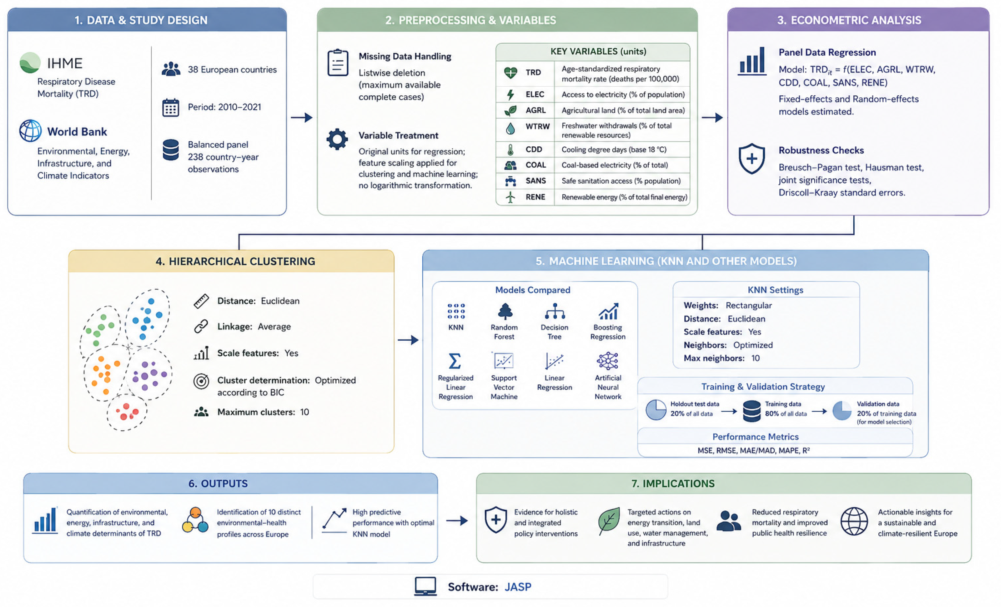
2. Integrated Analytical Framework and Variable Definitions
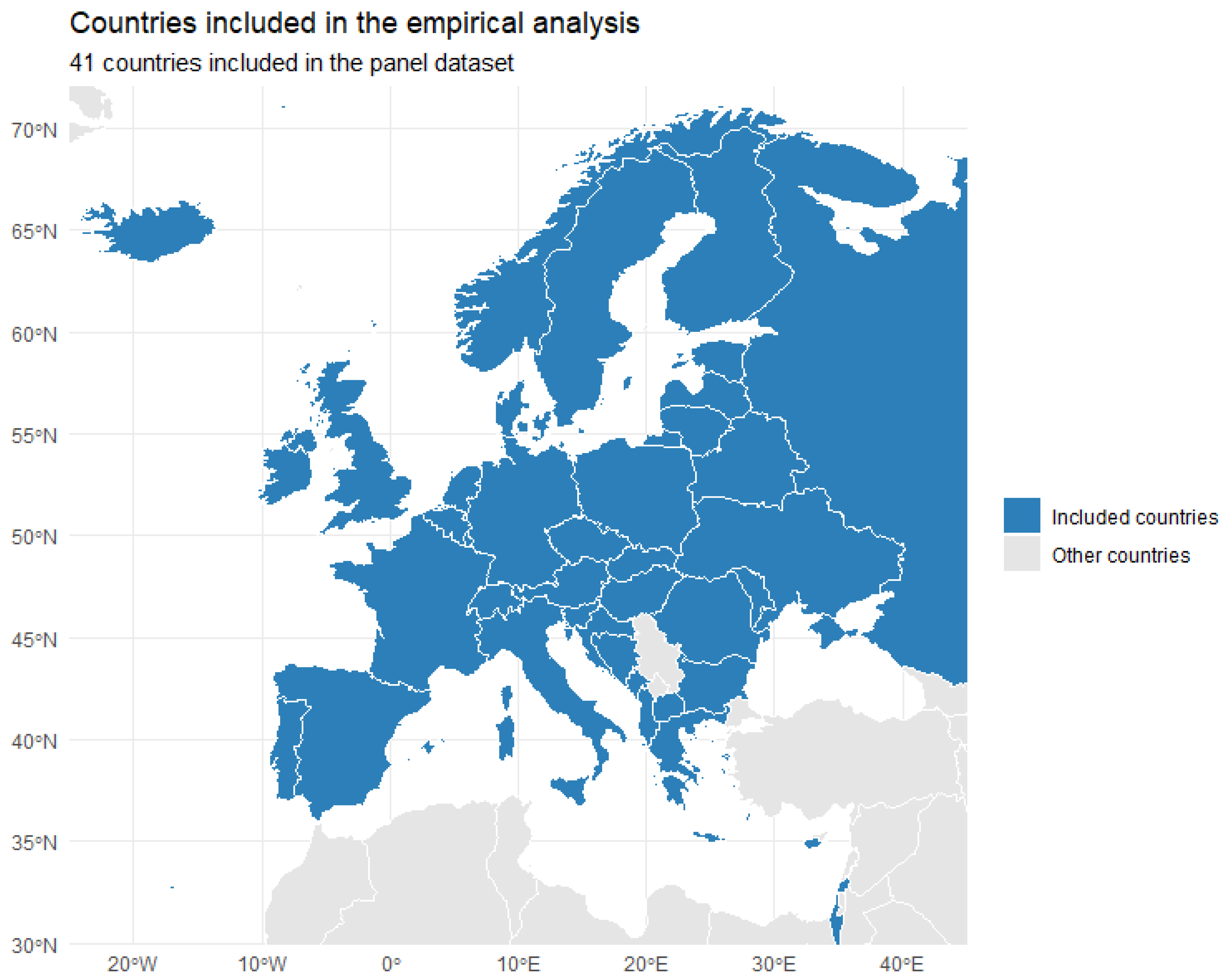
3. Data Harmonization and Multi-Method Analytical Design
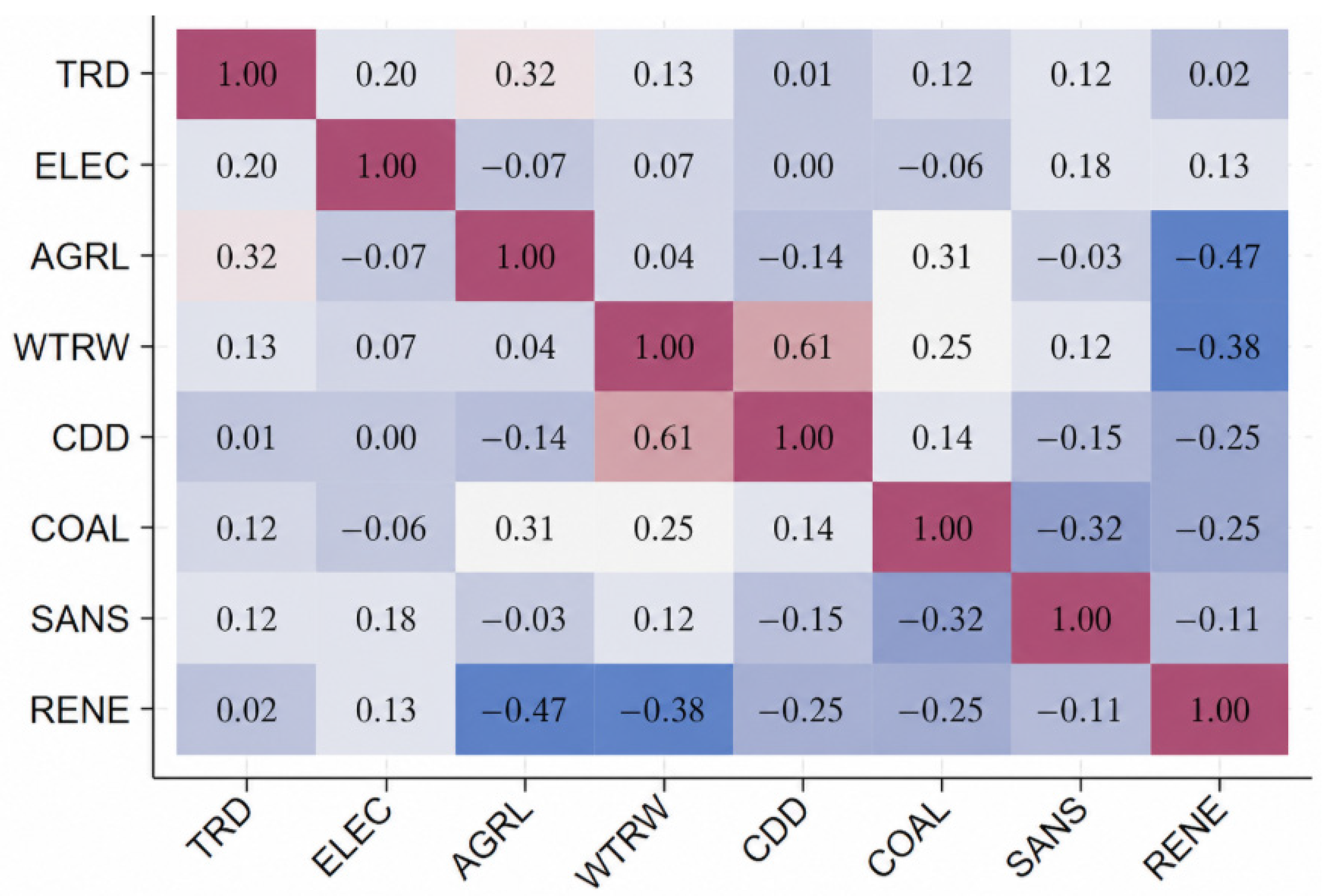
4. Environmental, Infrastructural, and Climatic Associations with Respiratory Mortality
4.1. Robustness Analysis Using Driscoll–Kraay Standard Errors: Addressing Cross-Sectional Dependence and Temporal Correlation
4.2. Sensitivity Analyses and Robustness Checks for Alternative Specifications
4.3. Regional Heterogeneity Between Western and Eastern Europe
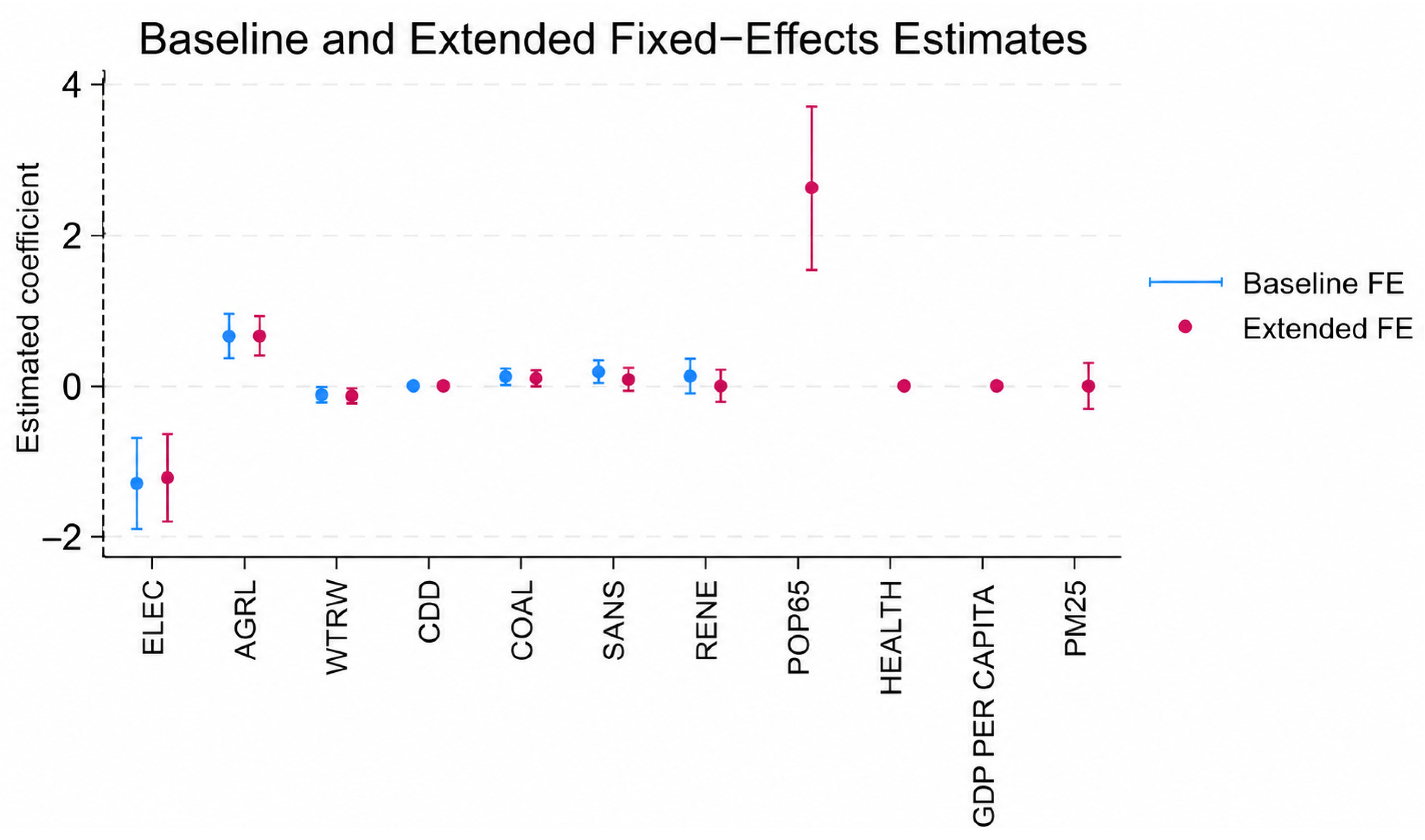
4.4. Extended Fixed-Effects Specification Addressing Potential Omitted-Variable Bias
4.5. Interpreting Structural Environmental and Infrastructure Indicators
4.6. Proxy Effects, Structural Confounding, and Endogeneity
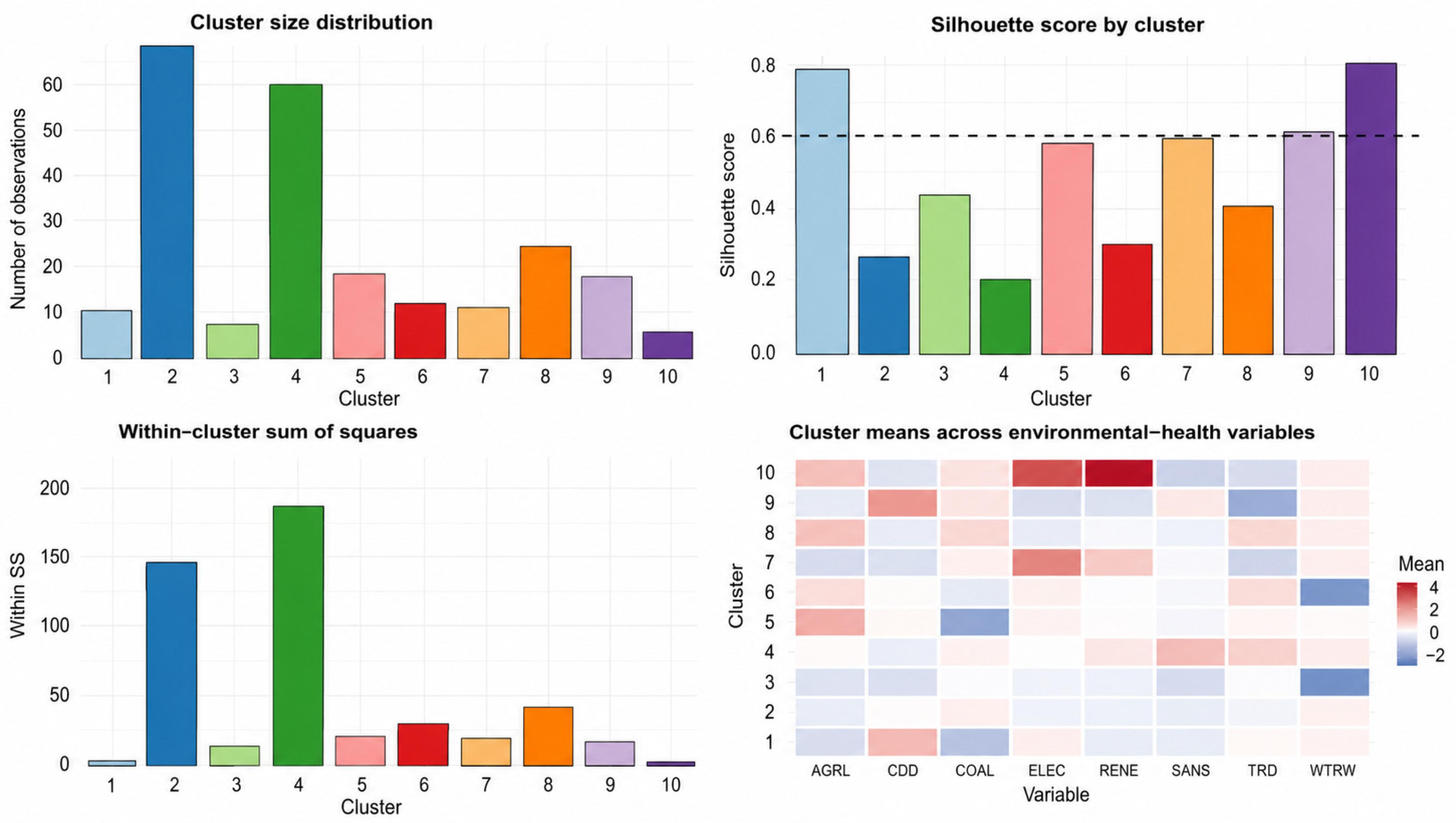
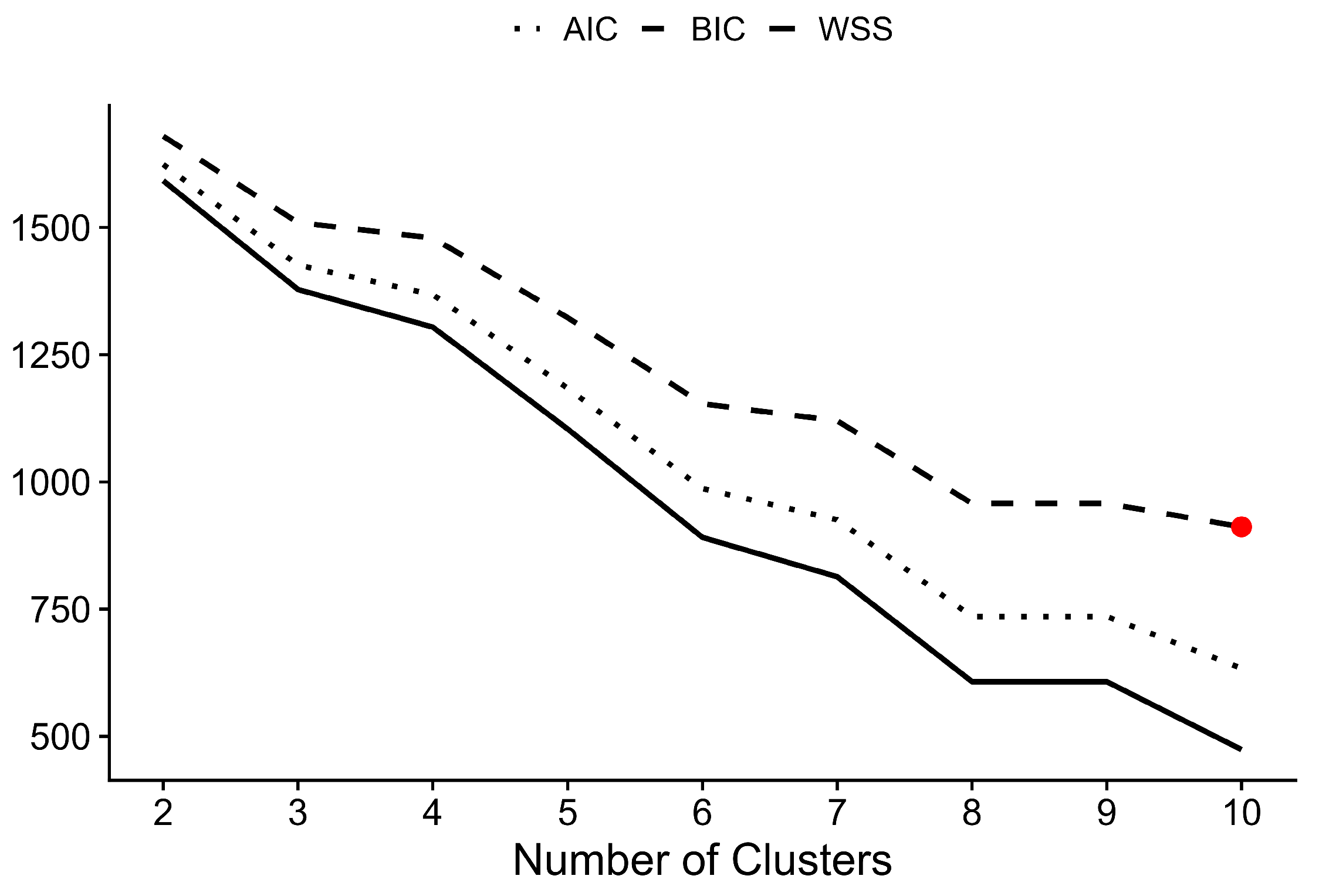
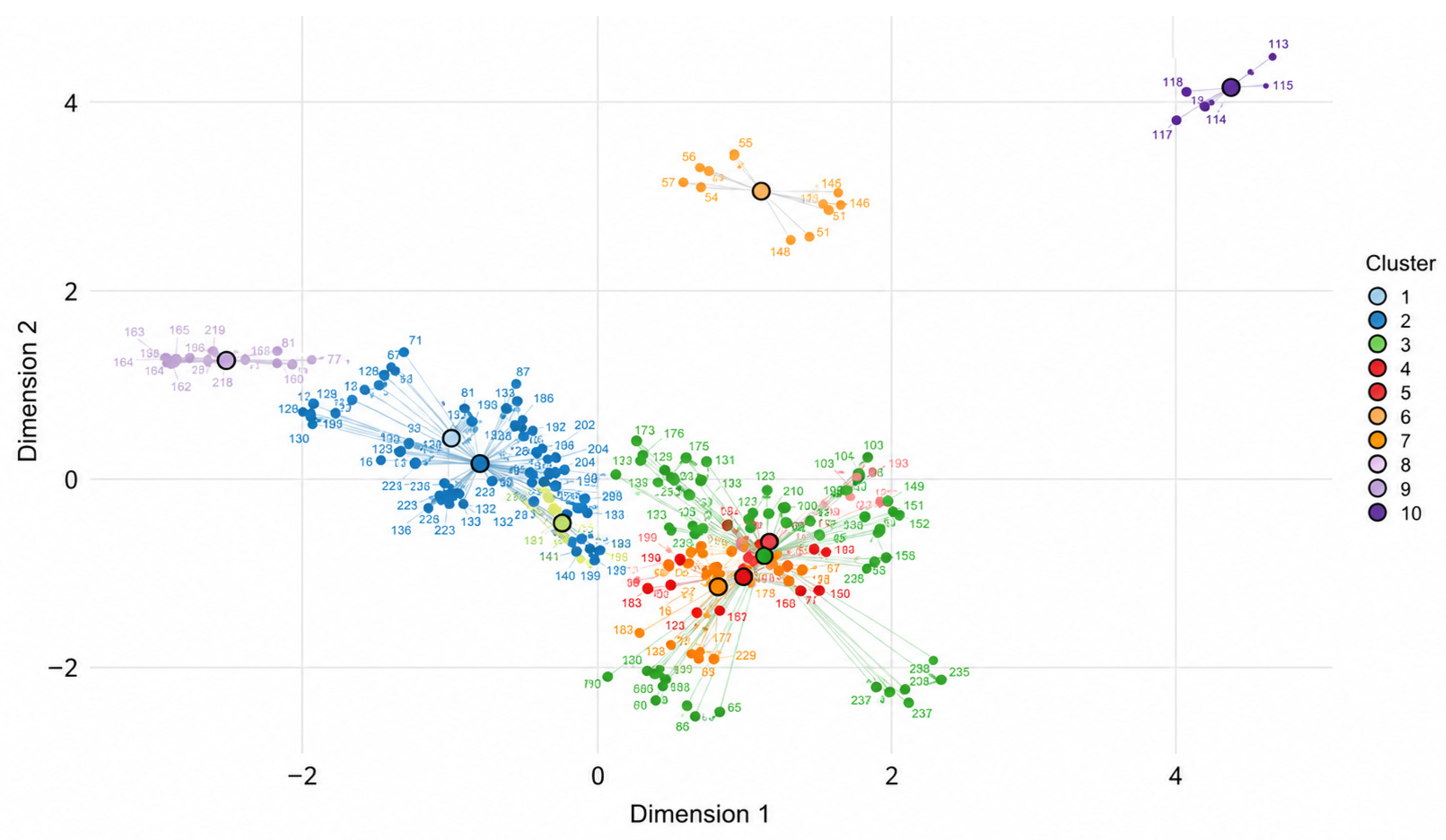
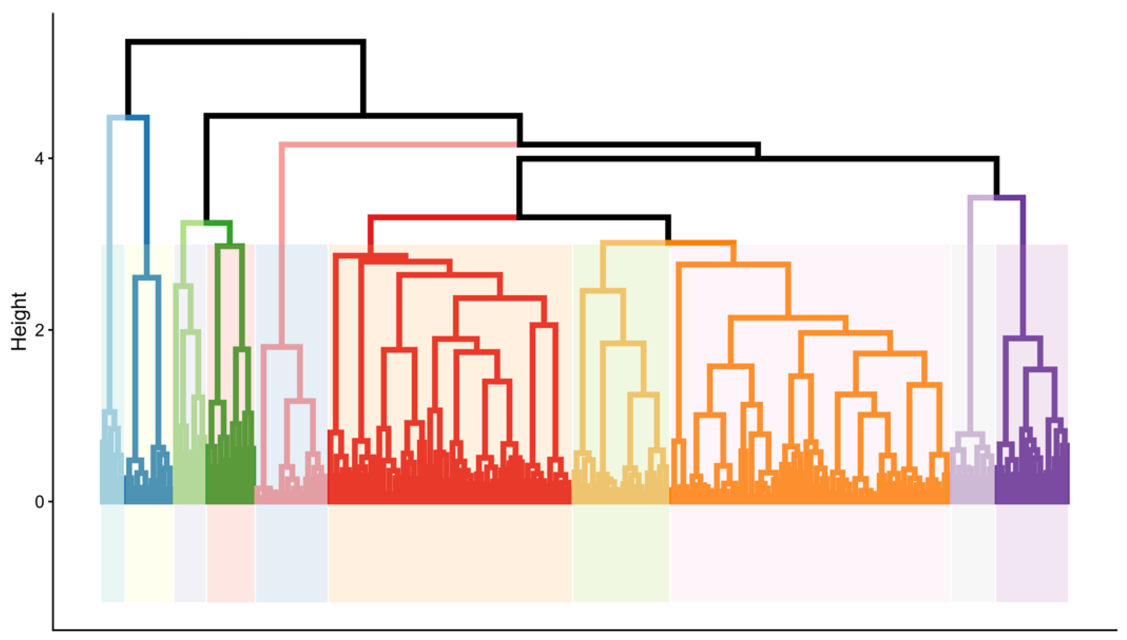
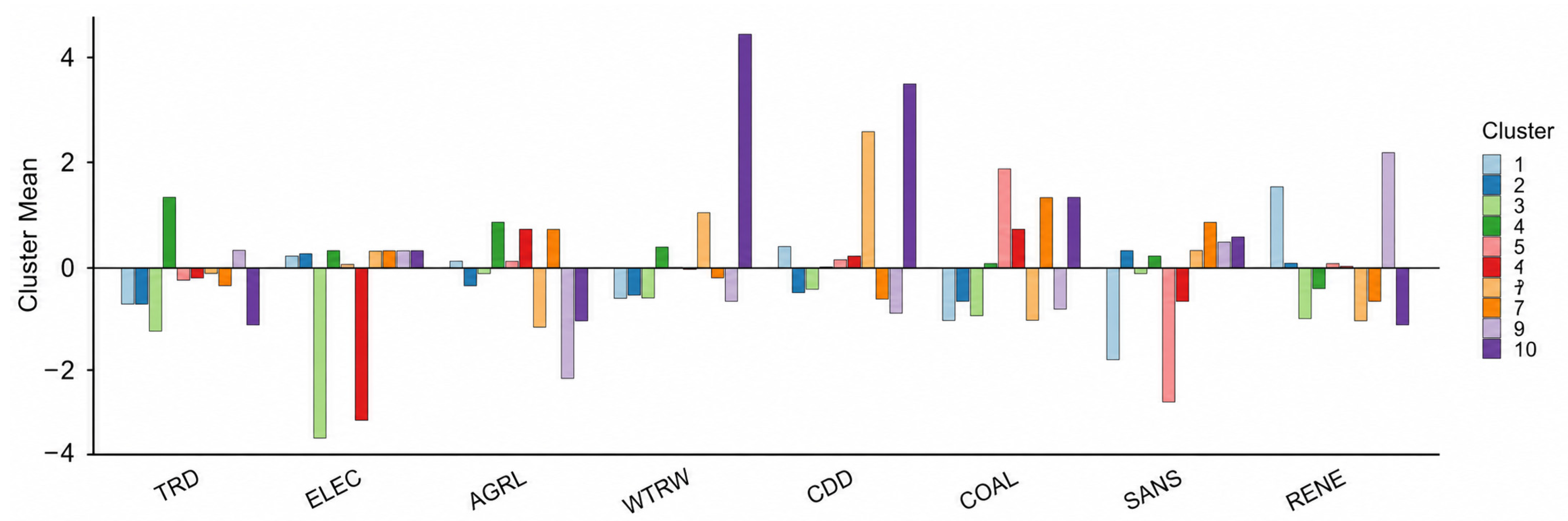
5. Mapping Environmental-Health Vulnerability Through Hierarchical Clustering
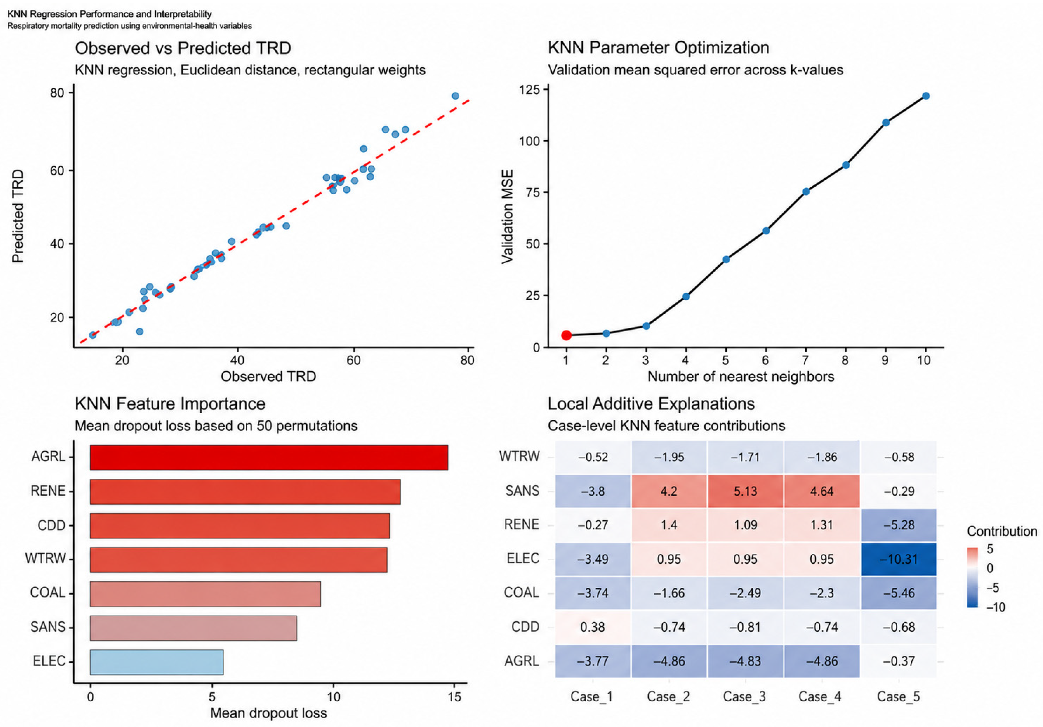
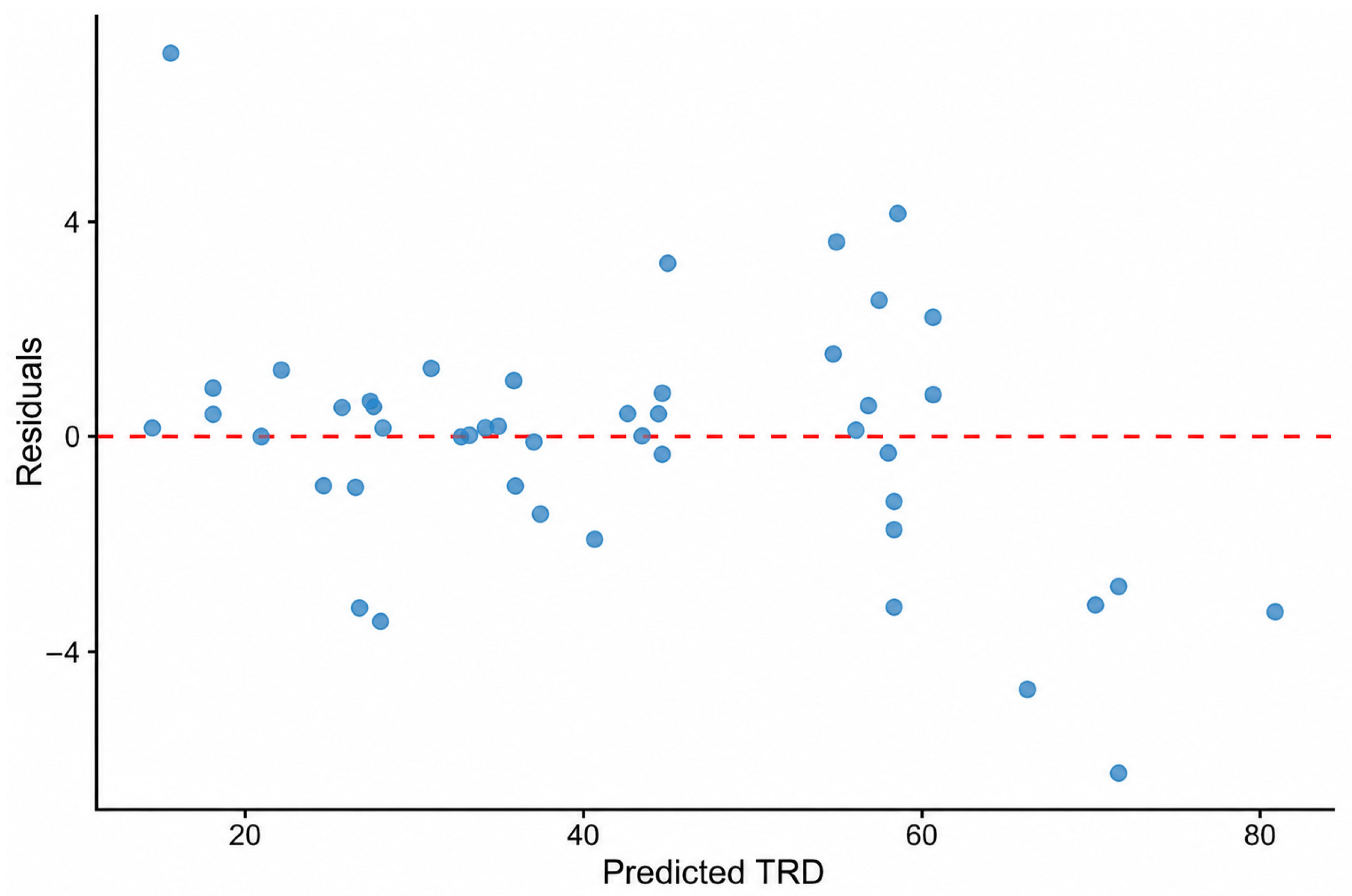
6. Non-Linear Environmental-Health Patterns and Predictive Modelling
6.1. Explaining Environmental-Health Predictions Through Additive Contributions
6.2. Hyperparameter Optimization and Model Configuration
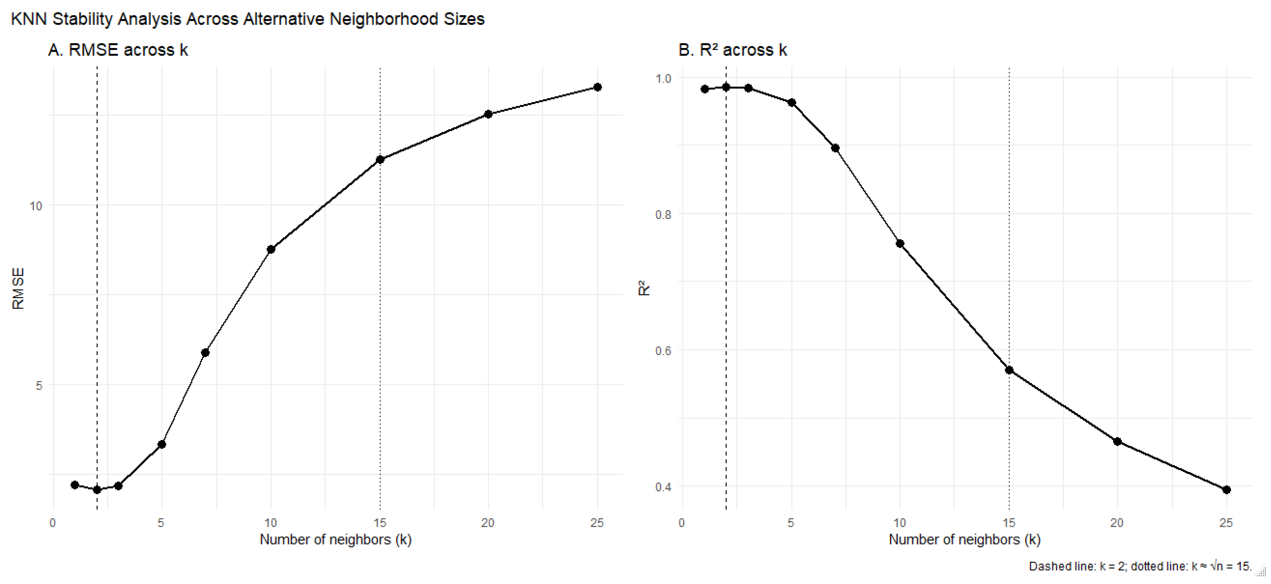
6.3. KNN Stability Across Alternative Neighborhood Specifications
6.4. Limitations and Interpretation of the Machine-Learning Framework
7. Integration of Econometric, Clustering, and Machine-Learning Evidence
8. Limitations in Data, Inference, and Predictive Modelling
9. Urban Vulnerability, Infrastructure Transitions, and Policy Implications
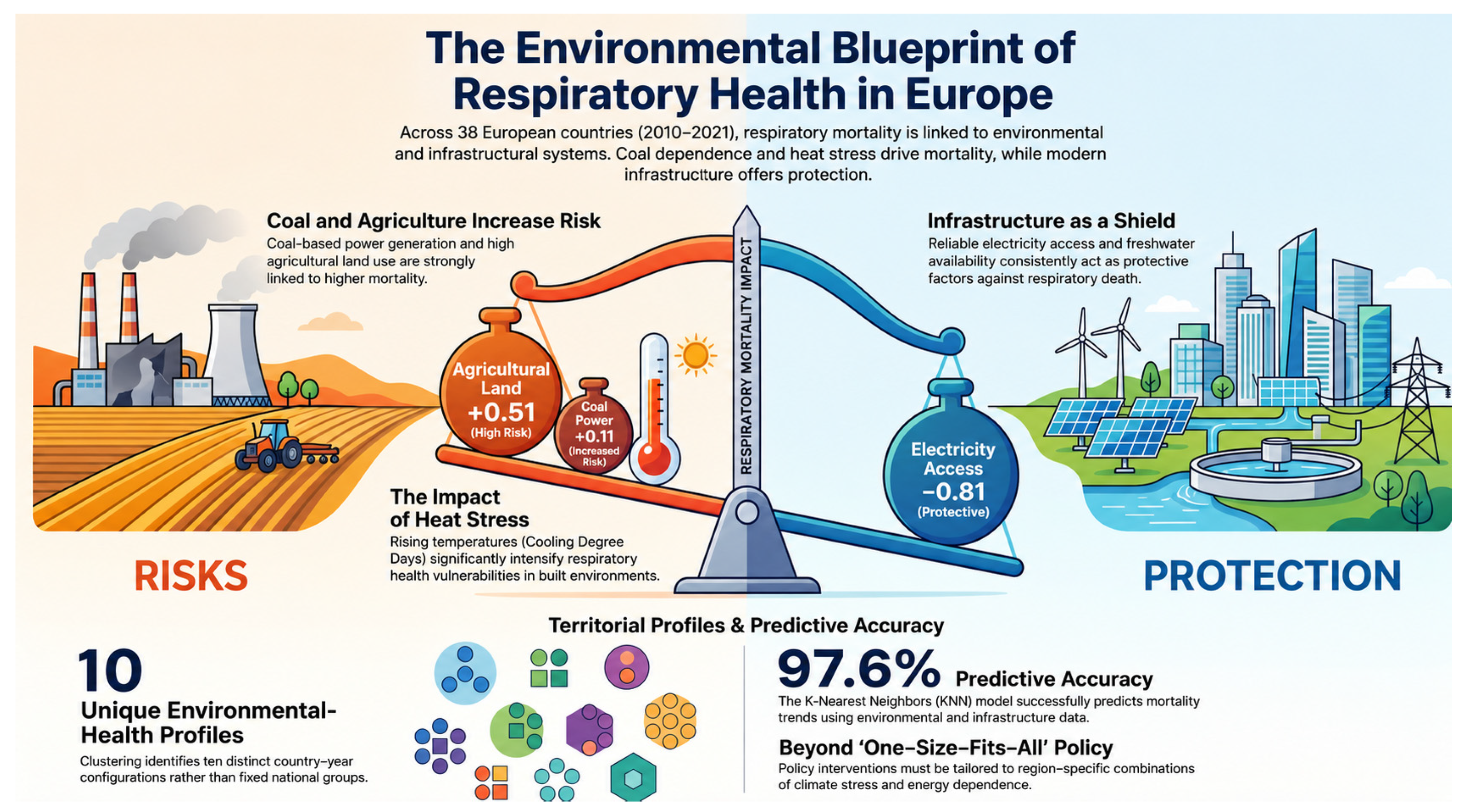
10. Conclusions
Author Contributions
Funding
Institutional Review Board Statement
Informed Consent Statement
Data Availability Statement
Conflicts of Interest
Abbreviations
| Acronym | Definition |
| TRD | Mortality Rate by Respiratory Disease |
| ELEC | Access to Electricity |
| AGRL | Agricultural Land |
| WTRW | Freshwater Withdrawals |
| CDDs | Cooling Degree Days |
| COAL | Coal Electricity |
| SANS | Safe Sanitation |
| RENE | Renewable Energy |
| KNN | K-Nearest Neighbors |
| MSE | Mean Squared Error |
| RMSE | Root Mean Squared Error |
| MAE | Mean Absolute Error |
| MAPE | Mean Absolute Percentage Error |
| SVM | Support Vector Machine |
| ANN | Artificial Neural Network |
References
- Kriit, H.K.; Chen-Xu, J.; Semenza, J.C.; Heiliger, H.; Markandya, A.; Dasandi, N.; Jankin, S.; van Daalen, K.R.; Achebak, H.; Alari, A.; et al. The 2026 Europe report of the Lancet Countdown on health and climate change: Narrowing window for decisive health action. Lancet Public Health 2026, 11, e386–e407. [Google Scholar] [CrossRef] [PubMed]
- Vicedo-Cabrera, A.M.; Melén, E.; Forastiere, F.; Gehring, U.; Katsouyanni, K.; Yorgancioglu, A.; Ulrik, C.S.; Hansen, K.; Powell, P.; Ward, B.; et al. Climate change and respiratory health: A European Respiratory Society position statement. Eur. Respir. J. 2023, 62, 2201960. [Google Scholar] [CrossRef] [PubMed]
- Tran, H.M.; Tsai, F.-J.; Lee, Y.-L.; Chang, J.-H.; Chang, L.-T.; Chang, T.-Y.; Chung, K.F.; Kuo, H.-P.; Lee, K.-Y.; Chuang, K.-J.; et al. The impact of air pollution on respiratory diseases in an era of climate change: A review of the current evidence. Sci. Total Environ. 2023, 898, 166340. [Google Scholar] [CrossRef] [PubMed]
- Im, U.; Ye, Z.; Schuhen, N.; Chowdhury, S.; Christensen, J.H.; Geels, C.; Hänninen, R.; Hodnebrog, Ø.; Marelle, L.; Sofiev, M.; et al. Europe will struggle to meet the new WHO Air Quality Guidelines. npj Clean Air 2025, 1, 13. [Google Scholar] [CrossRef]
- Robben, J.; Antonio, K.; Kleinow, T. The short-term association between environmental variables and mortality: Evidence from Europe. J. R. Stat. Soc. Ser. A Stat. Soc. 2026, 189, 1131–1153. [Google Scholar]
- Liebensteiner, M.; Kimani, A.M. Environmental and health costs of Europe’s shift from gas to coal amidst the energy crisis. J. Econ. Behav. Organ. 2026, 241, 107397. [Google Scholar] [CrossRef]
- Tasev, G.; Makreski, P.; Jovanovski, G.; Životić, D.; Boev, I.; Jelenkovic, R. The environmental and health damage caused by the use of coal. ChemTexts 2025, 11, 3. [Google Scholar] [CrossRef]
- Adamopoulos, I.; Syrou, N.; Vito, D. Climate Change Risks and Impacts on Public Health Correlated with Air Pollution—African Dust in South Europe. Med. Sci. Forum 2025, 33, 1. [Google Scholar] [CrossRef]
- Pashley, C.; Hemming, D.; Adams-Groom, B.; Borman, A.; Johnson, E.; Anees-Hill, S.; Skjøth, C. Outdoor airborne allergenic pollen & fungal spores. In Health Effects of Climate Change (HECC) Report; UK Health Security Agency (UKHSA): London, UK, 2023. [Google Scholar]
- Genowska, A.; Strukcinskiene, B.; Jamiołkowski, J.; Abramowicz, P.; Konstantynowicz, J. Emission of in-dustrial air pollution and mortality due to respiratory diseases: A birth cohort study in Poland. Int. J. Environ. Res. Public Health 2023, 20, 1309. [Google Scholar] [CrossRef] [PubMed]
- Liu, S.; Lim, Y.-H.; Chen, J.; Strak, M.; Wolf, K.; Weinmayr, G.; Rodopolou, S.; de Hoogh, K.; Bellander, T.; Brandt, J.; et al. Long-term air pollution exposure and pneumonia-related mortality in a large pooled European cohort. Am. J. Respir. Crit. Care Med. 2022, 205, 1429–1439. [Google Scholar] [CrossRef] [PubMed]
- Nazar, W.; Niedoszytko, M. Air pollution in Poland: A 2022 narrative review with focus on respiratory dis-eases. Int. J. Environ. Res. Public Health 2022, 19, 895. [Google Scholar] [CrossRef] [PubMed]
- Liu, Y.; Liu, S.; Huang, J.; Liu, Y.; Wang, Q.; Chen, J.; Sun, L.; Tu, W. Mitochondrial dysfunction in metabolic disorders induced by per-and polyfluoroalkyl substance mixtures in zebrafish larvae. Environ. Int. 2023, 176, 107977. [Google Scholar] [CrossRef] [PubMed]
- Anenberg, S.C.; Henze, D.K.; Tinney, V.; Kinney, P.L.; Raich, W.; Fann, N.; Malley, C.S.; Roman, H.; Lamsal, L.; Duncan, B.; et al. Estimates of the global burden of ambient PM2. 5, ozone, and NO2 on asthma incidence and emergency room visits. Environ. Health Perspect. 2018, 126, 107004. [Google Scholar] [CrossRef] [PubMed]
- Alahmad, B.; Khraishah, H.; Royé, D.; Vicedo-Cabrera, A.M.; Guo, Y.; Papatheodorou, S.I.; Achilleos, S.; Acquaotta, F.; Armstrong, B.; Bell, M.L.; et al. Associations between extreme temperatures and cardiovascular cause-specific mortality: Results from 27 countries. Circulation 2023, 147, 35–46. [Google Scholar] [CrossRef] [PubMed]
- Castaño-Rosa, R.; Barrella, R.; Sánchez-Guevara, C.; Barbosa, R.; Kyprianou, I.; Paschalidou, E.; Thomaidis, N.S.; Dokupilova, D.; Gouveia, J.P.; Kádár, J.; et al. Cooling degree models and future energy demand in the residential sector. A seven-country case study. Sustainability 2021, 13, 2987. [Google Scholar] [CrossRef]
- Egbo, O.P.; Ezeaku, H.C.; Okolo, V.O.; Anisiuba, C.A.; Ibe, G.I.; Okeke, O.M.; Igwe, P.A. Enhancing agricultural and industrial productivity through freshwater withdrawals and management: Implications for the BRICS countries. Environ. Dev. Sustain. 2023, 25, 3771–3799. [Google Scholar]
- Nishimwe, A.M.R.; Reiter, S. Estimation, analysis and mapping of electricity consumption of a regional building stock in a temperate climate in Europe. Energy Build. 2021, 253, 111535. [Google Scholar] [CrossRef]
- Kim, J.H. Multicollinearity and misleading statistical results. Korean J. Anesthesiol. 2019, 72, 558–569. [Google Scholar] [CrossRef] [PubMed]
- Daoud, J.I. Multicollinearity and regression analysis. J. Phys. Conf. Ser. 2017, 949, 012009. [Google Scholar] [CrossRef]
- Senaviratna, N.A.M.R.; Cooray, T.M.J.A. Diagnosing multicollinearity of logistic regression model. Asian J. Probab. Stat. 2019, 5, 1–9. [Google Scholar] [CrossRef]
- van Daalen, K.R.; Tonne, C.; Semenza, J.C.; Rocklöv, J.; Markandya, A.; Dasandi, N.; Jankin, S.; Achebak, H.; Ballester, J.; Bechara, H.; et al. The 2024 Europe report of the Lancet Countdown on health and climate change: Unprecedented warming demands unprecedented action. Lancet Public Health 2024, 9, e495–e522. [Google Scholar] [CrossRef] [PubMed]
- Huang, W.T.K.; Masselot, P.; Bou-Zeid, E.; Fatichi, S.; Paschalis, A.; Sun, T.; Gasparrini, A.; Manoli, G. Economic valuation of temperature-related mortality attributed to urban heat islands in European cities. Nat. Commun. 2023, 14, 7438. [Google Scholar] [CrossRef] [PubMed]
- Caruso, G.; Colantonio, E.; Gattone, S.A. Relationships between renewable energy consumption, social factors, and health: A panel vector auto regression analysis of a cluster of 12 EU countries. Sustainability 2020, 12, 2915. [Google Scholar] [CrossRef]
- Hoechle, D. Robust standard errors for panel regressions with cross-sectional dependence. Stata J. 2007, 7, 281–312. [Google Scholar] [CrossRef]
- Chudik, A.; Mohaddes, K.; Pesaran, M.H.; Raissi, M. Long-Run Effects in Large Heterogeneous Panel Data Models with Cross-Sectionally Correlated Errors. In Essays in Honor of Man Ullah; Emerald Group Publishing Limited: Leeds, UK, 2016; Volume 36, pp. 85–135. [Google Scholar]
- Juodis, A.; Karavias, Y.; Sarafidis, V. A homogeneous approach to testing for Granger non-causality in heterogeneous panels. Empir. Econ. 2021, 60, 93–112. [Google Scholar]
- Cox, N.J. Speaking Stata: Loops, again and again. Stata J. 2021, 20, 999–1015. [Google Scholar]
- Henningsen, A.; Low, G.; Wuepper, D.; Dalhaus, T.; Storm, H.; Belay, D.; Hirsch, S. Estimating causal effects with observational data: Guidelines for agricultural and applied economists. J. Agric. Econ. 2025, 77, 356–382. [Google Scholar] [CrossRef]
- Roy, A. A panel data study on the role of clean energy in promoting life expectancy. Dialogues Health 2025, 6, 100201. [Google Scholar] [CrossRef] [PubMed]
- Lupu, I.; Hurduzeu, G.; Lupu, R.; Popescu, M.-F.; Gavrilescu, C. Drivers for Renewable Energy Consumption in European Union Countries. A Panel Data Insight. Amfiteatru Econ. 2023, 25, 380–396. [Google Scholar] [CrossRef]
- Popescu, G.H.; Nica, E.; Kliestik, T.; Alpopi, C.; Bîgu, A.-M.P.; Niță, S.-C. The impact of ecological footprint, urbanization, education, health expenditure, and industrialization on child mortality: Insights for environment and public health in Eastern Europe. Int. J. Environ. Res. Public Health 2024, 21, 1379. [Google Scholar] [CrossRef] [PubMed]
- Apostu, S.A.; Panait, M.; Balsalobre-Lorente, D.; Ferraz, D.; Rădulescu, I.G. Energy transition in non-euro countries from central and eastern Europe: Evidence from panel vector error correction model. Energies 2022, 15, 9118. [Google Scholar] [CrossRef]
- Charrad, M.; Ghazzali, N.; Boiteau, V.; Niknafs, A. NbClust: An R package for determining the relevant number of clusters in a data set. J. Stat. Softw. 2014, 61, 1–36. [Google Scholar] [CrossRef]
- Akhanli, S.E.; Hennig, C. Comparing clusterings and numbers of clusters by aggregation of calibrated clustering validity indexes. Stat. Comput. 2020, 30, 1523–1544. [Google Scholar] [CrossRef]
- Srinivasan, A.; Xue, L.; Zhan, X. Identification of microbial features in multivariate regression under false discovery rate control. Comput. Stat. Data Anal. 2023, 181, 107621. [Google Scholar] [CrossRef]
- Plante, R.L.; Becker, C.A.; Medina-Smith, A.; Brady, K.; Dima, A.; Long, B.; Bartolo, L.M.; Warren, J.A.; Hanisch, R.J. Implementing a registry federation for materials science data discovery. Data Sci. J. 2021, 20, 10–5334. [Google Scholar] [CrossRef]
- Vendramin, L.; Campello, R.J.G.B.; Hruschka, E.R. Relative clustering validity criteria: A comparative overview. Stat. Anal. Data Min. ASA Data Sci. J. 2010, 3, 209–235. [Google Scholar] [CrossRef]
- Zhou, S.; Xu, H.; Zheng, Z.; Chen, J.; Li, Z.; Bu, J.; Wu, J.; Wang, X.; Zhu, W.; Ester, M. A comprehensive survey on deep clustering: Taxonomy, challenges, and future directions. ACM Comput. Surv. 2024, 57, 1–38. [Google Scholar] [CrossRef]
- Bi, X.; Nie, H.; Zhang, X.; Zhao, X.; Yuan, Y.; Wang, G. Unrestricted multi-hop reasoning network for inter-pretable question answering over knowledge graph. Knowl.-Based Syst. 2022, 243, 108515. [Google Scholar] [CrossRef]
- Chaudhary, A.; Chouhan, K.S.; Gajrani, J.; Sharma, B. Deep learning with PyTorch. Machine Learning and Deep Learning in Real-Time Applications; Engineering Science Reference: Hershey, PA, USA, 2020; pp. 61–95. [Google Scholar]
- Mi, J.-X.; Li, A.-D.; Zhou, L.-F. Review study of interpretation methods for future interpretable machine learning. IEEE Access 2020, 8, 191969–191985. [Google Scholar] [CrossRef]
- Lundberg, S.M.; Erion, G.; Chen, H.; DeGrave, A.; Prutkin, J.M.; Nair, B.; Katz, R.; Himmelfarb, J.; Bansal, N.; Lee, S.-I. From local explanations to global understanding with explainable AI for trees. Nat. Mach. Intell. 2020, 2, 56–67. [Google Scholar] [CrossRef] [PubMed]
- Belle, V.; Papantonis, I. Principles and practice of explainable machine learning. Front. Big Data 2021, 4, 688969. [Google Scholar] [CrossRef] [PubMed]
- Arrieta, A.B.; Díaz-Rodríguez, N.; Del Ser, J.; Bennetot, A.; Tabik, S.; Barbado, A.; Garcia, S.; Gil-Lopez, S.; Molina, D.; Benjamins, R.; et al. Explainable Artificial Intelligence (XAI): Concepts, taxonomies, opportunities and challenges toward responsible AI. Inf. Fusion 2020, 58, 82–115. [Google Scholar] [CrossRef]
- Vilone, G.; Longo, L. Notions of explainability and evaluation approaches for explainable artificial intelligence. Inf. Fusion 2021, 76, 89–106. [Google Scholar] [CrossRef]
- Madsen, A.; Reddy, S.; Chandar, S. Post-hoc interpretability for neural nlp: A survey. ACM Comput. Surv. 2022, 55, 1–42. [Google Scholar] [CrossRef]
- Murdoch, W.J.; Singh, C.; Kumbier, K.; Abbasi-Asl, R.; Yu, B. Definitions, methods, and applications in interpretable machine learning. Proc. Natl. Acad. Sci. USA 2019, 116, 22071–22080. [Google Scholar] [CrossRef] [PubMed]
- Bischl, B.; Binder, M.; Lang, M.; Pielok, T.; Richter, J.; Coors, S.; Thomas, J.; Ullmann, T.; Becker, M.; Boulesteix, A.; et al. Hyperparameter optimization: Foundations, algorithms, best practices, and open challenges. Wiley Interdiscip. Rev. Data Min. Knowl. Discov. 2023, 13, e1484. [Google Scholar] [CrossRef]
- Biecek, P.; Burzykowski, T. Explanatory Model Analysis: Explore, Explain, and Examine Predictive Models; Chapman & Hall/CRC: Boca Raton, FL, USA, 2021. [Google Scholar]
- Minakova, S.; Stefanov, T. Memory-throughput trade-off for CNN-based applications at the edge. ACM Trans. Des. Autom. Electron. Syst. 2022, 28, 1–26. [Google Scholar] [CrossRef]
- Bzdok, D.; Krzywinski, M.; Altman, N. Machine learning: Supervised methods. Nat. Methods 2018, 15, 5–6. [Google Scholar] [CrossRef] [PubMed]
- Balise, R.R.; Grealis, K.; Brandt, L.; Luo, S.X.; Odom, G.; Jean-Baptiste, G.; Feaster, D.J. Applying machine learning in predicting medication treatment outcomes for opioid use disorder. J. Subst. Use Addict. Treat. 2025, 182, 209847. [Google Scholar] [CrossRef] [PubMed]
- Karashchuk, P.; Tuthill, J.C.; Brunton, B.W. The DANNCE of the rats: A new toolkit for 3D tracking of animal behavior. Nat. Methods 2021, 18, 460–462. [Google Scholar] [CrossRef] [PubMed]
- Cai, J.; Mandelbaum, A.; Nagaraja, C.H.; Shen, H.; Zhao, L. Statistical theory powering data science. Stat. Sci. 2019, 34, 669–691. [Google Scholar] [CrossRef]
- Nader, Y.; Sixt, L.; Landgraf, T. DNNR: Differential nearest neighbors regression. Int. Conf. Mach. Learn. 2022, 162, 16296–16317. [Google Scholar]
- Arif, M.S.; Mukheimer, A.; Asif, D. Enhancing the early detection of chronic kidney disease: A robust machine learning model. Big Data Cogn. Comput. 2023, 7, 144. [Google Scholar] [CrossRef]
- Gajan, S. Modeling of seismic energy dissipation of rocking foundations using nonparametric machine learning algorithms. Geotechnics 2021, 1, 534–557. [Google Scholar] [CrossRef]
- Bouqentar, M.A.; Terrada, O.; Hamida, S.; Saleh, S.; Lamrani, D.; Cherradi, B.; Raihani, A. Early heart disease prediction using feature engineering and machine learning algorithms. Heliyon 2024, 10, e38731. [Google Scholar] [CrossRef] [PubMed]
- Li, Q.; Zhang, Z.; Ma, Z. Raman spectral pattern recognition of breast cancer: A machine learning strategy based on feature fusion and adaptive hyperparameter optimization. Heliyon 2023, 9, e18148. [Google Scholar] [CrossRef] [PubMed]
- Marco, R.; Ahmad, S.S.S.; Ahmad, S. Bayesian hyperparameter optimization and ensemble learning for machine learning models on software effort estimation. Int. J. Adv. Comput. Sci. Appl. 2022, 13, 3. [Google Scholar] [CrossRef]
- Shmueli, G.; Koppius, O.R. Predictive analytics in information systems research. MIS Q. 2011, 35, 553–572. [Google Scholar] [CrossRef]
- Athey, S.; Imbens, G.W. Machine learning methods that economists should know about. Annu. Rev. Econ. 2019, 11, 685–725. [Google Scholar] [CrossRef]
- Poldrack, R.A.; Huckins, G.; Varoquaux, G. Establishment of best practices for evidence for prediction: A review. JAMA Psychiatry 2020, 77, 534–540. [Google Scholar] [CrossRef] [PubMed]
- Haring, R.; Ghannad, M.; Bertizzolo, L.; Page, M.J. No evidence found for an association between trial characteristics and treatment effects in randomized trials of testosterone therapy in men: A meta-epidemiological study. J. Clin. Epidemiol. 2020, 122, 12–19. [Google Scholar] [CrossRef] [PubMed]
- Mullainathan, S.; Spiess, J. Machine learning: An applied econometric approach. J. Econ. Perspect. 2017, 31, 87–106. [Google Scholar] [CrossRef]
- Shikhovtsev, M.Y.; Makarov, M.M.; Aslamov, I.A.; Tyurnev, I.N.; Molozhnikova, Y.V. Application of Modern Low-Cost Sensors for Monitoring of Particle Matter in Temperate Latitudes: An Example from the Southern Baikal Region. Sustainability 2025, 17, 3585. [Google Scholar] [CrossRef]
- Shikhovtsev, M.Y.; Shikhovtsev, A.Y.; Kovadlo, P.G.; Obolkin, V.A.; Molozhnikova, Y.V. Influence of Air Movement Structure on Microphysical Properties of the Atmosphere over Listvyanka. Atmos. Ocean Opt. 2025, 38, 180–187. [Google Scholar] [CrossRef]
- Hernán, M.A.; Robins, J.M. Causal Inference: What If; Chapman & Hall/CRC: Boca Raton, FL, USA, 2020. [Google Scholar]
- Angrist, J.D.; Pischke, J.S. Mastering ’Metrics: The Path from Cause to Effect; Princeton University Press: Princeton, NJ, USA, 2014. [Google Scholar]
- Varoquaux, G.; Cheplygina, V. Machine learning for medical imaging: Methodological failures and recommendations for the future. npj Digit. Med. 2022, 5, 48. [Google Scholar] [CrossRef] [PubMed]
- Sharifi, A. Urban sustainability assessment: An overview and bibliometric analysis. Ecol. Indic. 2021, 121, 107102. [Google Scholar] [CrossRef]
- Mihajlović, B. The role of consumers in the achievement of corporate sustainability through the reduction of unfair commercial practices. Sustainability 2020, 12, 1009. [Google Scholar] [CrossRef]



| Acronym | Variable | Revised Definition |
|---|---|---|
| TRD | Mortality Rate by Respiratory Disease | Age-standardized mortality rate from respiratory diseases, expressed as deaths per 100,000 population. |
| ELEC | Access to Electricity | Percentage of the population with access to electricity services; % of population. |
| AGRL | Agricultural Land | Agricultural land as a percentage of total land area; % of land area. |
| WTRW | Freshwater Withdrawals | Annual freshwater withdrawals as a percentage of total renewable internal freshwater resources; %. |
| CDDs | Cooling Degree Days | Annual cooling degree days, measured as degree-days above a standard baseline temperature of 18 °C. |
| COAL | Coal Electricity | Share of electricity generated from coal sources; % of total electricity generation. |
| SANS | Safe Sanitation | Percentage of the population using safely managed sanitation services; % of population. |
| RENE | Renewable Energy | Renewable energy consumption as a percentage of total final energy consumption; %. |
| Variable | VIF | Tolerance (1/VIF) |
|---|---|---|
| WTRW | 2.01 | 0.498265 |
| CDDs | 1.92 | 0.521613 |
| RENE | 1.69 | 0.591785 |
| AGRL | 1.54 | 0.649988 |
| COAL | 1.38 | 0.722825 |
| SANS | 1.38 | 0.724796 |
| ELEC | 1.08 | 0.928494 |
| Mean VIF | 1.57 |
| Random-Effects (GLS), Using 238 Observations Included 38 Cross-Sectional Units Time-Series Length: Minimum 6, Maximum 11 Dependent Variable: TRD | Fixed-Effects, Using 238 Observations Included 38 Cross-Sectional Units Time-Series Length: Minimum 6, Maximum 11 Dependent Variable: TRD | |||||
|---|---|---|---|---|---|---|
| Coefficient | Std. Error | z | Coefficient | Std. Error | t-ratio | |
| Constant | 71.84 *** | 26.52 | 2.70 | 68.52 ** | 27.47 | 2.49 |
| ELEC | −0.81 *** | 0.25 | −3.23 | −0.81 *** | 0.25 | −3.21 |
| AGRL | 0.51 *** | 0.10 | 5.06 | 0.59 *** | 0.13 | 4.48 |
| WTRW | −0.10 *** | 0.039 | −2.74 | −0.13 *** | 0.04 | −3.00 |
| CDDs | 0.004 *** | 0.001 | 3.69 | 0.004 *** | 0.001 | 3.40 |
| COAL | 0.114 *** | 0.04 | 2.75 | 0.12 *** | 0.04 | 2.70 |
| SANS | 0.26 *** | 0.05 | 4.92 | 0.26 *** | 0.05 | 4.50 |
| RENE | 0.24 *** | 0.07 | 3.39 | 0.23 *** | 0.07 | 2.95 |
| Statistics | Mean dependent var | 38.90 | 38.9 | |||
| Sum squared resid | 60652.10 | 766.63 | ||||
| Log-likelihood | −997.04 | −476.90 | ||||
| Schwarz criterion | 2037.86 | 1200.06 | ||||
| rho | 0.50 | 0.500 | ||||
| S.D. dependent var | 16.76 | 16.76 | ||||
| S.E. of regression | 16.20 | 1.99 | ||||
| Akaike criterion | 2010.08 | 1043.81 | ||||
| Hannan–Quinn | 2021.28 | 1106.78 | ||||
| Durbin–Watson | 0.7 | 0.74 | ||||
| Tests | ‘Between’ variance = 261.99 ‘Within’ variance = 3.97 Mean theta = 0.95 Joint test on named regressors - Asymptotic test statistic: Chi-square(7) = 109.07 with p-value = 1.42877 × 10⁻²⁰ | Joint test on named regressors - Test statistic: F(7, 193) = 15.32 with p-value = P(F(7, 193) > 15.3211) = 6.93623 × 10⁻¹⁶ | ||||
| Breusch–Pagan test – Null hypothesis: Variance of the unit-specific error = 0 Asymptotic test statistic: Chi-square(1) = 580.148 with p-value = 3.48302 × 10−128 | Test for differing group intercepts - Null hypothesis: The groups have a common intercept Test statistic: F(37, 193) = 341.847 with p-value = P(F(37, 193) > 341.847) = 1.59215 × 10−156 | |||||
| Hausman test - Null hypothesis: GLS estimates are consistent Asymptotic test statistic: Chi-square(7) = 7.92934 with p-value = 0.338866 | ||||||
| Item | Value | Item | Value | |||
|---|---|---|---|---|---|---|
| Regression type | Fixed-effects regression | Standard errors | Driscoll–Kraay | |||
| Number of observations | 238 | Number of groups | 38 | |||
| Group variable (i) | n | Maximum lag | 2 | |||
| F(17,10) | 62,298.16 | Prob > F | 0 | |||
| Within R-squared | 0.39 | |||||
| Variable | Coefficient | Std. Err. | t | p > |t| | 95% Conf. Interval (Lower) | 95% Conf. Interval (Upper) |
| ELEC | −1.27 | 0.591 | −2.16 | 0.056 | −2.59 | 0.042 |
| AGRL | 0.63 | 0.16 | 3.75 | 0.004 | 0.25 | 1.01 |
| WTRW | −0.11 | 0.05 | −1.93 | 0.082 | −0.23 | 0.01 |
| CDD | 0.003 | 0.002 | 1.59 | 0.143 | −0.001 | 0.008 |
| COAL | 0.11 | 0.04 | 2.47 | 0.033 | 0.01 | 0.21 |
| SANS | 0.17 | 0.03 | 5.13 | 0 | 0.09 | 0.25 |
| RENE | 0.12 | 0.10 | 1.2 | 0.259 | −0.10 | 0.35 |
| 2010 | 0 | |||||
| 2011 | 0.45 | 0.08 | 5.06 | 0 | 0.25 | 0.65 |
| 2012 | 0.42 | 0.30 | 1.39 | 0.193 | −0.25 | 1.09 |
| 2013 | 0.94 | 0.18 | 5.03 | 0.001 | 0.52 | 1.36 |
| 2014 | 0.75 | 0.30 | 2.45 | 0.035 | 0.06 | 1.43 |
| 2015 | 1.47 | 0.56 | 2.61 | 0.026 | 0.21 | 2.72 |
| 2016 | 1.97 | 0.37 | 5.32 | 0 | 1.14 | 2.80 |
| 2017 | 2.72 | 0.45 | 6.01 | 0 | 1.71 | 3.73 |
| 2018 | 3.49 | 0.53 | 6.56 | 0 | 2.30 | 4.68 |
| 2019 | 4.11 | 0.69 | 5.94 | 0 | 2.56 | 5.65 |
| 2020 | 3.84 | 0.74 | 5.17 | 0 | 2.18 | 5.5 |
| 2021 | 0 | |||||
| _cons | 121.08 | 62.92 | 1.92 | 0.083 | −19.12 | 261.29 |
| Model | SANS | RENE | Observations | Groups | Interpretation |
|---|---|---|---|---|---|
| Baseline FE | 0.269 *** | 0.235 *** | 238 | 38 | Both variables remain positive and statistically significant. |
| Without SANS | - | 0.360 *** | 238 | 38 | RENE remains positive and robust after excluding sanitation. |
| Without RENE | 0.330 *** | - | 238 | 38 | SANS remains positive and statistically significant. |
| Without SANS and RENE | - | - | 238 | 38 | Core environmental controls remain generally stable. |
| Lagged regressors | 0.254 *** | 0.156 | 200 | 38 | SANS remains significant; RENE loses significance under temporal lag structure. |
| Variable | Western Europe | Eastern Europe |
|---|---|---|
| ELEC | −8.816 | −1.006 *** |
| AGRL | 1.151 *** | 0.052 |
| WTRW | −0.116 ** | −0.233 *** |
| CDDs | 0.004 ** | 0.004 ** |
| COAL | 0.250 *** | −0.013 |
| SANS | 0.134 | 0.324 *** |
| RENE | 0.519 *** | 0.043 |
| Constant | 859.511 | 105.964 *** |
| Observations | 120 | 118 |
| Groups | 20 | 18 |
| Within R-squared | 0.478 | 0.447 |
| F-statistic | 12.18 *** | 10.76 *** |
| Variable | Baseline FE Coefficient | Baseline FE Std. Error | Extended FE Coefficient | Extended FE Std. Error |
|---|---|---|---|---|
| ELEC | −1.276 *** | 0.314 | −1.196 *** | 0.295 |
| AGRL | 0.636 *** | 0.135 | 0.648 *** | 0.124 |
| WTRW | −0.110 ** | 0.049 | −0.128 *** | 0.046 |
| CDDs | 0.004 ** | 0.001 | 0.003 * | 0.001 |
| COAL | 0.112 ** | 0.046 | 0.085 * | 0.044 |
| SANS | 0.175 ** | 0.068 | 0.074 | 0.065 |
| RENE | 0.125 | 0.104 | −0.003 | 0.098 |
| POP65 | — | — | 2.617 *** | 0.562 |
| HEALTH | — | — | −0.001 * | 0.001 |
| GDPPC | — | — | −0.00014 ** | 0.00007 |
| PM25 | — | — | −0.002 | 0.147 |
| Year fixed effects | Yes | — | Yes | — |
| Country fixed effects | Yes | — | Yes | — |
| Observations | 238 | — | 237 | — |
| Countries | 38 | — | 38 | — |
| Within R2 | 0.3909 | — | 0.5053 | — |
| Between R2 | 0.0978 | — | 0.1959 | — |
| Overall R2 | 0.0946 | — | 0.1897 | — |
| F-statistic | 6.91 *** | — | 8.66 *** | — |
| Prob > F | 0 | — | 0 | — |
| Sigma_u | 17.041 | — | 16.897 | — |
| Sigma_e | 1.992 | — | 1.807 | — |
| Rho | 0.987 | — | 0.989 | — |
| Variable | Direct Interpretation | Alternative Country-Level Interpretation | Implications for Interpretation |
|---|---|---|---|
| ELEC (Access to Electricity) | Population access to electricity services | Proxy for economic development, infrastructure quality, housing conditions, institutional capacity, and access to health-related services | The negative coefficient should not be interpreted exclusively as a direct effect of electrification. It may reflect broader socioeconomic and infrastructural advantages associated with more developed countries. |
| WTRW (Freshwater Withdrawals) | Intensity of freshwater withdrawals relative to renewable resources | Proxy for water-resource availability, infrastructure capacity, environmental governance, and resource-management capability | The negative coefficient does not imply that higher water withdrawals directly reduce mortality. It may capture broader differences in resource availability and infrastructure resilience. |
| AGRL (Agricultural Land) | Share of land devoted to agricultural activities | Proxy for agricultural intensity, land-use patterns, rural environmental exposure, pesticide use, dust emissions, and biomass burning | The positive coefficient should not be interpreted as evidence that agriculture directly causes respiratory mortality. Rather, it may reflect environmental exposures associated with intensive agricultural systems. |
| SANS (Safe Sanitation Access) | Population access to safely managed sanitation services | Proxy for development gradients, infrastructure-transition processes, regional heterogeneity, and broader socioeconomic conditions | The positive coefficient observed in the baseline model does not imply that sanitation worsens health outcomes. The loss of significance in the extended specification suggests that the relationship is likely driven by broader contextual factors. |
| RENE (Renewable Energy Consumption) | Share of renewable energy in final energy consumption | Proxy for energy-transition processes, institutional change, development pathways, and regional heterogeneity | The coefficient may reflect transitional dynamics rather than the direct health effects of renewable energy itself. |
| CDDs (Cooling Degree Days) | Climatic demand for cooling above 18 °C | Indicator of climatic stress, heat exposure, and environmental vulnerability | The positive coefficient is consistent with increased respiratory-health vulnerability associated with rising temperatures and heat-related environmental pressures. |
| COAL (Coal-Based Electricity Generation) | Share of electricity generated from coal | Indicator of fossil-fuel dependence, pollution exposure, and carbon-intensive energy systems | The positive coefficient is consistent with higher exposure to pollutants and environmental stressors associated with coal-intensive energy structures. |
| Rank | Model | Maximum Diameter | Minimum Separation | Pearson’s | Pearson’s γ | Dunn Index | Entropy |
|---|---|---|---|---|---|---|---|
| 1 | Density Based | 0.21 | 1.0 | 0.62 | 1.0 | 1.0 | 0.0 |
| 2 | Hierarchical | 0.87 | 0.26 | 1.0 | 0.44 | 0.12 | 0.95 |
| 3 | Neighborhood Based | 1.0 | 0.14 | 0.86 | 0.29 | 0.05 | 1.0 |
| 4 | Random Forest | 0.61 | 0.37 | 0.29 | 0.51 | 0.0 | 0.64 |
| 5 | Model Based | 0.39 | 0.05 | 0.45 | 0.06 | 0.06 | 0.52 |
| 6 | Fuzzy C-Means | 0.0 | 0.0 | 0.0 | 0.0 | 0.14 | 0.18 |
| Metric | Hierarchical Clustering | Density-Based Clustering | Comparative Interpretation |
|---|---|---|---|
| Number of clusters | 10 | 4 (+1 noisepoint) | Hierarchical clustering provides greater segmentation and finer differentiation across environmental-health profiles. |
| Cluster-size distribution, country–year observations | 11, 69, 8, 60, 18, 12, 12, 24, 18, 6 | 219, 6, 6, 6 | Density-based clustering is highly polarized, with one dominant cluster containing almost all observations. |
| Minimum cluster size, country–year observations | 6 | 6 | Similar minimum size, but hierarchical clustering distributes observations more evenly. |
| Maximum cluster size, country–year observations | 69 | 219 | Density-based clustering concentrates observations in a single oversized cluster. |
| Average cluster size, country–year observations | 23.8 | 59.3 | Hierarchical clustering achieves a more balanced partition structure. |
| Explained proportion within-cluster heterogeneity | Maximum = 0.381 | Maximum = 0.998 | Density-based clustering captures variance mainly through one dominant cluster, reducing representativeness. |
| Within sum of squares (largest cluster) | 180.283 | 1474.5 | The dominant density-based cluster exhibits extremely high internal concentration. |
| Silhouette score range | 0.203–0.808 | 0.165–0.853 | Both methods show positive cohesion, but hierarchical clustering maintains cohesion across a larger number of balanced groups. |
| Clusters with silhouette > 0.6 | Clusters 1, 9, and 10 | Clusters 2, 3, and 4 | Hierarchical clustering achieves strong cohesion without excessive concentration. |
| Between sum of squares | 1422.22 | 397.8 | Hierarchical clustering explains substantially more between-group variation. |
| Total sum of squares | 1896 | 1875.56 | Both methods operate on comparable total variance structures. |
| Interpretability | High | Limited | Hierarchical clustering provides more interpretable and policy-relevant environmental-health profiles. |
| Final selection | Selected | Not selected | Hierarchical clustering was preferred because it balances cohesion, heterogeneity, and cluster distribution. |
| k | R2 | BIC | Silhouette | Between SS | Cluster Size Distribution | Main Interpretation |
|---|---|---|---|---|---|---|
| 2 | 0.16 | 1679.5 | 0.361 | 304.058 | 220/18 | Extremely polarized structure dominated by one cluster |
| 3 | 0.273 | 1509.54 | 0.293 | 517.799 | 200/20/18 | Slight improvement, but still highly unbalanced |
| 4 | 0.312 | 1479.35 | 0.285 | 591.761 | 200/20/12/6 | Persistent concentration in one dominant cluster |
| 5 | 0.418 | 1322.65 | 0.261 | 792.245 | 182/20/18/12/6 | Improved segmentation, but imbalance remains substantial |
| 6 | 0.53 | 1153.54 | 0.311 | 1005.127 | 153/29/20/18/12/6 | Better differentiation, though one oversized cluster persists |
| 7 | 0.571 | 1119.95 | 0.311 | 1082.5 | 153/20/18/18/12/11/6 | Increased separation, but still structurally polarized |
| 8 | 0.68 | 957.6 | 0.34 | 1288.625 | 93/60/20/18/18/12/11/6 | Markedly improved balance and heterogeneity representation |
| 9 | 0.696 | 970.88 | 0.342 | 1319.126 | 93/60/18/18/12/12/11/8/6 | Further differentiation, with nine distinct clusters and improved representation of environmental-health heterogeneity |
| 10 | 0.75 | 911.56 | 0.375 | 1422.219 | 69/60/24/18/18/12/12/11/8/6 | Best compromise between cohesion, separation, and interpretability |
| Cluster | TRD | ELEC | AGRL | WTRW | CDD | COAL | SANS | RENE |
|---|---|---|---|---|---|---|---|---|
| 1 | 0.124 | 0.404 | −0.964 | 0.226 | 1.514 | −1.713 | −0.673 | −0.562 |
| 2 | −0.330 | −0.456 | −0.627 | 0.261 | 0.093 | 0.331 | −0.686 | −0.510 |
| 3 | −0.109 | −0.401 | −0.886 | −3.204 | −0.945 | −0.107 | −1.183 | −0.557 |
| 4 | 0.846 | 0.030 | 0.078 | 0.316 | −0.386 | 0.229 | 1.339 | 0.370 |
| 5 | 0.139 | 0.170 | 1.875 | 0.071 | 0.091 | −2.512 | −0.227 | 0.017 |
| 6 | 0.731 | 0.235 | 0.739 | −2.860 | 0.034 | −0.628 | −0.197 | −0.026 |
| 7 | −1.108 | 2.572 | −0.964 | 0.320 | −0.988 | 0.327 | −0.123 | 1.042 |
| 8 | 0.702 | −0.585 | 1.297 | 0.320 | −0.635 | 0.821 | −0.334 | −0.177 |
| 9 | −2.075 | −0.835 | −0.765 | 0.320 | 2.165 | 0.485 | 0.348 | −0.624 |
| 10 | −0.996 | 3.459 | 1.316 | 0.320 | −1.047 | 0.589 | −1.074 | 4.436 |
| Component | Specification |
|---|---|
| Dataset size | 238 country–year observations |
| Predictors | ELEC, AGRL, WTRW, CDD, COAL, SANS, RENE |
| Target variable | TRD |
| Training sample | 64% |
| Validation sample | 16% |
| Holdout test sample | 20% |
| Feature scaling | Enabled |
| Distance metric (KNN) | Euclidean |
| Weighting scheme | Rectangular |
| Hyperparameter tuning | Automatic neighbor selection |
| Candidate k values | 1–10 (JASP optimization) |
| Additional robustness analysis | 10-fold cross-validation |
| Performance metrics | MSE, RMSE, MAE/MAD, MAPE, R2 |
| Interpretation tool | Local additive explanations |
| Model | MSE | RMSE | MAE/MAD | MAPE (%) | R2 |
|---|---|---|---|---|---|
| K-Nearest Neighbors (KNN) | 10.031 (1.000) | 3.167 (1.000) | 1.790 (1.000) | 4.22 (1.000) | 0.976 (1.000) |
| Random Forest | 41.602 (0.894) | 6.450 (0.820) | 4.771 (0.750) | 14.32 (0.720) | 0.894 (0.916) |
| Decision Tree | 116.619 (0.730) | 10.799 (0.530) | 7.506 (0.570) | 18.59 (0.500) | 0.635 (0.651) |
| Boosting Regression | 148.382 (0.500) | 12.181 (0.330) | 9.700 (0.360) | 30.49 (0.200) | 0.509 (0.521) |
| Regularized Linear Regression (Lasso) | 231.449 (0.300) | 15.213 (0.180) | 11.839 (0.180) | 32.70 (0.070) | 0.167 (0.171) |
| Linear Regression | 299.124 (0.040) | 17.295 (0.020) | 14.422 (0.030) | 47.51 (0.160) | 0.158 (0.162) |
| Support Vector Machine (SVM) | 302.732 (0.300) | 17.399 (0.180) | 14.222 (0.200) | 48.45 (0.000) | 0.081 (0.083) |
| Variable | Mean Dropout Loss | Case 1 | Case 2 | Case 3 | Case 4 | Case 5 |
|---|---|---|---|---|---|---|
| Predicted TRD | — | 25.695 | 35.450 | 37.135 | 16.995 | 16.380 |
| Base TRD | — | 38.921 | 38.921 | 38.921 | 38.921 | 38.921 |
| ELEC | 5.84 | −1.182 | 0.890 | 0.907 | −8.800 | 0.039 |
| AGRL | 13.41 | −3.982 | −5.386 | −5.848 | −0.940 | −0.522 |
| WTRW | 11.63 | −3.652 | −4.062 | −3.999 | −0.934 | −4.229 |
| CDD | 11.55 | 5.869 | −3.529 | −3.571 | −1.121 | −4.087 |
| COAL | 7.968 | −3.190 | −3.645 | −3.333 | −6.175 | −1.192 |
| SANS | 9.176 | −6.739 | 7.285 | 9.559 | 0.528 | −7.829 |
| RENE | 13.111 | −0.351 | 4.977 | 4.499 | −4.485 | −4.721 |
| Component | Specification |
|---|---|
| Total observations | 238 country–year observations |
| Training sample | 152 observations (64%) |
| Validation sample | 39 observations (16%) |
| Holdout test sample | 47 observations (20%) |
| Validation strategy | Internal validation set |
| Optimization criterion | Validation Mean Squared Error (MSE) |
| Feature scaling | Enabled (standardization applied before estimation) |
| Distance metric | Euclidean distance |
| Weighting scheme | Rectangular weights |
| Neighbor selection | Automatic optimization |
| Maximum number of neighbors considered | 10 |
| Selected number of neighbors (k) | 1 |
| Validation MSE | 110.192 |
| Test MSE | 10.031 |
| RMSE | 3.167 |
| MAE/MAD | 1.79 |
| MAPE | 4.22% |
| R2 | 0.976 |
| Number of Neighbors (k) | RMSE | R2 | MAE | RMSE SD | R2 SD | MAE SD |
|---|---|---|---|---|---|---|
| 1 | 2.218 | 0.983 | 1.483 | 0.39 | 0.01 | 0.283 |
| 2 | 2.067 | 0.986 | 1.342 | 0.377 | 0.006 | 0.258 |
| 3 | 2.183 | 0.984 | 1.404 | 0.53 | 0.01 | 0.328 |
| 5 | 3.341 | 0.963 | 2.383 | 0.797 | 0.019 | 0.562 |
| 7 | 5.907 | 0.896 | 4.715 | 1.325 | 0.05 | 1.084 |
| 10 | 8.782 | 0.756 | 7.27 | 1.612 | 0.086 | 1.261 |
| 15 | 11.268 | 0.571 | 9.134 | 2.229 | 0.157 | 1.678 |
| 20 | 12.537 | 0.466 | 10.061 | 2.17 | 0.158 | 1.76 |
| 25 | 13.294 | 0.394 | 10.619 | 2.159 | 0.163 | 1.842 |
| Evidence Dimension | Panel Regression | Hierarchical Clustering | KNN Regression | Integrated Interpretation |
|---|---|---|---|---|
| Main analytical role | Inferential estimation of average associations | Unsupervised identification of country–year profiles | Predictive modelling of TRD | The three methods provide complementary evidence, not identical confirmation |
| Question addressed | Which variables are associated with TRD? | Which environmental-health profiles emerge from the data? | Which variables improve prediction of TRD? | Each method answers a different empirical question |
| AGRL | Positive association with TRD | Contributes to differentiated high-risk profiles | High predictive relevance | Strong convergence: agricultural intensity is risk-enhancing |
| COAL | Positive association with TRD | Characterizes structurally vulnerable profiles | Relevant predictor | Directional convergence: coal dependence contributes to respiratory risk |
| CDDs | Positive association with TRD | Differentiate climate-stressed profiles | High predictive relevance | Strong convergence: heat stress is an important risk factor |
| ELEC | Negative association with TRD | Associated with lower-mortality profiles | Context-dependent local contribution | Consistent evidence of protective infrastructural relevance |
| WTRW | Negative association with TRD | Varies across cluster profiles | High predictive relevance, locally variable | Context-dependent effect, likely linked to regional and infrastructural heterogeneity |
| SANS | Positive but cautiously interpreted | Mixed across profiles | Locally heterogeneous contribution | Context-dependent, possibly reflecting transitional infrastructure |
| RENE | Positive or unstable across specifications | Mixed across profiles | High predictive relevance but locally variable | Context-dependent, likely reflecting energy-transition heterogeneity |
| Interpretation rule | Inferential evidence | Heterogeneity evidence | Predictive evidence | Strong conclusions are drawn only where methods are directionally consistent |
| Empirical Finding | Urban-Science Interpretation | Planning and Public-Health Implication |
|---|---|---|
| Positive association between CDDs and respiratory mortality | Heat stress and urban climatic exposure | Strengthen heat-adaptation plans, urban cooling strategies, green infrastructure, and protection of vulnerable groups |
| Positive association between COAL and respiratory mortality | Carbon-intensive energy systems and urban air-quality vulnerability | Accelerate clean-energy transitions, reduce fossil-fuel dependence, and integrate air-quality goals into urban energy planning |
| Negative association between ELEC and respiratory mortality | Infrastructure access and service reliability | Improve resilient access to essential urban services, especially in vulnerable peri-urban and less connected areas |
| Negative association between WTRW and respiratory mortality | Water-resource availability and infrastructure resilience | Integrate water security, climate adaptation, and public-health planning |
| Heterogeneous effects of SANS and RENE | Transitional infrastructure and uneven development pathways | Interpret sanitation and renewable-energy indicators in relation to regional context, infrastructure quality, and implementation stage |
| Hierarchical clustering identifies differentiated country–year profiles | Territorial heterogeneity in environmental-health vulnerability | Avoid one-size-fits-all policies; design region-sensitive urban and regional planning strategies |
| KNN identifies strong predictive relevance of environmental-health variables | Non-linear and local vulnerability structures | Use predictive tools as complementary support for targeting environmental-health interventions |
Disclaimer/Publisher’s Note: The statements, opinions and data contained in all publications are solely those of the individual author(s) and contributor(s) and not of MDPI and/or the editor(s). MDPI and/or the editor(s) disclaim responsibility for any injury to people or property resulting from any ideas, methods, instructions or products referred to in the content. |
© 2026 by the authors. Licensee MDPI, Basel, Switzerland. This article is an open access article distributed under the terms and conditions of the Creative Commons Attribution (CC BY) license.
Share and Cite
Resta, E.; Resta, O.; Liuzzi, P.; Costantiello, A.; Leogrande, A. Environmental-Health Vulnerability and Respiratory Mortality in Europe: Evidence from Panel Econometrics, Clustering, and Machine Learning. Urban Sci. 2026, 10, 351. https://doi.org/10.3390/urbansci10070351
Resta E, Resta O, Liuzzi P, Costantiello A, Leogrande A. Environmental-Health Vulnerability and Respiratory Mortality in Europe: Evidence from Panel Econometrics, Clustering, and Machine Learning. Urban Science. 2026; 10(7):351. https://doi.org/10.3390/urbansci10070351
Chicago/Turabian StyleResta, Emanuela, Onofrio Resta, Piergiuseppe Liuzzi, Alberto Costantiello, and Angelo Leogrande. 2026. "Environmental-Health Vulnerability and Respiratory Mortality in Europe: Evidence from Panel Econometrics, Clustering, and Machine Learning" Urban Science 10, no. 7: 351. https://doi.org/10.3390/urbansci10070351
APA StyleResta, E., Resta, O., Liuzzi, P., Costantiello, A., & Leogrande, A. (2026). Environmental-Health Vulnerability and Respiratory Mortality in Europe: Evidence from Panel Econometrics, Clustering, and Machine Learning. Urban Science, 10(7), 351. https://doi.org/10.3390/urbansci10070351