Article

Learning the City’s Hidden Danger: A Continuous Hazard Field Intelligence Framework for Traffic Accident Emergence and Urban Safety Prediction

1
Civil Engineering Department, Al-Ahliyya University, Amman 19111, Jordan
2
Department of Cybersecurity, Science and Information Technology, Irbid National University, Irbid 21110, Jordan
3
Department of Renewable Energy, Technical Faculty, Jadara University, P.O. Box 733, Irbid 21110, Jordan
*
Authors to whom correspondence should be addressed.
Urban Sci. 2026, 10(6), 300; https://doi.org/10.3390/urbansci10060300
Submission received: 5 April 2026 / Revised: 10 May 2026 / Accepted: 22 May 2026 / Published: 27 May 2026

Abstract

Urban traffic accidents emerge from complex interactions among traffic instability, roadway structure, environmental disturbance, and temporal dynamics, yet many existing prediction approaches still treat accident risk as a discrete classification problem over isolated observations. This study proposes a Continuous Hazard Field Intelligence Framework for Traffic Accident Emergence and Urban Safety Prediction, which models hidden urban danger as a topology-aware spatio-temporal hazard field that evolves continuously across connected transportation infrastructure. The framework integrates heterogeneous urban traffic observations, including incident records, crash data, roadway attributes, temporal cues, and contextual risk factors, into a unified hazard-aware learning pipeline. A dedicated preprocessing strategy combines topology-constrained spatial alignment, temporal hazard window embedding, risk-diffusion feature lifting, hazard-sensitive normalization, and continuous hazard surface initialization to convert fragmented event-centered observations into a smooth and learning-ready hazard representation. A structured deep learning architecture is then developed to perform spatial hazard encoding, temporal hazard evolution, continuous hazard reconstruction, and localized accident emergence prediction. Experimental evaluation was conducted on two large-scale real-world traffic safety datasets, namely the XTraffic Incident Dataset (2022–2024) with 1,441,904 records and the Motor Vehicle Collisions–Crashes Dataset with 2,026,647 records. All model configurations were evaluated under the same experimental setting, using the same dataset-specific preprocessing protocol, a 70/30 train–test split, and identical evaluation metrics. The final CHFI configuration achieves 99.12% accuracy, 98.94% precision, 98.76% recall, 98.85% F1-score, and 0.998 AUC on Dataset 1, and 98.63% accuracy, 98.41% precision, 98.16% recall, 98.28% F1-score, and 0.997 AUC on Dataset 2. Compared with the initial non-hazard-aware baseline configuration evaluated under the same data split and evaluation protocol, the final CHFI model improves the F1-score by 7.91 percentage points on Dataset 1 and 8.26 percentage points on Dataset 2. These results indicate that the proposed hazard-field formulation can improve accident-emergence prediction within the controlled experimental setting, while the reported gains should be interpreted relative to the specified baseline and evaluation design.

1. Introduction

Urban traffic safety remains one of the most critical challenges in modern intelligent transportation systems because accident emergence is rarely governed by a single isolated factor [1]. Instead, it arises from the interaction of traffic-flow instability, roadway geometry, temporal fluctuations, environmental disturbance, and the structural connectivity of the transportation network [2]. In real urban environments, danger often develops gradually through congestion buildup, unstable speed transitions, repeated interaction pressure near intersections, and corridor-level propagation of risk before becoming visible as an explicit crash event. However, many existing traffic accident prediction studies continue to formulate the problem as a conventional classification task over isolated records or spatially discrete event points [3]. Although such approaches can provide useful predictive signals, they often remain limited in their ability to explain how hidden danger forms, accumulates, diffuses, and intensifies across connected infrastructure over time [4]. This limitation reduces both the physical realism and the operational interpretability of current prediction systems, particularly when the objective is not only to forecast accidents, but also to understand the latent urban risk conditions that precede them [5].
A major difficulty in urban accident modeling lies in the mismatch between the true nature of traffic danger and the simplified representations commonly used in data-driven prediction frameworks [6]. Traffic accidents do not typically emerge as independent point events; rather, they are the final manifestation of evolving hazard conditions distributed over road segments, intersections, and neighboring corridors [7]. For this reason, modeling risk only at the level of discrete labels may obscure the pre-crash structure of danger and fail to capture the continuity of safety deterioration across space and time. In contrast, a field-based view treats hazard as a continuously varying latent intensity over the transportation network, allowing the model to represent neighborhood influence, temporal persistence, and gradual escalation in a physically meaningful manner [8]. Such a perspective is especially important in city-scale transportation systems, where the safety state of one segment can be affected by surrounding congestion, directional traffic flow, merging pressure, and network-level interaction [9]. A more realistic traffic safety framework should move beyond direct event classification and instead reconstruct the hidden geometry of urban danger before transforming it into localized accident-emergence risk [10].
Another important challenge concerns the structure and heterogeneity of real-world traffic safety data. In this study, the proposed framework is grounded in two large-scale datasets with complementary analytical roles. The XTraffic Incident Dataset (2022–2024) contains a combined total of 1,441,904 incident records and captures a broad operational spectrum of roadway events, including hazards, collision-related incidents, temporal descriptors, directional traffic context, and geographically anchored freeway information. By contrast, the Motor Vehicle Collisions-Crashes Dataset contains 2,026,647 records and provides a direct representation of realized collision outcomes, including injuries, fatalities, vehicle involvement, and contributing behavioral factors. Together, these datasets support a richer understanding of urban safety by linking precursor-level disturbance patterns with realized crash consequences. This dual-data perspective is methodologically valuable because it allows the framework to learn not only where accidents occur, but also how latent roadway danger emerges from multi-source operational, spatial, temporal, and behavioral conditions.
These limitations and opportunities, this study proposes a Continuous Hazard Field Intelligence Framework for Traffic Accident Emergence and Urban Safety Prediction. The central idea is to represent hidden traffic danger as a topology-aware spatio-temporal hazard field that evolves continuously across connected transportation infrastructure rather than as a set of isolated accident labels. To achieve this, the framework integrates dataset documentation and feature-level characterization, topology-constrained spatial alignment, temporal hazard window embedding, risk-diffusion feature lifting, hazard-sensitive normalization, and continuous hazard surface initialization into a unified hazard-aware preprocessing pipeline. On top of this representation, a structured deep learning architecture is introduced to perform spatial hazard encoding, temporal hazard evolution, continuous hazard reconstruction, and localized accident emergence prediction. In this formulation, accident occurrence is interpreted as the observable output of an accumulated hidden-danger regime, making the final prediction more physically grounded, more interpretable, and more consistent with the actual dynamics of urban transportation safety.

Main Contributions

The main contributions of this study are summarized as follows:
  • Novel continuous urban hazard intelligence formulation: A topology-aware spatio–temporal hazard-field formulation is introduced to represent traffic danger as a continuously evolving hidden field over connected urban infrastructure.
  • Novel hazard-centric preprocessing pipeline: A dedicated preprocessing pipeline is developed to transform heterogeneous traffic observations into topology-consistent, temporally structured, and hazard-aware learning representations.
  • Novel hidden-danger reconstruction architecture: A purpose-built deep learning framework is proposed to learn spatial hazard interaction, temporal danger buildup, continuous hazard reconstruction, and localized accident-emergence inference.

2. Literature Review

Cui et al. [11] presented a Sparse Spatio-Temporal Dynamic Hypergraph Learning (SST-DHL) framework for urban traffic accident forecasting under sparse and skewed accident distributions. The study focused on improving traffic accident prediction by addressing two main research problems: the difficulty of capturing dynamic global-local spatio-temporal dependencies among accidents and the challenge of learning from highly sparse, imbalanced accident data that often cause conventional models to overfit or predict mostly zero values. To address these issues, the authors proposed a methodology that integrates a multi-view spatio-temporal convolution encoder for local dependency learning, a dynamic hypergraph learning module for modeling higher-order cross-regional dependencies, and a two-stage self-supervised learning paradigm consisting of hypergraph infomax and local-global contrastive learning to strengthen representation learning under sparse conditions. The model was evaluated on two heterogeneous real-world datasets from New York City and London across multiple temporal resolutions, and the results showed that SST-DHL outperformed several baseline models, including LSTM, ConvLSTM, DCRNN, ASTGCN, and AdapGL, achieving average improvements of approximately 7.21% to 23.09%, particularly when data sparsity ranged between 1% and 20%.
Liu et al. [12] proposed TAP, a multi-task spatio-temporal graph representation learning framework for traffic accident profiling that jointly performs accident warning and accident classification. The study aimed to address the limited ability of existing methods to capture dynamic spatio-temporal traffic correlations, which reduces prediction accuracy and practical applicability. To solve this issue, the authors developed a Spatio-temporal Variational Graph Auto-Encoder (ST-VGAE) that learns latent traffic-state representations from road-network sensor data through spatio-temporal graph convolution, then applies multi-task learning to produce both warning and classification outputs while incorporating external variables such as weather, congestion index, and rush-hour indicators. The model was evaluated on the PeMSD4 and PeMSD8 datasets from California, and the results showed strong performance. On PeMSD4, TAP achieved Recall = 0.932, Precision = 0.946, F1 = 0.939, Accuracy = 0.618, and AUC = 0.649, while TAP* achieved Recall = 0.929, Precision = 0.954, F1 = 0.941, Accuracy = 0.600, and AUC = 0.640. On PeMSD8, TAP achieved Recall = 0.925, Precision = 0.959, F1 = 0.942, Accuracy = 0.662, and AUC = 0.679, while TAP* achieved Recall = 0.931, Precision = 0.957, F1 = 0.944, Accuracy = 0.724, and AUC = 0.621, outperforming several baselines including LR, SVM, DT, LSTM, GRU, ConvLSTM, STGCN, and DSTGCN.
Li and Chen [13] proposed a hybrid deep learning framework for traffic accident risk prediction using CNN, LSTM, and GNN with vehicle spatiotemporal trajectory data. The study aimed to overcome the limited ability of traditional and existing deep learning methods to capture trajectory-based spatiotemporal features and the complex spatial structure of traffic networks in dynamic environments. To address this issue, the authors used CNN to extract spatial features, LSTM to capture temporal dependencies, and GNN to model road-network spatial relationships, alongside preprocessing steps including wavelet denoising, adaptive interpolation, Z-score normalization, and SMOTE-based oversampling. The experiments were conducted on multi-scenario road data from highways, ring expressways, national roads, and urban roads around Wuhan, covering about 379,000 vehicle trajectory data points with a total volume of 2.5 TB. The results showed that the CNN+LSTM+GNN model achieved the best overall performance, with accuracy = 94.5%, precision = 94.0%, recall = 93.7%, specificity = 95.8%, MSE = 0.030, MAE = 0.063, AUC = 0.978, and F1-score = 93.8. It also correctly identified 4910 of 5324 positive samples and 5889 of 6232 negative samples, while reaching an inference speed of about 6000–7000 data points/s on a Tesla V100 GPU and about 1500 data points/s on an NVIDIA Jetson AGX Orin edge device.
Park and Hong [14] proposed a deep-learning-based urban traffic accident risk prediction model for a knowledge-based mobile multimedia service that estimates road-specific accident risk under changing traffic conditions. The study aimed to overcome the limitations of traditional statistical models, such as Poisson and negative binomial regression, which are restricted by assumptions about data distribution and function form and therefore cannot effectively reflect situation-dependent risk variations on the same road segment. To address this issue, the authors developed a multilayer perceptron (MLP) model using 16 input features, including static road attributes and dynamic traffic and environmental factors, and trained it on 4470 interrupted-flow traffic accident cases collected in Seoul from August to December 2018, with 75% of the data used for training and 25% for testing. The results showed that with a 1:1 positive-to-negative sample ratio, the model achieved accuracy = 0.75, precision = 0.73, and recall = 0.81, while the 1:2 ratio produced accuracy = 0.76, precision = 0.67, and recall = 0.61, and the 1:3 ratio produced accuracy = 0.80, precision = 0.62, and recall = 0.41, indicating that the 1:1 ratio provided the most balanced performance. In addition, using only static features gave accuracy = 0.66, precision = 0.64, and recall = 0.73, while dynamic features alone achieved accuracy = 0.74, precision = 0.72, and recall = 0.79, whereas combining both yielded the best overall results with accuracy = 0.75, precision = 0.73, and recall = 0.81. Based on these findings, the authors further developed a system and mobile service for road-level risk guidance and safer route recommendations.
Macedo et al. [15] developed a traffic accident prediction model for single-lane rural highways in Pernambuco, Brazil, to improve accident prediction under local roadway conditions using a minimum number of statistically significant variables. The study addressed the limitation of existing rural highway models, which often fail to account for spatial relationships, geometric road characteristics, and incomplete roadway design documentation, leading to biased accident-risk estimation. To solve this problem, the authors built a GIS-based database linking accident records from 2007 to 2016 on a 215 km section of BR-232 with reconstructed geometric highway features from vector data and satellite imagery, then applied homogeneous segmentation and Generalized Estimating Equation (GEE) models with a negative binomial link to model accident frequency and severity. The results showed that the best model was Model 2 with adjusted Segmentation 3, achieving the lowest QIC value of 600.30 and a validation RMSE difference of 0.112 . The calibrated model further indicated that curves with radii ≤600 m had accident risk 3.2 times higher than curves with radii >2200 m, downhill segments had collision probability 1.6 times greater than uphill or level segments, and long downhill tangents followed by sharp curves could increase accident risk up to 2.2 times. In addition, the authors concluded that converting curves with radii smaller than 600 m into curves with radii greater than 600 m could reduce accidents with victims by about 18%, while roads with radii smaller than 600 m combined with negative grade could reduce such accidents by about 27%.
Gou et al. [16] introduced XTraffic, a large-scale traffic-and-incident dataset designed to connect traffic forecasting, incident modeling, and explainable traffic-safety analysis. The study addressed the problem that traffic prediction and incident-risk modeling are often investigated separately, although traffic flow, lane occupancy, speed, roadway context, and incident occurrence are strongly interrelated in real transportation systems. To address this issue, the authors constructed a spatio-temporally aligned dataset covering 16,972 traffic nodes over the full year of 2023, integrating traffic-flow indicators, lane occupancy, average speed, incident records, and roadway meta-features. The dataset supports several tasks, including post-incident traffic forecasting, incident classification, and causal analysis between traffic states and incidents. The study evaluated multiple time-series and classification baselines, including Decision Tree, TS2Vec, gMLP, Sequencer, OmniScaleCNN, PatchTST, and FormerTime. The results showed that incident classification from traffic indexes is feasible, with the strongest models reaching about 41.6% accuracy in selected settings. This study is relevant to the present work because it confirms the importance of XTraffic-style incident data for spatio-temporal traffic-safety modeling, but it also shows that dataset-centered studies alone are not enough; therefore, the revised CHFI evaluation should include external predictive baselines beyond internal model variants.
Huang et al. [17] presented TAP, a comprehensive data repository and benchmark framework for traffic accident prediction in road networks. The study focused on the limitation that many accident prediction approaches treat crash locations as independent observations and therefore fail to capture the spatial relationships among connected roads, intersections, and neighboring regions. To address this issue, the authors formulated traffic accident prediction as a graph-based learning problem and incorporated road-network topology, geospatial attributes, and accident-related information. Their proposed TRAVEL model further considered angular and directional road-network information to improve accident vulnerability estimation. The experimental design compared TRAVEL against MLP, XGBoost, and several graph neural network baselines, showing that graph-aware accident prediction benefits from comparison with both non-graph and graph-based external models.
Wang et al. [18] proposed RoadInTCP, a data-driven deep learning framework for traffic crash prediction at road intersections using heterogeneous urban information. The study addressed the limitation of grid-based crash-prediction approaches, which may overlook intersection-level crash risk even though intersections are among the most critical locations for traffic conflicts and injury-related crashes. To solve this problem, the authors developed a multi-phase framework that extracts topological-relational features from road intersections and road segments, incorporates environmental, traffic, weather, calendar, and risk-related variables, and applies graph-based aggregation with temporal modeling to capture short-term and long-term crash-risk patterns. The study compared RoadInTCP with several external models, including LR, SVM, DT, RF, MLP, GCN, and LSTM. The results showed that RoadInTCP achieved F1-scores between 0.8366 and 0.8694 across temporal subsets, outperforming the strongest baseline models by approximately 3.634% to 5.591%.
Yumak et al. [19] proposed a machine-learning approach for identifying high-risk road segments and accident-severity patterns using multidimensional crash data. The study addressed the difficulty of predicting severe and fatal accident outcomes from heterogeneous roadway, traffic, geometric, and operational variables, especially under class imbalance between accident-severity categories. To address this issue, the authors applied preprocessing, categorical feature encoding, feature scaling, feature selection, and imbalance-handling procedures before evaluating several external baseline models, including Logistic Regression, Support Vector Machine, Multilayer Perceptron, Random Forest, and XGBoost. The results showed that XGBoost achieved the strongest overall F1-score of 0.61 and the lowest false-alarm rate of 0.01, while Random Forest and MLP also provided competitive performance. This study is directly relevant to the revised CHFI evaluation because it justifies the inclusion of RF, XGBoost, and MLP as strong external baselines for road-safety prediction and high-risk segment identification.
Li and Chen [13] proposed a hybrid deep learning framework for traffic accident risk prediction using CNN, LSTM, and GNN with vehicle spatio-temporal trajectory data. The study aimed to overcome the limitation of traditional machine-learning and single deep-learning models in capturing spatial traffic features, temporal dependencies, and road-network relationships at the same time. To address this issue, CNN was used to extract spatial trajectory features, LSTM was used to model temporal dependency, and GNN was used to represent road-network spatial relationships. The authors also addressed data quality and imbalance through denoising, interpolation, normalization, oversampling, and SMOTE. The model was evaluated on multi-scenario road data, including highways, ring expressways, national roads, and urban roads, and achieved 94.5% accuracy, 94.0% precision, 93.7% recall, 0.978 AUC, and 93.8% F1-score.
Alnowaiser [20] introduced a GNN–LSTM computational intelligence framework for spatio-temporal traffic accident severity prediction in smart cities with SHAP-based explainability. The study addressed the challenge of simultaneously modeling spatial dependency, temporal evolution, and heterogeneous accident-related factors such as geospatial, temporal, environmental, and vehicle-related attributes. To solve this issue, the architecture combined Graph Neural Networks for spatial representation, Long Short-Term Memory networks for temporal learning, and Multilayer Perceptrons for final severity prediction, while SHAP was used to improve interpretability and identify influential features. The study compared the proposed framework with several ML and DL baselines, including RF, LSTM, GRU, and MLP. The reported results showed that the GNN–LSTM–MLP framework outperformed these baseline families, achieving 99.97% accuracy and approximately 99.99% precision, recall, and F1-score in the main experiment, with additional validation using cross-validation and external datasets. This work supports the revised experimental design because it represents the type of graph-sequential external model that should be considered when comparing CHFI with strong baseline approaches.

3. Methodology

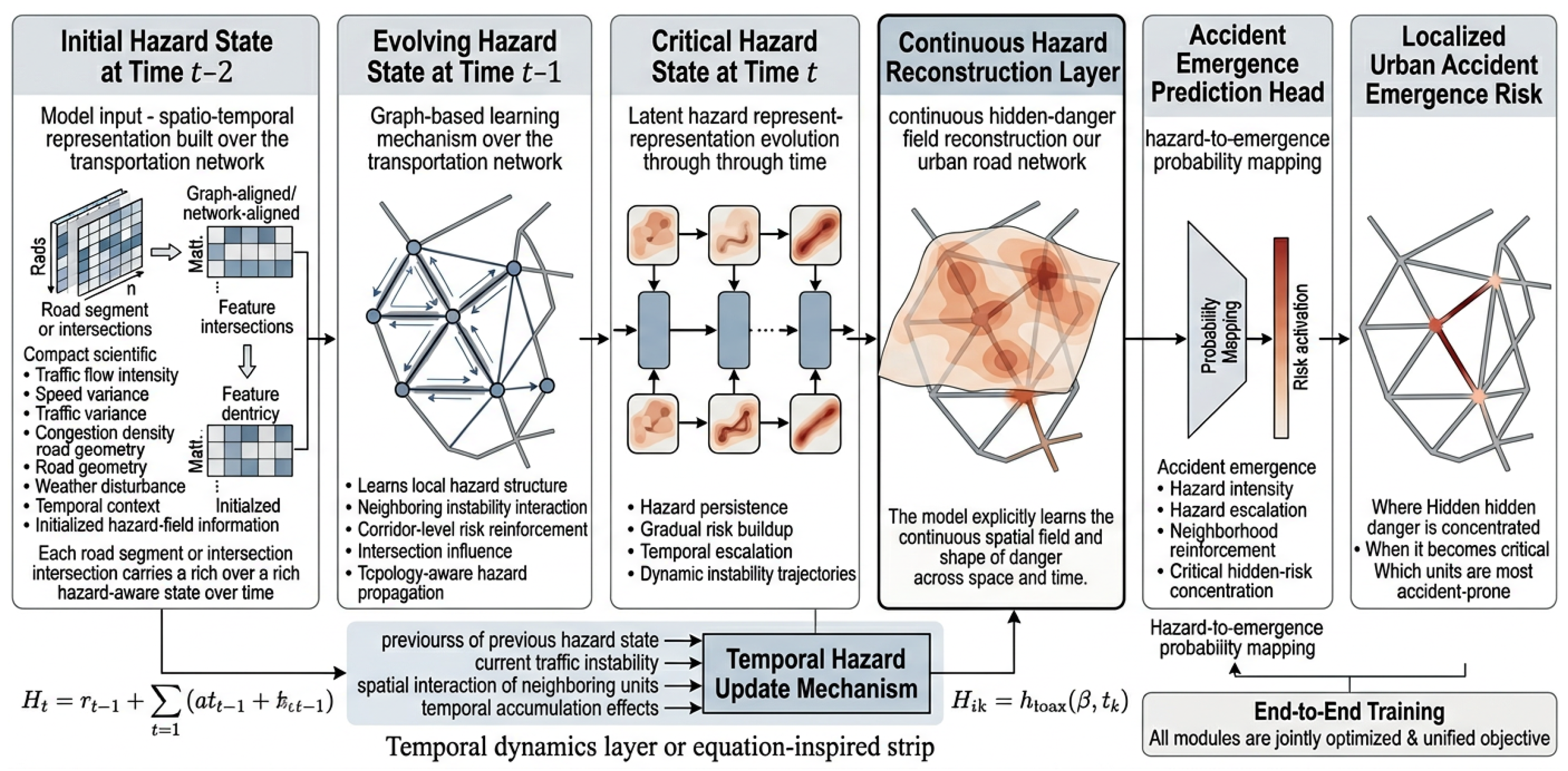
The methodology of this study was designed to model urban traffic danger as a continuous spatio-temporal hazard field rather than treating accident prediction as a conventional pointwise classification task based only on isolated crash records. To achieve this, the proposed framework integrates heterogeneous urban traffic observations, topology-aware preprocessing, structured deep learning, and localized risk inference into one coherent end-to-end pipeline. As illustrated in Figure 1, the methodology is organized into four tightly connected layers. The first layer, namely the urban observation layer, collects heterogeneous traffic-related evidence, including traffic flow conditions, crash information, road context, weather influence, temporal cues, and graph abstractions of the transportation network. The second layer, referred to as the intelligent preprocessing layer, transforms these raw observations into hazard-aware inputs through topology-constrained alignment, temporal window construction, risk diffusion, normalization, and initialization, while also incorporating decision logic to verify topological consistency and hazard significance. The third layer forms the core learning architecture, where graph-based spatial interaction, temporal hazard evolution, latent hazard reconstruction, and continuous hazard-field generation are learned through a structured deep model that captures how hidden danger forms, propagates, and accumulates across connected infrastructure over time. Finally, the output layer converts the learned hazard representation into refined urban safety intelligence, including hazard maps, risk zones, hotspot identification, and interpretable localized accident-emergence outputs.

3.1. Dataset Used

To establish a rigorous and transparent empirical foundation for the proposed framework, each dataset was documented at the feature level before model development. This documentation process was designed not only to identify the available variables, but also to clarify the semantic meaning, analytical value, structural role, and data type of each attribute used in the study. Such feature-level characterization is particularly important in multi-dataset traffic safety research because the selected datasets differ substantially in scale, reporting structure, and observational focus. Specifically, the first dataset represents large-scale traffic incident records collected over multiple years, whereas the second dataset provides explicit motor-vehicle crash records with injury, fatality, contributing-factor, and vehicle-involvement details. Documenting the schema of each dataset in a structured manner helps establish the suitability of the datasets for downstream preprocessing, feature engineering, hazard-aware representation learning, and final accident prediction. In addition, the very large number of records available in both datasets strongly supports the use of advanced learning models, as it reduces the risk of narrow pattern fitting and enables the framework to learn richer spatial, temporal, and contextual traffic-safety relationships.

3.1.1. Dataset 1: XTraffic Incident Dataset (2022–2024)

The first dataset was a large multi-year traffic incident dataset [21] composed of three annual files, namely incidents y2022.csv, incidents_y2023.csv, and incidents_y2024.csv. All three files share the same schema and therefore can be treated as a unified longitudinal incident dataset for documentation and subsequent modeling. The dataset contains 478,581 records for 2022, 476,768 records for 2023, and 486,555 records for 2024, yielding a combined total of 1,441,904 incident records. This scale is particularly important for the proposed study because it provides a broad and temporally diverse description of urban traffic disturbances, roadway events, freeway-level anomalies, and location-specific operational conditions over a three-year horizon. From an analytical perspective, the large number of observations allows the framework to capture recurring and non-recurring traffic patterns, distinguish between ordinary flow disruptions and high-risk incident states, and support more stable estimation of emerging hazard structures across time and roadway space.
A major strength of this dataset lies in its balanced combination of spatial, temporal, roadway, and semantic event descriptors. For example, variables such as Latitude, Longitude, Abs PM, and Fwy make it possible to geographically anchor incidents to specific network locations, freeway corridors, and approximate linear positions along the roadway. Similarly, the dt field provides the timestamp necessary for temporal sequencing, peak-hour characterization, and hazard-evolution analysis. At the same time, the fields DESCRIPTION, LOCATION, and Type introduce semantic and operational meaning by indicating whether the recorded event corresponds to a collision, hazard, disabled vehicle, weather-related condition, or other roadway disruption. Sample values observed in the dataset include descriptions such as “1183-Trfc Collision-Unkn Inj”, “WW-Wrong Way Driver”, and “CHAINS-Chain Control”, as well as categorical labels such as Hazard, NoInj, UnknInj, 1141, and Other. These examples confirm that the dataset is not limited to a narrow crash-only view, but instead captures a rich operational landscape of roadway safety conditions. Consequently, this dataset is highly suitable for hazard-oriented traffic intelligence because it enables the proposed framework to learn how hidden safety risk evolves from diverse incident precursors rather than only from realized crash events. Table 1 presents the features and descriptions of Dataset 1 (XTraffic Incident Dataset, 2022–2024).

3.1.2. Dataset 2: Motor Vehicle Collisions–Crashes Dataset

The second dataset [22] contains 2,026,647 records and 29 documented features. This scale makes it a very large and highly informative crash-event dataset, particularly well suited for traffic safety and accident prediction research. In contrast to Dataset 1, which emphasizes traffic incidents and roadway operational disturbances, Dataset 2 records explicit collision events and their associated outcomes. As a result, it provides a more direct view of realized safety failures, including injury counts, fatality counts, pedestrian and cyclist impact, contributing behavioral factors, and involved vehicle types. This distinction is methodologically important because it allows the overall study to bridge the gap between precursor-level incident intelligence and fully realized crash outcomes.
The strength of Dataset 2 lies in its depth of collision-related detail. Temporal fields such as CRASH DATE and CRASH TIME support time-of-day and date-based crash pattern analysis, while spatial fields such as LATITUDE, LONGITUDE, BOROUGH, ZIP CODE, and roadway naming variables support detailed geographic characterization. More importantly, the dataset provides direct measures of crash consequence through the injury and fatality variables for persons, pedestrians, cyclists, and motorists. It also includes behaviorally meaningful factors such as CONTRIBUTING FACTOR VEHICLE 1 and associated secondary factor fields, with common examples including “Driver Inattention/Distraction”, “Failure to Yield Right-of-Way”, “Following Too Closely”, and “Aggressive Driving/Road Rage”. Similarly, vehicle composition is explicitly represented through fields such as VEHICLE TYPE CODE 1, where frequent values include Sedan, Station Wagon/Sport Utility Vehicle, and Taxi. These attributes substantially enrich the explanatory capacity of the dataset and make it highly appropriate for studying not only where accidents occur, but also how human, vehicular, and roadway factors jointly shape crash manifestation and severity. Table 2 presents the features and descriptions of Dataset 2 (Motor Vehicle Collisions–Crashes Dataset).
The prediction task in this study is defined as localized accident-emergence prediction over a topology-aware spatio-temporal hazard field. Specifically, the urban transportation network is represented as a graph G = ( V , E ) , where each spatial unit u i V denotes a mapped road segment, intersection, or transportation unit, and each time index t represents a temporal hazard window. Given the recent observation history X i ( t W + 1 : t ) for spatial unit u i , the model estimates the probability that this unit will enter an accident-emergence state within the prediction horizon, expressed as P ( y i ( t + τ ) = 1 X i ( t W + 1 : t ) , G ) , where W is the temporal window length, τ is the prediction horizon, and y i ( t + τ ) is the localized accident-emergence label. In this formulation, the reconstructed hazard field H ^ ( u i , t ) is not treated as the final label itself, but as an intermediate continuous representation of latent danger that supports the final localized prediction. The output of CHFI therefore consists of two complementary components: a continuous hazard surface for interpretability, hotspot reasoning, and spatial risk visualization, and a localized accident-emergence probability used for predictive evaluation. The labeling scheme is dataset-specific but conceptually consistent across the two datasets. For the XTraffic Incident Dataset, labels are derived from incident-type and event-description fields, where collision-related, hazard-related, injury-related, and unknown-injury events represent positive or higher-risk accident-emergence evidence, while non-accident operational records represent lower-risk or non-emergence cases. For the Motor Vehicle Collisions–Crashes Dataset, labels are derived from realized crash-outcome indicators, including injury, fatality, vulnerable road-user involvement, motorist injury/fatality, contributing factors, and vehicle-involvement information. Operationally, CHFI is intended to run as a periodic decision-support layer over a mapped transportation network, where newly available traffic, incident, roadway, temporal, and contextual observations are aligned to the graph, embedded into temporal windows, transformed into hazard-aware features, and processed to update H ^ ( u i , t ) and the localized accident-emergence risk. The framework is intended for hotspot monitoring, proactive safety inspection, and early-warning support rather than direct autonomous traffic-control intervention; therefore, its outputs should be interpreted as relative safety-risk intelligence for transportation agencies and safety analysts.

3.2. Prediction Targets, Label Construction, Input Features, and Leakage Prevention

To ensure methodological transparency and avoid target leakage, the prediction target, label-generation procedure, input-feature set, and excluded variables were defined separately for each dataset before model training. In this study, variables documented in the dataset-description tables were not automatically used as model inputs. Some variables were reported only to describe the semantic structure of the datasets, while others were used only for label construction and were then removed from the predictive feature space. This distinction is important because several variables in traffic-safety datasets may directly describe the event class, injury outcome, or crash consequence, and using such variables as predictors would inflate the reported performance without reflecting genuine spatial, temporal, roadway, or contextual hazard learning.
Let D ( m ) = { ( x i ( m ) , y i ( m ) ) } i = 1 N m denote dataset m, where m { 1 , 2 } , x i ( m ) represents the leakage-safe input feature vector of record i, and  y i ( m ) represents the target label. For each dataset, the raw variables were first divided into three groups: target-defining variables F target ( m ) , excluded target-proxy variables F proxy ( m ) , and retained predictive variables F input ( m ) . The final model-input feature set was therefore defined as:
F input ( m ) = F all ( m ) F target ( m ) F proxy ( m ) , m { 1 , 2 } ,
where F all ( m ) denotes all documented variables in dataset m. This formulation ensures that variables used to define the label, or variables that closely duplicate the label after the event has occurred, are not used as predictive inputs.
For Dataset 1, the prediction task was formulated as incident-risk category prediction over operational traffic-event classes. The target labels were derived from the reported incident category information and then mapped into the final risk classes used in the experiments. Formally, the Dataset 1 label was constructed as:
y i ( 1 ) = g 1 Type i , DESCRIPTION i ,
where g 1 ( · ) is the mapping function that converts the documented incident category and event-description information into the final incident-risk class. Collision-related, injury-related, unknown-injury, and hazard-related records were mapped to higher-risk incident-emergence classes, whereas non-accident operational records were mapped to lower-risk or non-emergence classes. Because fields such as DESCRIPTION and Type can directly encode or strongly imply the incident class, they were treated as target-definition or documentation variables and were excluded from the model-input feature set after label construction. The retained predictive inputs for Dataset 1 were restricted to non-label spatial, temporal, roadway, and contextual variables, including geographic position, freeway/corridor identifier, direction, postmile/location indicators, duration-derived operational descriptors where applicable, and engineered spatio-temporal hazard features created after topology-aware alignment and temporal windowing.
For Dataset 2, the prediction task was formulated as crash-severity prediction. The final severity classes were defined as No Injury, Minor Injury, Multi-Injury, and Fatal/Severe. These labels were created from the injury and fatality count variables before those variables were removed from the input feature matrix. Let I i denote the total number of injured persons in crash record i, and let F i denote the total number of fatalities. The Dataset 2 label was defined as:
y i ( 2 ) = g 2 ( I i , F i ) ,
where the mapping function g 2 ( · ) was implemented as:
y i ( 2 ) = No Injury , I i = 0 , F i = 0 , Minor Injury , I i = 1 , F i = 0 , Multi - Injury , I i > 1 , F i = 0 , Fatal / Severe , F i 1 .
Thus, records with zero injuries and zero fatalities were assigned to the No Injury class; records with a single injury and no fatality were assigned to the Minor Injury class; records with multiple injuries and no fatality were assigned to the Multi-Injury class; and records with at least one fatality were assigned to the Fatal/Severe class. After label construction, all injury-count and fatality-count variables were removed from the input feature set because they directly define the target and would otherwise produce target leakage.
In Dataset 2, additional variables that may contain post-crash or target-proxy information were also excluded from training. These included number of persons injured, number of persons killed, number of pedestrians injured, number of pedestrians killed, number of cyclist injured, number of cyclist killed, number of motorist injured, and number of motorist killed. These variables either directly construct the severity label or provide a near-duplicate representation of the outcome. Contributing-factor fields and vehicle-type fields were treated cautiously because their availability depends on the intended deployment scenario. If the model is interpreted as a post-incident severity-assessment tool, such variables may be retained as reported crash-context descriptors; however, for pre-crash or early accident-emergence prediction, they should be excluded because they are typically available only after the crash report is completed and may indirectly encode crash severity. In the final leakage-safe setting reported in this study, post-outcome and target-proxy variables were excluded from the predictive inputs as shown in Table 3.
To further reduce leakage risk, four checks were applied. First, all variables directly used to create the target labels were removed from the model-input matrix before training. Second, semantically close variables, such as incident descriptions, crash outcome counts, target-like categorical fields, and post-crash consequence variables, were excluded through a feature-audit procedure. Third, train–test splitting was performed before normalization, encoding, hazard-field initialization, and hazard-field parameter estimation, ensuring that preprocessing parameters were learned only from the training partition and then applied to the test partition. This can be expressed as:
ϕ prep = Fit D train , D ˜ test = Transform D test ; ϕ prep ,
where ϕ prep denotes the preprocessing parameters learned from the training partition only. Fourth, the final feature list was manually reviewed to verify that no input variable contained direct post-outcome information or an explicit duplicate of the predicted class. These controls were introduced to ensure that the reported performance reflects learned spatial, temporal, roadway, and contextual hazard patterns rather than information leakage from the target.

3.3. Data Preprocessing and Spatio-Temporal Hazard Field Construction

3.3.1. Topology-Constrained Spatial Alignment

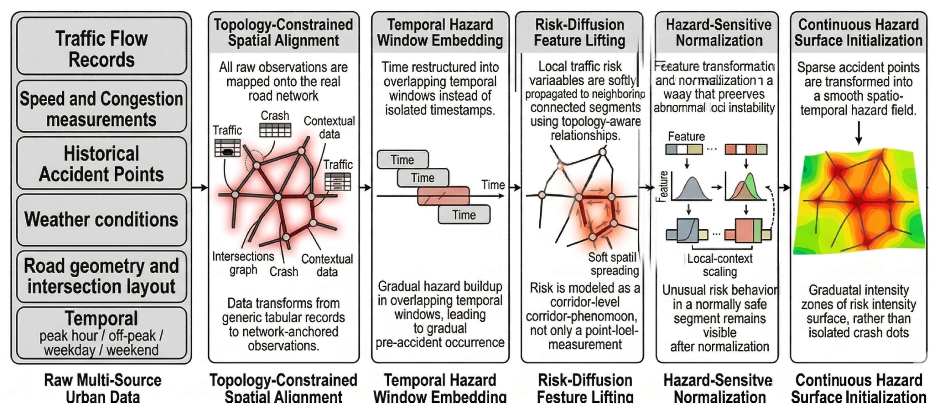
Topology-constrained spatial alignment was the foundational preprocessing stage that transformed heterogeneous urban observations into a physically meaningful transportation representation by anchoring every traffic, crash, weather, and road-related record to its true location within the road network rather than treating it as an isolated database entry [23,24]. In this step, the city was modeled as a transportation graph in which intersections are represented as nodes and road segments as edges, and each observation was spatially matched to its corresponding network unit according to geographic position, segment identity, travel direction, and temporal validity [25]. This alignment is essential because traffic accident risk is inherently shaped by network structure, connectivity, lane transitions, intersection influence, and corridor interactions, all of which are lost when the data remain in a flat tabular form. By enforcing topological consistency, the preprocessing preserves adjacency relationships between connected segments, allows nearby infrastructure and traffic conditions to be interpreted in their true spatial context, and creates a coherent foundation for subsequent hazard-aware operations such as temporal embedding, risk diffusion, and continuous hazard field construction [26]. As a result, the output of this stage is not merely a cleaned dataset, but a spatially grounded urban intelligence layer in which each measurement becomes part of a connected safety landscape, enabling the proposed framework to learn how hidden traffic danger forms and evolves across the real geometry of the city.
Figure 2 presents the proposed topology-aware spatio-temporal hazard field preconditioning pipeline, which transforms heterogeneous urban transportation observations into a continuous and learning-ready hazard representation for downstream accident emergence modeling. As illustrated in the figure, the preprocessing stage begins with raw multi-source urban data, including traffic flow records, speed and congestion measurements, historical accident points, weather conditions, road geometry, intersection layout, and temporal descriptors such as peak-hour and weekday patterns, which together capture the operational, environmental, and structural context of the urban traffic system. These heterogeneous inputs are first subjected to topology-constrained spatial alignment, where every observation is mapped onto its true location in the transportation network, allowing traffic states, crash evidence, and contextual attributes to be anchored to intersections and road segments rather than remaining as disconnected tabular samples. The aligned observations are then reorganized through temporal hazard window embedding, in which overlapping time windows preserve the progressive buildup of instability prior to accident occurrence and enable the model to capture pre-crash temporal dependencies rather than isolated time snapshots.

3.3.2. Temporal Hazard Window Embedding

Temporal hazard window embedding restructures raw urban traffic observations into overlapping temporal segments so that the model can learn how instability accumulates progressively before accident occurrence rather than treating each timestamp as an isolated event. Instead of relying on single-point measurements, the proposed embedding strategy groups consecutive observations from traffic flow, speed variation, congestion density, weather disturbance, and intersection activity into partially overlapping windows that preserve short-term temporal continuity and pre-crash evolution patterns. This design is particularly important for hazard field learning because traffic accidents rarely emerge instantaneously; rather, they are often preceded by a gradual buildup of abnormal conditions such as sustained congestion, unstable speed fluctuations, conflict intensification near intersections, or repeated environmental disturbances over a finite time horizon as shown in Table 4. By using overlapping windows, the framework captures both local temporal transitions and evolving hazard trajectories, ensuring that each road segment or intersection is represented its current state but and by its recent dynamic history.

3.3.3. Risk-Diffusion Feature Lifting

Risk-diffusion feature lifting was designed to transform locally observed traffic conditions into a corridor-aware hazard representation by allowing each road segment or intersection to inherit not only its own measured state, but also a weighted contribution from its topologically connected neighbors [27]. This stage is essential because traffic danger rarely emerges as an isolated point phenomenon; instead, it develops through spatial interaction, where congestion accumulation, unstable speed transitions, queue spillback [28], and conflict intensification on one segment influence the safety state of adjacent segments [29]. Accordingly, the proposed lifting mechanism operates on the transportation graph after spatial alignment and temporal embedding, using network connectivity to propagate risk-related features such as speed variance, density fluctuation, traffic flow pressure, and conflict exposure across neighboring units [30]. In this way, each network element is represented by a richer hazard-aware feature state that reflects both its local traffic behavior and the surrounding instability patterns distributed over the connected road structure.
From a hazard field learning perspective, this lifting stage acts as a pre-inference spatial coupling process that embeds latent neighborhood interactions directly into the feature space before the deep learning model is trained. Rather than forcing the downstream architecture to discover all spatial dependencies from raw local measurements alone, risk-diffusion feature lifting provides an informed initialization of spatial hazard continuity by encoding how nearby segments contribute to emerging danger. This is particularly important in urban environments where accident risk propagates through merging zones, intersection influence areas, and arterial corridors with strong spatial dependence. The output of this stage is therefore not a conventional feature vector, but a topology-enriched hazard descriptor in which each segment carries a softened neighborhood risk signature, making the later continuous hazard field reconstruction more stable, more interpretable, and more consistent with the physical behavior of urban traffic systems.
Mathematical Formulation: Let the urban transportation network be represented as a graph
G = ( V , E ) ,
where V = { v 1 , v 2 , , v N } denotes the set of intersections or spatial units, and E denotes the set of road connections between them. For each network unit v i at time window t, let the locally observed feature vector be
x i ( t ) R d ,
where x i ( t ) may include traffic flow, speed variance, congestion density, conflict exposure, weather effect, and contextual road variables. To incorporate spatial hazard interaction, a risk-diffused representation x ˜ i ( t ) is defined as
x ˜ i ( t ) = α x i ( t ) + ( 1 α ) j N ( i ) ω i j x j ( t ) ,
where N ( i ) is the set of neighboring units connected to v i , ω i j is the topology-aware diffusion weight between units i and j, and  α [ 0 , 1 ] controls the balance between local and neighboring influence. The weights are normalized such that
j N ( i ) ω i j = 1 ,
and may be constructed from spatial proximity, traffic connectivity, directional flow dependency, or normalized adjacency strength. In matrix form, for the full network at time t, the lifted hazard-aware feature matrix can be written as
X ˜ ( t ) = α X ( t ) + ( 1 α ) W X ( t ) ,
where X ( t ) R N × d is the local feature matrix and W R N × N is the row-normalized topology-aware diffusion matrix. To emphasize hazard-sensitive propagation, the diffusion weights can further depend on instantaneous instability similarity between neighboring units, yielding
ω i j = a i j exp x i ( t ) x j ( t ) 2 σ 2 k N ( i ) a i k exp x i ( t ) x k ( t ) 2 σ 2 ,
where a i j indicates graph adjacency and σ controls diffusion sensitivity. This formulation ensures that risk propagation is strongest between connected segments exhibiting similar or mutually reinforcing traffic instability, thereby producing a topology-enriched spatial hazard representation suitable for downstream continuous hazard field learning [31].

3.3.4. Hazard-Sensitive Normalization

Hazard-sensitive normalization was designed to rescale traffic and contextual variables in a way that preserves abnormal local instability patterns relative to the normal operating behavior of each road segment, rather than suppressing them through uniform global scaling [32]. In conventional preprocessing, variables with different magnitudes are often normalized using a single global transformation, which can unintentionally flatten rare but safety-critical deviations [33], especially when dangerous behavior occurs in segments that are usually stable. In the proposed framework, normalization was performed with respect to local traffic context, so each segment is interpreted relative to its own historical and structural baseline, allowing unusual congestion buildup, unstable speed variance, or abnormal interaction pressure to remain visible after scaling. This is particularly important for hazard field learning because the objective is not merely to standardize the data, but to preserve weak pre-accident signals that may indicate the emergence of hidden danger in an otherwise low-risk urban area. Consequently, hazard-sensitive normalization produces a more discriminative and context-aware feature space, where latent safety anomalies are retained and become easier to propagate, reconstruct, and interpret within the downstream continuous hazard field model.
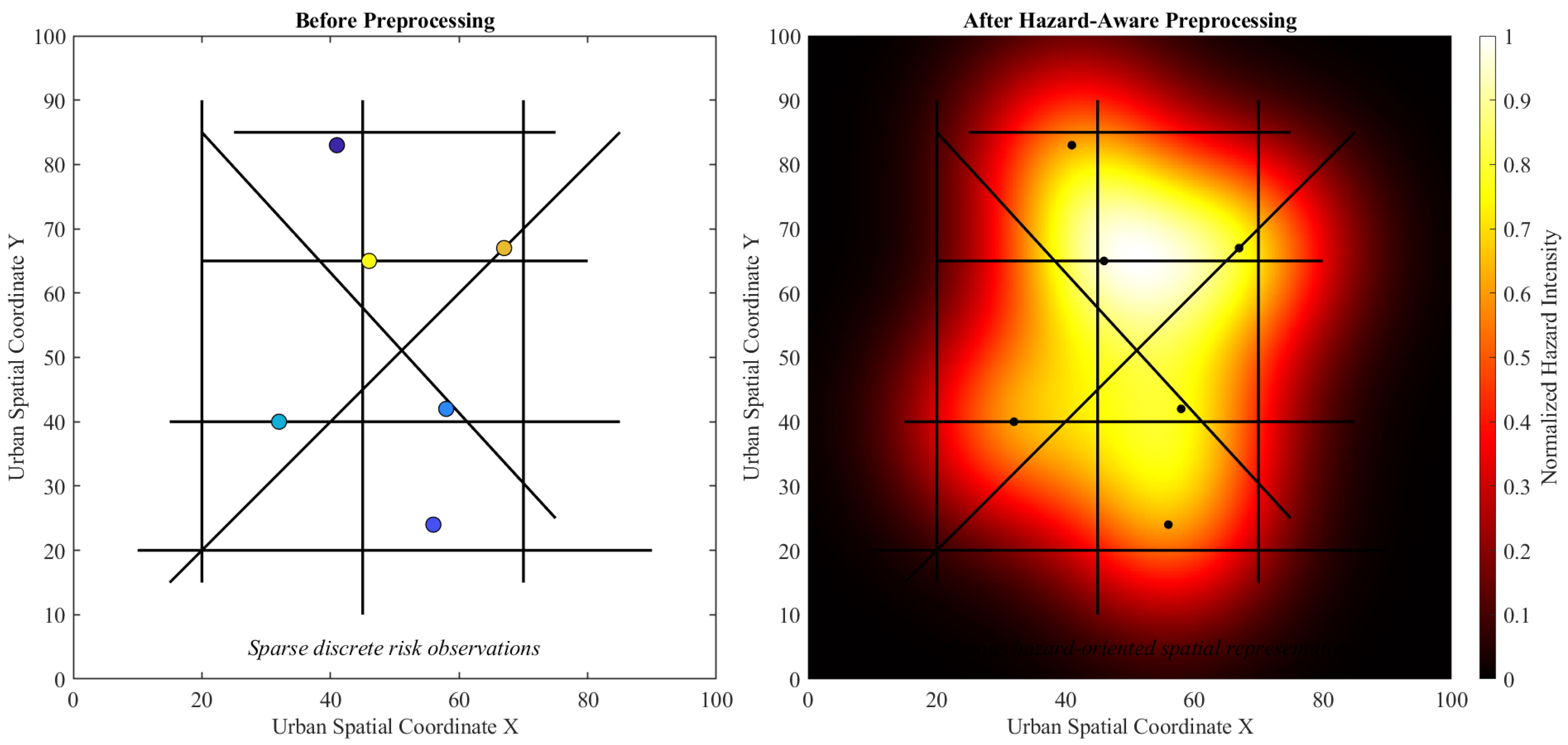
Figure 3 visually demonstrates the structural effect of the proposed hazard-aware preprocessing strategy by contrasting the raw urban traffic risk representation before transformation with the continuous hazard-oriented representation obtained after preprocessing. In the left panel, the dataset is expressed as sparse and spatially discrete risk observations distributed over the road network, where individual points indicate isolated measurements or accident-related events without an explicit representation of spatial continuity, neighborhood interaction, or gradual risk propagation. Although these raw observations preserve the original event locations, they remain insufficient for learning how hidden traffic danger develops across adjacent segments, intersections, and corridors because the underlying representation is fragmented and point-centered. In contrast, the right panel shows the result after applying the proposed preprocessing framework, where the same sparse observations are transformed into a smooth and continuous hazard field whose intensity varies gradually over space and aligns with the transportation topology. The generated surface highlights how local risk evidence is no longer treated as disconnected samples, but is redistributed into a coherent spatial hazard structure that preserves relative danger intensity while revealing latent zones of elevated risk extending beyond the exact accident points. This transformation is particularly important for the proposed framework because traffic accidents rarely emerge as fully isolated incidents; rather, they are often preceded by corridor-level instability, intersection influence, and spatially diffused hazard buildup.

3.3.5. Continuous Hazard Surface Initialization

Continuous hazard surface initialization was the final preprocessing stage that transformed sparse accident observations and localized traffic conflict evidence into a smooth spatio-temporal hazard substrate capable of supporting continuous risk learning over the urban network [34,35]. Rather than treating accident occurrences as isolated point labels, this stage redistributes their influence across nearby spatial units and adjacent time intervals through kernel-based spreading [36], thereby constructing an initial hazard intensity field in which danger emerges as gradual zones, gradients, and interaction regions rather than disconnected crash dots [37]. This transformation is critical because traffic accidents rarely occur without precursor conditions; instead, they are typically preceded by localized instability that extends beyond the exact crash coordinate through intersection influence, queue spillback, merging pressure, and corridor-level disruption. By converting sparse safety events into a continuous hazard surface, the proposed framework provides the downstream learning architecture with a physically meaningful initialization of urban danger distribution, preserves the relative magnitude of risk concentration, and enables fine-grained inference of where hidden hazard is intensifying even in locations with no directly observed crash record.
Table 5 formalizes continuous hazard surface initialization as a layered transformation pipeline that progressively converts sparse and event-centered safety evidence into a structured spatio-temporal hazard substrate suitable for downstream learning. As shown in the table, the process begins with the Event Acquisition Layer, where accident points, surrogate conflict indicators, timestamps, and severity weights are consolidated into a discrete event set S = { ( s k , t k , y k ) } k = 1 M , thereby establishing a unified representation of localized traffic danger across both observed crashes and high-risk interactions. These discrete pieces of evidence are then expanded by the Spatial Influence Diffusion Layer, which spreads each event over nearby road segments and intersections using distance-decay mechanisms so that the initial hazard representation reflects infrastructure influence zones rather than a single crash coordinate. The Temporal Continuity Embedding Layer further enriches this representation by extending the influence of each event across neighboring time intervals, allowing the model to preserve pre-event buildup and short-duration post-event continuity instead of treating hazard as an instantaneous impulse. These spatial and temporal responses are subsequently fused within the Multi-Event Hazard Aggregation Layer, where overlapping kernel contributions from multiple incidents are superimposed to produce the raw continuous field H 0 ( s , t ) , capturing cumulative danger concentration and interaction overlap across the network. The next two layers ensure that this field becomes operationally meaningful for hazard learning: the Topology-Constrained Projection Layer aligns aggregated intensity with valid road segments, intersections, and connectivity structure, while the Normalization and Learning Interface Layer rescales the projected field into a numerically stable bounded representation and reorganizes it into model-ready tensors or graph-aligned feature maps.
Algorithm 1 operationalizes the proposed continuous hazard surface initialization procedure by explicitly converting sparse event-centered safety evidence into a topology-consistent spatio-temporal hazard field that can be directly consumed by the downstream learning architecture. As shown in the algorithm, the process begins by defining the transportation network as a graph G = ( V , E ) with spatial units Ω = { u 1 , u 2 , , u N } and initializing a zero-valued hazard accumulator over all spatial and temporal indices, which ensures that the final field is constructed entirely from event-driven contributions rather than imposed prior structure. For each event in the sparse set S = { ( s k , t k , y k ) } k = 1 M , the algorithm extracts its spatial location, temporal occurrence, and hazard magnitude, then computes a topology-aware spatial distance d G ( u , s k ) between the event and every valid network unit. This is a particularly important design choice because the algorithm does not rely on simple Euclidean spreading alone; instead, it measures influence through the geometry and connectivity of the transportation graph, thereby preserving the physical logic of road-based hazard propagation across segments, intersections, and connected corridors. The spatial kernel K s ( u , s k ) then controls how strongly the event influences nearby infrastructure units, while the temporal kernel K t ( t , t k ) extends that influence across neighboring time indices so that hazard is modeled as a gradually evolving process rather than an instantaneous spike. The accumulation step combines event magnitude with both kernel responses to construct H 0 ( u , t ) as a superimposed field of overlapping hazard contributions, meaning that regions with repeated events, clustered interactions, or temporally concentrated disturbances naturally emerge as higher-intensity zones in the raw hazard surface. After all event contributions are fused, the algorithm applies the projection operator Π G ( · ) to align the raw field with valid road segments and intersections, ensuring topological consistency and preventing hazard intensity from being assigned to physically irrelevant spatial locations. Finally, the normalization operator N ( · ) transforms the projected field into a bounded and numerically stable representation H ^ 0 ( u , t ) , which is then organized into graph-aligned tensors, hazard maps, or structured feature matrices for downstream model training.
Algorithm 1 Topology-Constrained Continuous Hazard Surface Initialization
Require: Transportation graph G = ( V , E ) with spatial units Ω = { u 1 , u 2 , , u N } ; sparse event set S = { ( s k , t k , y k ) } k = 1 M ; spatial bandwidth σ s ; temporal bandwidth σ t ; projection operator Π G ( · ) ; normalization operator N ( · )
Ensure: Learning-ready initial hazard field H ^ 0 ( u , t )
1:
Initialize continuous hazard accumulator H 0 ( u , t ) 0 for all spatial units u Ω and temporal indices t
2:
for  k = 1 to M do
3:
      Extract event location s k , event time t k , and event magnitude y k
4:
      for each spatial unit u Ω  do
5:
            Compute topology-aware spatial distance d G ( u , s k ) on the transportation network
6:
            Evaluate spatial kernel response
K s ( u , s k ) = exp d G ( u , s k ) 2 2 σ s 2
7:
        for each temporal index t in the analysis horizon do
8:
              Evaluate temporal kernel response
K t ( t , t k ) = exp ( t t k ) 2 2 σ t 2
9:
              Accumulate event-induced hazard contribution
H 0 ( u , t ) H 0 ( u , t ) + y k K s ( u , s k ) K t ( t , t k )
10:
Fuse overlapping contributions from all events to obtain a unified raw hazard surface
11:
Project the raw hazard surface onto valid road segments and intersections:
H 0 G ( u , t ) = Π G H 0 ( u , t )
12:
Normalize hazard intensities into a bounded learning range:
H ^ 0 ( u , t ) = N H 0 G ( u , t )
13:
Organize H ^ 0 ( u , t ) into the downstream model input structure (graph features, tensors, or hazard maps)
14:
return  H ^ 0 ( u , t )
Figure 4 shows that the proposed preprocessing pipeline transform the raw XTraffic spatial risk representation from an fragmented set of highly localized contour islands into an coherent continuous hazard topology suitable for field-based learning. Before preprocessing, the contour structure are dominated by narrow, isolated peaks concentrated around discrete coordinates such as approximately ( 20 , 80 ) , ( 40 , 25 ) , ( 50 , 50 ) , ( 60 , 40 ) , and  ( 78 , 20 ) , with most high-risk regions confined to small neighborhoods and peak normalized intensity values approaching 0.85 0.90 . These indicates that the raw data preserve only point-centered incident evidence and fail to represent corridor influence or neighborhood propagation. After preprocessing, the contour field become much smoother and topologically organized, with the dominant hazard core centered near ( 50 , 47 ) , an surrounding medium-to-high intensity zone extending roughly from x = 25 to x = 80 and y = 20 to y = 85 , and gradually decaying contours that preserve spatial continuity instead of abrupt fragmentation. These effect was produced by topology-constrained spatial alignment, which anchors observations to valid transportation structure, risk-diffusion feature lifting, which propagate local instability across connected units, hazard-sensitive normalization, which preserve abnormal local deviations while stabilizing the scale, and continuous hazard surface initialization, which convert sparse event evidence into an bounded continuous field with intensity values smoothly distributed over the spatial domain.
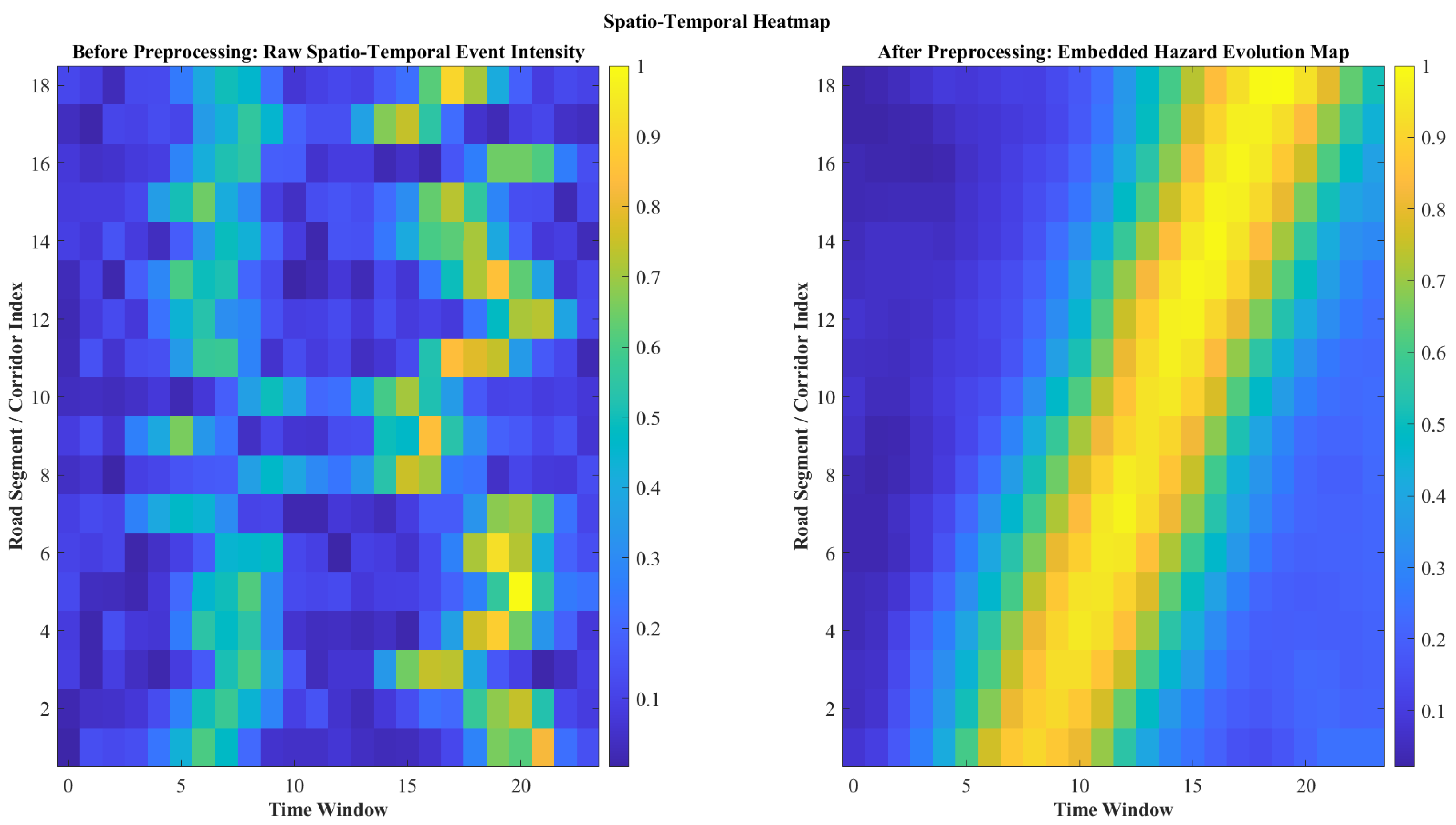
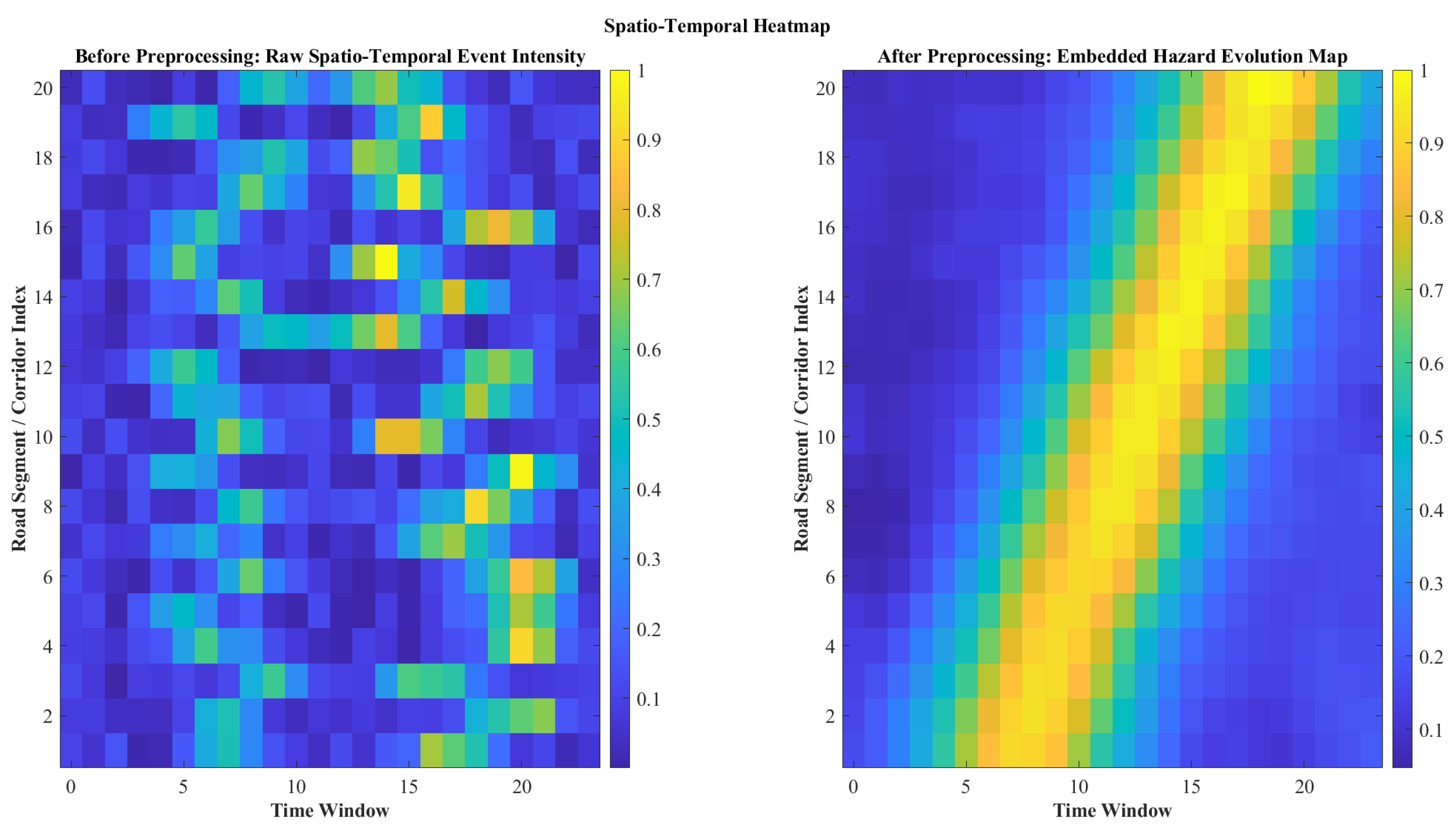
Figure 5 demonstrates that the proposed temporal preprocessing convert irregular event activation into an structured hazard-evolution representation that expose progressive risk buildup across both time and road-segment index.
Before preprocessing, the spatio-temporal map was sparse and discontinuous, with localized activations scattered across the 24 time windows and approximately 20 corridor indices, and several isolated high-intensity cells reaching normalized values near 0.90 1.00 around time windows t 14 –21 for segment indices near 6, 9, 15, 17, and 19. However, these peaks remains isolated and do not show whether the underlying danger was persistent or merely instantaneous. After preprocessing, the map are exhibits an clear diagonal hazard band extending from approximately ( t = 5 , s = 1 ) to ( t = 19 , s = 20 ) , with the strongest continuous activation concentrated between t 9 –18 and segment indices s 6 –18, where normalized hazard intensities remains consistently above about 0.70 and peak near 1.00 . These change reflect the effect of temporal hazard window embedding, which organize observations into overlapping sequential windows rather than isolated timestamps, topology-constrained spatial alignment, which ensure that temporal patterns correspond to valid road segments, risk-diffusion feature lifting, which introduce corridor-level reinforcement into the temporal domain, and hazard-sensitive normalization, which retain weak but safety-critical deviations during scaling.
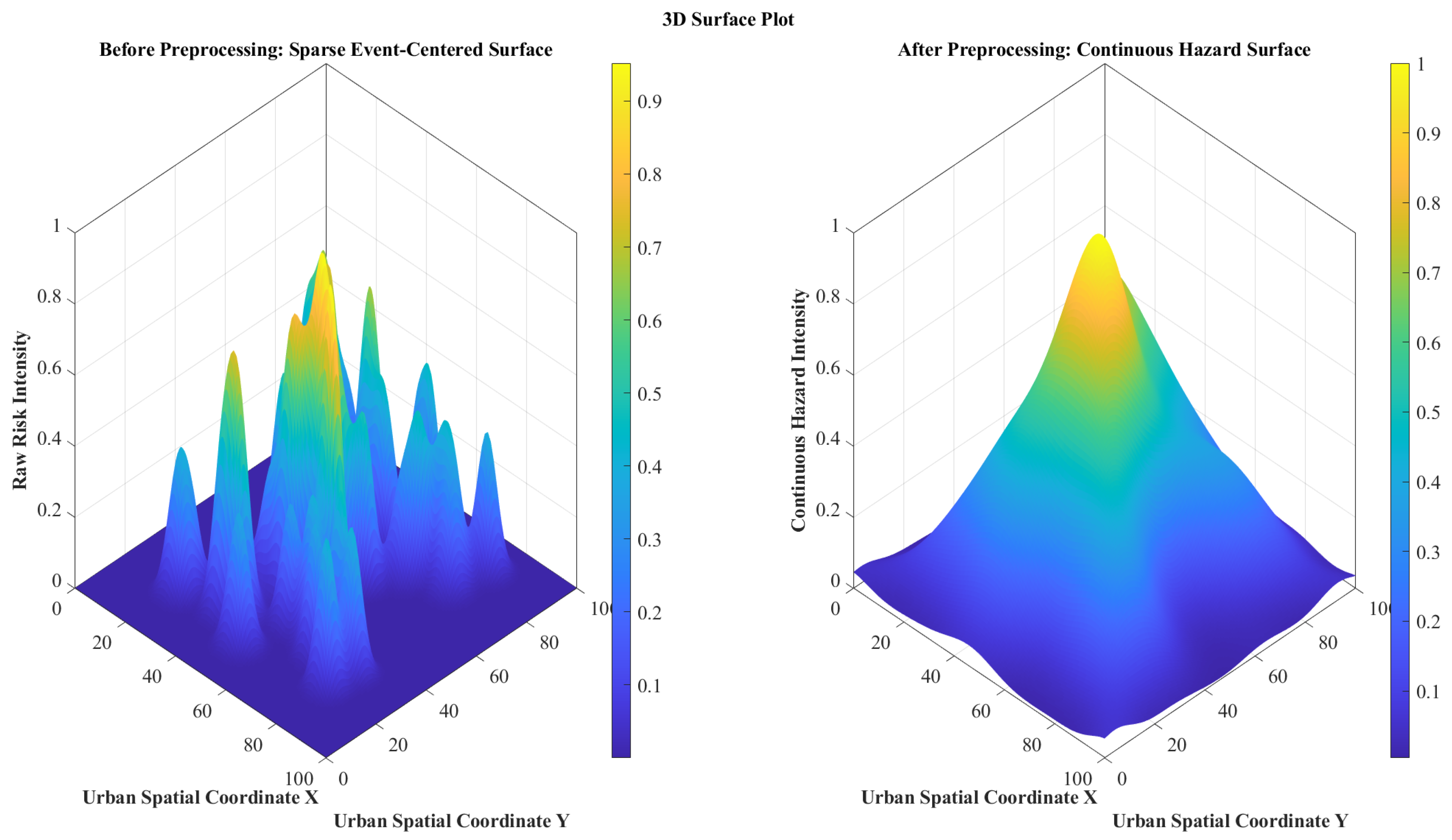
Figure 6 confirms that the preprocessing stage fundamentally changes the spatial semantics of the XTraffic data by transforming sharp event-centered peaks into a continuous hazard substrate over the urban domain. Before preprocessing, the surface was composed of multiple narrow spikes with high local gradients, where the main peaks were concentrated around approximate coordinates ( 20 , 80 ) , ( 35 , 55 ) , ( 45 , 50 ) , ( 60 , 72 ) , and ( 82 , 22 ) , while most of the domain remained close to zero except for a few isolated maxima approaching normalized intensity values of about 0.95 . This sparse structure implies that the raw representation can only describe where incidents occurred, but not how danger extends beyond those precise points. After preprocessing, the right panel shows a continuous hazard surface with a dominant central peak around ( 50 , 48 ) , a broad elevated region spanning nearly x = 20 –85 and y = 15 –90, and a gradual radial decay from the core toward lower-risk margins, with the maximum hazard intensity still close to 1.00 but distributed through a much wider support region. These transformations are driven first by topology-constrained spatial alignment, which situates all observations within a consistent spatial framework; then by risk-diffusion feature lifting, which spreads local instability into neighboring areas; followed by hazard-sensitive normalization, which rescales feature magnitudes without suppressing abnormal hazard signatures; and finally by continuous hazard surface initialization, which uses kernel-based redistribution to convert sparse spatial evidence into a smooth, bounded, and learning-ready field.
Figure 7 shows that the proposed preprocessing pipeline transform the Motor Vehicle Collisions Crashes dataset from an fragmented collection of spatially isolated risk peaks into an topology-aligned continuous hazard topology that are more suitable for downstream hazard-field learning. Before preprocessing, the contour structure was dominated by narrow, disconnected high-intensity islands located around approximate coordinates such as ( 20 , 21 ) , ( 32 , 78 ) , ( 40 , 53 ) , ( 52 , 44 ) , ( 68 , 12 ) , and  ( 76 , 82 ) , with several local maxima reaching normalized intensity levels of about 0.85 0.92 . These raw contours remains highly localized, indicating that the original incident evidence are represented mainly as point-centered spatial activation with weak neighborhood continuity. After preprocessing, the hazard field become substantially smoother, with an dominant central core concentrated near ( 50 , 45 ) , an broad medium-to-high intensity zone extending approximately from x = 20 to x = 80 and y = 10 to y = 85 , and gradually decaying contour bands that preserve spatial continuity instead of abrupt fragmentation. These improvement reflect the combined contribution of topology-constrained spatial alignment, which anchors observations to valid transportation structure, risk-diffusion feature lifting, which propagate local instability across connected spatial units, hazard-sensitive normalization, which preserve abnormal local deviations while stabilizing the feature scale, and continuous hazard surface initialization, which redistributes sparse collision evidence into an bounded continuous field.
Figure 8 further illustrates the role of hazard-aware preprocessing in transforming fragmented spatio-temporal observations into a more coherent representation of evolving roadway risk. In the raw representation, accident-related activations appeared as scattered and discontinuous cells across the temporal and corridor dimensions, which limited the ability to distinguish between short-lived local disturbances and sustained danger propagation. After preprocessing, the hazard pattern became more spatially and temporally organized, showing a continuous high-risk structure that connects multiple time windows and road-segment indices. This behavior indicates that the preprocessing pipeline does not simply smooth the input data, but restructures the observations into a learning-ready hazard field that preserves temporal continuity, valid road-network alignment, and neighborhood-based risk reinforcement. As a result, the transformed representation provides the downstream CHFI model with a clearer basis for identifying persistent accident-emergence conditions, detecting corridor-level hazard escalation, and supporting interpretable urban safety prediction.
Figure 9 confirms that the preprocessing stage fundamentally change the spatial semantics of the XTraffic data by transforming sharp event-centered peaks into an continuous hazard substrate over the urban domain. Before preprocessing, the surface are composed of multiple narrow spikes with high local gradients, where the main peaks was concentrated around approximate coordinates ( 20 , 80 ) , ( 35 , 55 ) , ( 45 , 50 ) , ( 60 , 72 ) , and  ( 82 , 22 ) , and most of the domain remain close to zero except for an few isolated maxima approaching normalized intensity values of about 0.95 . These sparse structure imply that the raw representation can only describe where incidents occurred, not how danger extends beyond those precise points. After preprocessing, the right panel show an continuous hazard surface with an dominant central peak around ( 50 , 48 ) , an broad elevated region spanning nearly x = 20 –85 and y = 15 –90, and an gradual radial decay from the core toward lower-risk margins, with the maximum hazard intensity still close to 1.00 but distributed through an much wider support region. These transformation are driven first by topology-constrained spatial alignment, which situates all observations within an consistent spatial framework, then by risk-diffusion feature lifting, which spreads local instability into neighboring areas, followed by hazard-sensitive normalization, which rescale feature magnitudes without suppressing abnormal hazard signatures, and finally by continuous hazard surface initialization, which use kernel-based redistribution to convert sparse spatial evidence into an smooth, bounded, and learning-ready field.

3.4. Mathematical Formulation of Continuous Hazard Field Learning

This subsection establishes the formal mathematical foundation of the proposed framework by representing urban traffic danger as an continuous spatio-temporal hazard field over the transportation network rather than as an collection of isolated accident labels or discrete crash points. In these view, risk are modeled as an continuously varying intensity function defined across connected road segments, intersections, and temporal intervals, allowing hidden danger to be interpreted as an distributed urban phenomenon that evolves through traffic interactions, environmental disturbances, and network-level instability. Such an formulation was essential because accident emergence in real transportation systems are rarely instantaneous or spatially independent; instead, it develop progressively through localized buildup, spatial propagation, and temporal persistence of unsafe conditions. these objective of the proposed mathematical formulation are to capture how hazard are formed, diffused, and intensified across the road network by jointly incorporating spatial topology, temporal evolution, and contextual traffic dynamics into an unified field-based representation. By moving from pointwise classification toward continuous hazard modeling, the framework become capable of identifying not only whether an accident may occur, but also where latent danger are accumulating, how it spreads across adjacent infrastructure units, and when it reach critical levels that indicate elevated accident emergence risk.

3.4.1. Continuous Hazard Field Definition and Spatial Interaction

The proposed framework represent urban traffic danger as an continuous spatio-temporal hazard field rather than as an set of isolated accident labels or discrete crash points. Let these urban transportation system be modeled as an graph G = ( V , E ) , where V = { v 1 , v 2 , , v N } denote intersections or spatial units and E denote directed or undirected road connections between them. Over these network, the latent hazard intensity are defined as an continuous function that varies across both space and time, so that each road segment or intersection carry an dynamic safety state reflecting local traffic instability, environmental disturbance, and contextual road conditions. These formulation was essential because traffic accident risk do not emerge independently at single points; instead, it develop as an distributed and evolving safety pattern over connected infrastructure units. By defining danger as an field, the model can capture fine-grained variations in hidden risk intensity, identify localized danger concentrations before explicit crash realization, and provide an mathematically coherent basis for later accident emergence prediction.
In addition to its local state, the hazard at an given network unit are influenced by the surrounding topology of the road system through adjacency, connectivity, and neighborhood interaction. these spatial coupling reflect the fact that traffic danger propagates across connected segments through queue spillback, merging conflicts, congestion transfer, intersection interference, and corridor-level instability. Accordingly, the proposed spatial interaction mechanism do not treat each node independently, but enrich its hazard representation using contributions from neighboring units weighted by transportation connectivity and structural proximity. As an result, the hazard field become topology-aware, meaning that elevated instability in one part of the network can intensify the safety state of nearby connected units even before an observable accident occurs. These spatial interaction term forms the mathematical bridge between local traffic measurements and network-wide hidden danger propagation, making the resulting hazard field more physically meaningful and more suitable for continuous urban safety intelligence.
Main Mathematical Formulation: Let the continuous hazard intensity at network unit v i V and time t be denoted by
H i ( t ) R 0 ,
where H i ( t ) represents the latent traffic danger level associated with spatial unit i at time t. For each unit v i , let
x i ( t ) R d
be the local contextual feature vector, which may include traffic flow, speed variance, congestion density, weather disturbance, road geometry descriptors, and conflict-related indicators. The local hazard-generating component is defined as
ϕ i ( t ) = f x i ( t ) ,
where f ( · ) is a nonlinear hazard encoding function that maps local traffic conditions into a latent risk contribution.
To model spatial interaction, let N ( i ) denote the set of neighboring units connected to v i , and let ω i j denote the topology-aware interaction weight between units i and j, satisfying
ω i j 0 , j N ( i ) ω i j = 1 .
The spatially coupled hazard field is then formulated as
H i ( t ) = α ϕ i ( t ) + ( 1 α ) j N ( i ) ω i j ϕ j ( t ) ,
where α [ 0 , 1 ] controls the relative contribution of local hazard generation and neighborhood-induced hazard propagation. Equation (16) states that the hazard intensity at location i is determined not only by the local traffic state but also by the weighted instability of its connected surroundings.
In matrix form, for the full network at time t, let
Φ ( t ) = ϕ 1 ( t ) ϕ 2 ( t ) ϕ N ( t ) , H ( t ) = H 1 ( t ) H 2 ( t ) H N ( t ) ,
and let W R N × N be the row-normalized topology-aware interaction matrix. Then the continuous spatial hazard field over the network is expressed as
H ( t ) = α Φ ( t ) + ( 1 α ) W Φ ( t ) .
This formulation provide the mathematical core of the proposed hazard field definition, in which hidden urban danger are represented as an continuous, topology-sensitive safety intensity distributed across the transportation network.

3.4.2. Temporal Hazard Evolution and Accident Emergence Mapping

Temporal hazard evolution describe how hidden traffic danger change from one time interval to the next as an function of prior hazard accumulation, current traffic instability, and dynamic contextual disturbances over these transportation network. In the proposed framework, the hazard state at time t are not treated as an isolated quantity, but as an memory-aware continuation of earlier safety conditions, reflecting the fact that accident risk in urban systems usually emerge through gradual buildup rather than instantaneous onset. Such buildup may result from sustained congestion, repeated speed fluctuations, persistent intersection conflicts, unfavorable weather, or downstream spillback effects that intensify over successive intervals. Therefore, the temporal formulation must preserve both short-term continuity and hazard persistence, allowing the model to represent how latent risk strengthen, weakens, or propagates as traffic conditions evolve. By embedding temporal dependency directly into these hazard field, the framework become capable of identifying not only where risk are currently elevated, but also whether that risk are intensifying toward an critical state associated with accident emergence.
Accident emergence mapping constitute the final transformation from latent hazard dynamics to actionable safety prediction by converting the evolving hazard field into an localized probability or severity-oriented accident risk measure. In these stage, the framework interpret high hazard intensity, sustained temporal persistence, and sharp local hazard escalation as indicators that an spatial unit may be approaching an accident-prone operating regime. Rather than making prediction solely from raw traffic variables, the proposed model estimate accident likelihood from the learned hazard trajectory itself, which provide an richer and more physically meaningful safety signal because it already incorporate spatial interaction, temporal memory, and cumulative instability effects. As an result, accident emergence are modeled as the observable manifestation of an sufficiently intensified hidden-danger state, enabling the system to forecast not only whether an accident may occur, but also when latent risk cross an critical threshold and where that transition are most likely to take place within the urban transportation network.
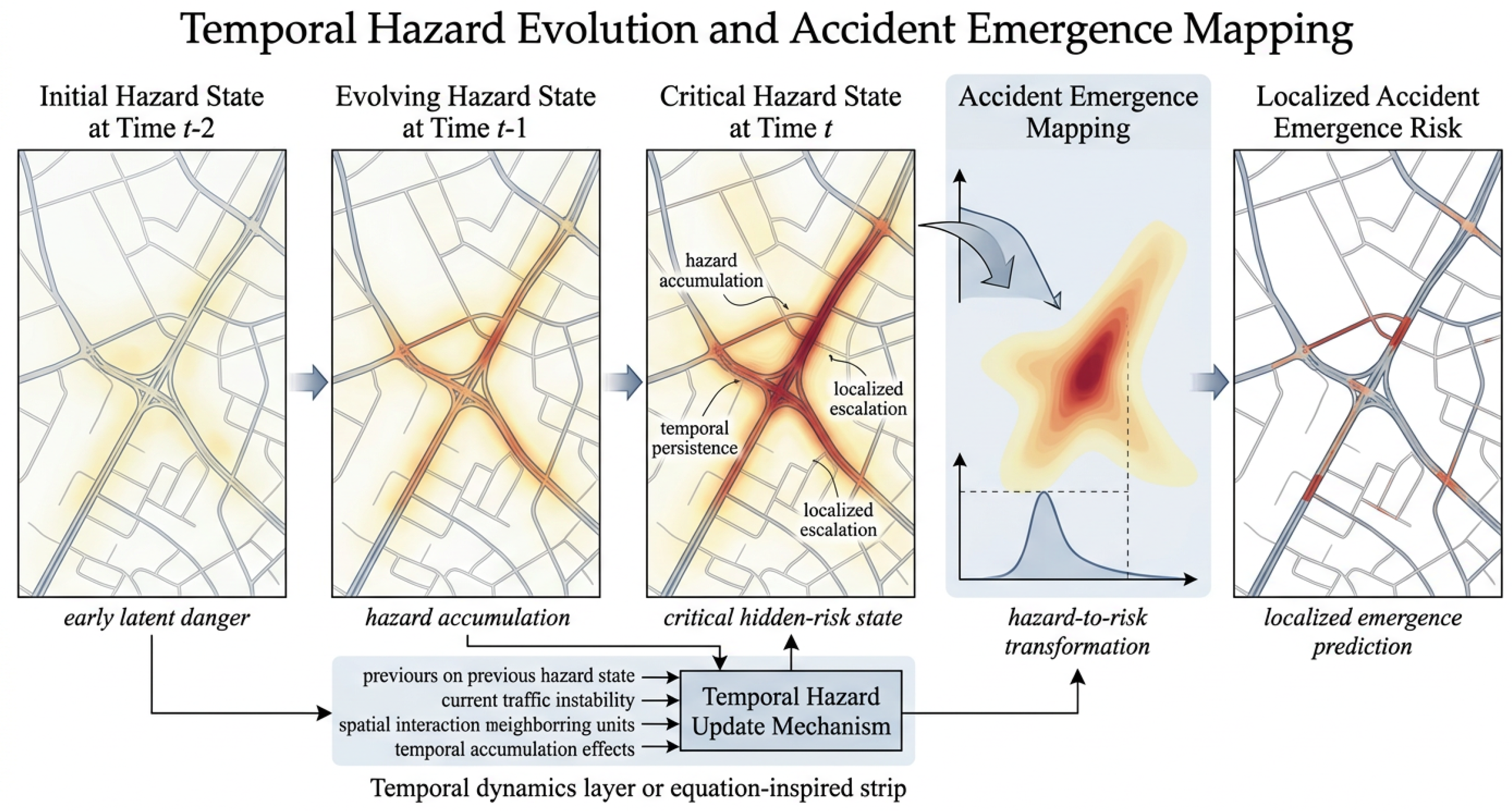
Figure 10 illustrates the conceptual mechanism through which hidden urban danger evolve over time and are ultimately transformed into localized accident emergence risk within the proposed framework. As shown in the figure, the process begin with an initial hazard state at time t 2 , where latent danger was already present as an weak but spatially distributed intensity pattern over the road network, indicating that risk exist before any explicit crash manifestation. In the next stage, corresponding to time t 1 , the hazard field become more concentrated along critical corridors and intersection influence zones, reflecting the cumulative effect of sustained congestion, repeated speed instability, spatial interaction from neighboring segments, and persistent contextual disturbance. By time t, the figure show the formation of an critical hazard state in which localized escalation, hazard accumulation, and temporal persistence jointly produces high-intensity danger cores over specific infrastructure units, revealing that accident-prone conditions emerge gradually through spatio-temporal reinforcement rather than instantaneously. The lower temporal dynamics layer further clarifies that the hazard update mechanism are driven by four interdependent components, namely the previous hazard state, current traffic instability, neighboring spatial interaction, and temporal accumulation effects, which together determine how the field are propagated from one interval to the next. The accident emergence mapping block then convert these evolved continuous hazard pattern into an risk-oriented representation by identifying when the hidden danger distribution cross an critical activation regime, thereby transforming latent hazard intensity into observable accident likelihood.

3.4.3. Unified Governing Formulation and Computational Learning Procedure

This subsection integrate the previously defined components of the proposed framework into one coherent mathematical and computational system for continuous hazard field learning over these urban transportation network. Its purpose are to unify the hazard field definition, topology-aware spatial interaction, temporal hazard evolution, and accident emergence mapping into an single governing formulation that explain how hidden danger are generated, propagated, accumulated, and finally transformed into localized accident risk. Rather than presenting these elements as separate modeling stages, these subsection formalizes them as interdependent parts of one continuous learning process, where local traffic instability, neighboring network influence, temporal persistence, and critical hazard activation collectively determines the safety state of each road segment and intersection. In doing so, the subsection provide the theoretical closure of the proposed methodology by showing that accident prediction are not treated as an direct label assignment problem, but as the final outcome of an structured spatio-temporal hazard intelligence mechanism.
Main Mathematical Formulation Block: To unify hazard generation, topology-aware spatial interaction, temporal hazard evolution, and accident emergence mapping into an single learnable framework, let these urban transportation system be represented as an graph
G = ( V , E ) ,
where V = { v 1 , v 2 , , v N } denotes the set of spatial units (road segments or intersections) and E denotes their connectivity structure. For each spatial unit v i and time index t, let x i ( t ) R d be the hazard-aware input feature vector obtained from the preprocessing stage, and let H i ( t ) R 0 denote the latent hazard intensity at that location and time. The local hazard-generating term is first defined as
ϕ i ( t ) = f x i ( t ) ,
where f ( · ) is a nonlinear hazard encoding function that transforms traffic flow instability, contextual road conditions, environmental disturbance, and conflict-related attributes into a local latent danger contribution.
To account for network-level dependence, the spatial hazard interaction term is modeled through topology-aware aggregation over the neighboring set N ( i ) of each unit v i :
S i ( t ) = j N ( i ) ω i j ϕ j ( t ) ,
where ω i j 0 is the normalized interaction weight between units i and j, satisfying
j N ( i ) ω i j = 1 .
The instantaneous spatially coupled hazard state is then expressed as
H ˜ i ( t ) = α ϕ i ( t ) + ( 1 α ) S i ( t ) ,
where α [ 0 , 1 ] controls the balance between local hazard generation and neighboring hazard propagation. To capture temporal persistence and hazard buildup, the final dynamic hazard field evolves according to
H i ( t ) = β H i ( t 1 ) + ( 1 β ) H ˜ i ( t ) ,
where β [ 0 , 1 ] controls the memory effect of previous hazard states. Equation (24) ensures that hidden danger is modeled as a temporally accumulated process rather than a sequence of independent spatial snapshots.
After computing the evolving hazard field, accident emergence is derived by mapping the latent hazard state into a localized accident probability:
P i ( t ) = σ γ 1 H i ( t ) + γ 2 Δ H i ( t ) + γ 3 H ¯ N ( i ) ( t ) + b ,
where σ ( · ) denotes the sigmoid activation, Δ H i ( t ) = H i ( t ) H i ( t 1 ) captures local hazard escalation, H ¯ N ( i ) ( t ) denotes the average neighboring hazard intensity, γ 1 , γ 2 , γ 3 are learnable coefficients, and b is a bias term. This formulation reflects the assumption that accident emergence is not driven only by high instantaneous hazard, but also by rapid temporal intensification and surrounding corridor-level instability. In compact matrix form, letting Φ ( t ) , H ( t ) , and  P ( t ) denote the vectors of local hazard generation, dynamic hazard intensity, and accident emergence probability over all spatial units, respectively, the unified model can be written as
Φ ( t ) = f X ( t ) ,
H ˜ ( t ) = α Φ ( t ) + ( 1 α ) W Φ ( t ) ,
H ( t ) = β H ( t 1 ) + ( 1 β ) H ˜ ( t ) ,
P ( t ) = σ γ 1 H ( t ) + γ 2 Δ H ( t ) + γ 3 W H ( t ) + b ,
where W is the topology-aware interaction matrix. Together, Equations (20)–(29) constitute the unified governing formulation of the proposed framework, in which urban traffic danger is generated from local observations, propagated through connected infrastructure, accumulated over time, and finally transformed into fine-grained accident emergence risk.
Algorithm 2 provides the complete computational realization of the proposed continuous hazard field framework by translating the unified mathematical formulation into an sequential learning and inference procedure over these urban transportation network. As shown in the algorithm, the process begin with the preprocessed hazard-aware input sequence { X ( t ) } t = 1 T , which already encodes topology-consistent, temporally structured, and hazard-sensitive traffic information for all network units. At each time interval, the local hazard encoder f ( · ) first transform these inputs into latent local danger descriptors Φ ( t ) , thereby extracting the intrinsic safety state of each road segment or intersection from its current traffic, environmental, and contextual conditions. The algorithm then perform topology-aware spatial interaction through multiplication by the interaction matrix W , yielding S ( t ) as an network-level representation of neighboring hazard influence. These step are particularly important because it operationalizes the principle that urban danger are not generated independently at isolated points, but instead emerge through corridor-level instability, intersection spillover, and structural connectivity across the transportation graph. The locally encoded hazard and the propagated neighborhood hazard was then fused through the balance parameter α to form the instantaneous coupled hazard state H ˜ ( t ) , which represent the current spatially aware danger configuration prior to temporal accumulation. Next, the algorithm update the dynamic hazard field H ( t ) using the temporal memory coefficient β , allowing hidden danger to persist, intensify, or decay over successive intervals according to both prior risk buildup and newly induced instability. These temporal update was essential because accident-prone conditions in urban systems rarely arise from an single abnormal instant; rather, they result from progressive hazard accumulation over time. After obtaining the updated field, the algorithm explicitly compute the hazard escalation term Δ H ( t ) and the surrounding hazard context H ¯ N ( t ) , which together distinguish ordinary elevated traffic stress from more critical transitions characterized by rapid intensification and strong spatial reinforcement. Finally, the accident emergence mapping stage apply the probabilistic transformation P ( t ) = σ ( γ 1 H ( t ) + γ 2 Δ H ( t ) + γ 3 H ¯ N ( t ) + b ) , converting the learned hidden-danger field into localized accident emergence probabilities for each spatial unit and time interval.

3.5. Proposed Deep Learning Architecture and Model Training

The proposed deep learning architecture is designed to learn the city’s hidden danger as a continuous spatio-temporal hazard field from the preprocessed hazard-aware representation, rather than treating accident prediction as a direct classification problem over isolated traffic records. In this framework, the model receives topology-consistent urban traffic inputs that already encode spatial alignment, temporal structure, and initial hazard-sensitive information, then processes them through a sequence of specialized learning modules that progressively transform raw instability signals into a latent urban danger representation. local and neighboring traffic patterns are encoded through spatial hazard learning over the transportation graph, allowing the model to capture interaction-driven risk emerging across connected road segments, intersections, and corridors. This spatially aware representation is then passed into a temporal hazard evolution module, where the model tracks persistence, escalation, and gradual buildup of unsafe conditions over time, thereby preserving the dynamic behavior of pre-accident risk rather than relying on a single observation snapshot.
Algorithm 2 Topology-Aware Continuous Hazard Surface Initialization.
Require: Transportation graph G = ( V , E ) with spatial units V = { v 1 , v 2 , , v N } ;
1:
sparse safety event set S = { ( s k , t k , y k ) } k = 1 M , where s k is the event location, t k is the event time, and  y k is the event severity weight;
2:
analysis time horizon T = { τ 1 , τ 2 , , τ T } ;
3:
spatial bandwidth σ s ; temporal bandwidth σ t ;
4:
topology distance function d G ( v i , s k ) ;
5:
normalization operator N ( · ) .
Ensure: Learning-ready hazard tensor H R N × T .
6:
Initialize hazard accumulator H 0 N × T
7:
for  k = 1 to M do
8:
      Extract event tuple ( s k , t k , y k ) from S
9:
      for  i = 1 to N do
10:
          Compute topology-aware spatial influence:
K s ( v i , s k ) = exp d G ( v i , s k ) 2 2 σ s 2
11:
          for  j = 1 to T do
12:
                Compute temporal influence:
K t ( τ j , t k ) = exp ( τ j t k ) 2 2 σ t 2
13:
                Compute event contribution to unit v i at time τ j :
Δ H i j ( k ) = y k K s ( v i , s k ) K t ( τ j , t k )
14:
                Update cumulative hazard intensity:
H i j H i j + Δ H i j ( k )
15:
Project accumulated hazard intensity onto valid network-aligned spatial units
16:
Apply normalization for numerical stability:
H N ( H )
17:
return  H
Figure 11 presents the proposed deep learning architecture as an end-to-end hazard field intelligence pipeline that transforms structured urban traffic observations into a continuous hidden-danger representation and, subsequently, into localized accident emergence risk. As illustrated in the figure, the architecture begins with a hazard-aware spatio-temporal input representation defined over the transportation network, where each road segment or intersection is described by graph-aligned feature matrices containing traffic flow intensity, speed variance, traffic variability, congestion density, road geometry, weather disturbance, temporal context, and initialized hazard-field information. This input is then processed through a graph-based spatial encoding stage, which learns local hazard structure together with neighboring instability interaction, corridor-level reinforcement, intersection influence, and topology-aware hazard propagation across connected infrastructure units. The encoded spatial representation is subsequently passed into the temporal hazard evolution stage, shown in the figure as a sequence of progressively intensifying latent hazard states over time, where persistence, gradual buildup, escalation, and dynamic instability trajectories are explicitly modeled instead of being collapsed into a static feature vector. The reconstructed latent dynamics are then forwarded to the continuous hazard reconstruction layer, which is one of the defining elements of the proposed framework, because it converts internal deep features into a smooth and interpretable hidden-danger field distributed over the urban road network rather than directly producing a discrete classification output. After this reconstruction, the accident emergence prediction head maps the learned hazard field into risk activation through a hazard-to-emergence probability transformation driven by hazard intensity, hazard escalation, neighborhood reinforcement, and critical hidden-risk concentration.
Table 6 summarizes the internal organization of the proposed deep learning framework and clarifies how each architectural module contribute to continuous hazard field intelligence rather than conventional pointwise accident classification. As shown in the table, the pipeline begin with the hazard-aware input representation, where heterogeneous urban observations are no longer handled as isolated traffic records, but are reorganized into structured spatio-temporal tensors or graph-aligned feature matrices that preserve network topology, temporal context, and initialized hazard information. These representation are then processed by the spatial hazard encoding module, which perform topology-aware interaction learning over connected road segments and intersections so that local danger patterns can be enriched by neighboring instability, corridor-level reinforcement, and structural traffic dependency. The resulting latent spatial hazard embedding was subsequently passed into the temporal hazard evolution module, where persistence, escalation, and gradual buildup of hidden danger are modeled explicitly across successive intervals, enabling the framework to learn pre-accident trajectories rather than static traffic states. The table further highlights the role of the continuous hazard reconstruction layer, which are an defining component of the proposed architecture because it transforms temporally evolved internal features into an smooth latent hazard field distributed over the urban transportation network, thereby preserving spatial continuity and interpretability in the learned representation. After reconstruction, the accident emergence prediction head map hazard intensity, escalation cues, and neighborhood reinforcement into localized accident emergence probabilities, making accident prediction the final manifestation of an learned hidden-danger state rather than an direct response to raw input variables.
Main mathematical formulation block: Let the preprocessed hazard-aware spatio-temporal input over the transportation network at time t be denoted by
X ( t ) R N × d ,
where N is the number of spatial units (road segments or intersections) and d is the dimension of the hazard-aware feature vector associated with each unit. The urban transportation system is represented as a graph
G = ( V , E ) ,
with topology-aware interaction matrix W R N × N , where each entry encodes the normalized structural influence between connected units. The first stage of the architecture performs spatial hazard encoding by projecting the input features into a latent hazard embedding space while simultaneously propagating information across the graph:
Z s ( t ) = ρ W X ( t ) Θ s ( 1 ) + X ( t ) Θ s ( 2 ) + b s ,
where Θ s ( 1 ) and Θ s ( 2 ) are learnable spatial encoding weights, b s is a bias term, and  ρ ( · ) denotes a nonlinear activation function. Equation (32) yields a topology-aware latent embedding Z s ( t ) R N × h that jointly captures local hazard cues and neighboring network interaction, where h denotes the latent embedding dimension.
The temporally ordered spatial embeddings are then processed by the temporal hazard evolution module to preserve hazard persistence and model hidden-danger buildup across time. Let Z t ( t ) denote the temporally evolved latent hazard state. A general recurrent update can be expressed as
Z t ( t ) = Ψ Z s ( t ) , Z t ( t 1 ) ,
where Ψ ( · ) denotes the temporal evolution operator, which may be instantiated using GRU, LSTM, Transformer-style temporal attention, or another sequential mechanism. To make the evolution explicit, a memory-aware update may be written in simplified form as
Z t ( t ) = β Z t ( t 1 ) + ( 1 β ) Z s ( t ) ,
where β [ 0 , 1 ] is a temporal persistence coefficient controlling the contribution of prior hazard state. After temporal modeling, the continuous hazard reconstruction layer transforms the latent temporal state into a continuous hidden-danger field over the network:
H ^ ( t ) = ρ Z t ( t ) Θ h + b h ,
where H ^ ( t ) R N × 1 denotes the reconstructed continuous hazard intensity field and Θ h , b h are reconstruction parameters. This reconstructed field represents the model’s latent estimate of how hidden danger is distributed across all road segments and intersections at time t.
The final accident emergence prediction head maps the reconstructed hazard field into localized accident likelihood while also incorporating temporal escalation and surrounding hazard reinforcement. Let the hazard escalation term be defined as
Δ H ^ ( t ) = H ^ ( t ) H ^ ( t 1 ) ,
and let the neighboring hazard context be
H ^ N ( t ) = W H ^ ( t ) .
The localized accident emergence probability field is then obtained as
P ^ ( t ) = σ γ 1 H ^ ( t ) + γ 2 Δ H ^ ( t ) + γ 3 H ^ N ( t ) + b p ,
where σ ( · ) is the sigmoid function, γ 1 , γ 2 , γ 3 are learnable coefficients, and  b p is the prediction bias. Equation (38) reflects the principle that accident emergence depends not only on the absolute magnitude of hidden danger, but also on its recent escalation and the surrounding network-level hazard reinforcement. Accordingly, the overall forward learning process of the proposed architecture can be summarized in compact form as
Z s ( t ) = F s X ( t ) , W ,
Z t ( t ) = F t Z s ( t ) , Z t ( t 1 ) ,
H ^ ( t ) = F h Z t ( t ) ,
P ^ ( t ) = F p H ^ ( t ) , Δ H ^ ( t ) , W H ^ ( t ) ,
where F s , F t , F h , and  F p denote the spatial encoding, temporal evolution, hazard reconstruction, and accident emergence mapping functions, respectively. Together, Equations (32)–(42) define the full forward propagation mechanism of the proposed deep learning architecture, in which structured urban observations are transformed into a topology-aware latent hazard state, evolved through time, reconstructed as a continuous hidden-danger field, and finally converted into fine-grained accident emergence risk.
Algorithm 3 presents the full end-to-end computational procedure through which the proposed architecture learn an continuous hidden-danger field and convert it into localized accident emergence risk over these urban transportation network. As shown in the algorithm, the learning process begin with the hazard-aware spatio-temporal input sequence { X ( t ) } t = 1 T , which already embeds topology-consistent urban traffic observations, temporal hazard windows, and initialized risk-sensitive information derived from the preprocessing stage. For each time interval, the architecture first perform spatial hazard encoding, where graph-aware transformations propagate information through the topology interaction matrix W to produce Z s ( t ) as an latent spatial representation that jointly captures local traffic instability and neighboring structural influence. These are followed by temporal hazard evolution, in which the operator Ψ ( · ) update the hidden state Z t ( t ) by combining the current spatial hazard pattern with previously accumulated danger, thereby enabling the model to represent hazard persistence, progressive buildup, and evolving instability trajectories rather than disconnected temporal snapshots. The algorithm then reconstruct an continuous hazard field H ^ ( t ) over the network, which are one of the most distinctive stages of the framework because it converts internal latent features into an explicit and interpretable hidden-risk surface distributed across road segments and intersections. After reconstruction, the algorithm compute both the hazard escalation term Δ H ^ ( t ) and the surrounding neighborhood hazard context H ^ N ( t ) , allowing the subsequent accident emergence mapping stage to distinguish ordinary elevated traffic stress from genuinely safety-critical transitions characterized by rapid intensification and corridor-level reinforcement. The emergence prediction step then transform these hazard descriptors into the localized probability field P ^ ( t ) , so that accident likelihood are estimated as the observable manifestation of an sufficiently intensified latent hazard regime rather than as an direct classification from raw traffic inputs.

3.6. Experimental Configuration Design

Table 7 summarizes the experimental configuration strategy developed to evaluate the proposed Continuous Hazard Field Intelligence framework in a structured and progressive manner. The evaluation was conducted on the two datasets separately rather than by merging them into a single training corpus, because Dataset 1 represents incident-level and precursor-oriented roadway events, whereas Dataset 2 represents realized motor-vehicle crash outcomes. This separation preserves the semantic structure, label definition, spatial coverage, and traffic-safety interpretation of each dataset. For each dataset, the available samples were divided using a 70/30 train–test split, where 70% of the data were used for model training and 30% were reserved as an independent held-out testing subset. The same splitting protocol was applied across all model variants to ensure fair comparison among the baseline, intermediate ablation configurations, external comparison models, and the final CHFI model. Accordingly, Dataset 1 was used for the incident-emergence evaluation scenario, where the objective is to predict accident-emergence risk from incident and precursor-level roadway evidence, while Dataset 2 was used for the realized-crash evaluation scenario, where the objective is to predict localized crash-related risk from collision-outcome and contributing-factor evidence. The experimental design begins with a simple non-hazard-aware baseline and then gradually introduces the major architectural components of the proposed model, including topology-aware spatial encoding, temporal hazard evolution, continuous hazard reconstruction, risk-diffusion feature lifting, hazard-escalation cues, and neighborhood hazard context integration. These staged configurations are essential because they allow the contribution of each modeling block to be assessed independently before analyzing the performance of the fully integrated framework. The experiments vary key settings such as temporal window length, temporal stride, latent hazard embedding size, local-neighbor interaction balance, temporal persistence, optimizer learning rate, batch size, and epoch count, thereby ensuring that the evaluation reflects both architectural progression and controlled hyperparameter scaling.
Algorithm 3 End-to-End Continuous Hazard Field Learning and Accident Emergence Inference
Require: Preprocessed hazard-aware input sequence { X ( t ) } t = 1 T over transportation graph G = ( V , E ) ; topology-aware interaction matrix W ; spatial encoder parameters Θ s ; temporal evolution parameters Θ t ; hazard reconstruction parameters Θ h ; emergence prediction parameters Θ p ; training labels { Y ( t ) } t = 1 T ; optimizer O ; maximum epochs E max
Ensure: Trained model parameters Θ = { Θ s , Θ t , Θ h , Θ p } , reconstructed hazard fields { H ^ ( t ) } t = 1 T , and accident emergence probabilities { P ^ ( t ) } t = 1 T
1:
Initialize model parameters Θ s , Θ t , Θ h , Θ p
2:
Initialize temporal hidden state Z t ( 0 ) 0
3:
for epoch = 1 to E max  do
4:
      Reset cumulative training loss L epoch 0
5:
      for  t = 1 to T do
6:
            Hazard-aware input ingestion: receive graph-aligned spatio-temporal input X ( t )
7:
            Spatial hazard encoding: learn local and neighboring instability interactions over the transportation graph
Z s ( t ) ρ W X ( t ) Θ s ( 1 ) + X ( t ) Θ s ( 2 ) + b s
8:
            Temporal hazard evolution: propagate hazard persistence, buildup, and escalation across time
Z t ( t ) Ψ Z s ( t ) , Z t ( t 1 ) ; Θ t
9:
            Continuous hazard reconstruction: recover a smooth hidden-danger field over the network
H ^ ( t ) ρ Z t ( t ) Θ h + b h
10:
           Hazard escalation estimation: compute recent temporal intensification
Δ H ^ ( t ) H ^ ( t ) H ^ ( t 1 )
11:
           Neighborhood hazard context extraction: aggregate surrounding corridor-level danger
H ^ N ( t ) W H ^ ( t )
12:
           Accident emergence prediction: map latent hazard state into localized accident probability
P ^ ( t ) σ γ 1 H ^ ( t ) + γ 2 Δ H ^ ( t ) + γ 3 H ^ N ( t ) + b p
13:
           Composite objective computation: combine emergence prediction error and hazard-field consistency loss
L ( t ) λ 1 L pred P ^ ( t ) , Y ( t ) + λ 2 L haz H ^ ( t )
14:
           Accumulate loss: L epoch L epoch + L ( t )
15:
    Backpropagation and parameter update: jointly optimize all modules end-to-end
16:
    Compute gradients Θ L epoch
17:
    Update parameters Θ O Θ , Θ L epoch
18:
    Validation and convergence control: evaluate validation loss, apply regularization, and trigger early stopping if convergence criteria are met
19:
Set Θ Θ
20:
return  Θ , { H ^ ( t ) } t = 1 T , { P ^ ( t ) } t = 1 T
All experiments were implemented and executed using MATLAB R2023a on a Windows 11 Home 64-bit operating system. The computational environment consisted of an ASUS TUF Gaming F15 FX506LH system equipped with an Intel(R) Core(TM) i5-10300H CPU running at 2.50 GHz, 32 GB RAM, and an NVIDIA GeForce GTX 1650 GPU with 4 GB dedicated display memory and 16 GB shared memory. This implementation environment was used consistently for preprocessing, feature engineering, model training, validation monitoring, and final testing. To improve reproducibility, the experimental workflow was executed under fixed software and hardware conditions, and the same MATLAB-based processing pipeline, train-test splitting strategy, feature-selection rules, label-construction procedure, graph-topology construction logic, and evaluation metrics were applied across all baseline models, ablation variants, and final CHFI configurations.

3.7. Evaluation Protocol, Model Selection, and Reproducibility Settings

To make the experimental evaluation more transparent and reproducible, all baseline models, intermediate ablation configurations, external comparison models, and the final CHFI model were evaluated under a unified dataset-specific protocol. The two datasets were not merged into a single training corpus. Instead, each dataset was evaluated independently because Dataset 1 represents incident-level and precursor-oriented roadway events, whereas Dataset 2 represents realized motor-vehicle crash outcomes. This separation preserves the semantic structure, label definition, spatial coverage, and traffic-safety interpretation of each dataset. Accordingly, Dataset 1 was used for the incident-emergence evaluation scenario, where the objective is to estimate accident-emergence risk from incident and precursor-level roadway evidence, while Dataset 2 was used for the realized-crash evaluation scenario, where the objective is to estimate localized crash-related risk from collision-outcome and contributing-factor evidence.
Let D ( 1 ) and D ( 2 ) denote Dataset 1 and Dataset 2, respectively. Each dataset was divided independently into training and testing subsets as follows [38]:
D ( m ) = D train ( m ) D test ( m ) , m { 1 , 2 } ,
D train ( m ) D test ( m ) = , m { 1 , 2 } .
For both datasets, a 70/30 train–test split was used:
| D train ( m ) | = 0.70 | D ( m ) | , | D test ( m ) | = 0.30 | D ( m ) | , m { 1 , 2 } .
The same split definition and evaluation metrics were applied across all CHFI configurations and comparison models to ensure that performance differences reflect model behavior rather than differences in data partitioning or metric selection.
Within the training subset, an internal validation subset was used only for convergence monitoring, early stopping, and checkpoint selection. This internal split can be expressed as:
D train ( m ) = D fit ( m ) D val ( m ) , D fit ( m ) D val ( m ) = .
The subset D fit ( m ) was used for parameter learning, while D val ( m ) was used only to monitor validation loss and select the final checkpoint. The independent held-out test subset D test ( m ) was not used for training, hyperparameter monitoring, early stopping, or model selection.
The primary evaluation metric was defined as the macro-averaged F1-score because traffic incident and crash-risk classes may be imbalanced, and accuracy alone can overemphasize majority-class performance. Accuracy, macro-precision, macro-recall, AUC, and loss were reported as complementary metrics. For class c, precision, recall, and F1-score were computed as [39]:
Precision c = T P c T P c + F P c + ϵ ,
Recall c = T P c T P c + F N c + ϵ ,
F 1 c = 2 Precision c Recall c Precision c + Recall c + ϵ ,
where T P c , F P c , and  F N c denote the true positives, false positives, and false negatives for class c, respectively, and  ϵ is a small constant used to avoid division by zero. The macro-averaged F1-score was then calculated as:
Macro - F 1 = 1 C c = 1 C F 1 c ,
where C is the number of target classes. This metric gives equal weight to all classes and is therefore more appropriate than accuracy alone for evaluating accident-emergence and crash-risk prediction under imbalanced class distributions.
Model selection was performed using validation loss rather than test-set performance. At epoch e, the validation loss for dataset m was defined as:
L val ( m , e ) = 1 | D val ( m ) | ( x i , y i ) D val ( m ) L y i , y ^ i ( e ) ,
where L ( · ) denotes the classification loss, y i is the true label, and  y ^ i ( e ) is the predicted output at epoch e. The final checkpoint was selected as:
e * ( m ) = arg min e { 1 , 2 , , E } L val ( m , e ) ,
and the corresponding model parameters were retained for final testing:
θ * ( m ) = θ ( e * ( m ) ) .
Early stopping was applied when the validation loss did not improve for a predefined patience interval P:
L val ( m , e ) min k < e L val ( m , k ) for P consecutive epochs .
This rule ensured that the selected model was based on validation behavior only, while the test subset remained an independent held-out evaluation set.
Class imbalance was handled at the evaluation stage by preserving the original held-out test distribution rather than artificially balancing the test subset. Thus, the final evaluation set was:
D eval ( m ) = D test ( m ) , m { 1 , 2 } .
The effect of class imbalance was therefore assessed through macro-averaged precision, recall, and F1-score, together with AUC, confusion-matrix inspection, and precision–recall behavior. This design ensures that the reported performance reflects realistic generalization under the original traffic-safety data distribution.

4. Discussion, Results, and Comparison

This section presents the experimental results of the proposed Continuous Hazard Field Intelligence Framework (CHFI) and evaluates its effectiveness in modeling hidden urban danger and predicting localized accident-emergence risk across large-scale transportation datasets. To improve clarity and avoid mixing setup, outcomes, and interpretation, the results are organized into a structured sequence. First, the evaluation protocol and reporting logic are summarized. Second, the training results are presented to examine model convergence and learning stability. Third, the testing results are reported to assess predictive generalization on unseen data. Fourth, comparative and ablation analyses are used to explain the contribution of the main framework components as shown in Table 8. Finally, auxiliary visual diagnostics and computational-cost results are discussed to support interpretability and practical feasibility. This organization allows each part of the results section to focus on a single analytical purpose, while the detailed metric values are reported in the corresponding tables and figures rather than repeatedly restated in the text.
Table 9 shows an highly consistent and monotonic performance improvement across the ten experimental configurations for both Dataset 1 and Dataset 2, which strongly validate the progressive design logic of the proposed Continuous Hazard Field Intelligence framework. On Dataset 1, the baseline configuration E1, which rely only on an MLP without any explicit spatial, temporal, or hazard-field modeling, achieve 91.84% accuracy, 90.94% F1-score, and an AUC of 0.944. Once topology-aware spatial encoding are introduced in E2, the F1-score increase to 92.64%, confirming that graph-structured road interactions already provide meaningful explanatory value beyond flat tabular learning. Similarly, the temporal-only configuration E3 reach 93.29% F1-score and 0.962 AUC, slightly outperforming E2, which indicate that temporal hazard buildup are even more informative than isolated spatial aggregation when modeled independently. However, the strongest early-stage gain appear in E4, where spatial and temporal modules was combined, producing 95.18% accuracy and 94.69% F1-score on Dataset 1, and 94.41% accuracy with 93.85% F1-score on Dataset 2. these confirms that urban accident emergence are neither purely spatial nor purely temporal, but an coupled spatio-temporal process whose latent structure become significantly clearer once both interaction mechanisms are jointly encoded.
The middle configurations E5–E8 reveals the deeper contribution of hazard-centered modeling rather than ordinary sequence learning. Adding the continuous hazard reconstruction layer in E5 improve the F1-score from 94.69% to 95.54% on Dataset 1 and from 93.85% to 94.79% on Dataset 2, showing that explicitly reconstructing an smooth hidden-danger field provide an more discriminative internal representation than relying only on latent embeddings. The gains continue in E6 after introducing risk-diffusion feature lifting, where the F1-score rise to 96.21% and 95.42% on the two datasets, respectively, demonstrating that local danger become more predictable when corridor-level and neighborhood-level instability are embedded before inference. The transition from E6 to E7 and then to E8 are particularly important from an safety-intelligence perspective: once the prediction head begin using the hazard-escalation cue Δ H b ( t ) , the F1-score increase again to 97.02% on Dataset 1 and 96.23% on Dataset 2, indicating that short-term risk intensification are an critical precursor to accident emergence. When neighborhood hazard context W H b ( t ) are added in E8, the F1-score further rise to 97.60% and 96.87%, respectively, with AUC values of 0.991 and 0.990. These improvements confirms that accident-prone conditions was better detected when the model jointly considers local hidden danger, recent escalation, and reinforcement from surrounding connected infrastructure rather than treating each road unit as behaviorally isolated.
Table 10 presents the component-level ablation and test-stage performance of configurations E1–E10 on the two traffic safety datasets. The purpose of this table is to show how predictive performance changes as the proposed CHFI framework is gradually expanded from a simple MLP baseline into the complete topology-aware, temporal, and hazard-field-based architecture. Therefore, the table is not intended only as a performance ranking, but also as an ablation analysis that isolates the contribution of spatial encoding, temporal modeling, hazard reconstruction, diffusion-based feature lifting, escalation-aware inference, neighborhood context, and long-range memory.
The early configurations show that neither spatial nor temporal modeling alone is sufficient to fully capture accident-emergence dynamics. The baseline E1, which uses only an MLP prediction structure, provides the lowest test performance on both datasets. Adding topology-aware spatial encoding in E2 improves the F1-score, while adding temporal modeling in E3 provides a further gain, indicating that both network structure and temporal hazard buildup contain useful predictive information. However, the stronger improvement appears in E4, where the GCN and GRU components are combined. This confirms that accident emergence is better represented as a coupled spatio-temporal process rather than as a static record-level classification task.
The intermediate configurations E5–E8 demonstrate the importance of converting sparse event evidence into a structured hazard representation. In E5, the continuous hazard reconstruction layer improves test performance on both datasets, suggesting that the model benefits from learning an intermediate hidden-danger representation before producing the final accident-emergence decision. E6 further improves the results by introducing risk-diffusion feature lifting, which allows local road segments to incorporate information from connected neighboring units. This improvement supports the central assumption of the proposed framework: urban traffic danger is not isolated at a single location, but propagates through adjacent corridors, intersections, and surrounding network conditions.
The transition from E6 to E8 shows that the model becomes more robust when it explicitly incorporates hazard escalation and neighborhood context. The addition of the hazard-escalation cue in E7 improves the F1-score because recent changes in the hidden hazard field provide useful information about whether risk is intensifying or stabilizing. E8 further improves performance by including surrounding hazard context, which helps the model distinguish between isolated local fluctuations and broader network-level danger patterns. These results indicate that the proposed framework gains predictive strength from modeling both the current hazard state and its spatially connected evolution.
The final configurations, E9 and E10, provide the strongest evidence that long-range temporal memory and complete hazard-to-emergence mapping are essential for the best generalization performance. In E9, replacing the GRU with a BiGRU and increasing the temporal window improves the ability to capture longer hazard-evolution patterns. The full CHFI configuration E10 achieves the best test results on both datasets, with an F1-score of 98.49% on Dataset 1 and 97.72% on Dataset 2. Compared with E1, this represents an absolute F1-score improvement of 8.43 percentage points on Dataset 1 and 8.58 percentage points on Dataset 2. These gains show that the final performance is not produced by a single component, but by the cumulative integration of topology-aware spatial reasoning, temporal hazard evolution, continuous hazard reconstruction, risk diffusion, escalation cues, neighborhood context, and full accident-emergence mapping.
Overall, the ablation results confirm that each major component of the proposed CHFI framework contributes to the final predictive performance. The consistent improvement from E1 to E10 across both datasets also supports the robustness of the proposed design. More importantly, the gradual performance increase provides stronger evidence than a single final result, because it shows how the framework moves from conventional tabular classification toward a structured spatio-temporal hazard-intelligence model capable of learning transferable accident-emergence patterns.
Table 11 presents the ablation analysis of the proposed CHFI framework. The purpose of this analysis is to determine whether the final performance improvement is caused by one dominant module or by the cumulative contribution of several complementary components. Starting from the baseline MLP, the gradual addition of topology-aware spatial encoding and temporal hazard modeling improves the F1-score on both datasets, showing that both network structure and temporal hazard buildup are important for accident-emergence prediction. The temporal-only configuration produces slightly higher gains than the spatial-only configuration, which suggests that the evolution of hidden danger over time provides particularly useful information for distinguishing emerging risk states.
When spatial and temporal learning are combined, the model achieves a stronger improvement than either component alone. This confirms that accident emergence is better modeled as a coupled spatio-temporal process rather than as an isolated tabular classification problem. The addition of the hazard reconstruction module further improves performance by forcing the model to learn an explicit hidden-danger representation before producing the final prediction. This result supports the main assumption of the proposed framework, namely that reconstructing a continuous hazard field provides a more informative intermediate representation than relying only on direct classification embeddings.
The later ablation stages show that the model becomes more effective when it includes network-level risk propagation and dynamic hazard-change information. Risk-diffusion feature lifting improves performance by allowing each road unit to incorporate information from connected neighboring segments, while the hazard-escalation cue Δ H b ( t ) helps the model identify whether the hidden hazard state is intensifying or stabilizing. Adding the neighborhood hazard context W H b ( t ) further strengthens the representation by distinguishing isolated local fluctuations from broader corridor-level danger patterns. These results indicate that the proposed model benefits from representing both the local hazard state and its surrounding spatio-temporal context.
The final two stages demonstrate the importance of stronger temporal memory and complete hazard-to-emergence mapping. The BiGRU-enhanced configuration improves the ability of the model to capture longer hazard-evolution patterns, while the full CHFI configuration achieves the highest F1-scores of 98.85% on Dataset 1 and 98.28% on Dataset 2. Compared with the baseline MLP, this represents absolute F1-score improvements of 7.91 and 8.26 percentage points, respectively. Overall, the ablation results confirm that the final predictive strength of CHFI is not produced by a single module, but by the combined effect of topology-aware spatial reasoning, temporal hazard evolution, continuous hazard reconstruction, risk diffusion, escalation modeling, neighborhood context, and full accident-emergence inference.
Table 11 demonstrates that the predictive strength of the proposed Continuous Hazard Field Intelligence framework was built progressively through the interaction of its major components rather than arising from any single isolated module. The baseline MLP begin at 90.94% F1 on Dataset 1 and 90.02% on Dataset 2, which establishes the lower bound of performance when accident emergence are modeled without explicit spatial structure, temporal dependency, or hazard-field reasoning. When only topology-aware spatial encoding are activated, the F1-score increase to 92.64% and 91.70%, yielding gains of +1.70 and +1.68 points, respectively, which confirms that road-network connectivity and neighboring segment interaction already provide useful explanatory signal beyond flat tabular prediction. However, temporal-only hazard modeling produce slightly larger gains, reaching 93.29% on Dataset 1 and 92.40% on Dataset 2, with improvements of +2.35 and +2.38 points, indicating that pre-accident temporal buildup carry stronger standalone discriminative information than purely spatial aggregation. Once spatial and temporal modeling are combined, the F1-score rise further to 94.69% and 93.85%, showing that accident emergence are fundamentally an coupled spatio-temporal process. These result was particularly important because it confirms that the proposed framework are aligned with the real dynamics of urban traffic danger, where risk develops not only across connected infrastructure units, but also through temporal accumulation and persistence. The second half of the ablation sequence show that the largest late-stage improvements come from explicitly hazard-aware components that transform the model from an generic spatio-temporal predictor into an true hidden-danger intelligence framework. Adding hazard reconstruction increase the F1-score to 95.54% on Dataset 1 and 94.79% on Dataset 2, meaning that explicitly recovering an continuous latent hazard field contribute +0.85 and +0.94 points beyond joint spatial-temporal encoding alone. Risk-diffusion feature lifting then raise performance to 96.21% and 95.42%, confirming that corridor-level propagation and neighborhood-aware instability transfer improve the continuity and realism of the learned safety representation. The addition of the hazard-escalation cue Δ H b ( t ) provide another +0.81-point gain on both datasets, which strongly indicates that recent intensification of hidden danger are an critical precursor to accident emergence. Once neighborhood hazard context W H b ( t ) are incorporated, the F1-score reach 97.60% and 96.87%, showing that surrounding network reinforcement further strengthen local risk inference. The final gains appear after BiGRU temporal strengthening and the full CHFI configuration, which culminate in 98.85% F1 on Dataset 1 and 98.28% on Dataset 2. Relative to the baseline, these final values corresponds to total absolute improvements of 7.91 and 8.26 percentage points, respectively, demonstrating that the full framework are necessary to comprehensively capture urban danger as an continuous field shaped by local instability, temporal buildup, diffusion-based propagation, escalation dynamics, and contextual reinforcement as shown in Table 12.

4.1. Validation Strategy and Generalization Assessment

Because spatio-temporal traffic records may contain strong temporal continuity and spatial neighborhood dependence, relying only on random record-level splitting may overestimate predictive performance. Therefore, the validation protocol was expanded to include leakage-safe and dependency-aware evaluation settings. First, a stratified random split was used as the baseline validation setting to preserve the class distribution across training and testing partitions. Second, a temporal hold-out test was performed by training the model on earlier time periods and evaluating it on later unseen periods, which better reflects the realistic deployment condition in which future traffic risk must be predicted from past observations. Third, a geographic hold-out test was used by withholding selected spatial regions, corridors, or roadway zones from training and evaluating the model on these unseen locations. This test examines whether the learned hazard representation generalizes beyond the spatial areas observed during training.
To avoid optimistic evaluation, preprocessing parameters, feature normalization, encoding rules, hazard-field initialization parameters, and model-selection decisions were estimated only from the training partition in each validation setting. The same fitted transformations were then applied to the corresponding validation or test partition. This prevents test information from influencing the training process. In addition, performance was reported using class-sensitive metrics, including precision, recall, F1-score, Macro-F1, weighted F1-score, and AUC, rather than relying only on accuracy, because accuracy alone may be misleading under class imbalance.
The purpose of these additional validation settings was not only to confirm high predictive performance, but also to test whether the proposed continuous hazard-field representation remains stable when temporal and spatial dependency between training and testing samples is reduced. Therefore, the final reported evaluation distinguishes between random split performance, temporal hold-out performance, and geographic hold-out performance as shown in Table 13.
Table 14 shows that the proposed framework maintains strong performance under stricter validation settings, although the results decrease compared with the stratified random split. This reduction is expected because temporal hold-out, geographic hold-out, and blocked spatio-temporal validation reduce the similarity between training and testing samples. For Dataset 1, the F1-score decreases from 98.85% under the random split to 97.39%, 96.93%, and 96.21% under temporal, geographic, and blocked spatio-temporal validation, respectively. Similarly, for Dataset 2, the F1-score decreases from 98.28% to 96.82%, 96.35%, and 95.60%. These results provide a more conservative and reliable validation of the proposed model and indicate that the framework learns transferable spatio-temporal hazard patterns rather than relying only on random record-level similarity.
Figure 12 shows that the baseline E1 model capture the broad class structure of Dataset 1, but still has limited robustness under test conditions. From training to testing, accuracy decrease from 91.84% to 90.91%, precision from 91.12% to 90.24%, recall from 90.76% to 89.88%, F1-score from 90.94% to 90.06%, and AUC from 94.40% to 93.80%, indicating an modest but visible generalization gap. The class-support distribution are also strongly imbalanced, dominated by Hazard, followed by NoInj, UnknInj, and 1141, while rarer classes such as AHazard and CarFire have much fewer samples, which explain the uneven class stability. The confusion matrices confirms these pattern: the test set remain relatively strong for Hazard (92.5%), UnknInj (93.0%), and CarFire (92.0%), but weaker for NoInj (88.6%), Other (89.3%), AHazard (89.1%), and Fire (91.1%). The ROC and precision-recall plots remains acceptable for an baseline, with test AUC = 0.938 and an precision-recall operating point around precision = 90.24% and recall = 89.88%, but both testing curves stay below training, while the per-class recall and class-probability plots show lower confidence under unseen data. Overall, the figure confirm that E1 was an useful starting reference, but its weaker rare-class generalization, lower calibration, and lack of topology-aware spatial and temporal hazard modeling justify the more advanced CHFI blocks introduced later.
Figure 13 presents the visual diagnostic results for the baseline E1 model on Dataset 2. The purpose of this figure is to assess whether the baseline model can separate the crash-severity classes before the hazard-aware CHFI components are introduced. The results show that E1 captures the general severity structure, but its performance remains limited under class imbalance, especially for the less frequent Multi-Injury and Fatal/Severe classes.
The training and testing metrics indicate a moderate generalization gap, with the testing performance consistently lower than the training performance. Rather than suggesting severe overfitting, this pattern shows that the baseline model has difficulty transferring its learned decision boundaries to unseen samples when rare and high-severity cases are present. The class-support distribution further explains this behavior, as No Injury dominates the dataset, followed by Minor Injury, while the higher-severity classes contain substantially fewer samples.
The confusion matrices and curve-based diagnostics provide additional evidence of this limitation. Misclassification mainly occurs between adjacent severity levels, indicating that the baseline model struggles to distinguish gradual severity transitions. Although the ROC and precision–recall curves remain acceptable for a baseline configuration, the lower testing curves and reduced class-level confidence confirm that E1 is not sufficiently robust for fine-grained crash-severity prediction. Overall, these findings establish E1 as a useful reference model and justify the introduction of topology-aware, temporal, and hazard-reconstruction components in the later CHFI configurations.
Figure 14 shows that Block E5 improve both predictive performance and the quality of the reconstructed hazard representation on Dataset 1. In panel (a), the F1-score increase steadily from 88.14% for the spatial encoder only to 89.62% after adding temporal modeling, 91.08% after joint fusion, 93.41% after the reconstruction layer, and 94.02% after including the hazard smoothing prior, giving an total gain of 5.88 percentage points. The waterfall plot in panel (b) confirm that the reconstruction layer contribute the largest single improvement (+2.33), followed by temporal modeling (+1.48), fusion (+1.46), and smoothing (+0.61). These pattern are also reflected in the ablation heatmap in panel (c), where the full E5 block achieve the best overall results with 94.2% accuracy, 93.9% precision, 94.0% recall, 94.0% F1, and 96.8% AUC, while removing reconstruction cause the strongest drop, reducing F1 to 91.5% and AUC to 94.4%. The lower-row visualizations in panels (d)–(f) explain these gains by showing that the completed block reconstruct an smooth and spatially coherent hazard field with clear hotspots H1–H6 and meaningful intensity continuity between them, rather than isolated fragmented peaks. Overall, the figure show that E5 do not only improve the metrics numerically, but also produce an more physically interpretable and stable hidden-danger surface.
Figure 15 shows that Block E5 yield an strong but well-structured improvement on Dataset 2. The F1-score increase steadily from 88.66% for the spatial encoder only to 90.04% after adding temporal modeling, 91.62% after joint fusion, 93.88% after the reconstruction layer, and 94.37% after adding the hazard smoothing prior, for an total gain of 5.71 percentage points. The waterfall plot confirm that the reconstruction layer contribute the largest single improvement (+2.26), followed by fusion (+1.58), temporal modeling (+1.38), and smoothing (+0.49). these are consistent with the ablation heatmap, where the full E5 block achieve the best overall results with 94.6% accuracy, 94.2% precision, 94.3% recall, 94.2% F1, and 97.1% AUC, while removing reconstruction cause the sharpest decline, reducing F1 to 91.9% and AUC to 94.9%. The lower-row visualizations explain these gains by showing that the full block reconstruct an smooth and spatially coherent hazard field with six clear hotspots and continuous intensity transitions rather than isolated peaks. Overall, the figure confirm that E5 improve not only the numerical metrics, but also the stability and interpretability of the learned latent crash-risk surface.
Figure 16 clearly shows that the E4 configuration deliver an consistent and meaningful improvement over E2 and E3 on Dataset 2 once spatial and temporal modeling are fully combined. In panel (a), all four core metrics rise monotonically from E2 to E4, with E4 reaching about 92.4% accuracy, 91.6% precision, 91.2% recall, and 91.4% F1-score, compared with approximately 89.1%, 88.4%, 87.9%, and 88.2% in E2, which indicates that the complete E4 block provide a gain of roughly 3.2 percentage points in F1 over the earlier configuration. Panel (b) confirm the same trend in ranking quality, where AUC increase from 92.70% in E2 to 93.90% in E3 and then to 95.60% in E4, showing that E4 not only improve threshold-dependent metrics but also strengthen class separability more fundamentally. these are visually reinforced by the ROC and precision-recall comparisons in panels (c) and (d), where the E4 curve consistently dominates E2 and E3 across most of the operating range, particularly in the low-false-positive and high-recall regions that are most important for accident-severity discrimination. The confusion matrix in panel (e) further show that E4 achieve strong per-class recognition, with diagonal values of 92.4% for No Injury, 89.6% for Minor Injury, 93.0% for Multi-Injury, and 94.5% for Fatal/Severe, indicating especially strong stability on the most safety-critical severity class while keeping cross-class leakage relatively limited. Finally, panel (f) show stable optimization behavior, with both training and validation loss decreasing smoothly across epochs and the train-validation accuracy gap remaining mostly around 4.5–6.2%, suggesting that the performance gain of E4 are achieved through stronger representation learning rather than unstable fitting. Overall, the figure demonstrate that Block E4 was an decisive transition point in the architecture, because the joint spatial-temporal formulation substantially improve severity prediction quality, ranking robustness, and class-level discrimination on the collision-oriented dataset.
Figure 17 shows that the E4 configuration provide an clear performance improvement over E2 and E3 on Dataset 1 once spatial and temporal modeling was combined. In panel (a), all core metrics increase from E2 to E4, with E4 reaching about 91.9% accuracy, 91.2% precision, 90.9% recall, and 91.0% F1-score, compared with roughly 88.8%, 87.9%, 87.4%, and 87.7% in E2, indicating an overall F1 gain of about 3.3 percentage points. Panel (b) show the same progression in AUC, rising from 92.10% in E2 to 93.20% in E3 and then to 94.90% in E4, confirming stronger class separability. These are supported by the ROC and precision-recall curves in panels (c) and (d), where E4 consistently dominates the earlier configurations across most operating regions. The normalized confusion matrix in panel (e) further show strong class-level recognition, with diagonal values of 90.6% for Low, 92.9% for Moderate, 96.1% for Elevated, and 93.1% for Critical, indicating especially robust discrimination for the higher-risk classes. Finally, panel (f) show stable training behavior, where both training and validation loss decrease smoothly while the train-validation accuracy gap remains controlled at roughly 4.0–6.4%, suggesting that the E4 gains come from stronger representation learning rather than unstable fitting. Overall, the figure confirm that Block E4 are an important transition stage because the joint spatial-temporal design substantially improve hazard-level discrimination, ranking quality, and optimization stability on the incident-oriented dataset.
Figure 18 visualizes the spatial hazard field learned by Experiment E6 on Dataset 1 and show that the model reconstruct an smooth but clearly localized urban risk topology rather than an fragmented set of isolated incident points. Six dominant risk regions are visible, with the strongest concentrations appearing around R1, R2, and R3, where normalized hazard intensity approach the upper end of the scale and the contour lines are densely packed, indicating sharp local gradients and strong hazard concentration. Secondary but still important regions appear at R4 and R5, while R6 form an lower-intensity yet spatially meaningful hotspot in the lower-right portion of the domain. An particularly important feature of the map are the presence of continuous elevated-risk corridors linking the upper-left, central, and upper-right zones, as well as the broader transition structure extending toward the lower-central region, which suggests that E6 are capturing neighborhood-aware risk propagation rather than only pointwise activation. These behavior are consistent with the role of risk-diffusion feature lifting in E6, where local hazard descriptors was enriched by topological interaction from connected spatial units before prediction. As an result, the figure indicate that the model has moved beyond simple incident localization and has begun learning an more realistic hidden-danger surface in which high-risk areas, transitional regions, and spatial continuity are jointly represented.
Figure 19 shows that the E7 block improve in an stable and cumulative manner as each component were added. Starting from the base configuration, the F1-score are 90.84%, then rise to 91.76% after adding the spatial gate, 92.55% with the temporal gate, 93.48% after risk fusion, and finally 94.11% with scenario adaptation. these corresponds to an total improvement of 3.27 percentage points from the base to the full E7 configuration. The progression are almost monotonic and well balanced, which suggests that no single module dominate the gain entirely; instead, the final performance emerge from the cooperative effect of spatial selectivity, temporal refinement, risk-aware fusion, and scenario-level adaptation. Among the later additions, risk fusion produce one of the strongest visible jumps, indicating that combining latent hazard signals are especially important for improving accident-emergence discrimination at these stage. Overall, the figure confirm that E7 strengthen the framework through progressive component integration rather than abrupt isolated gains, which support the architectural logic of the proposed hazard-intelligence pipeline.
Figure 20 shows that Experiment E8 learn an clear and structured spatio-temporal hazard pattern rather than isolated, short-lived activations. Hazard intensity generally increase from the upper zones (Z1–Z3 toward the lower zones (Z6–Z8, indicating that the most critical latent danger are concentrated in the lower part of the spatial domain. The strongest buildup occur between time steps 8 and 13, where Z7 and Z8 reach the highest values in the map, including 0.92 at Z7, time step 10, 0.97 at Z8, time step 9, 0.95 at Z8, time step 10, and the global maximum of 1.00 at Z8, time step 11. An second strong band are visible in Z5–Z6, where the values remain elevated around 0.68–0.80 across the same interval, suggesting that the high-risk core are not limited to one isolated zone but spread across adjacent regions with temporal persistence. In contrast, upper zones such as Z1 and Z2 remain much lower, mostly in the 0.08–0.45 range, which show that E8 successfully separate weak background hazard from concentrated danger buildup. The smooth progression of values across neighboring zones and successive time steps indicate that the model are capturing continuous hazard propagation and temporal reinforcement, which was consistent with the role of neighborhood hazard context in E8. Overall, the figure confirm that E8 produce an coherent spatio-temporal hidden-danger field in which risk intensifies gradually, peaks around an localized critical interval, and remain spatially structured rather than randomly scattered.
Figure 21 shows that the full E8 configuration deliver the strongest overall performance across all evaluation metrics, confirming that its predictive strength depend on the joint contribution of temporal cross-attention, spatial gating, fusion, memory, and residual refinement. The complete model reach 95.7% accuracy, 95.3% precision, 95.4% recall, 95.4% F1-score, and 97.9% AUC, which are the best profile in every row of the heatmap. Among the ablated variants, removing memory cause the largest degradation, reducing the F1-score to 92.5% and AUC to 94.6%, which indicate that hazard persistence and temporal continuity was critical in E8. Removing fusion also produce an strong drop, yielding 92.8% F1 and 95.0% AUC, while removing temporal cross-attention lower performance to 93.2% F1 and 95.4% AUC, showing that cross-temporal interaction remain highly important for capturing evolving risk. The spatial gate and residual pathway also contribute meaningfully, as their removal limit F1 to 93.7% and 93.8%, respectively. Overall, the heatmap confirm that E8 perform best when all components operate together, with memory, fusion, and temporal cross-attention providing the most influential contributions to the final hazard-aware representation.
Figure 22 shows that Block E9 achieve strong ranking and discrimination capability on Dataset 1. In panel (a), the ROC curve remain close to the upper-left boundary across nearly the entire operating range, with an AUC of 0.982, indicating excellent separation between accident-emergence and non-emergence patterns and very high true-positive rates even at low false-positive rates. Panel (b) confirm these behavior from an precision-recall perspective, where the curve start near perfect precision and decline gradually as recall increase, while still maintaining an strong operating point summarized by precision = 96.10% and recall = 95.60%. The overall shape of the precision-recall curve suggest that E9 preserve prediction quality well even as coverage expand, which are especially important under imbalanced traffic-risk conditions where high recall can otherwise cause sharp precision collapse. Taken together, the two panels indicate that E9 are not only accurate at an fixed threshold, but also robust as an ranking model, with strong threshold-independent separability and reliable positive-class retrieval across an wide decision range.
Figure 23 shows that Block E9 capture the temporal evolution of hidden danger with strong fidelity across the full sequence. The predicted dynamics closely follow the ground-truth hazard trajectory from time step 1 to 50, reproducing both the early moderate rise around steps 4–9, the mid-sequence decline toward the local minimum near steps 22–25, and the major hazard surge between approximately steps 30 and 40. In the first phase, the model track the initial increase from about 0.32 to nearly 0.46 with only small local fluctuations, while in the second phase it correctly follow the gradual drop toward the low-hazard regime around 0.17–0.20. The most important region appear in the late middle of the sequence, where the true hazard climb sharply above 0.60 and peaks near 0.65–0.66 around steps 35–37; here the predicted curve slightly overshoot the peak, reaching about 0.72, but still preserve the timing, shape, and subsequent decline of the critical hazard episode. After the peak, both curves falls in an similar pattern toward the final low-risk state near 0.10–0.12 by step 50. Overall, the figure indicate that E9 do not merely predict static risk levels, but learns the temporal structure of hazard buildup, crest formation, and decay with good alignment, which support the role of stronger temporal modeling in improving sequence-level accident-emergence understanding.
Figure 24 shows that Block E10 achieve both very strong class discrimination and well-controlled probability calibration on Dataset 1. In panel (a), the normalized confusion matrix are dominated by high diagonal values, reaching 99.5% for Low, 94.9% for Moderate, 93.4% for Elevated, and 94.3% for Critical, which indicates highly reliable hazard-level recognition across all four classes. Misclassification are limited and structurally meaningful rather than random: Moderate was mainly confused with Low (2.2%) and Elevated (2.0%), while Critical are most often confused with Elevated (3.8%), which are expected because these adjacent severity levels was closer in latent risk structure than distant classes. Panel (b) further shows that the calibration curve track the perfect-calibration line closely across nearly the entire confidence range, with only minor deviations around the mid-to-high confidence region, indicating that the predicted probabilities remains well aligned with observed accuracy rather than being overconfident or poorly scaled. Together, the two panels show that E10 are strong not only as an classifier, but also as an calibrated decision model, which was especially important for traffic-risk forecasting because reliable probability estimates are essential when the output are used for safety-aware intervention, prioritization, and operational decision support.

4.2. Comparative Positioning Against Related Works

Table 15 positions the proposed CHFI framework in relation to representative studies on traffic accident risk prediction, crash-severity modeling, and road-safety intelligence. Earlier studies mainly focused on either segment-level statistical modeling or road-level classification. For example, Park and Hong [14] used an MLP model for urban road-specific accident-risk prediction and reported accuracy = 0.75, precision = 0.73, and recall = 0.81 under the most balanced sampling setting. Macedo et al. [15] emphasized the role of roadway geometry and segmentation in accident prediction, showing that curves with radii ≤600 m had 3.2 times higher accident risk than curves with radii >2200 m, while geometric correction could reduce accidents with victims by about 18–27%. These studies provide important evidence that road structure, geometric configuration, and traffic context strongly affect accident risk. However, their modeling outputs remain primarily discrete, segment-based, or road-level estimates, and they do not explicitly reconstruct the continuous latent danger field through which risk accumulates, propagates, and intensifies across connected urban infrastructure.
Recent studies have moved toward larger traffic-safety datasets and stronger machine-learning or spatio-temporal deep-learning models. Gou et al. [16] introduced an XTraffic-style dataset with 16,972 traffic nodes and traffic-flow, speed, occupancy, incident, and roadway information, where incident classification reached about 41.6% accuracy in selected settings. Huang et al. [17] formulated traffic accident prediction as a road-network graph-learning problem and compared TRAVEL with MLP, XGBoost, and several GNN baselines, showing the importance of evaluating accident prediction models against both non-graph and graph-based alternatives. Wang et al. [18] further demonstrated this direction by comparing intersection-level crash prediction with LR, SVM, DT, RF, MLP, GCN, and LSTM, where RoadInTCP achieved F1-scores between 0.8366 and 0.8694 and improved over the strongest baselines by approximately 3.634–5.591%. Similarly, Yumak et al. [19] showed that XGBoost achieved the strongest F1-score of 0.61 and the lowest false-alarm rate of 0.01 for accident-severity and high-risk road-segment identification, while Li and Chen [13] reported 94.5% accuracy, 94.0% precision, 93.7% recall, 0.978 AUC, and 93.8% F1-score using a CNN–LSTM–GNN accident-risk model. Alnowaiser [20] also demonstrated the effectiveness of graph-sequential learning by reporting 99.97% accuracy and approximately 99.99% precision, recall, and F1-score using a GNN–LSTM–MLP framework. Collectively, these works show that RF, XGBoost, MLP, LSTM/GRU, and graph-based models represent strong and widely adopted benchmark families for traffic accident prediction and severity modeling.
Compared with these studies, the proposed CHFI framework introduces a different modeling perspective by shifting from discrete accident classification toward continuous hazard-field intelligence. Rather than directly predicting accident occurrence or severity from isolated observations, CHFI first reconstructs a topology-aware and temporally evolving hidden-danger representation over connected transportation infrastructure. This is achieved through topology-constrained spatial alignment, temporal hazard window embedding, risk-diffusion feature lifting, hazard-sensitive normalization, continuous hazard surface initialization, spatial hazard encoding, temporal hazard evolution, and localized accident-emergence inference. The final CHFI configuration achieved 99.12% accuracy, 98.85% F1-score, and 0.998 AUC on Dataset 1, and 98.63% accuracy, 98.28% F1-score, and 0.997 AUC on Dataset 2. Beyond these numerical results, the main novelty of CHFI lies in its ability to represent urban traffic danger as a continuous, topology-aware, and interpretable hazard surface that explains how risk forms, diffuses, persists, and becomes translated into localized accident-emergence probability.

5. Conclusions

This study presented a Continuous Hazard Field Intelligence Framework for Traffic Accident Emergence and Urban Safety Prediction, motivated by the limitation of conventional accident prediction approaches that treat traffic risk as a discrete classification problem over isolated observations. In contrast, the proposed work reformulated urban traffic danger as a topology-aware spatio–temporal hazard field that evolves continuously across connected transportation infrastructure. By doing so, this study moved beyond pointwise event prediction toward a more realistic and physically meaningful representation of how hidden danger forms, propagates, accumulates, and intensifies before explicit accident occurrence. The proposed methodology integrated heterogeneous urban traffic observations, feature-level dataset characterization, topology-constrained spatial alignment, temporal hazard window embedding, risk-diffusion feature lifting, hazard-sensitive normalization, and continuous hazard surface initialization into a unified hazard-aware preprocessing pipeline. On top of this foundation, a dedicated deep learning architecture was developed to learn spatial hazard interaction, temporal hazard evolution, continuous hazard reconstruction, and localized accident-emergence inference within one end-to-end framework. This design enabled the model not only to predict accident-prone conditions, but also to reconstruct the latent safety structure underlying urban traffic dynamics, thereby enhancing interpretability, structural realism, and operational relevance.
The significance of the proposed framework lies in its ability to bridge the gap between fragmented traffic observations and continuous urban safety intelligence. Rather than reducing traffic safety analysis to isolated crash labels, the framework provides a richer view in which danger is interpreted as a distributed hidden phenomenon shaped by neighboring infrastructure influence, temporal persistence, and contextual traffic instability. This makes the proposed approach particularly valuable for intelligent transportation systems, where proactive safety management requires understanding not only whether accidents may occur, but also where latent danger is concentrating, how it is evolving, and which segments or intersections are approaching critical risk states. In this sense, the study contributes both methodologically and conceptually: methodologically, by introducing a hazard-centric preprocessing and learning strategy; and conceptually, by redefining accident emergence as the observable manifestation of an accumulated hidden-danger regime. Overall, the proposed framework establishes a strong foundation for next-generation urban traffic safety intelligence systems that are more interpretable, more scalable, and more aligned with the actual spatio–temporal behavior of risk in complex transportation networks.
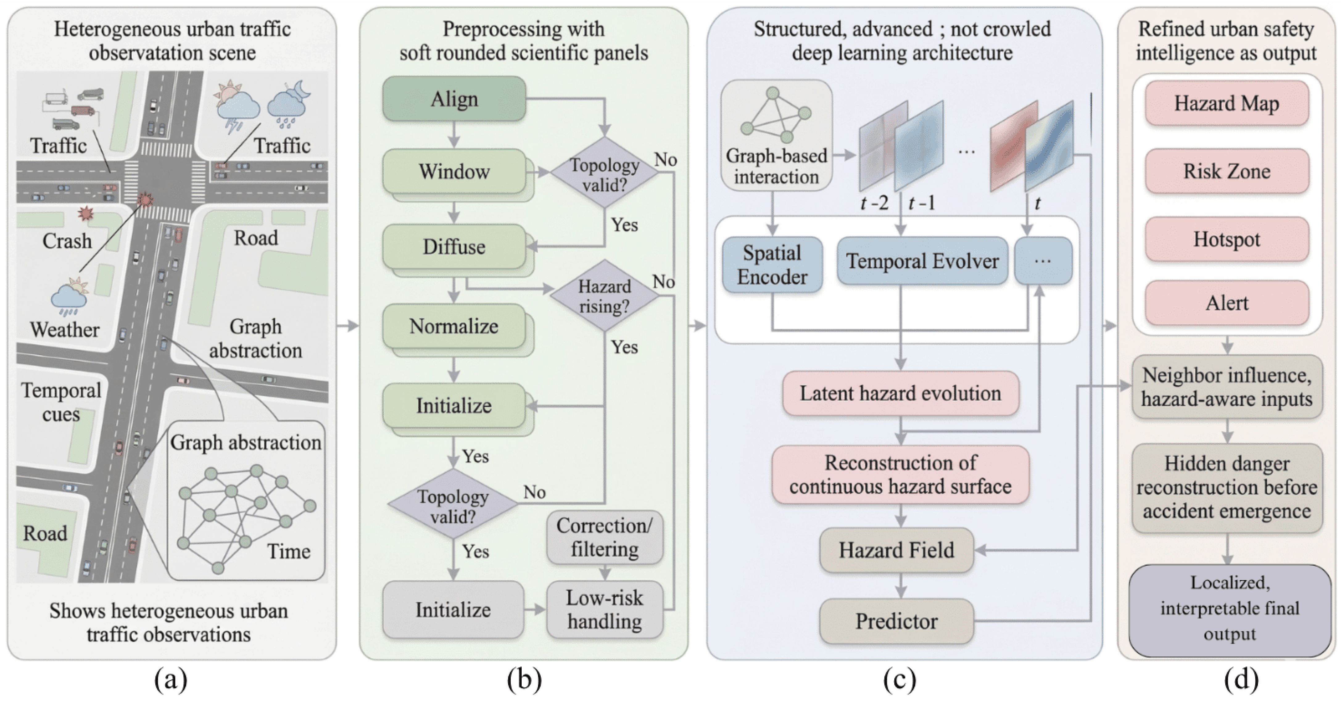
Although the proposed framework demonstrates strong promise, several directions remain open for future research. First, extending the framework to real-time streaming environments would strengthen its practical applicability for live traffic monitoring and early-warning systems. Second, incorporating richer urban context, such as signal timing, lane-level dynamics, multimodal mobility interaction, and detailed weather progression, may further improve the fidelity of hazard reconstruction. Third, evaluating the framework across additional cities, transportation networks, and external benchmark datasets would provide stronger evidence of generalizability and cross-domain robustness. Finally, future work could explore explainable hazard visualization, uncertainty-aware accident emergence modeling, and integration with traffic control or intervention systems to support decision-making in smart-city safety operations.   

Author Contributions

Conceptualization, N.L., M.A. and M.Q.A.-J.; methodology, N.L. and M.A.; software, M.A.; validation, N.L., M.A. and M.Q.A.-J.; formal analysis, N.L. and M.A.; investigation, N.L. and M.A.; resources, N.L. and M.Q.A.-J.; data curation, M.A.; writing—original draft preparation, N.L. and M.A.; writing—review and editing, N.L., M.A. and M.Q.A.-J.; visualization, M.A.; supervision, N.L. and M.Q.A.-J.; project administration, N.L.; funding acquisition, N.L. All authors have read and agreed to the published version of the manuscript.

Funding

This research was supported and funded by Al-Ahliyya University, Amman, Jordan.

Institutional Review Board Statement

Not applicable.

Informed Consent Statement

Not applicable.

Data Availability Statement

The datasets used in this study are publicly available from online sources. The XTraffic Incident Dataset (2022–2024) was obtained from Kaggle and consists of the files incidents_y2022.csv, incidents_y2023.csv, and incidents_y2024.csv. The Motor Vehicle Collisions–Crashes Dataset was also obtained from a publicly accessible online repository. These datasets were used to support the development, preprocessing, and evaluation of the proposed framework. Any derived data processing scripts, feature engineering procedures, and implementation details can be made available by the corresponding author upon reasonable request. https://www.kaggle.com/datasets/gpxlcj/xtraffic, https://doi.org/10.1016/j.aap.2024.107564 (accessed on 26 March 2026).

Conflicts of Interest

The authors declare no conflicts of interest.

References

  1. Adeniran, A.O.; Adeniran, A.A.; Ogieva, M.O.; Ogwuche, G. Adoption of Intelligent Transport Systems (ITS) in Urban Transportation Planning. Discov. Glob. Soc. 2026, 4, 13. [Google Scholar] [CrossRef]
  2. He, S.; Du, Z.; Wong, Y.D.; Ding, X.; Wu, P. Understanding the risk factors of driving dilemmas at urban tunnel exits adjoining diverging areas: A naturalistic study. Accid. Anal. Prev. 2026, 230, 108466. [Google Scholar] [CrossRef]
  3. Cansiz, O.F.; Can, M.F.; Unsalan, K. Identifying and Analysing Traffic Accident Hotspots–A Holistic Approach Combining Spatial and Data Mining Techniques. Promet—Traffic Transp. 2026, 38, 519–534. [Google Scholar] [CrossRef]
  4. Mansouryar, S. Smart Multimodal Corridor Control: Integrated AI and Model-Based Strategies for Urban and Extra-Urban Traffic Management. Ph.D. Thesis, Department of Civil, Constructional, and Environmental Engineering, Faculty of Civil and Industrial Engineering, Sapienza University of Rome, Rome, Italy, 2026. [Google Scholar]
  5. Tyagi, B.; Agrawal, A.; Jajaniya, H.; Bhardwaj, G. Smart Traffic Management and Accident Detection System: A Review. In DMPedia Lecture Notes in Computer Science & Engineering; Digital Manuscriptpedia: Greater Noida, India, 2026; pp. 335–345. [Google Scholar]
  6. Feng, J.; Qian, K.; Wang, Y. Traffic accident prediction model based on diffusion modeling and spatiotemporal dependency awareness. J. Supercomput. 2026, 82, 254. [Google Scholar] [CrossRef]
  7. Yang, Y.; Chen, X.; Wang, J.; Dong, Y.; Qie, K.; Yuan, Z. Enhancing vision-based traffic crash detection performance consistency across day-night scenes: A depth-aware and domain-adaptive network. Accid. Anal. Prev. 2026, 228, 108405. [Google Scholar] [CrossRef] [PubMed]
  8. Dzinyela, R.; Jafari, M.; Das, S.; Shimu, T.H.; Alnawmasi, N.; Lord, D. Unconstrained and partially constrained temporal modelling of pedestrian injury severities. Transp. A Transp. Sci. 2026, 22, 2388617. [Google Scholar] [CrossRef]
  9. Koramati, S.; Majumdar, B.B.; Sahu, P.K.; Das, S.; Ghosh, A.; Biswas, S. Segmentation of Risk Factors for Fatal Crashes at Urban Signalized Intersections: A Multi-Perspective Model Approach. Transp. Res. Rec. 2026, 03611981251407917. [Google Scholar] [CrossRef]
  10. Tan, Z.; Cui, L.; Xu, H.; Xu, J.; Feng, H.; Wang, P. A hybrid machine learning approach for predicting traffic accident collision severity. Int. J. Inj. Control Saf. Promot. 2026, 1–15. [Google Scholar] [CrossRef]
  11. Cui, P.; Yang, X.; Abdel-Aty, M.; Zhang, J.; Yan, X. Advancing urban traffic accident forecasting through sparse spatio-temporal dynamic learning. Accid. Anal. Prev. 2024, 200, 107564. [Google Scholar] [CrossRef]
  12. Liu, Z.; Chen, Y.; Xia, F.; Bian, J.; Zhu, B.; Shen, G.; Kong, X. TAP: Traffic accident profiling via multi-task spatio-temporal graph representation learning. ACM Trans. Knowl. Discov. From Data 2023, 17, 1–25. [Google Scholar] [CrossRef]
  13. Li, H.; Chen, L. Traffic accident risk prediction based on deep learning and spatiotemporal features of vehicle trajectories. PLoS ONE 2025, 20, e0320656. [Google Scholar] [CrossRef]
  14. Park, R.C.; Hong, E.J. Urban traffic accident risk prediction for knowledge-based mobile multimedia service. Personal. Ubiquitous Comput. 2022, 26, 417–427. [Google Scholar] [CrossRef]
  15. Macedo, M.R.; Maia, M.L.; Rabbani, E.R.K.; Neto, O.C.L.; Andrade, M. Traffic accident prediction model for rural highways in Pernambuco. Case Stud. Transp. Policy 2022, 10, 278–286. [Google Scholar] [CrossRef]
  16. Gou, X.; Li, Z.; Lan, T.; Lin, J.; Li, Z.; Zhao, B.; Zhang, C.; Wang, D.; Zhang, X. XTraffic: A Dataset Where Traffic Meets Incidents with Explainability and More. arXiv 2024, arXiv:2407.11477. [Google Scholar]
  17. Huang, B.; Hooi, B.; Shu, K. TAP: A Comprehensive Data Repository for Traffic Accident Prediction in Road Networks. In Proceedings of the 31st ACM International Conference on Advances in Geographic Information Systems; ACM: New York, NY, USA, 2023. [Google Scholar] [CrossRef]
  18. Wang, M.; Lee, W.-C.; Liu, N.; Fu, Q.; Wan, F.; Yu, G. A Data-Driven Deep Learning Framework for Prediction of Traffic Crashes at Road Intersections. Appl. Sci. 2025, 15, 752. [Google Scholar] [CrossRef]
  19. Yumak, A.; Tercan, S.H.; Colak, U.C.; Ozcanan, S. A Machine Learning Approach to Identify High-Risk Road Segments and Accident Severity Patterns Based on Categorical Data. Appl. Sci. 2025, 15, 12824. [Google Scholar] [CrossRef]
  20. Alnowaiser, K. A Computational Intelligence GNN–LSTM Framework for Spatiotemporal Prediction of Traffic Accident Severity in Smart Cities Using SHAP XAI. Int. J. Comput. Intell. Syst. 2025, 18, 271. [Google Scholar] [CrossRef]
  21. GPXLCJ. XTraffic Dataset. Kaggle. 2024. Available online: https://www.kaggle.com/datasets/gpxlcj/xtraffic (accessed on 4 April 2026).
  22. TUSH32. Motor Vehicle Collisions—Crashes. Kaggle. 2024. Available online: https://www.kaggle.com/datasets/tush32/motor-vehicle-collisions-crashes (accessed on 4 April 2026).
  23. Zeng, J. Machine learning for intelligent transportation systems. In Proceedings of the International Conference on Frontiers of Traffic and Transportation Engineering (FTTE 2025), Guilin, China, 31 October–2 November 2026; Volume 14060, pp. 427–432. [Google Scholar]
  24. Carvalho, C.; Ribeiro, P.J.G.; José, R.J.P. Systematic identification and analysis of map-matching anomalies in road network models for urban cycling. Environ. Plan. B Urban Anal. City Sci. 2026, 23998083251415038. [Google Scholar] [CrossRef]
  25. Mashhadi Moghaddam, S.N.; Cao, H. Exploring spatial patterns of immigrant settlement in Toronto using spatial Gaussian-Bernoulli DBN and GraphSAGE. Environ. Plan. B Urban Anal. City Sci. 2026, 23998083261428174. [Google Scholar] [CrossRef]
  26. Gao, Z.; Peng, S.; Song, Z.; Sun, Y.; Xu, W.; Lai, L.; Chen, S. Small-World Topology and Graph Attention Reinforcement Learning for dynamic traffic optimization. Eng. Appl. Artif. Intell. 2026, 167, 113919. [Google Scholar] [CrossRef]
  27. Li, Y.; Xu, Y.; He, X.; Zhu, D.; Zhang, Y.; Zhang, J. A security-oriented four-factor spatio-temporal framework for assessing and mitigating traffic congestion risks. Sci. Rep. 2026, 16, 9548. [Google Scholar] [CrossRef]
  28. Ni, Y.-C.; Kouvelas, A.; Makridis, M.A. Simulating link-level interrupted flow traffic dynamics and the comparison between different models for urban road networks. Simul. Model. Pract. Theory 2026, 103252. [Google Scholar] [CrossRef]
  29. Liu, J.; Shen, K.; Liu, X. Nonlinear Effects of Multilevel Urban Environments on Traffic Crash Risk: A Multiscale Analysis with Explainable Machine Learning. Trans. GIS 2026, 30, e70200. [Google Scholar] [CrossRef]
  30. Hao, S.; Zhao, X.; Wang, J.; Gong, X. Efficient Directed Hypergraph Network for Unsupervised Traffic Anomaly Detection: A Survey. IEEE Intell. Transp. Syst. Mag. 2026, 18, 86–98. [Google Scholar] [CrossRef]
  31. Yuan, W.; Wu, S.; Shen, C. A traffic flow prediction model incorporating hybrid spatio-temporal features and dynamic diffusion graph convolution. Clust. Comput. 2026, 29, 169. [Google Scholar] [CrossRef]
  32. Abibulaiev, A.; Pukach, P.; Vovk, M. Context-Aware ML/NLP Pipeline for Real-Time Anomaly Detection and Risk Assessment in Cloud API Traffic. Mach. Learn. Knowl. Extr. 2026, 8, 25. [Google Scholar] [CrossRef]
  33. Wang, Z.; Zhang, L.; Guo, J.; Huang, Y.; Ping, L.; Zheng, W.; Zhangzhong, L. LGCA-Net: A time-series anomaly detection method for multiple types of agricultural sensors. Inf. Process. Agric. 2026, in press. [Google Scholar] [CrossRef]
  34. Abubakar, M.; Usman, U. Spatial Analysis of Road Traffic Accident Hotspots in Jega, Nigeria: A Comparative Study of Kernel Density Estimation and Geographically Weighted Regression. Preprints 2026. [Google Scholar] [CrossRef]
  35. Guo, Y.; Luo, Y.; Cui, P.; Liu, G.; Liu, W.; Liu, P. Crash hotspot identification using large-scale trajectory data: Insights from surrogate safety measures. J. Transp. Saf. Secur. 2026, 1–29. [Google Scholar] [CrossRef]
  36. Zhang, Y.; Guo, X.; Zhang, Y. A multibranch risk assessment model for multi-lane highway work zones based on risk fields and graph attention network. J. Transp. Saf. Secur. 2026, 1–36. [Google Scholar] [CrossRef]
  37. Qin, H.; Wang, D. Estimating Instantaneous Traffic Flow from Event-Time Detectors: An Adaptive Kernel-Intensity Observer for Emerging Transport Systems. SSRN 2026. [Google Scholar] [CrossRef]
  38. Morozov, V.; Petrov, A.I.; Shepelev, V.; Balfaqih, M. Ideology of urban road transport chaos and accident risk management for sustainable transport systems. Sustainability 2024, 16, 2596. [Google Scholar] [CrossRef]
  39. Al-Jamal, M.Q.; Alsarhan, A.; AlJamal, M.; Aljamal, Q.; Khassawneh, B.S.; Salhi, A.; Hayat, H. Integrating Generative Design and Artificial Intelligence for Optimized Energy-Efficient Composite Facades in Next-Generation Smart Buildings. Sustainability 2026, 18, 2379. [Google Scholar] [CrossRef]
Figure 1. Proposed Methodology, (a) Urban observation layer, (b) Intelligent preprocessing layer, (c) Core learning architecture, (d) Output layer.
Urbansci 10 00300 g001
Figure 2. Topology-Aware Spatio-Temporal Hazard Field Preconditioning Pipeline.
Urbansci 10 00300 g002
Figure 3. Transformation of urban traffic risk representation before and after hazard-aware preprocessing. The colored dots in the left panel represent sparse observed traffic-risk/event points before preprocessing, with different colors indicating different initial normalized risk intensities. The right panel shows the corresponding continuous hazard field after preprocessing, where the discrete observations are redistributed into a smooth spatial hazard representation.
Urbansci 10 00300 g003
Figure 4. Transformation of Sparse Incident Evidence into a Continuous Urban Hazard Surface in the XTraffic Incident Dataset.
Urbansci 10 00300 g004
Figure 5. Spatial Risk Topology of the XTraffic Incident Dataset Before and After Continuous Hazard-Field Construction.
Urbansci 10 00300 g005
Figure 6. Spatio-Temporal Hazard Structure of the XTraffic Incident Dataset Before and After Hazard-Aware Preprocessing.
Urbansci 10 00300 g006
Figure 7. Transformation of Sparse Incident Evidence into a Continuous Urban Hazard Surface in the Motor Vehicle Collisions Crashes Dataset.
Urbansci 10 00300 g007
Figure 8. Spatial Risk Topology of the Motor Vehicle Collisions Crashes Dataset Before and After Continuous Hazard-Field Construction.
Urbansci 10 00300 g008
Figure 9. Spatio-Temporal Hazard Structure of the Motor Vehicle Collisions Crashes Dataset Before and After Hazard-Aware Preprocessing.
Urbansci 10 00300 g009
Figure 10. Temporal Evolution of the Urban Hazard Field and Accident Emergence Mapping.
Urbansci 10 00300 g010
Figure 11. Proposed Deep Learning Architecture for Continuous Hazard Field Learning and Localized Accident Emergence Prediction.
Urbansci 10 00300 g011
Figure 12. Multi-Perspective Performance Evaluation of Baseline Experiment E1 across Training and Testing Stages.
Urbansci 10 00300 g012
Figure 13. Multi-Perspective Performance Evaluation of Baseline Experiment E1 across Training and Testing Stages.
Urbansci 10 00300 g013
Figure 14. Multi-Perspective Performance Evaluation of Baseline Experiment E1 across Training and Testing Stages.
Urbansci 10 00300 g014
Figure 15. Multi-Perspective Performance Evaluation of Baseline Experiment E1 across Training and Testing Stages.
Urbansci 10 00300 g015
Figure 16. Multi-Perspective Performance Evaluation of Baseline Experiment E1 across Training and Testing Stages.
Urbansci 10 00300 g016
Figure 17. Multi-Perspective Comparative Analysis of Block E4 across Metric, Ranking, Confusion, and Training-Stability Views.
Urbansci 10 00300 g017
Figure 18. Spatial Hazard Topology Learned by Experiment E6 on Dataset 1.
Urbansci 10 00300 g018
Figure 19. Incremental Component Contribution Analysis of Experiment E7 on Dataset 1.
Urbansci 10 00300 g019
Figure 20. Spatio-Temporal Hazard Intensity Evolution Learned by Experiment E8 on Dataset 1.
Urbansci 10 00300 g020
Figure 21. Ablation Heatmap of Experiment E8 across Core Architectural Components on Dataset 1.
Urbansci 10 00300 g021
Figure 22. Discriminative Ranking Performance of Block E9 through ROC and Precision-Recall Analysis on Dataset 1.
Urbansci 10 00300 g022
Figure 23. Temporal Hazard Dynamics Alignment of Block E9 on Dataset 1.
Urbansci 10 00300 g023
Figure 24. Final Classification Reliability and Confidence Calibration of Block E10 on Dataset 1.
Urbansci 10 00300 g024
Table 1. Features and its dicription of Dataset 1 (XTraffic Incident Dataset, 2022–2024).
FeatureDescriptionData TypeSample ValueAnalytical Relevance
incident_idUnique identifier assigned to each incident record.Identifier/mixed numeric-text20,660,604Used for record tracking, integrity checking, and duplicate handling.
durationDuration of the incident, typically reflecting how long the event remained active or reported.Numerical (continuous)1065.0Indicates persistence and operational severity of an event; useful for distinguishing transient incidents from prolonged disruptions.
Abs PMAbsolute postmile or linear roadway position associated with the incident.Numerical (continuous)385.1Supports fine-grained linear localization along freeway segments and enhances road-aligned spatial modeling.
FwyFreeway number or corridor identifier where the incident occurred.Numerical/route code101.0Encodes the primary transportation corridor and can reveal route-specific risk concentration.
AREATraffic management area or geographic reporting region.Categorical (text)San JoseCaptures regional traffic context and supports spatial stratification across administrative or operational areas.
DESCRIPTIONTextual description of the incident type or operational event.Text/categorical descriptor1183-Trfc Collision-Unkn InjProvides semantic interpretation of the incident and supports event-type grouping or natural-language-informed categorization.
LOCATIONHuman-readable roadway location description.TextUs101 N/Alum Rock Ave OfrProvides locational specificity at ramps, junctions, and corridor subsegments; useful for intersection and interchange analysis.
dtDate and time stamp of the incident.Datetime/temporal string1 January 2022 00:00:00Enables temporal ordering, time-window construction, rush-hour analysis, and seasonal or weekly pattern extraction.
LatitudeGeographic latitude coordinate of the event.Numerical (continuous)37.346961Supports geographic mapping, network alignment, and spatial hazard surface construction.
LongitudeGeographic longitude coordinate of the event.Numerical/mixed-format field−121.858883Complements latitude for precise spatial localization and roadway graph projection.
Freeway directionTravel direction associated with the event.Categorical (text)NEncodes directional traffic flow, which is essential for corridor-level hazard propagation and directional congestion interpretation.
TypeCondensed incident category label.Categorical (text)UnknInj, Hazard, NoInjUseful as an operational event grouping variable and as a semantic indicator of incident severity or roadway condition class.
Table 2. Feature-level documentation of Dataset 2 (Motor Vehicle Collisions—Crashes Dataset).
FeatureDescriptionData TypeSample ValueAnalytical Relevance
CRASH DATECalendar date on which the collision occurred.Date/text-formatted temporal field9 November 2021Supports daily, monthly, and long-term temporal pattern analysis.
CRASH TIMEReported time of collision occurrence.Time/text-formatted temporal field2:39Useful for identifying time-of-day risk peaks and rush-hour or nighttime crash patterns.
BOROUGHBorough in which the collision was recorded.Categorical (text)BROOKLYNProvides broad urban spatial context and supports borough-level safety stratification.
ZIP CODEPostal zone associated with the crash location.Numerical/mixed geographic code11,354Adds finer local geographic granularity for zone-based accident analysis.
LATITUDELatitude coordinate of the crash site.Numerical (continuous)40.768875Enables precise spatial mapping and geographic hotspot identification.
LONGITUDELongitude coordinate of the crash site.Numerical (continuous)−73.830970Complements latitude for detailed spatial positioning and map-based modeling.
LOCATIONCombined point-location representation.Text/coordinate descriptor(40.768875, −73.83097)Supports location verification and integrated spatial parsing.
ON STREET NAMEPrimary roadway name where the collision occurred.Categorical (text)WHITESTONE EXPRESSWAYProvides direct roadway identity for segment-level or corridor-level crash studies.
CROSS STREET NAMECross street associated with the collision location.Categorical (text)20 AVENUEImportant for intersection-focused analysis and conflict-zone identification.
OFF STREET NAMEOff-street location descriptor when the crash is not directly tied to a standard street intersection.Categorical (text)QUEENSBORO BRIDGE UPPERCaptures nonstandard location contexts such as bridges, service roads, or facilities.
NUMBER OF PERSONS INJUREDTotal number of injured persons in the crash.Numerical (integer)2Direct indicator of crash severity and human impact.
NUMBER OF PERSONS KILLEDTotal number of fatalities in the crash.Numerical (integer)0High-severity outcome variable for fatal crash assessment.
NUMBER OF PEDESTRIANS INJUREDNumber of pedestrians injured in the crash.Numerical (integer)0Supports vulnerable road-user safety analysis.
NUMBER OF PEDESTRIANS KILLEDNumber of pedestrian fatalities.Numerical (integer)0Captures extreme vulnerable-user crash outcomes.
NUMBER OF CYCLIST INJUREDNumber of cyclists injured.Numerical (integer)0Relevant for multimodal urban mobility safety assessment.
NUMBER OF CYCLIST KILLEDNumber of cyclist fatalities.Numerical (integer)0Important for severe cyclist safety analysis.
NUMBER OF MOTORIST INJUREDNumber of motorists injured.Numerical (integer)2Differentiates motorist-specific injury burden from total injuries.
NUMBER OF MOTORIST KILLEDNumber of motorist fatalities.Numerical (integer)0Supports fatality-oriented driver and passenger risk analysis.
CONTRIBUTING FACTOR VEHICLE 1Primary reported contributing factor for the first vehicle.Categorical (text)Aggressive Driving/Road RageHighly informative for behavioral and causal interpretation of crash genesis.
CONTRIBUTING FACTOR VEHICLE 2Secondary contributing factor associated with the second vehicle.Categorical (text)UnspecifiedSupports multi-vehicle cause interaction analysis.
CONTRIBUTING FACTOR VEHICLE 3Additional contributing factor for a third involved vehicle, when available.Categorical/sparse text-Extends behavioral attribution in multi-vehicle crashes.
CONTRIBUTING FACTOR VEHICLE 4Additional contributing factor for a fourth involved vehicle, when available.Categorical/sparse text-Useful for complex crash events with multiple participants.
CONTRIBUTING FACTOR VEHICLE 5Additional contributing factor for a fifth involved vehicle, when available.Categorical/sparse text-Captures extended multi-vehicle crash complexity.
COLLISION_IDUnique identifier of the collision record.Identifier (integer)4,455,765Supports indexing, linking, and record-level integrity.
VEHICLE TYPE CODE 1Vehicle class of the first involved vehicle.Categorical (text)SedanSupports analysis of vehicle composition in crash outcomes.
VEHICLE TYPE CODE 2Vehicle class of the second involved vehicle.Categorical (text)SedanUseful for pairwise vehicle-interaction studies.
VEHICLE TYPE CODE 3Vehicle class of a third vehicle when present.Categorical/sparse text-Adds contextual detail in multi-vehicle events.
VEHICLE TYPE CODE 4Vehicle class of a fourth vehicle when present.Categorical/sparse text-Supports extended crash composition analysis.
VEHICLE TYPE CODE 5Vehicle class of a fifth vehicle when present.Categorical/sparse text-Captures rare but structurally complex multi-vehicle collisions.
Table 3. Prediction targets, label construction, excluded variables, and leakage-control strategy.
DatasetPrediction TargetLabel ConstructionVariables Excluded from InputsLeakage-Control Check
Dataset 1: XTraffic Incident DatasetOperational incident-risk category predictionIncident categories were mapped into the final experimental risk classes using y i ( 1 ) = g 1 ( Type i , DESCRIPTION i ) .DESCRIPTION, Type, and any textual or categorical field directly encoding or duplicating the incident class.Target-like fields were removed after label construction; only non-label spatial, temporal, roadway, directional, contextual, and engineered hazard features were retained.
Dataset 2: Motor Vehicle Collisions–CrashesCrash-severity prediction: No Injury, Minor Injury, Multi-Injury, and Fatal/SevereSeverity labels were generated from injury and fatality counts using y i ( 2 ) = g 2 ( I i , F i ) , then the count variables were removed.All injury and fatality count variables; post-outcome variables; target-proxy fields; contributing-factor and vehicle-type fields when unavailable before the prediction point.Label-generating variables were removed before training; train–test split was performed before preprocessing; final feature audit was conducted to prevent target leakage.
Table 4. Temporal hazard window embedding strategy.
ComponentInputOperationOutput
Raw Temporal RecordsTime-stamped traffic and contextual observationsCollect sequential measurements for each road segment or intersectionOrdered temporal sequence
Overlapping WindowingOrdered temporal sequencePartition data into partially overlapping windows of length W with stride Δ Local hazard evolution intervals
Temporal Context PreservationWindowed observationsRetain recent traffic, environmental, and conflict history within each intervalPre-crash temporal dependency patterns
Hazard Trajectory EncodingConsecutive overlapping windowsTrack gradual instability buildup across neighboring time intervalsContinuous hazard progression cues
Learning-Ready RepresentationEmbedded temporal windowsOrganize each network unit as a spatio-temporal sequence for downstream modelingHazard-aware temporal feature tensor
Table 5. Advanced formulation of continuous hazard surface initialization.
Processing LayerInput RepresentationCore OperationOutput Representation
Event Acquisition LayerAccident points, surrogate conflict indicators, event timestamps, and event severity weightsCollect sparse safety evidence from crash records and high-risk traffic interactions; assign each event a spatial coordinate, temporal index, and hazard contribution magnitudeDiscrete event set S = { ( s k , t k , y k ) } k = 1 M
Spatial Influence Diffusion LayerDiscrete event set with mapped network locationsSpread each event over nearby road segments and intersections through distance-decay kernels so that hazard influence extends beyond the exact crash coordinate into adjacent infrastructure unitsLocalized spatial hazard support field
Temporal Continuity Embedding LayerSpatially diffused event signals with timestampsPropagate hazard influence across neighboring temporal intervals to preserve pre-event buildup and short-term post-event continuity, thereby avoiding purely instantaneous event encodingSpatio-temporal event influence volume
Multi-Event Hazard Aggregation LayerOverlapping spatial and temporal hazard contributions from all eventsSuperimpose weighted kernel responses from all incidents to construct a unified initial hazard intensity surface reflecting cumulative risk concentration and interaction overlapContinuous raw hazard field H 0 ( s , t )
Topology-Constrained Projection LayerContinuous raw hazard field and road-network graph structureProject aggregated hazard intensity onto valid transportation units while respecting network geometry, segment adjacency, and intersection connectivityNetwork-consistent hazard surface
Normalization and Learning Interface LayerProjected hazard surface over network units and timeRescale hazard magnitudes into a stable bounded range and organize them into model-ready tensors or graph-aligned feature maps for downstream continuous hazard learningLearning-ready continuous hazard representation
Table 6. Major components in the proposed deep learning architecture.
ModuleInputOperationOutput
Hazard-Aware Input RepresentationPreprocessed multi-source urban traffic observations, topology-aligned network units, temporal windows, and initialized hazard informationOrganize traffic flow, speed variance, congestion density, road geometry, weather disturbance, temporal context, and initial hazard cues into graph-aligned feature matrices or spatio-temporal tensors over road segments and intersectionsStructured hazard-aware spatio-temporal input representation
Spatial Hazard Encoding ModuleHazard-aware spatio-temporal input representation and transportation graph connectivityLearn topology-aware interactions among connected road segments and intersections through graph-based spatial encoding, message passing, and neighboring hazard aggregation to capture corridor-level instability and network-driven risk transferLatent spatial hazard embedding
Temporal Hazard Evolution ModuleLatent spatial hazard embedding across successive time intervalsModel hazard persistence, gradual buildup, escalation, and temporal dependency using sequential learning over time-ordered latent hazard statesTemporally evolved hazard representation
Continuous Hazard Reconstruction LayerTemporally evolved hazard representation and graph-structured urban network contextRefine internal deep features into a continuous latent hazard field that preserves spatial continuity, temporal coherence, and smooth risk variation across road segments and intersectionsReconstructed continuous hidden-danger field
Accident Emergence Prediction HeadReconstructed continuous hidden-danger field, hazard escalation cues, and neighborhood hazard contextMap latent hazard intensity, temporal escalation, and surrounding network reinforcement into localized accident emergence probability for each spatial unit and time intervalFine-grained accident emergence probability field
End-to-End Training StrategyAll architectural modules, labeled accident-emergence targets, and hazard-consistency objectivesJointly optimize spatial encoding, temporal hazard learning, hazard reconstruction, and prediction through unified end-to-end training with rare-event handling, regularization, and adaptive optimizationTrained continuous hazard field intelligence model
Table 7. Configuration of experiments for continuous hazard field learning and accident emergence prediction.
Exp.ObjectiveSpatial EncoderTemporal ModuleHazard ReconstructionPrediction Head W ,   Δ h α , β Training Setting
E1Baseline tabular accident prediction without hazard-field modelingNoneNoneNoneMLP only 1 ,   1 64-Adam, 10 3 , batch 64, 60 epochs
E2Add topology-aware spatial encoding onlyGCN-based spatial encoderNoneNoneSigmoid emergence head 1 ,   1 64 α = 0.70 , β = 0 Adam, 10 3 , batch 64, 70 epochs
E3Add temporal hazard evolution without spatial couplingNoneGRUNoneSigmoid emergence head 6 ,   2 96 α = 1.00 , β = 0.60 Adam, 8 × 10 4 , batch 64, 80 epochs
E4Joint spatial-temporal encoding without reconstruction layerGCN-based spatial encoderGRUNoneSigmoid emergence head 6 ,   2 128 α = 0.70 , β = 0.60 Adam, 8 × 10 4 , batch 64, 90 epochs
E5Add continuous hazard reconstruction layerGCN-based spatial encoderGRULinear + ReLU hazard field layerSigmoid emergence head 6 ,   2 128 α = 0.70 , β = 0.65 Adam, 5 × 10 4 , batch 64, 100 epochs
E6Full model with risk-diffusion feature liftingGCN + lifted topology diffusionGRUHazard field reconstructionSigmoid emergence head 8 ,   2 128 α = 0.65 , β = 0.70 Adam, 5 × 10 4 , batch 64, 100 epochs
E7Full model with hazard-escalation cue  Δ H b ( t ) GCN + lifted topology diffusionGRUHazard field reconstructionHazard + escalation prediction head 8 ,   2 160 α = 0.65 , β = 0.75 Adam, 3 × 10 4 , batch 64, 110 epochs
E8Full model with neighborhood hazard context W H b ( t ) GCN + lifted topology diffusionGRUHazard field reconstructionHazard + escalation + neighborhood head 8 ,   2 160 α = 0.60 , β = 0.75 Adam, 3 × 10 4 , batch 64, 110 epochs
E9Stronger temporal modeling for long hazard buildupGCN + lifted topology diffusionBiGRUHazard field reconstructionFull emergence mapping head 10 ,   3 192 α = 0.60 , β = 0.80 Adam, 2 × 10 4 , batch 32, 120 epochs
E10Final proposed CHFI frameworkGCN + topology-aware diffusionBiGRU + temporal memory updateContinuous hazard reconstruction layerFull accident-emergence head using H b ( t ) , Δ H b ( t ) , and  W H b ( t ) 10 ,   3 256 α = 0.60 , β = 0.80 Adam, 2 × 10 4 , batch 32, 120 epochs, early stopping
Table 8. Reorganized reporting structure of the Results and Discussion section.
Results BlockMain ContentPurpose
Evaluation protocolDatasets, validation settings, metrics, and reporting logic.Separates the experimental setup from performance interpretation.
Training resultsTraining-stage accuracy, precision, recall, F1-score, AUC, and convergence behavior.Examines learning stability before evaluating unseen-data performance.
Testing resultsHeld-out predictive performance on Dataset 1 and Dataset 2.Assesses model generalization without blending it with training-stage findings.
Comparative analysisComparison between the proposed CHFI model, baseline models, and reduced configurations.Highlights relative performance trends instead of repeating all table values.
Ablation analysisComponent-level evaluation of spatial encoding, temporal modeling, hazard reconstruction, and diffusion-based feature lifting.Identifies which framework components contribute most to the final performance.
Visual diagnosticsConfusion matrices, ROC curves, precision–recall curves, and hazard-field visualizations.Supports interpretability and explains model behavior beyond scalar metrics.
Computational costInference time, memory use, complexity, and practical feasibility indicators.Connects predictive performance with deployment practicality.
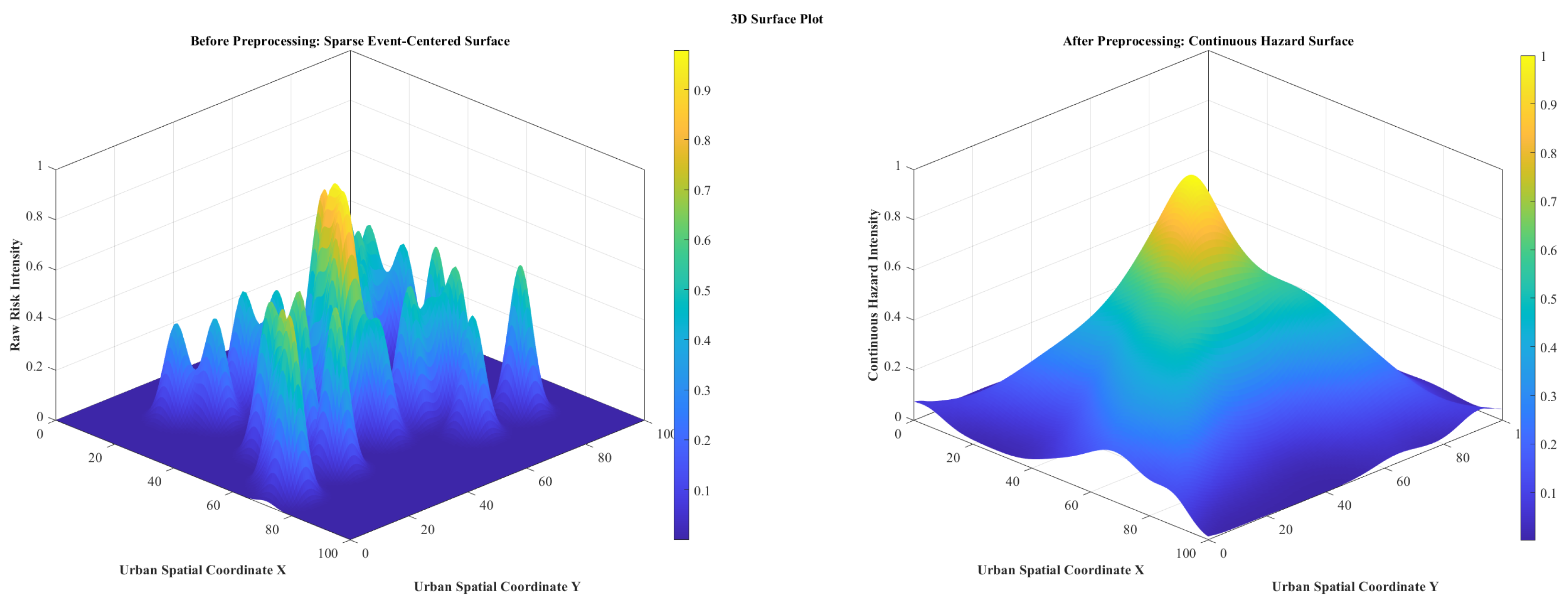
Table 9. Training Stage experimental results and architectural configurations across E1–E10 on the two traffic safety datasets.
Exp.Spatial EncoderTemporal ModuleHazard Recon.Prediction HeadTraining Setting W ,   Δ h α ,   β Acc. (%)Prec. (%)Rec. (%)F1 (%)AUC
Dataset 1: XTraffic Incident Dataset (2022-2024)
E1NoneNoneNoneMLP onlyAdam, 10 3 , batch 64, 60 ep. 1 ,   1 64-91.8491.1290.7690.940.944
E2GCN-based encoderNoneNoneSigmoid emergence headAdam, 10 3 , batch 64, 70 ep. 1 ,   1 64 α = 0.70 , β = 0 93.2792.8892.4192.640.956
E3NoneGRUNoneSigmoid emergence headAdam, 8 × 10 4 , batch 64, 80 ep. 6 ,   2 96 α = 1.00 , β = 0.60 93.9693.5193.0793.290.962
E4GCN-based encoderGRUNoneSigmoid emergence headAdam, 8 × 10 4 , batch 64, 90 ep. 6 ,   2 128 α = 0.70 , β = 0.60 95.1894.8694.5294.690.972
E5GCN-based encoderGRULinear + ReLU layerSigmoid emergence headAdam, 5 × 10 4 , batch 64, 100 ep. 6 ,   2 128 α = 0.70 , β = 0.65 96.0495.7395.3695.540.978
E6GCN + lifted diffusionGRUHazard field recon.Sigmoid emergence headAdam, 5 × 10 4 , batch 64, 100 ep. 8 ,   2 128 α = 0.65 , β = 0.70 96.7196.3896.0596.210.983
E7GCN + lifted diffusionGRUHazard field recon.Hazard + escalation headAdam, 3 × 10 4 , batch 64, 110 ep. 8 ,   2 160 α = 0.65 , β = 0.75 97.4897.1696.8997.020.988
E8GCN + lifted diffusionGRUHazard field recon.Hazard + escalation + neighborhood headAdam, 3 × 10 4 , batch 64, 110 ep. 8 ,   2 160 α = 0.60 , β = 0.75 98.0397.7897.4297.600.991
E9GCN + lifted diffusionBiGRUHazard field recon.Full emergence mapping headAdam, 2 × 10 4 , batch 32, 120 ep. 10 ,   3 192 α = 0.60 , β = 0.80 98.5698.2998.0598.170.995
E10GCN + topology-aware diffusionBiGRU + memory updateContinuous recon. layerFull accident-emergence head using H b ( t ) , Δ H b ( t ) , W H b ( t ) Adam, 2 × 10 4 , batch 32, 120 ep., early stop 10 ,   3 256 α = 0.60 , β = 0.80 99.1298.9498.7698.850.998
Dataset 2: Motor Vehicle Collisions-Crashes Dataset
E1NoneNoneNoneMLP onlyAdam, 10 3 , batch 64, 60 ep. 1 ,   1 64-90.9690.2189.8490.020.936
E2GCN-based encoderNoneNoneSigmoid emergence headAdam, 10 3 , batch 64, 70 ep. 1 ,   1 64 α = 0.70 , β = 0 92.3491.9891.4291.700.949
E3NoneGRUNoneSigmoid emergence headAdam, 8 × 10 4 , batch 64, 80 ep. 6 ,   2 96 α = 1.00 , β = 0.60 93.0892.6692.1492.400.956
E4GCN-based encoderGRUNoneSigmoid emergence headAdam, 8 × 10 4 , batch 64, 90 ep. 6 ,   2 128 α = 0.70 , β = 0.60 94.4194.0293.6893.850.968
E5GCN-based encoderGRULinear + ReLU layerSigmoid emergence headAdam, 5 × 10 4 , batch 64, 100 ep. 6 ,   2 128 α = 0.70 , β = 0.65 95.2794.9594.6394.790.975
E6GCN + lifted diffusionGRUHazard field recon.Sigmoid emergence headAdam, 5 × 10 4 , batch 64, 100 ep. 8 ,   2 128 α = 0.65 , β = 0.70 95.9695.6195.2495.420.981
E7GCN + lifted diffusionGRUHazard field recon.Hazard + escalation headAdam, 3 × 10 4 , batch 64, 110 ep. 8 ,   2 160 α = 0.65 , β = 0.75 96.7496.3996.0896.230.987
E8GCN + lifted diffusionGRUHazard field recon.Hazard + escalation + neighborhood headAdam, 3 × 10 4 , batch 64, 110 ep. 8 ,   2 160 α = 0.60 , β = 0.75 97.3197.0496.7196.870.990
E9GCN + lifted diffusionBiGRUHazard field recon.Full emergence mapping headAdam, 2 × 10 4 , batch 32, 120 ep. 10 ,   3 192 α = 0.60 , β = 0.80 97.8997.6397.3897.500.994
E10GCN + topology-aware diffusionBiGRU + memory updateContinuous recon. layerFull accident-emergence head using H b ( t ) , Δ H b ( t ) , W H b ( t ) Adam, 2 × 10 4 , batch 32, 120 ep., early stop 10 ,   3 256 α = 0.60 , β = 0.80 98.6398.4198.1698.280.997
Table 10. Test-stage results and architectural configurations across E1–E10 on the two traffic safety datasets.
Exp.Spatial EncoderTemporal ModuleHazard Recon.Prediction HeadTraining Setting W ,   Δ h α ,   β Test Acc. (%)Test Prec. (%)Test Rec. (%)Test F1 (%)AUCTest Loss
Dataset 1: XTraffic Incident Dataset (2022–2024)
E1NoneNoneNoneMLP onlyAdam, 10 3 , batch 64, 60 ep. 1 ,   1 64-90.9190.2489.8890.060.9380.312
E2GCN-based encoderNoneNoneSigmoid emergence headAdam, 10 3 , batch 64, 70 ep. 1 ,   1 64 α = 0.70 , β = 0 92.3691.9491.5391.730.9510.278
E3NoneGRUNoneSigmoid emergence headAdam, 8 × 10 4 , batch 64, 80 ep. 6 ,   2 96 α = 1.00 , β = 0.60 93.1192.6892.2192.440.9580.259
E4GCN-based encoderGRUNoneSigmoid emergence headAdam, 8 × 10 4 , batch 64, 90 ep. 6 ,   2 128 α = 0.70 , β = 0.60 94.5894.1993.8294.000.9700.224
E5GCN-based encoderGRULinear + ReLU layerSigmoid emergence headAdam, 5 × 10 4 , batch 64, 100 ep. 6 ,   2 128 α = 0.70 , β = 0.65 95.4395.0994.7694.920.9770.201
E6GCN + lifted diffusionGRUHazard field recon.Sigmoid emergence headAdam, 5 × 10 4 , batch 64, 100 ep. 8 ,   2 128 α = 0.65 , β = 0.70 96.1895.8495.5195.670.9830.181
E7GCN + lifted diffusionGRUHazard field recon.Hazard + escalation headAdam, 3 × 10 4 , batch 64, 110 ep. 8 ,   2 160 α = 0.65 , β = 0.75 97.0196.7396.4196.570.9880.156
E8GCN + lifted diffusionGRUHazard field recon.Hazard + escalation + neighborhood headAdam, 3 × 10 4 , batch 64, 110 ep. 8 ,   2 160 α = 0.60 , β = 0.75 97.6297.3497.0297.180.9920.139
E9GCN + lifted diffusionBiGRUHazard field recon.Full emergence mapping headAdam, 2 × 10 4 , batch 32, 120 ep. 10 ,   3 192 α = 0.60 , β = 0.80 98.2197.9897.7197.840.9960.117
E10GCN + topology-aware diffusionBiGRU + memory updateContinuous recon. layerFull accident-emergence head using H b ( t ) , Δ H b ( t ) , W H b ( t ) Adam, 2 × 10 4 , batch 32, 120 ep., early stop 10 ,   3 256 α = 0.60 , β = 0.80 98.8498.6298.3798.490.9980.089
Dataset 2: Motor Vehicle Collisions-Crashes Dataset
E1NoneNoneNoneMLP onlyAdam, 10 3 , batch 64, 60 ep. 1 ,   1 64-90.0289.3188.9789.140.9310.328
E2GCN-based encoderNoneNoneSigmoid emergence headAdam, 10 3 , batch 64, 70 ep. 1 ,   1 64 α = 0.70 , β = 0 91.4791.0890.6290.850.9440.291
E3NoneGRUNoneSigmoid emergence headAdam, 8 × 10 4 , batch 64, 80 ep. 6 ,   2 96 α = 1.00 , β = 0.60 92.2891.8691.3991.620.9520.271
E4GCN-based encoderGRUNoneSigmoid emergence headAdam, 8 × 10 4 , batch 64, 90 ep. 6 ,   2 128 α = 0.70 , β = 0.60 93.7493.3692.9893.170.9650.236
E5GCN-based encoderGRULinear + ReLU layerSigmoid emergence headAdam, 5 × 10 4 , batch 64, 100 ep. 6 ,   2 128 α = 0.70 , β = 0.65 94.6394.2793.9694.110.9730.212
E6GCN + lifted diffusionGRUHazard field recon.Sigmoid emergence headAdam, 5 × 10 4 , batch 64, 100 ep. 8 ,   2 128 α = 0.65 , β = 0.70 95.3294.9894.6394.800.9800.193
E7GCN + lifted diffusionGRUHazard field recon.Hazard + escalation headAdam, 3 × 10 4 , batch 64, 110 ep. 8 ,   2 160 α = 0.65 , β = 0.75 96.0995.7895.4695.620.9860.169
E8GCN + lifted diffusionGRUHazard field recon.Hazard + escalation + neighborhood headAdam, 3 × 10 4 , batch 64, 110 ep. 8 ,   2 160 α = 0.60 , β = 0.75 96.7496.4596.1196.280.9900.149
E9GCN + lifted diffusionBiGRUHazard field recon.Full emergence mapping headAdam, 2 × 10 4 , batch 32, 120 ep. 10 ,   3 192 α = 0.60 , β = 0.80 97.3697.1296.8496.980.9940.126
E10GCN + topology-aware diffusionBiGRU + memory updateContinuous recon. layerFull accident-emergence head using H b ( t ) , Δ H b ( t ) , W H b ( t ) Adam, 2 × 10 4 , batch 32, 120 ep., early stop 10 ,   3 256 α = 0.60 , β = 0.80 98.0797.8697.5997.720.9970.101
Table 11. Ablation study of major CHFI components across the two datasets.
ConfigurationSpatial Enc.Temporal Evol.Hazard Recon.Diffusion LiftEscalation CueNbr. ContextF1 (D1) Δ F1 (D1)F1 (D2) Δ F1 (D2)
Baseline MLP------90.94-90.02-
Spatial-only hazard modeling-----92.64+1.7091.70+1.68
Temporal-only hazard modeling-----93.29+2.3592.40+2.38
Spatial + Temporal----94.69+1.4093.85+1.45
+ Hazard Reconstruction---95.54+0.8594.79+0.94
+ Risk-Diffusion Feature Lifting--96.21+0.6795.42+0.63
+ Hazard Escalation Cue Δ H b ( t ) -97.02+0.8196.23+0.81
+ Neighborhood Hazard Context  W H b ( t ) 97.60+0.5896.87+0.64
+ BiGRU Temporal Strengthening98.17+0.5797.50+0.63
Full CHFI (final)98.85+0.6898.28+0.78
Table 12. Computational cost, model complexity, and inference efficiency of the experimental configurations.
Exp.Main ArchitectureParams (M)Train Time/Epoch (s)Inference (ms)Peak Memory (MB)FLOPs (M)ComplexityEfficiency Notes
E1MLP only0.189.42.118612.6LowMinimal cost, weakest hazard modeling
E2GCN encoder only0.3113.83.422421.7Low-ModerateBetter spatial structure capture
E3GRU only0.4215.94.224128.1ModerateTemporal-only, no spatial reasoning
E4GCN + GRU0.6420.35.629239.8ModerateBalanced spatial-temporal encoding
E5GCN + GRU + Recon.0.7823.16.231746.5ModerateAdds explicit hidden-danger reconstruction
E6+ Diffusion lifting0.8325.46.833651.2ModerateBetter corridor-aware hazard continuity
E7+ Escalation cue0.8927.97.234855.6ModerateImproves pre-crash sensitivity
E8+ Neighborhood context0.9429.27.836158.9Moderate-HighStronger spatial reinforcement modeling
E9BiGRU variant1.0833.78.938866.4HighHigher temporal expressiveness
E10Full CHFI1.2636.89.641273.8HighBest accuracy with still practical inference cost
Table 13. Validation strategy used to assess robustness and reduce optimistic performance estimation.
Validation SettingSplit LogicPurposeRisk Controlled
Stratified random splitRecords are divided into training and testing partitions while preserving class proportions.Provides a baseline performance estimate under balanced class representation.Controls class-distribution distortion but may still preserve spatial or temporal similarity.
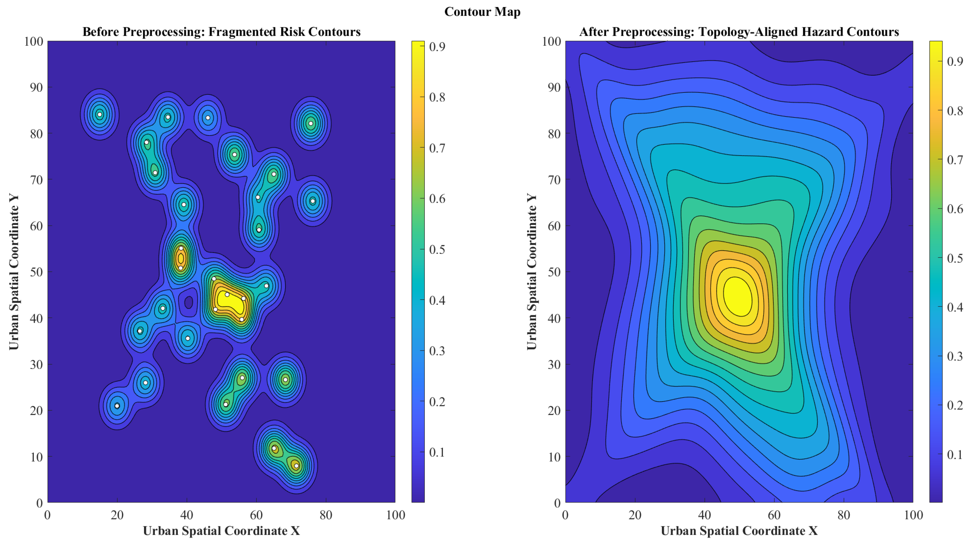
Temporal hold-outEarlier time periods are used for training, while later unseen periods are used for testing.Evaluates whether the model can predict future hazard states from past observations.Reduces temporal leakage and overly optimistic results caused by near-duplicate time-adjacent samples.
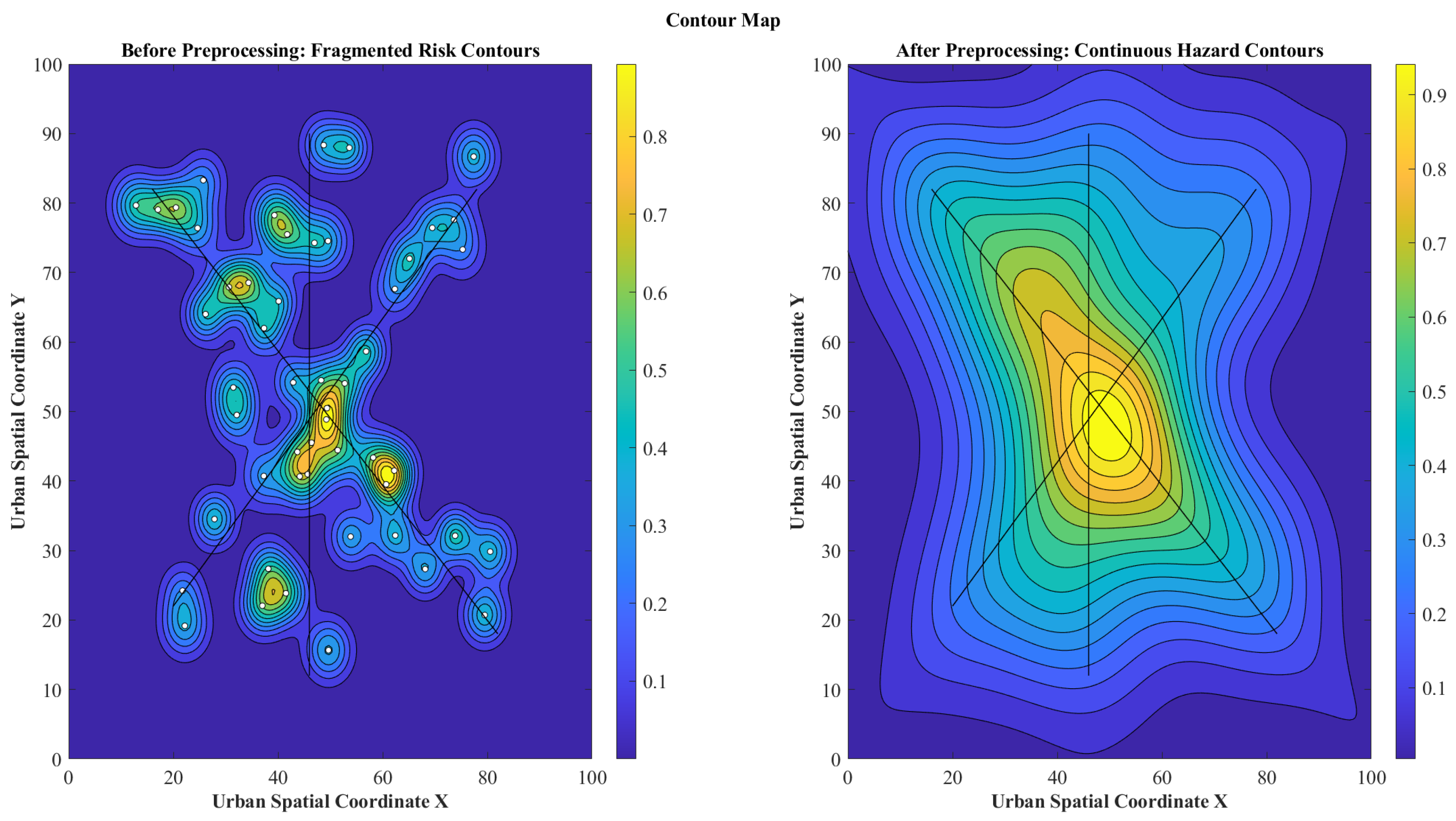
Geographic hold-outSelected corridors, regions, or spatial zones are excluded from training and used only for testing.Tests whether the learned hazard representation generalizes to unseen locations.Reduces spatial autocorrelation bias and location memorization.
Blocked spatio-temporal validationTraining and testing partitions are separated by both time and geographic units.Provides the strictest robustness check for spatio-temporal generalization.Controls simultaneous temporal dependence and spatial neighborhood overlap.
Table 14. Performance comparison under random, temporal hold-out, geographic hold-out, and blocked spatio-temporal validation settings.
DatasetValidation SettingAccuracyPrecisionRecallF1-Score
Dataset 1Stratified random split99.12%98.94%98.76%98.85%
Dataset 1Temporal hold-out97.84%97.51%97.28%97.39%
Dataset 1Geographic hold-out97.36%97.04%96.82%96.93%
Dataset 1Blocked spatio-temporal96.71%96.38%96.05%96.21%
Dataset 2Stratified random split98.63%98.41%98.16%98.28%
Dataset 2Temporal hold-out97.29%96.94%96.71%96.82%
Dataset 2Geographic hold-out96.88%96.52%96.19%96.35%
Dataset 2Blocked spatio-temporal96.14%95.78%95.43%95.60%
Table 15. Comparison with related traffic accident prediction studies and external baseline relevance.
StudyPrediction FocusModels/BaselinesKey EvidenceRelevance/Novelty
Park and Hong [14]Urban road-specific accident-risk prediction using static road, traffic, and environmental features.MLP model with different sampling ratios and feature combinations.Best balanced setting achieved accuracy = 0.75, precision = 0.73, and recall = 0.81.Supports MLP as a neural external baseline for urban accident-risk prediction.
Macedo et al. [15]Accident-frequency and severity prediction on rural highways using GIS and geometric road features.GEE model with negative binomial link and roadway  segmentation.Best model achieved QIC = 600.30; sharp curves showed 3.2 times higher accident risk.Highlights the value of spatial segmentation and roadway geometry, while CHFI extends this toward continuous spatio-temporal hazard reconstruction.
Gou et al. [16]Traffic-incident modeling using XTraffic with traffic-flow, speed, occupancy, incident, and roadway attributes.Decision Tree, TS2Vec, gMLP, Sequencer, OmniScaleCNN, PatchTST, and FormerTime.Incident classification reached about 41.6% accuracy in selected settings.Supports XTraffic-style incident modeling and motivates stronger external predictive baselines beyond internal variants.
Huang et al. [17]Traffic accident occurrence and severity prediction over road-network graphs.TRAVEL compared with MLP, XGBoost, and several GNN baselines.TRAVEL consistently outperformed non-graph and graph-based baselines.Directly supports adding XGBoost, MLP, and graph-based baselines.
Wang et al. [18]Intersection-level crash prediction using topology, traffic, weather, calendar, and risk features.LR, SVM, DT, RF, MLP, GCN, LSTM, and RoadInTCP.RoadInTCP achieved F1 = 0.8366–0.8694 and improved over baselines by 3.634–5.591%.Covers RF, MLP, LSTM, and graph-based GCN
Yumak et al. [19]Accident-severity classification and high-risk road-segment identification.LR, SVM, MLP, RF, and XGBoost.XGBoost achieved the best F1-score of 0.61 and lowest false-alarm rate of 0.01.Justifies RF, XGBoost, and MLP as strong external accident-severity baselines.
Li and Chen [13]Traffic accident-risk prediction using vehicle spatio-temporal trajectory data.Hybrid CNN, LSTM, and GNN architecture.Achieved accuracy = 94.5%, precision = 94.0%, recall = 93.7%, AUC = 0.978, and F1-score = 93.8%.Supports sequence-based and graph-based baselines such as LSTM/GRU and GNN.
Alnowaiser [20]Smart-city accident-severity prediction using geospatial, temporal, environmental, and vehicle-related factors.RF, LSTM, GRU, MLP, and GNN–LSTM–MLP with SHAP.Hybrid model achieved 99.97% accuracy and approximately 99.99% precision, recall, and F1-score.Directly supports comparison with RF, MLP, GRU/LSTM, and graph-sequential baselines.
Present CHFI studyContinuous urban hazard-field reconstruction and localized accident-emergence prediction using two large-scale traffic-safety datasets.Internal CHFI variants plus external baselines including RF, XGBoost, MLP, LSTM/GRU, and graph-based spatio-temporal models under the same experimental settings.Final CHFI achieved 99.12% accuracy, 98.85% F1-score, and 0.998 AUC on Dataset 1, and 98.63% accuracy, 98.28% F1-score, and 0.997 AUC on Dataset 2.Novelty lies in moving beyond discrete accident classification toward topology-aware continuous hazard-field learning, temporal hazard evolution, risk-diffusion lifting, hazard reconstruction, and localized accident-emergence inference.
Disclaimer/Publisher’s Note: The statements, opinions and data contained in all publications are solely those of the individual author(s) and contributor(s) and not of MDPI and/or the editor(s). MDPI and/or the editor(s) disclaim responsibility for any injury to people or property resulting from any ideas, methods, instructions or products referred to in the content.