Intelligent Optimization of Dry Machining for Machinability Enhancement of Super Duplex Stainless Steel

Abstract

Sustainable manufacturing increasingly demands environmentally friendly machining strategies, and dry machining has become recognized as a sustainable alternative to conventional coolant-assisted processes. This study presents a framework built on a machine learning technique for optimizing the dry machining performance of Super Duplex Stainless Steel (SDSS 2507) using textured cutting inserts. Gaussian process regression (GPR) models were developed to predict maximum roughness depth (R_max) and maximum flank wear (VB_max). Gaussian data augmentation was employed to enhance model generalization. The predictive performance was strong, with R² values recorded above 0.95 on testing datasets. To identify optimal machining parameters, GPR was integrated with particle swarm optimization (PSO), enabling independent optimization of R_max and VB_max. The framework achieved reductions of 13.97% in R_max and 30.70% in VB_max compared to experimental benchmarks. The results confirm the effectiveness of data-driven optimization in enhancing surface quality, tool performance, and intelligent machining control.

1. Introduction

Manufacturing has long been a driving force behind technological progress and industrial competitiveness, providing the foundation for producing components and systems with precise functionality and reliability. Among the various manufacturing approaches, machining remains one of the most essential processes due to its ability to generate accurate geometries and high-quality surfaces across a wide range of applications. Machining, as a subtractive process, makes products by material removal in the form of chips through the interaction between a cutting tool and a workpiece, enabling the creation of the functional surfaces required in sectors such as aerospace, automotive, and energy [1]. Despite the emergence of additive and hybrid manufacturing technologies, machining continues to play a central role in modern production systems because of its versatility, precision, and industrial maturity.

The increasing demand for advanced and high-performance materials has significantly amplified the challenges associated with machining processes. Among these, Super Duplex Stainless Steels (SDSS) stand out for their superior mechanical strength and enhanced corrosion resistance, making them indispensable in demanding sectors such as marine, nuclear, oil, and petrochemical industries [2]. However, these characteristics also make them difficult to machine, often leading to issues such as excessive tool wear, high cutting forces, work hardening, and compromised surface integrity [3]. These challenges are further intensified in dry cutting environments, where the elimination of cutting fluids to reduce environmental impacts places additional constraints on machining performance.

As a result, the optimization of machining parameters has become a critical research and industrial objective, as process conditions directly affect productivity, cost, and product quality [1]. Traditional approaches to process optimization, which rely heavily on empirical and analytical approaches and iterative experimentation, are often inefficient and costly. Analytical models typically depend on numerous simplifying assumptions that hinder their practical applicability. Moreover, such methods are limited in their ability to represent the complex, nonlinear associations among process variables and operational metrics in machining processes such as surface finish, cutting forces, and tool wear. Purely empirical methods frequently fail to deliver accurate and reliable predictions [4].

Historically, modeling in machining has been dominated by physics-based and analytical approaches that attempt to describe process behavior through simplified assumptions and mathematical formulations. While these models provide valuable insights into fundamental mechanisms, their predictive capability is often constrained by assumptions regarding system behavior and statistical distributions. In contrast, machine learning (ML) introduces a data-driven paradigm capable of capturing complex relationships directly from experimental and operational data. ML methods can process large volumes of information to uncover patterns and generate predictive models with greater flexibility and accuracy than conventional techniques, making them increasingly attractive for machining applications [5]. The integration of ML into manufacturing is closely aligned with the broader transition toward smart manufacturing and Industry 4.0. Data-driven approaches have opened new possibilities for designing intelligent frameworks for the descriptive, diagnostic, and predictive evaluation of machining processes. ML and deep neural techniques are now extensively applied for process monitoring, fault detection, and performance prediction, thereby enabling more informed and proactive decision-making in manufacturing environments [6]. In this context, intelligent machining emerges as a practical implementation of smart manufacturing, where sensor data, computational models, and analytics are integrated to enhance process understanding and control. Recent advancements associated with Industry 4.0 and Industry 5.0 have further accelerated the integration of artificial intelligence (AI) and ML in machining. These technologies contribute to the prediction of key process variables, such as cutting forces, cutting tool degradation, surface finish, and energy utilization, while also supporting the optimization of machining parameters. By enabling machines to extract patterns from data and adjust to dynamic operating conditions, ML-based systems improve productivity, extend tool life, and enhance overall part quality. This shift reflects a broader transformation from experience-based decision-making toward systematic, data-driven optimization in manufacturing [7]. From a methodological perspective, ML models are designed to capture the functional relations among process system inputs and responses without requiring explicit analytical formulations. Their performance is sensitive to the selected algorithms, training strategies, and evaluation metrics. Commonly applied ML techniques in machining research include support vector machines, artificial neural networks, decision tree methods, and regression-based approaches. Furthermore, data-driven optimization algorithms inspired by biological processes, including evolutionary approaches and particle swarm optimization, are increasingly employed to enhance machining performance and parameter selection [8]. Together, these developments underscore the growing importance of ML in modeling and optimizing machining processes, positioning it as a key enabler of next-generation manufacturing systems.

Numerous researchers have demonstrated machine learning applications and the integration of ML models in optimization frameworks. Some notable studies are discussed below.

Pimenov et al. [9] applied machine learning (ML) for the real-time prediction of average roughness ‘R_a’ in the face milling of carbon steel 45, using tool wear and main drive power as inputs. Without deploying additional sensors, the study aimed to improve productivity by compensating for tool wear-induced surface degradation. Among the tested models’ feed-forward layered perceptron system, RF (random forest), radial basis functions, and regression trees, RF achieved the highest accuracy, outperforming others by up to 44%. RF and regression trees also offered ease of tuning and interpretable outputs. Extending machine learning to complex optimization strategies, Yeganefar et al. [4] optimized the milling of Al alloy, employing ML modeling techniques, such as artificial neural network (ANN), and support vector regression (SVM), to predict surface roughness and cutting forces, followed by optimization with NSGA-II (a multi-objective evolutionary optimization algorithm). ANN outperformed SVM and regression; the ANN–NSGA-II hybridization approach effectively generated Pareto-optimal solutions, supporting improved machining efficiency and surface quality. Addressing sustainable machining goals, the Gupta et al. [10] study assessed the machinability of Ti alloy (grade II) in turning, using cubic boron nitride tools under nano-fluid assisted minimum-quantity lubrication (MQL), and developed predictive modeling frameworks constructed through an adaptive neuro-fuzzy inference system (ANFIS) and response surface methodology (RSM). ANFIS provided superior accuracy compared to the RSM. The Sizemore et al. [11] study evaluated machine learning and neural network models to predict surface roughness in single-point diamond turning of brittle germanium and ductile copper. Compared with analytical models, ML methods significantly improved prediction accuracy, especially for fracture-prone germanium. A deeper ANN architecture performed best overall, while classic ML models also showed strong results. Bhattacharya and Chakraborty [12] applied random forest to model CNC face milling using a small dataset of 27 experiments. The model predicted key output parameters, such as material removal rate, surface finish, and energy consumption, based on cutting parameters. Its performance, validated through multiple statistical metrics, demonstrated reliable predictive capability with minimal feature selection. The RF model showed robustness and flexibility for machining applications, although it was sensitive to out-of-range and sparse data. Notably, reliable predictions were achieved with relatively small datasets, highlighting ML’s practicality for costly precision machining applications. Machining forces, surface quality and cutting tool performance were predicted using Gaussian process regression (GPR) with cutting parameters as input variables in a study by Zhang and Xu [13]. The GPR models achieved high accuracy, stability, and robustness. This approach offers a fast, profitable, and reliable solution for estimating machining key performance, making it compatible with industrial applications and for broader use in CNC machining, to uncover correlations between process parameters and workpiece quality. The Korkmaz et al. [14] study applied machine learning to optimize machining quality by predicting tool wear under dry, MQL, and nano-MQL environments. Experiments on Bohler steel showed that MQL reduced flank wear by up to 25%, with hBN nano–MQL dual-spraying yielding the lowest wear. ML models closely matched real outcomes, with ridge regression and decision trees delivering the strongest predictive performance, enabling the data-driven selection of optimal eco-friendly machining conditions. The Jia et al. [15] study presented a staged energy prediction framework for CNC milling using a whale-optimized XGBoost model. The machining cycle was divided into four phases, each modeled separately to improve prediction stability and accuracy. The hybrid approach outperformed several benchmark algorithms and achieved about 95.5% accuracy. The results confirm that phase-based modeling combined with metaheuristic optimization provides a reliable tool for energy forecasting and supports more efficient, data-driven machining operations. The Bhowmik et al. [1] study evaluated gene expression programming (GEP), ANFIS, and neural networks for predicting key machining outcomes during the milling of Inconel 690. The models successfully captured nonlinear interactions among process parameters and responses such as surface quality, temperature, and cutting forces. Statistical testing confirmed high predictive accuracy, with GEP performing best overall. The results highlight machine learning as a practical alternative to trial-and-error optimization, offering improved efficiency and reliability in machining difficult superalloys and supporting smarter, data-driven manufacturing. In the realm of ultraprecision machining, Adizue and Takács [16] investigated the influence of the design of experiments on machine learning precision in the ultraprecision hard turning of AISI D2 steel. A BRNN model predicted surface roughness and MRR from cutting parameters using Taguchi and full factorial datasets. The full factorial design delivered superior prediction performance and supported a validated empirical model for real-time, data-driven process optimization. The Abbas et al. [3] study applied an XGBoost-based machine learning framework combined with MOORA and particle swarm optimization to improve the precision turning of AISI 4340 steel via conventional and wiper inserts. Experimental data were used to predict the surface roughness and material removal rate with high accuracy, which was further integrated with optimization algorithms. The results showed that feed and speed strongly influenced performance, while the wiper inserts delivered markedly smoother finishes. The hybrid optimization approach enhanced productivity, quality, and cost efficiency, with strong potential for broader manufacturing applications. Moyo et al. [17] optimized the ultra-fine grinding of low-grade copper sulfide ores using a hybrid RSM–ANN–ANFIS modeling framework to improve milling efficiency and reduce energy demand. The media filling ratio emerged as the key controlling factor, interacting strongly with speed and time. The optimization achieved substantial energy savings while maintaining target particle size. The model validation showed that ANFIS best predicted grind size and that ANN best estimated energy use, demonstrating the value of hybrid AI approaches for sustainable mineral processing. Nguyen et al. [18] proposed a hybrid data-driven framework for optimizing the dry turning of AA6063 by balancing surface roughness and material removal rate. A Kolmogorov–Arnold network delivered the best predictive accuracy and interpretability among the tested ML models. Integrated with NSGA-III and MCDM ranking, it generated and prioritized Pareto-optimal cutting conditions. The approach supports rational parameter selection and demonstrates the effectiveness of combining interpretable machine learning with multi-objective optimization in machining. An important study by Pashmforoush et al. [19] introduced a Bayesian optimization framework combined with Gaussian process regression to improve milling productivity under multiple industrial constraints. The method simultaneously maximized material removal rate and minimizes machining cost while enforcing limits on power, torque, chatter, form error, and tool life. A physics-informed ML force model reduced experimental data needs, and Shapley-based sensitivity analysis added interpretability. The hybrid strategy achieved 18–26% performance gains, demonstrating reliable, scalable optimization for smart manufacturing. The Elly et al. [20] study developed surrogate ANN models and a genetic algorithm framework to minimize burr formation in the micro-milling of hardened AISI H13. Sensor-based experimental data were used to build interpretable ANN predictors with over 90% accuracy. The surrogate ANN, integrated with multi-objective GA, reduced burr sizes by about 35% and identified optimal cutting conditions. Compared with RSM-based optimization, the hybrid ANN approach delivered superior performance, supporting efficient, AI-driven burr control in precision micromachining. The Yin et al. [21] study integrated a multi-point thin-film thermocouple array with machine learning to monitor milling tool temperature and wear. A dual-regression XGBoost model predicted thermal behavior and wear with high accuracy using sensor-driven experimental data. The array captured spatial heat gradients linked to wear evolution, overcoming single-point limitations. The results showed that cutting speed and depth dominate thermal damage. The framework supports predictive tool monitoring and adaptive process optimization in high-performance machining.

Overall, recent studies in the literature demonstrate a clear shift toward integrating machine learning with advanced optimization frameworks to address complex machining trade-offs. Hybrid models combining ANN, XGBoost, GPR, and neuro-fuzzy systems with evolutionary and Bayesian optimization consistently improve prediction accuracy, energy efficiency, surface finish, and tool performance. These studies highlight the value of interpretable, data-driven models for multi-objective decision-making under industrial constraints. Collectively, the reviewed work confirms that ML-guided optimization is becoming a cornerstone of intelligent, sustainable, and adaptive manufacturing systems.

During the production of SDSS components, machining operations are critical for achieving precise geometries and dimensional accuracy. Despite their advantageous properties, SDSS components present significant challenges in terms of machinability [3]. These challenges are primarily attributed to their low thermal conductivity, a strong tendency for built-up edge (BUE) formation, and pronounced work-hardening behavior [22]. Such characteristics complicate machining operations by increasing tool wear, heat generation, and surface irregularities, necessitating advanced strategies to achieve optimal results.

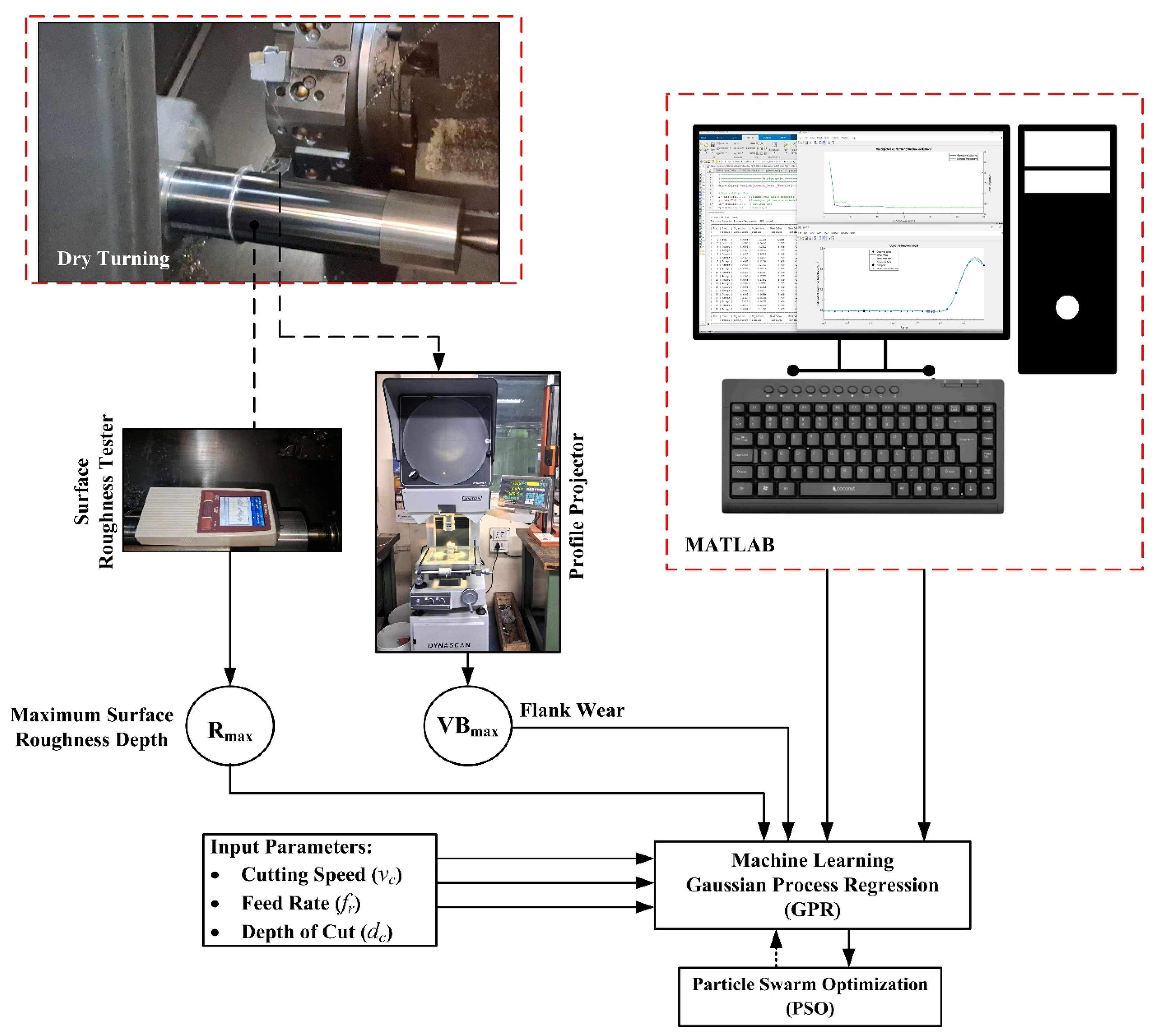
In view of these material-specific challenges and building on machine learning–based optimization insights reported in the literature, this study models machinability indicators—specifically, the maximum surface roughness (R_max) and flank wear (VB_max) during the dry turning of SDSS 2507 using textured cutting tools. The tools incorporate dimple, groove, and wave patterns on the flank face. The adoption of textured tools is driven by their proven potential to enhance overall machining effectiveness [23]. Separate machine learning models for each response (R_max and VB_max) are developed using Gaussian process regression. The developed model is evaluated using multiple statistical metrics and validated on an unseen dataset to ensure robustness. Following the modeling phase, the predictive framework is integrated with particle swarm optimization (PSO) to identify optimum process parameters for each machining response, namely R_max and VB_max. The findings are expected to fulfil research gaps by supporting an intelligent control framework for process management and improving the machining performance of SDSS components.

2. Materials and Methods

The overall procedure and methodological sequence of the proposed approach are outlined in Figure 1. Experiments were conducted on grade 2507 Super Duplex Stainless Steel, which was selected because of its outstanding mechanical strength and resistance to corrosive environments. The cutting setup employed CNMG 120408 45 DP5010 carbide inserts with TiAlN PVD coating, which were secured in an ISO-compliant tool holder of MCLNL 2525 M12. Turning experiments were conducted using a Super Jobber 500 CNC lathe supplied by Ace Micromatic, incorporating a 7.5 kW spindle unit. The machining was conducted under dry conditions, where cutting fluids were not used in order to reduce environmental impacts. To enhance machining performance, textured cutting inserts were employed, featuring three textured geometries characterized by groove, dimple, and wave themes in discrete, as well as continuous, arrangements. Surface texturing was produced with a femtosecond Nd:YAG laser system over a 2.5 mm × 2.5 mm region of the flank face, leaving an untreated clearance zone of approximately 150 μm adjacent to the tool nose radius. Texture dimensions (diameter/width = 50 μm, depth = 50 μm) were maintained uniformly, with an inter-texture spacing of 150 μm. Each experiment used a fresh cutting insert. A 1064 nm wavelength laser was employed to texture the cutting tool surface. The laser was operated at a repetition frequency of 3 kHz and a power level of 3 W, while the scanning velocity was maintained at 100 mm/s to ensure consistent and reproducible formation of the desired surface textures.

Experiments followed a Taguchi L₂₇ fractional orthogonal array, systematically varying machining speed, feed rate, and cutting depth as continuous factors together with the selected texture design as categorical factor. All the process parameters were varied at three levels: cutting speed (75–100–125 m/min); feed rate (0.06–0.12–0.18 mm/rev); and depth of cut (0.4–0.8–1.2 mm). Surface roughness was quantified using maximum roughness depth (R_max), which represents the maximum peak-to-valley height across the sampling length. R_max was chosen owing to its responsiveness to severe surface deviations that strongly influence functional performance evaluation. To ensure measurement accuracy, three R_max readings were measured at equal angular positions with a Mitutoyo SJ-210 roughness measurement tester, adhering to ISO 1997 standards [24]. This rigorous approach ensured reliability, reproducibility, and consistency in the surface roughness data. Flank wear (VB_max) was quantified with a high-precision optical device, the Dynascan PT 440 Neo profile projector, which provides a minimum measurement resolution of 0.001 mm. Detailed information on the tool wear measurement can be found in Pawanr and Gupta [25]. The measured values of R_max and VB_max, corresponding to the Taguchi L₂₇ fractional orthogonal array, are illustrated in Figure 2.

3. Overview of Modeling and Optimization Techniques

3.1. Modeling Technique: Gaussian Process Regression

Gaussian process regression (GPR) is a non-parametric Bayesian regression technique that enables the modeling of intricate and nonlinear dependencies between input and output variables with high flexibility. Unlike traditional parametric models, which assume a predefined functional form (e.g., linear or polynomial) and estimate a fixed set of parameters, GPR defines a probabilistic distribution over functions that could have generated the data [13,26]. This flexibility enables GPR to adapt to a wide range of functional relationships based on the observed data.

Formally, a Gaussian process (GP) can be described as a stochastic framework in which any finite subset of variables follows a multivariate Gaussian distribution. The behavior of a GP is completely characterized by its mean function, $\mu \left(z\right)$, and covariance function, $C(z,z^{*})$, which define its statistical properties, and are defined as [27,28]:

$$\mu \left(z\right)=E\left[f\right(z\left)\right]$$

$$C(z,z^{*})=E[\left(f\left(z\right)-\mu \left(z\right)\left(f\left(z^{*}\right)-\mu \left(z^{*}\right)\right)\right].$$

Thus, the prior distribution over functions can be written as:

$$f\left(z\right)~GP\left(\mu \left(z\right),C\left(z,z^{*}\right)\right).$$

The choice of covariance function $C(z,z^{*})$ is critical in GPR, since it captures prior assumptions regarding the smoothness, periodic behavior, and other characteristics of the target function. Commonly used kernels include the squared exponential (RBF) kernel and the Matérn kernel [28].

In this study we used the RBF kernel shown below:

$$C(z,z^{*})={\sigma }_s^2\mathrm{e}\mathrm{x}\mathrm{p}\left(-{\displaystyle \frac{{‖z-{\mathrm{z}}^{*}‖}^2}{2l_c^2}}\right)$$

where ${\sigma }_s^2$ denotes the signal variance and $l_c$ represents the characteristic length scale.

Let the training samples be represented as $\left\{\right(Z,y\left)\right\}$, where $Z={\left[z_1,z_2,...,z_n\right]}^T$ are the input vectors and $y={\left[y_1,y_2,...,y_n\right]}^T$ are the corresponding outputs; GPR models the combined distribution over the observed outputs and the prediction for a new input $z^{\prime }$ as:

$$\left[\begin{array}{c}y\\ y^{\prime }\end{array}\right]~N\left(0,\begin{array}{cc}C(Z,Z)+{\sigma }_n^{2}I& C(Z,z^{\prime })\\ C(z^{\prime },Z)& C(z^{\prime },z^{\prime })\end{array}\right)$$

where ${\sigma }_n^2$ represents the noise variance and C$(.,.)$ denotes the covariance matrices between points. Using the properties of multivariate Gaussian distributions, for a new input location $z^{\prime }$, the resulting predictive distribution is Gaussian and is formulated as:

$$y^{*}|Z,y,z^{\prime }~N({\mu }^{\prime },Var\left(y^{\prime }\right))$$

where the mean prediction is

$${\mu }^{\prime }=C\left(z^{\prime },Z\right){\left[C\left(Z,Z\right)+{\sigma }_n^{2}I\right]}^{-1}y$$

and the variance (uncertainty) prediction is

$$Var\left(y^{*}\right)=C\left(z^{\prime },z^{\prime }\right)-C\left(z^{\prime },Z\right){\left[C\left(Z,Z\right)+{\sigma }_n^{2}I\right]}^{-1}C\left(Z,z^{\prime }\right).$$

This provides not only a point estimate but also a confidence interval around each prediction, enabling users to assess the reliability of the model’s outputs. Another key feature of GPR is its natural handling of observational noise. By explicitly modeling the noise variance, GPR ensures robust predictions even in the presence of measurement errors or stochastic effects [28]. Overall, Gaussian process regression offers a principled and interpretable approach for regression tasks where uncertainty quantification and flexibility are critical. Its probabilistic formulation, ability to capture complex patterns, and built-in uncertainty estimation make it well suited to a wide range of scientific and engineering applications. Figure 3 outlines the flow of the proposed GPR model.

3.2. Optimization Technique: Particle Swarm Optimization (PSO)

Particle swarm optimization (PSO), a widely used metaheuristic method, is motivated by the cooperative social dynamics of biological swarms. PSO is particularly well-suited for addressing complex optimization problems due to its simplicity, efficiency, and ability to explore large search spaces effectively [3]. PSO operates by enabling a set of particles, each encoding a candidate solution, to move through the solution space via velocity-driven position updates. The position of each particle is iteratively modified by considering both the particle’s historically best solution and the collective optimum discovered by the swarm [26,29]:

$$m_i(k+1)=w\cdot m_i\left(k\right)+{\phi }_1\cdot {\eta }_1\cdot (s_j-z_j(t\left)\right)+{\phi }_2\cdot {\eta }_2\cdot (s^{*}-z_j\left(k\right))$$

$$z_j(k+1)=z_j\left(k\right)+m_j\left(k+1\right)$$

where $z_j$ and $m_j$ represent the position and velocity of particle j at iteration k; $w$ is the inertia weight; ${\phi }_1$ and ${\phi }_2$ are acceleration coefficients; ${\eta }_1,{\eta }_2\in [0,1]$ are uniformly distributed random numbers; and $s_j$ and $s^{*}$ represent personal and global best positions. This balance of exploration and exploitation facilitates efficient convergence toward global optima, particularly in high-dimensional and non-convex search spaces. The operational framework of the proposed PSO approach is outlined in Figure 4.

4. Results and Discussion

4.1. Implementation of Gpr

In this study, Gaussian process regression was employed to model the maximum roughness depth (R_max) and flank wear (VB_max) based on machining parameters. Four process parameters were used as model inputs: machining speed, feed, cutting depth, and surface texturing condition. The texturing parameter represents a qualitative factor composed of three geometry classes, dimple, groove, and wave, which were incorporated into the model as discrete categorical levels. R_max and VB_max served as the response variables characterizing surface finish and tool wear performance.

To enhance model accuracy and mitigate overfitting, Gaussian data augmentation (GDA) was applied [30,31], expanding the original 27 sample dataset to 81 samples for modelling both responses, R_max and VB_max. Two augmented samples per original sample were obtained by introducing controlled Gaussian noise into the continuous parameters, with noise levels set at 5% of each variable’s range. The 5% Gaussian noise level was selected to enrich the local data space while preserving the underlying characteristics of the experimental observations. This moderate perturbation helps to introduce variability into the limited dataset without causing substantial deviation from the original data distribution. The selection of a 5% perturbation level is supported by previous research and empirical evidence [32,33], indicating its suitability for enhancing data diversity while preserving the physical and statistical characteristics of the original dataset. The texture category was kept constant to maintain classification consistency. The data were partitioned, with 80% used for training and 20% reserved for model evaluation, with 65 training samples and 16 test samples selected to ensure balanced representation across variables. To optimize model learning, data normalization was applied. Continuous features were standardized using the standard scaling technique (zero mean, unit variance), while the texture type was transformed through one-hot encoding to ensure compatibility with machine learning algorithms.

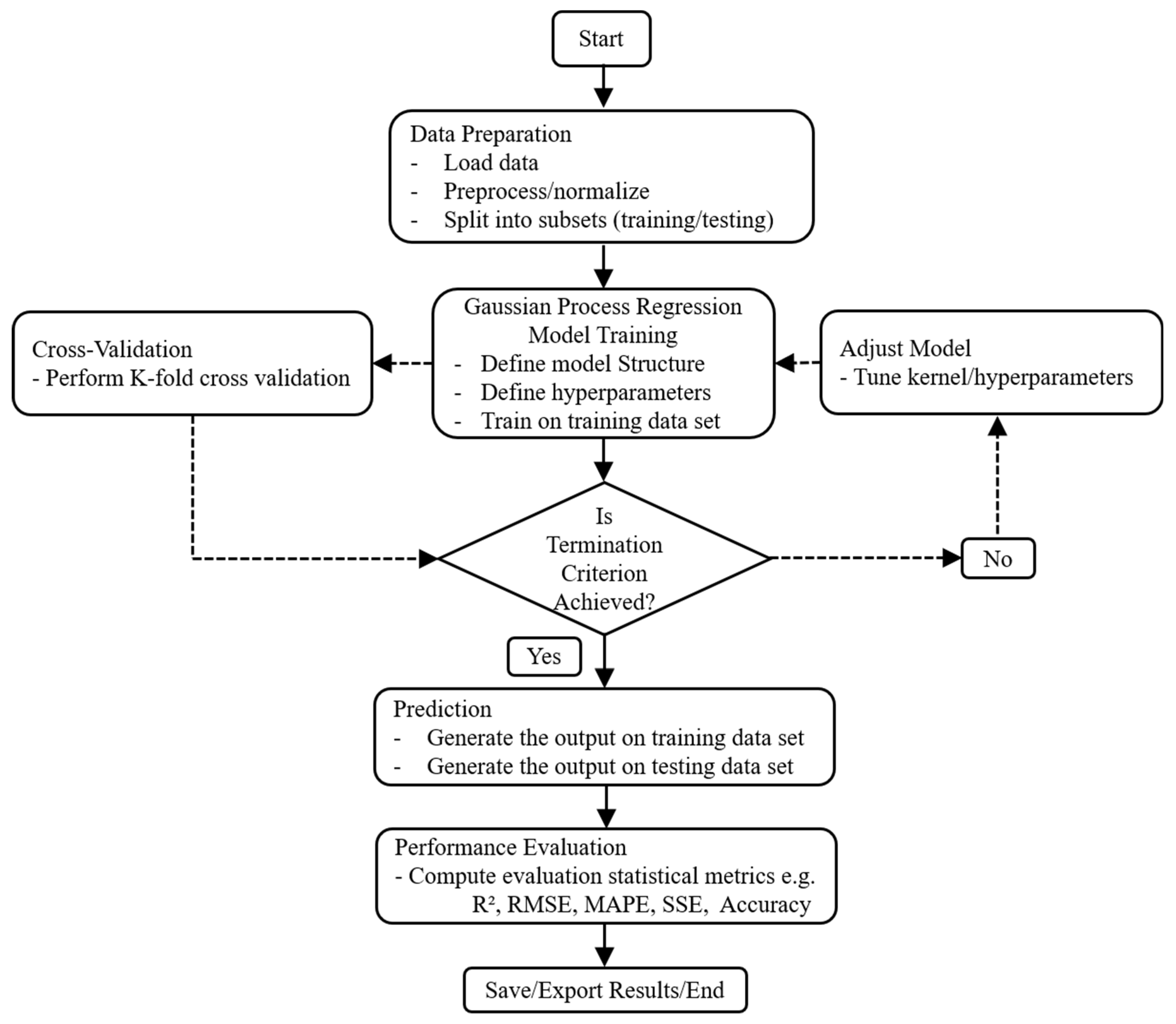
Gaussian process regression (GPR) models for R_max and VB_max were trained under a common configuration. GPR was implemented using the MATLAB R2021a fitrgp function. The covariance structure was defined using a squared exponential kernel, selected for its effectiveness in capturing smooth and nonlinear patterns in the data. The texture type was incorporated through one-hot encoding; therefore, the squared-exponential kernel treats the three texture categories as distinct states with equal separation in the encoded space. However, this representation does not explicitly capture physical similarities between texture geometries. A compound kernel with a dedicated categorical component could provide a more flexible representation, although its additional kernel components and hyperparameters may increase model complexity. The initial noise standard deviation (Sigma) was set to 0.1. Sigma (${\sigma }_n$) represents the standard deviation of the Gaussian observation noise in the GPR model. It quantifies the random noise or measurement variability present in the target response data. To enhance model performance, automatic hyperparameter optimization was enabled (OptimizeHyperparameters = ‘auto’), enabling the optimization of kernel parameters and noise level. The Bayesian optimization process used the “expected-improvement-plus” acquisition function to efficiently search the hyperparameter space. Furthermore, a five-fold cross-validation procedure was conducted to assess the generalization capability of the trained GPR model and minimize the risk of overfitting. These parameter settings collectively ensured a robust and accurate implementation of the GPR model for the prediction task in this research.

Table 1. Initial training configuration of the GPR models.

Setting	Value
Model type	Gaussian Process Regression (fitrgp)
Kernel function	Squared exponential
Input preprocessing	Standardized inputs
Initial sigma	0.1
Hyperparameter optimization	Expected-improvement-plus
Cross-validation	5-fold CV (kfoldLoss)
Total optimization iterations	30

summarizes the initial training configuration of both models, while

Table 2. Summary of GPR model optimization metrics.

Metric	GPR Model
	Rmax	VBmax
Best observed objective value	1.4393	5.0123
Best estimated objective value	1.4394	5.0122
Sigma (${\sigma }_n$) (best observed)	0.7247	2.1297
Sigma (${\sigma }_n$) (best estimated)	0.7244	2.0238
Best objective evaluation time (s)	0.0861	0.10627
Total elapsed time (s)	19.701	26.3668
Total objective evaluation time (s)	3.1513	4.603
Cross-validated RMSE	1.2681	9.6275

presents the optimization outcomes and performance metrics for the two models. Although both models follow identical training settings, their optimal hyperparameters and objective values differ, reflecting the distinct response characteristics of R_max and VB_max.

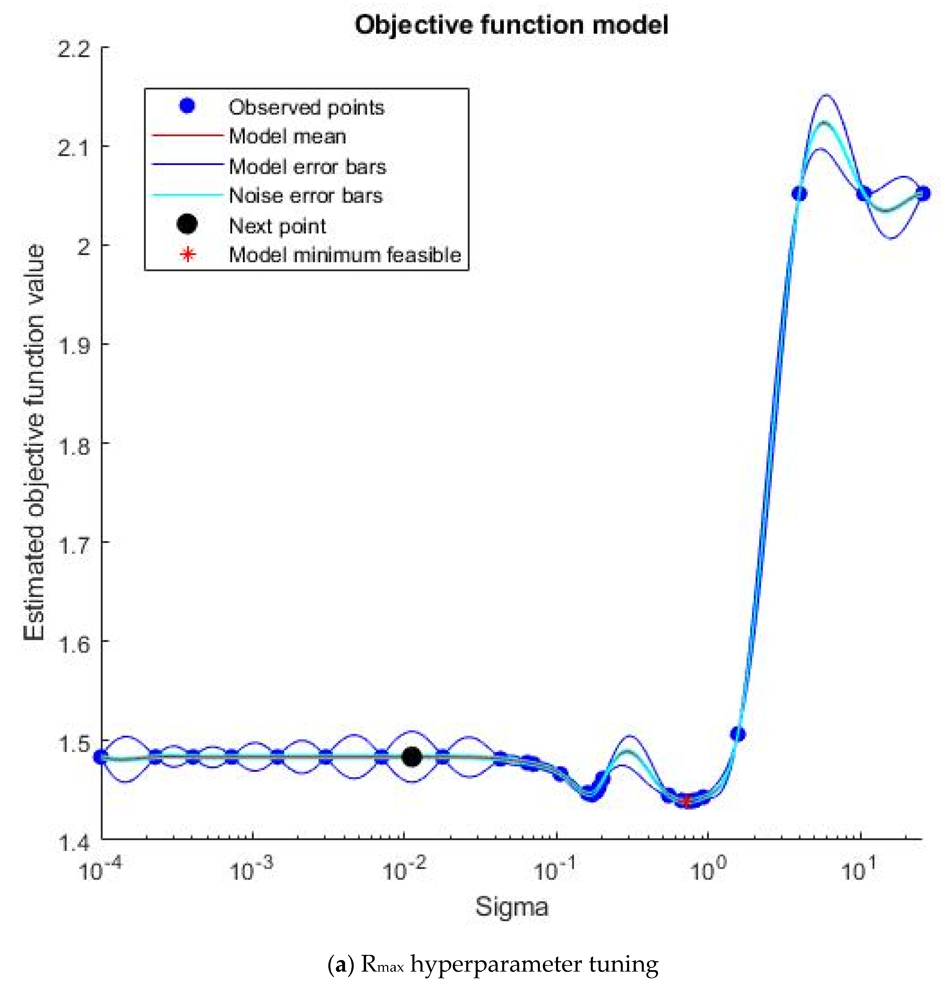
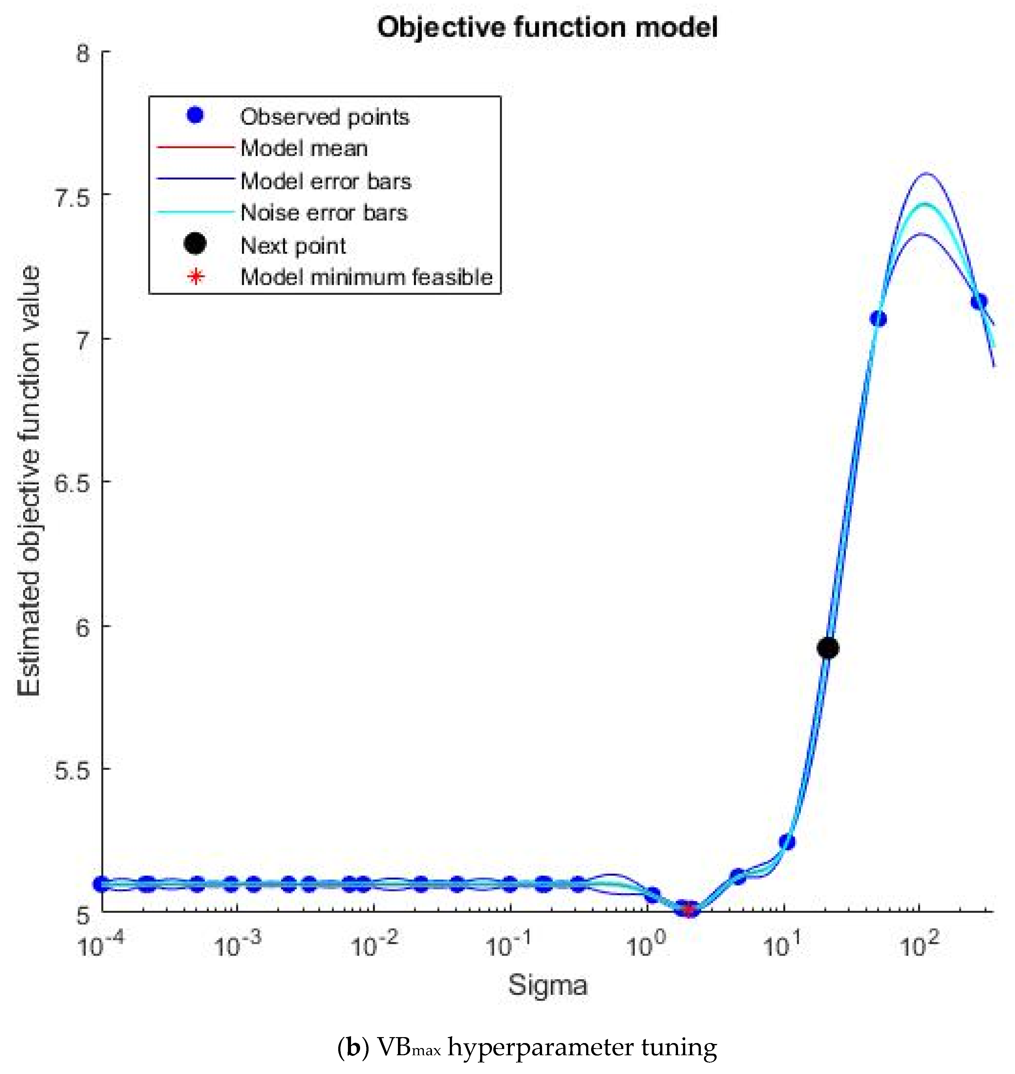
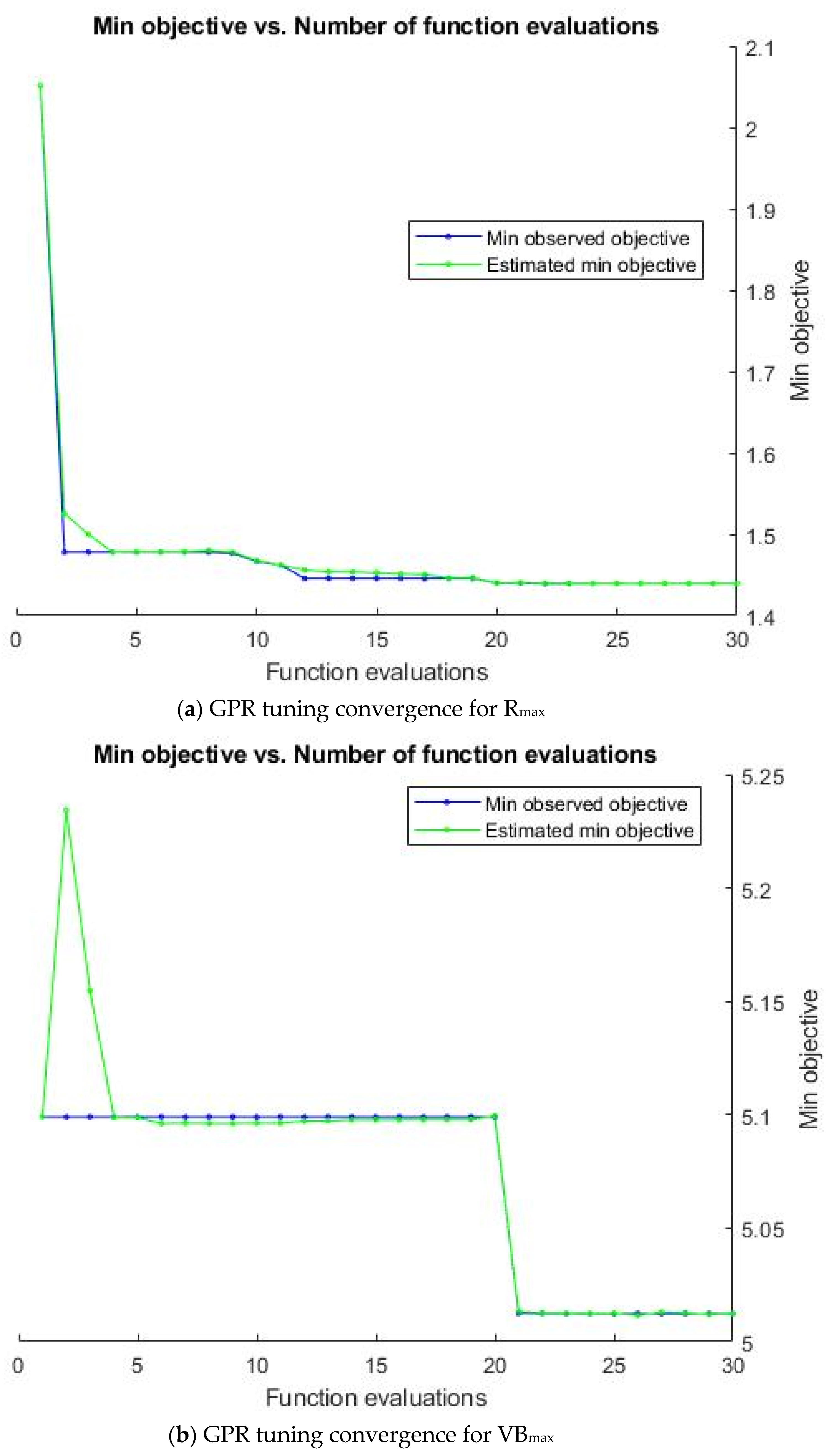
Figure 5a and Figure 5b illustrate the convergence trajectories of the Bayesian optimization processes used to calibrate the hyperparameters of the GPR models developed for R_max and VB_max, respectively, showing the minimum observed and estimated minimum objective values as a function of the number of function evaluations. In each case, the optimization objective was minimized over 30 evaluations by adjusting the noise standard deviation (${\sigma }_n$) within the squared exponential kernel GPR framework. The early iterations exhibited noticeable variability in the objective values, reflecting the exploratory phase of the optimization. As the search progressed, both trajectories stabilized, indicating convergence toward model-specific optimal configurations. For the R_max model, the minimum observed objective value of 1.4393 was reached with ${\sigma }_n$ ≅ 0.7247, whereas the VB_max model converged to a minimum observed objective value of 5.0123 at ${\sigma }_n$ ≅ 2.1297. These trends confirmed the stable convergence behavior of the Bayesian optimization procedure for both response models.

Figure 6a and Figure 6b depict the iterative refinement of the observation-noise standard deviation (${\sigma }_n$), labeled “Sigma” on the horizontal axis, during the Bayesian optimization of the GPR models for R_max and VB_max, respectively. The figures show the estimated objective function value against the explored values of ${\sigma }_n$. Each evaluation point represents a tested hyperparameter configuration and its associated objective value, providing a visual record of how the optimizer navigates the parameter space. Complementary to the convergence plots, these figures illustrate the balance between the exploration of uncertain regions and the exploitation of promising configurations that characterizes Bayesian optimization.

In both models, the concentration of low-objective regions around the final ${\sigma }_n$ values indicate stable identification of near-optimal hyperparameters. The optimized ${\sigma }_n$ values differed between R_max and VB_max because the two responses exhibit different levels of variability arising from their distinct physical characteristics. R_max is affected by instantaneous tool–workpiece interactions, chip formation, feed-induced surface generation, and tool geometry, whereas VB_max represents an accumulated wear response involving thermal, mechanical, abrasive, and adhesive effects. These differences can result in distinct nonlinear behavior and experimental variability, leading to different optimized ${\sigma }_n$ values. The observed search patterns demonstrate consistent optimizer behavior and confirm the effectiveness of Bayesian optimization as a calibration strategy for the GPR framework. Together, these figures highlight the structured progression of the tuning process and the robustness of the resulting model configurations.

4.2. GPR Model Performance Evaluation

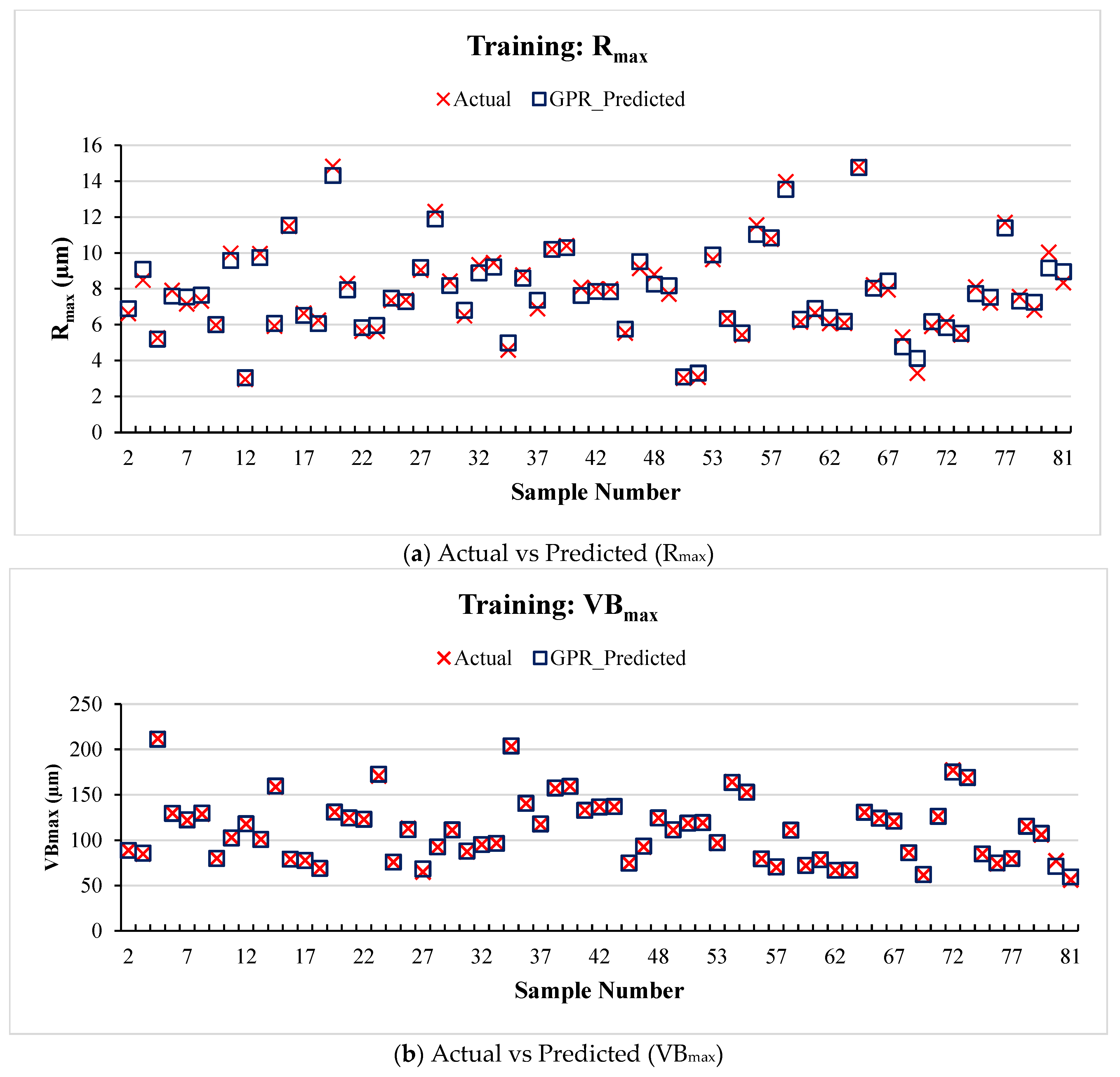
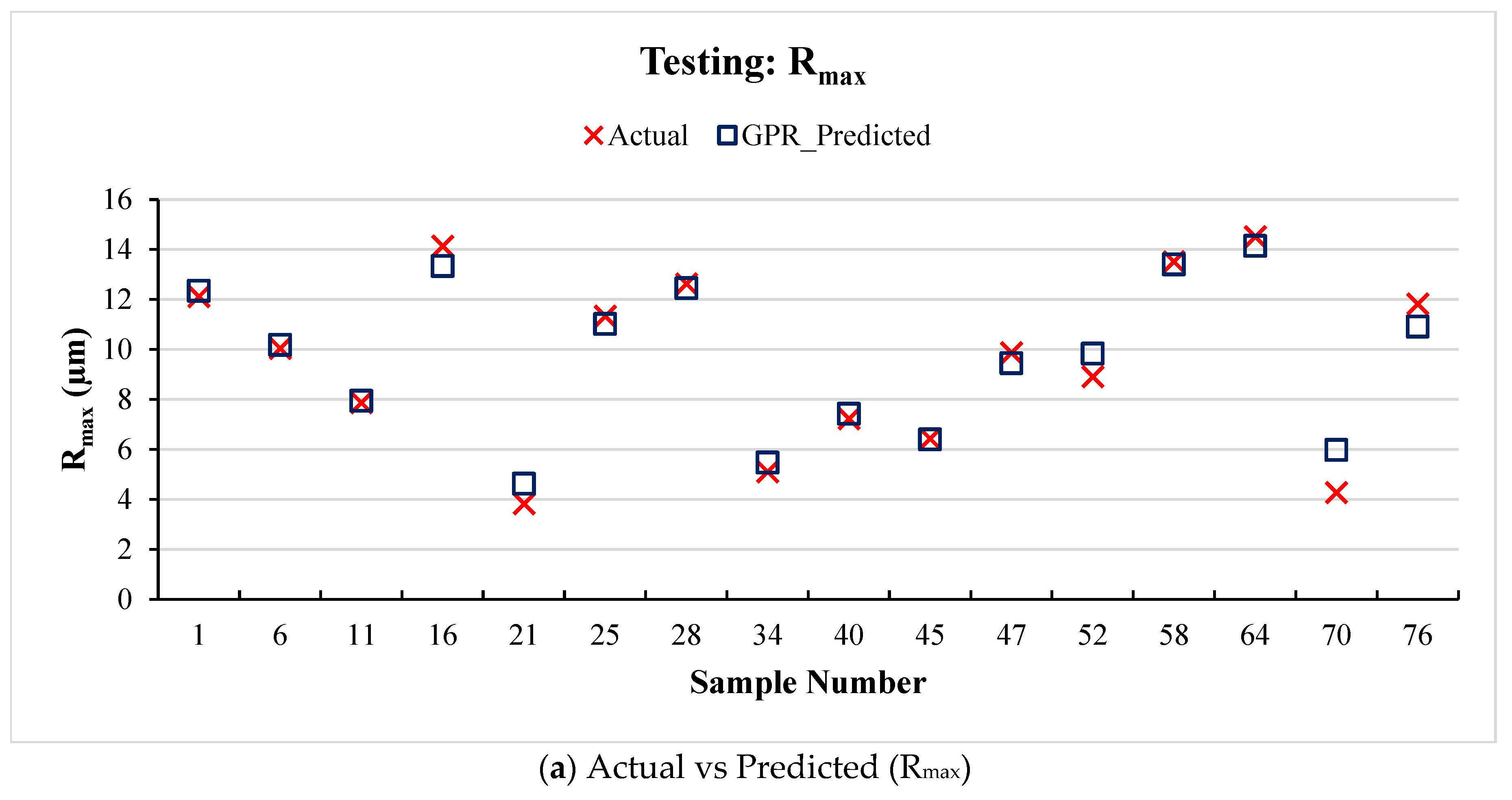
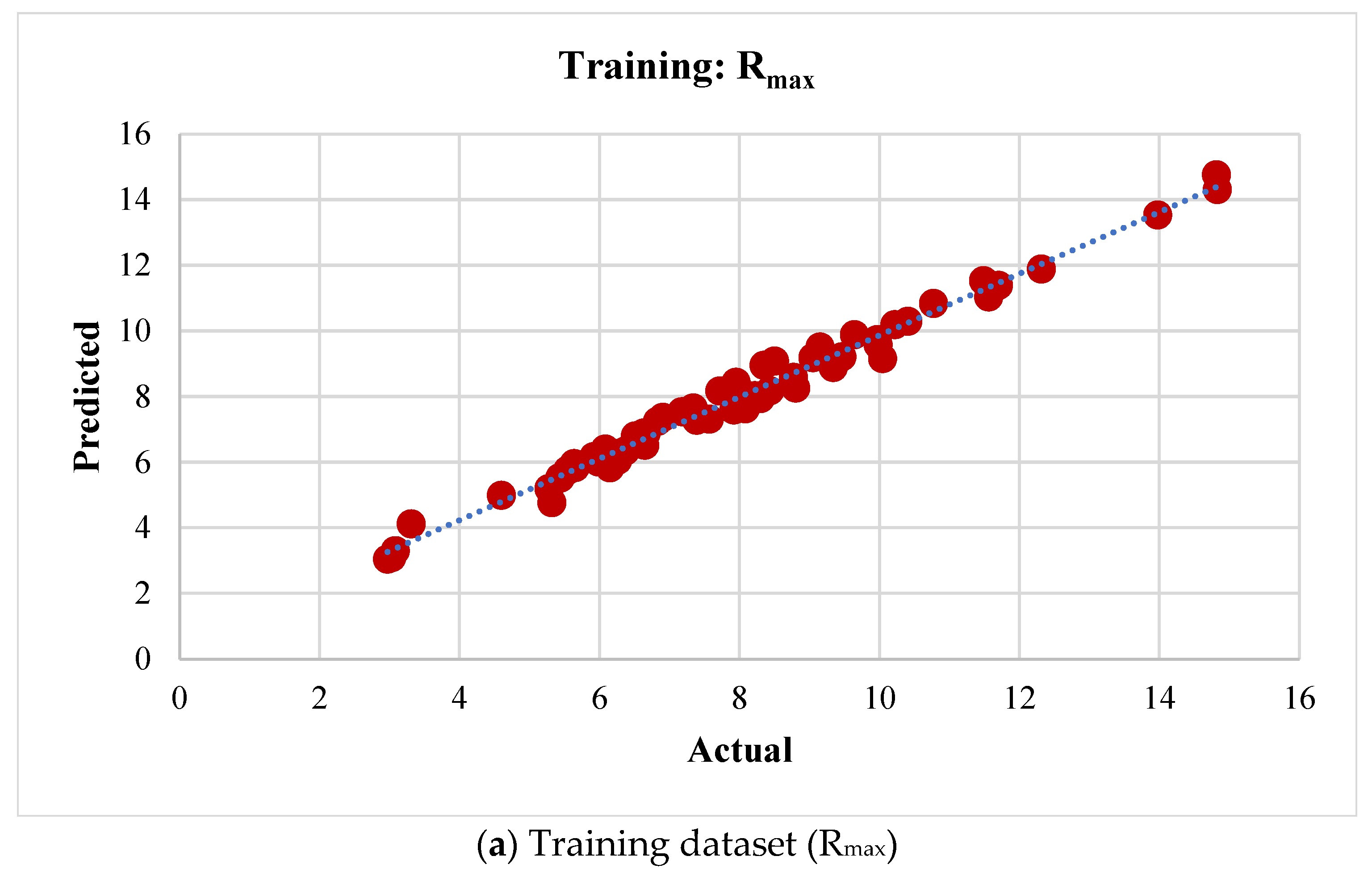
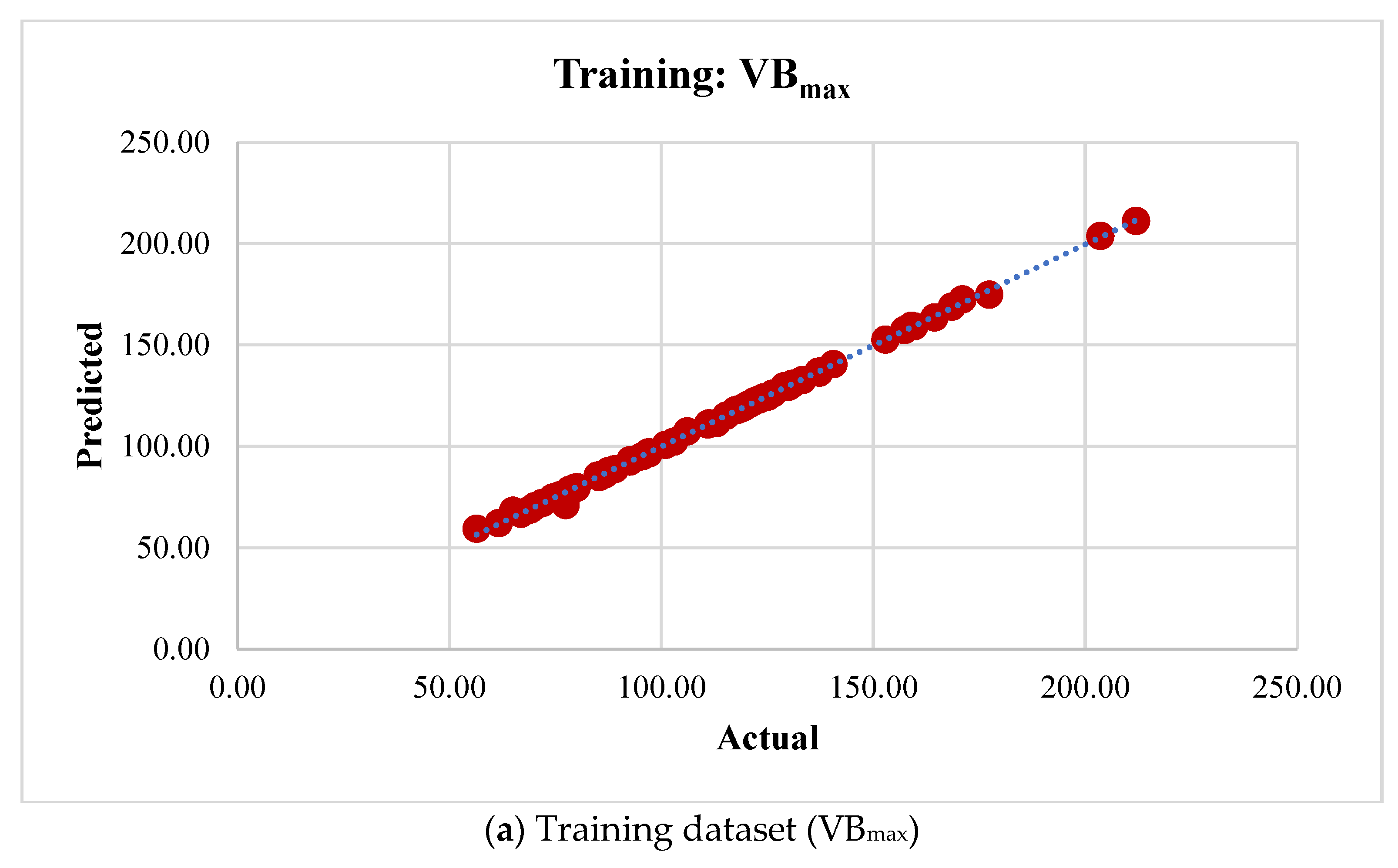
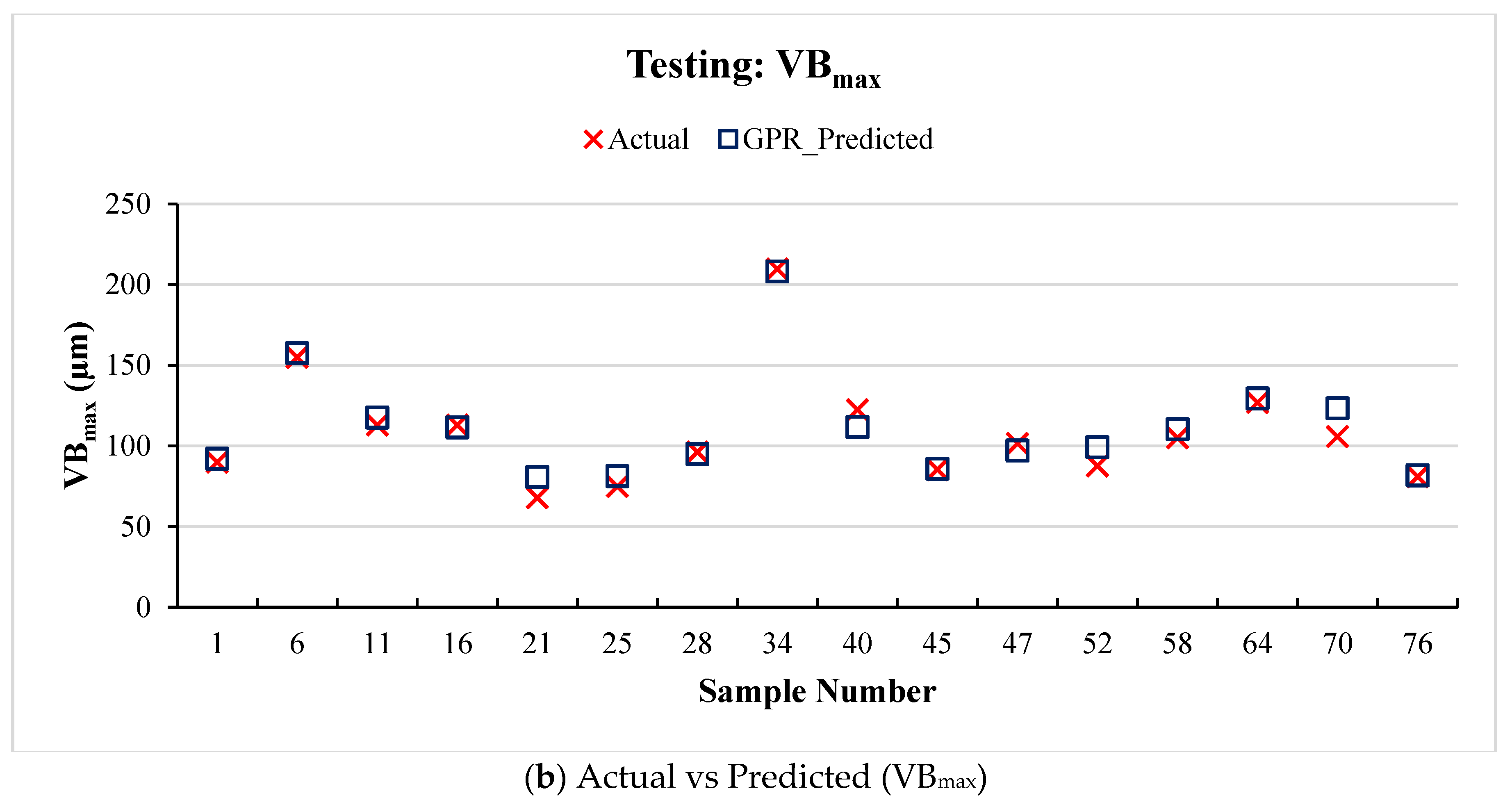
The predictive performance of the Gaussian process regression (GPR) framework was evaluated by examining the agreement between actual and predicted values for both R_max and VB_max across the training and testing datasets in Figure 7 and Figure 8, respectively.

As illustrated in Figure 7a, the GPR model establishes a robust agreement between the predicted and experimental R_max values during the training phase, indicating its ability to accurately acquire the complex nonlinear relationships present in the data. This close alignment reflects the model’s high accuracy combined with robust learning capability. Similarly, Figure 7b show that the GPR model for VB_max exhibits comparable agreement between predicted and actual values during training, confirming its effectiveness in modeling the response behavior.

Furthermore, the models maintain this performance when applied to the respective testing datasets. As shown in Figure 8a,b, the overall predictive patterns reflect similar tendencies observed in the training phase, confirming reliable generalization to unseen data for both responses. The present findings validate the efficacy of the GPR framework in modeling R_max and VB_max, underscoring its practical applicability in real-world machining processes.

In addition, the predictive capability of the GPR was subjected to comprehensive evaluation through a comprehensive set of statistical performance metrics. Among the evaluation metrics was the coefficient of determination (R²), which measures how much of the variability in the response variable is accounted for by the model, shown in Equation (1); the sum of squared errors (SSE), which captures the total discrepancy between model predictions and observed values, shown in Equation (2); the mean squared error (MSE) and its square root, the root mean squared error (RMSE), both of which measure the average magnitude of prediction errors and are shown in Equations (3) and (4), respectively; the mean absolute error (MAE), which measures the average absolute deviation between predicted and observed values, shown in Equation (5); and the mean absolute percentage error (MAPE), which expresses prediction accuracy as a percentage, shown in Equation (6). Together, these metrics offer a detailed and robust accuracy evaluation of the model, consistency, and generalization performance across training and testing datasets. The following mathematical formulas were used to calculate the quantitative performance metrics:

$${\mathrm{R}}^2=1-\left({\displaystyle \frac{\sum {\left(y_{\mathrm{i}}-{\widehat{y}}_{\mathrm{i}}\right)}^2}{\sum {\left(A_{\mathrm{i}}-\overline{A}\right)}^2}}\right)$$

(1)

$$\mathrm{S}\mathrm{S}\mathrm{E}={\sum }_{i=1}^s{\left(y_{\mathrm{i}}-{\widehat{y}}_{\mathrm{i}}\right)}^2$$

(2)

$$\mathrm{M}\mathrm{S}\mathrm{E}={\displaystyle \frac{1}{\mathrm{s}}}{\sum }_{i=1}^s{\left(y_{\mathrm{i}}-{\widehat{y}}_{\mathrm{i}}\right)}^2$$

(3)

$$\mathrm{R}\mathrm{M}\mathrm{S}\mathrm{E}=\sqrt{{\displaystyle \frac{{\sum }_{i=1}^s{\left(y_{\mathrm{i}}-{\widehat{y}}_{\mathrm{i}}\right)}^2}{s}}}$$

(4)

$$\mathrm{M}\mathrm{A}\mathrm{E}={\displaystyle \frac{{\sum }_{i=1}^s|y_{\mathrm{i}}-{\widehat{y}}_{\mathrm{i}}|}{s}}$$

(5)

$$\mathrm{M}\mathrm{A}\mathrm{P}\mathrm{E}={\displaystyle \frac{100}{s}}\%\times {\sum }_{i=1}^s\left|{\displaystyle \frac{y_{\mathrm{i}}-{\widehat{y}}_{\mathrm{i}}}{y_{\mathrm{i}}}}\right|.$$

(6)

Here, $s$ represents the total number of observations (samples), and $y_i$ and ${\widehat{y}}_i$ represent the measured values and GPR estimated values, respectively. The computed values of R², SSE, MSE, RMSE, MAE, and MAPE for the GPR model evaluated on the training, as well as the testing sets, are reported in

Table 3. Statistical results for the GPR model evaluation on the training dataset.

GPR Model	Metrics
	R2	RMSE	MAPE	SSE	MSE	MAE
Rmax	0.982	0.339	3.962	7.482	0.115	0.284
VBmax	0.999	1.104	0.613	79.257	1.219	0.563

and

Table 4. Statistical results for the GPR model evaluation on the testing dataset.

GPR Model	Metrics
	R2	RMSE	MAPE	SSE	MSE	MAE
Rmax	0.964	0.642	6.979	6.605	0.413	0.474
VBmax	0.953	7.267	5.588	844.933	52.797	5.343

, respectively.

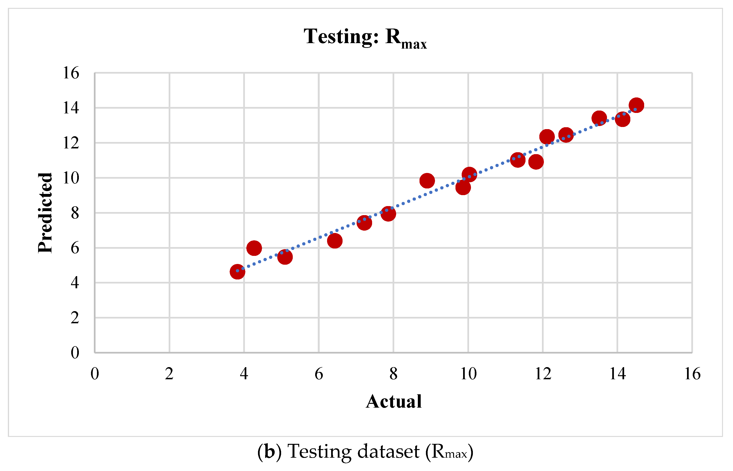
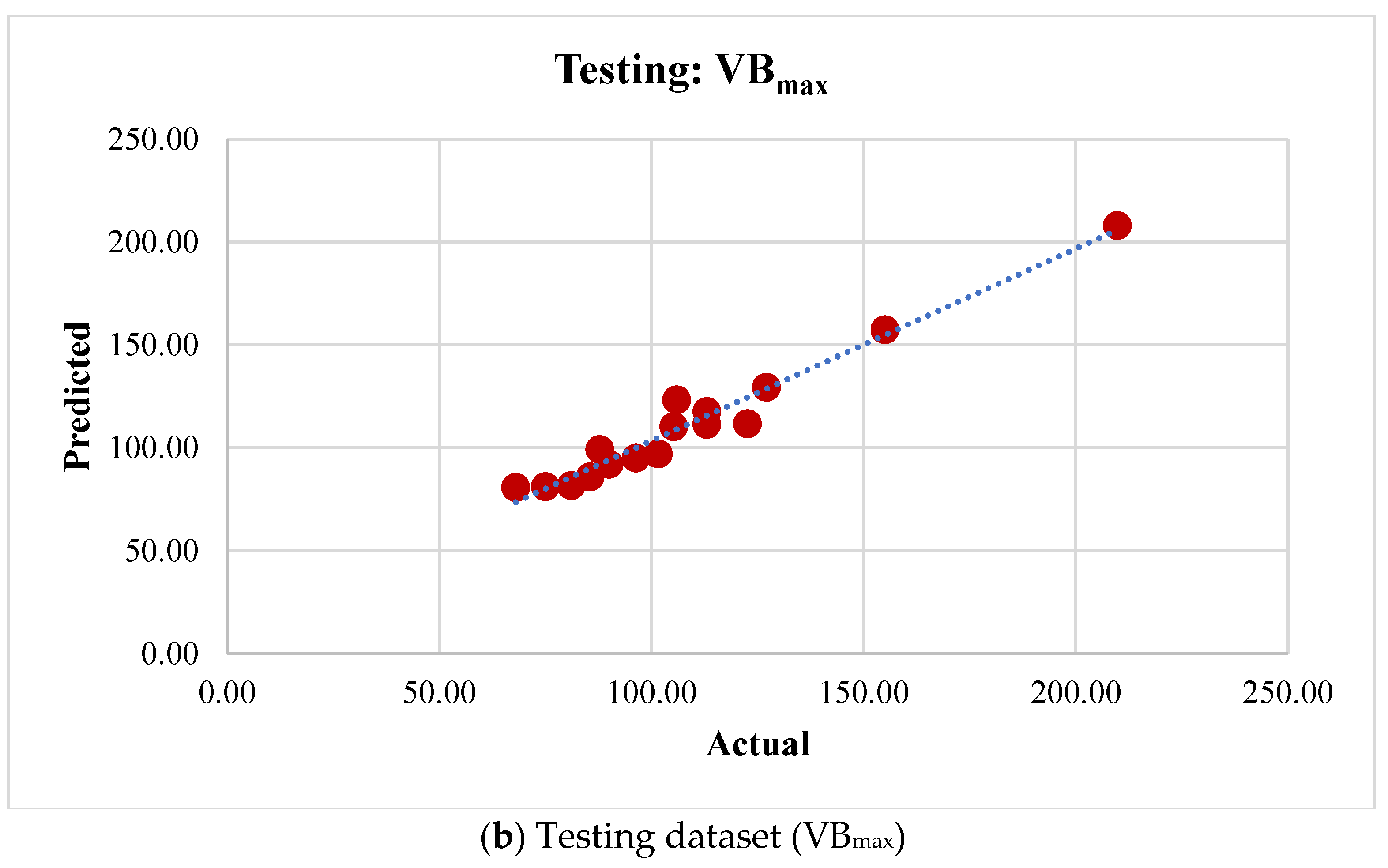
Additionally, the correlation between experimental and predicted R_max and VB_max values for training and test data is visualized through scatter plots in Figure 9 and Figure 10.

In both Figure 9 and Figure 10, the observations are densely aligned with the diagonal line of perfect correspondence, demonstrating a strong correspondence between model outputs and experimental observations for both R_max and VB_max. This visual consistency highlights the GPR models’ capability to effectively acquire the inherent patterns in the data.

These qualitative observations are supported by the quantitative performance metrics for the training and test sets summarized in Table 3 and Table 4. As shown in Table 3, for the training dataset, the models achieved exceptionally high coefficients of determination (R²) of 0.982 for R_max and 0.999 for VB_max, indicating that 98.2% and 99.9% of the variability in the actual values are captured by the respective models. The corresponding error metrics further confirm the high predictive accuracy and low deviation from actual values. For R_max, the error measures are SSE = 7.482, MSE = 0.115, RMSE = 0.339, MAE = 0.284, and MAPE = 3.962%, while for VB_max, SSE = 79.257, MSE = 1.219, RMSE = 1.104, MAE = 0.563, and MAPE = 0.613%.

As shown in Table 4, for the testing dataset, the models also demonstrated strong performance, with R² values of 0.964 for R_max and 0.953 for VB_max, reflecting excellent generalization capability. Although the error metrics are slightly higher than those of the training set, they remain within acceptable limits. For R_max, SSE = 6.605, MSE = 0.413, RMSE = 0.642, MAE = 0.474, and MAPE = 6.979%, whereas for VB_max, SSE = 844.933, MSE = 52.797, RMSE = 7.267, MAE = 5.343, and MAPE = 5.588%.

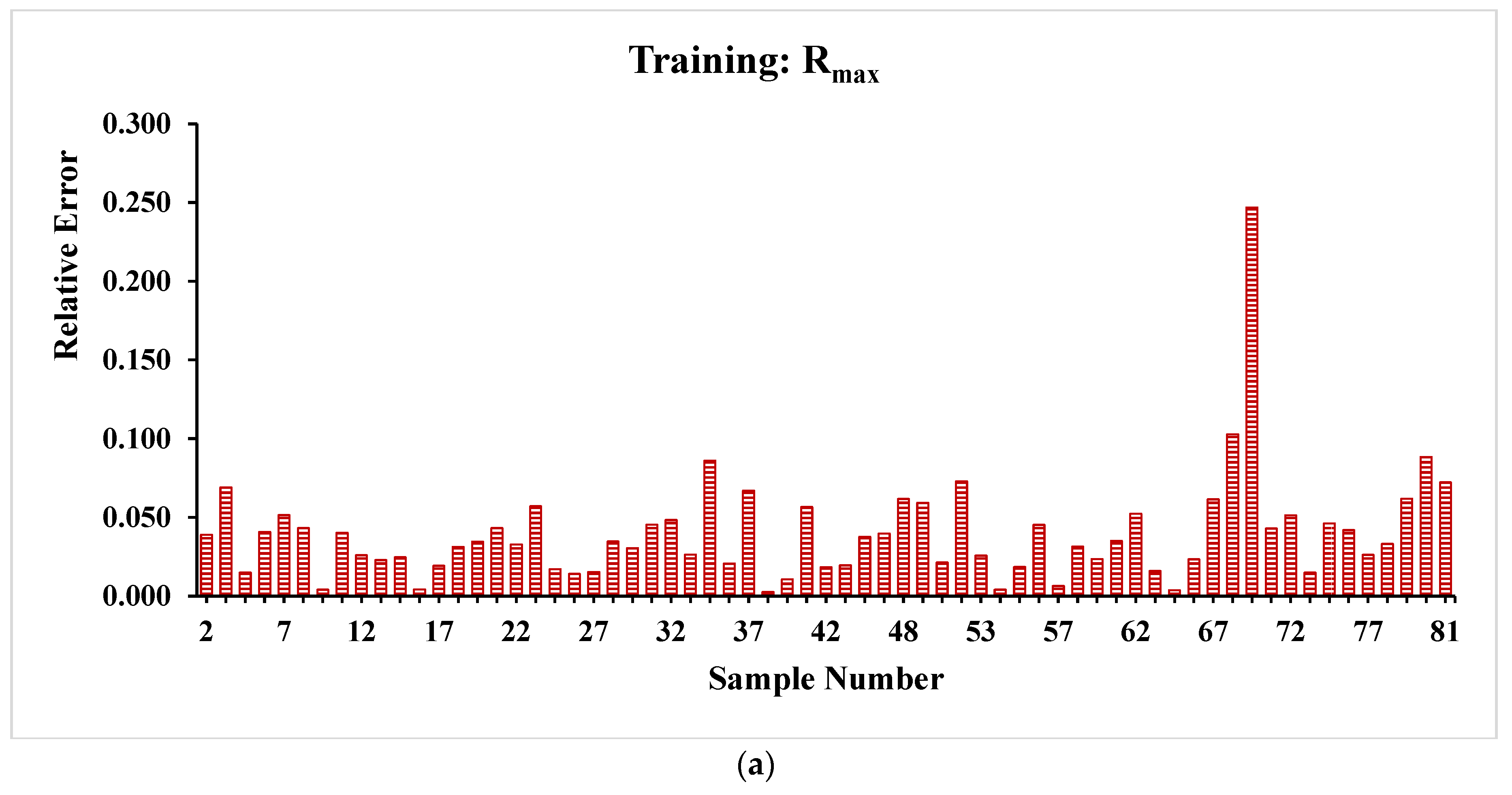
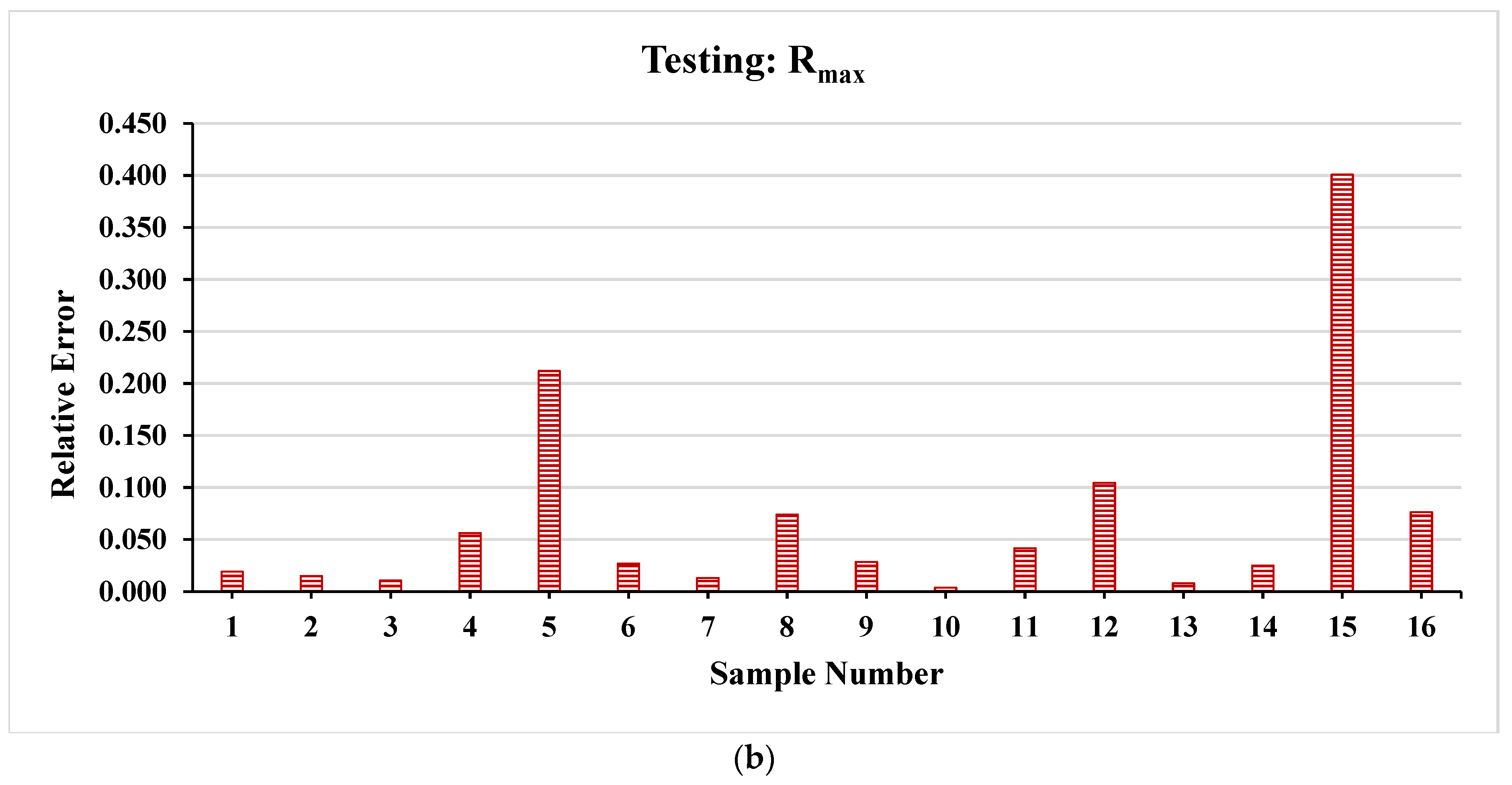
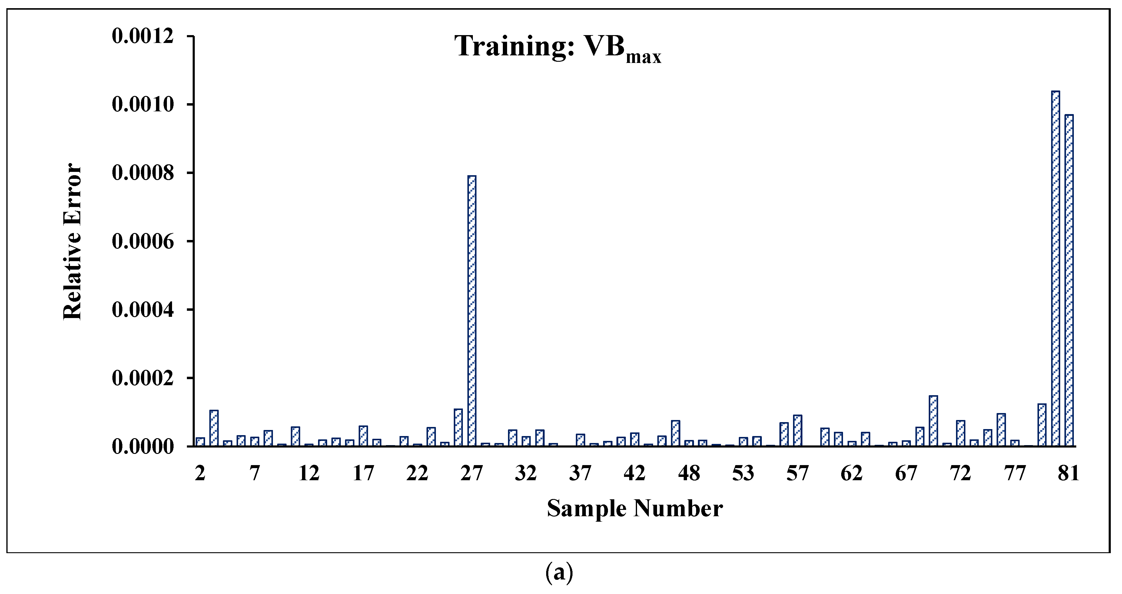
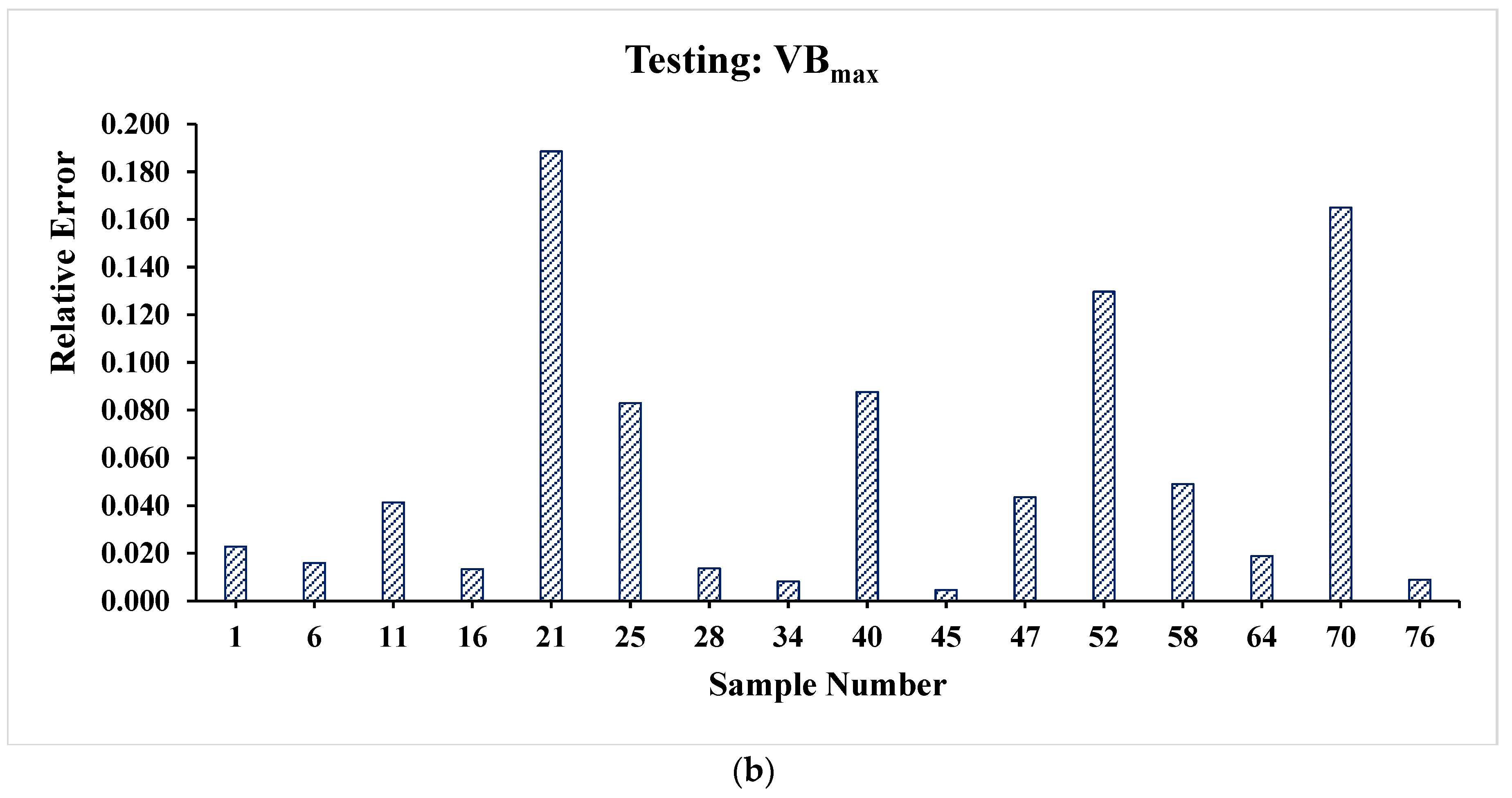
The relative errors for the training and test sets are illustrated in Figure 11 and Figure 12 for R_max and VB_max, respectively.

As shown in Figure 11 and Figure 12, the maximum relative error in the training dataset reaches approximately 0.25 and 0.001 for R_max and VB_max, respectively, while in the testing dataset it is slightly higher but remains within a limit of about 0.4 and 0.2 for R_max and VB_max, respectively. These results indicate that the model achieves low prediction error and demonstrates efficient and consistent performance in estimating both R_max and VB_max across the training and testing datasets.

These results confirm that the GPR model not only fits the training data well but also maintains robust and reliable predictive performance on new data, reinforcing its suitability for practical implementation in surface roughness prediction during machining processes.

4.3. Process Parameter Optimization

In the realm of machining process optimization, achieving minimal R_max and VB_max is a critical objective, as both directly influence the quality, functional performance, and performance of machined parts. The GPR machine learning model has demonstrated superior predictive accuracy. This superiority is evidenced by its effectiveness in capturing nonlinear interactions between process inputs and responses with high precision, as validated through rigorous cross-validation and statistical metrics, i.e., R², SSE, MSE, RMSE, MAE and MAPE.

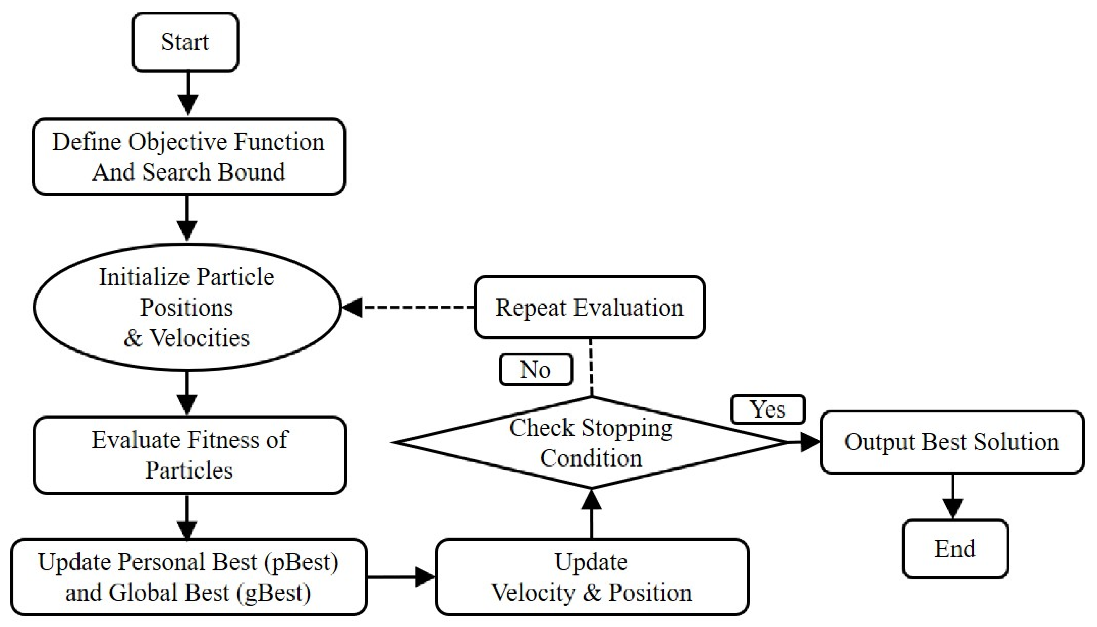
To further leverage the predictive capabilities of GPR, it was integrated with particle swarm optimization (PSO). As mentioned earlier, PSO is particularly well-suited for solving complex optimization problems due to its simplicity, efficiency, and ability to explore large search spaces effectively [3]. By integrating PSO with GPR, we aimed to identify the optimum machining parameters set that minimizes R_max and VB_max individually while adhering to operational constraints.

The PSO algorithm was implemented using the “particleswarm” function in MATLAB, configured to minimize the R_max and VB_max, as predicted by their trained GPR models. The GPR models act as surrogate objective functions within the PSO framework, guiding the swarm toward the parameter combination that yields optimal performance. The optimization variables include three categorical parameters (the cutting textures dimple, groove, and wave) encoded in one-hot format and three continuous parameters (cutting speed, feed rate, depth of cut), normalized via a standard score (z-score) scaling procedure. Constraints were imposed to ensure feasibility such as allowing only one active categorical variable and bounding the continuous variables within their normalized ranges.

A summary of the PSO configuration parameters used in both R_max and VB_max optimization is provided in

Table 5. Summary of GPR–PSO configuration.

Parameter	Value
Objective Function	A surrogate predictive model built upon GPR
Swarm Size	100 particles
Maximum Iterations	200 iterations
Bounds (Categorical)	Texture: One-hot (Dimple, Groove, Wave)
Bounds (Continuous)	Normalized using standard scaling: vc: [−1.48, 1.58], fr: [−1.38, 1.44], dc: [−1.40, 1.39]
Convergence Criterion	Relative change in objective value $<1\times {10}^{-6}$

. The optimization process terminated either upon reaching the maximum iteration count or when the relative change in the objective function value fell below a convergence threshold, ensuring both computational efficiency and convergence reliability.

The detailed outcomes of the PSO optimization, including both normalized and denormalized optimal parameter values, are presented in

Table 6. Optimal normalized and denormalized machining parameters predicted by the GPR–PSO models.

Parameter	Rmax		VBmax
	Optimal Value (Normalized)	Optimal Value (Denormalized)	Optimal Value (Normalized)	Optimal Value (Denormalized)
Texture type (One-Hot Encoding)	[0,1,0]	Groove	[0,0,1]	Wave
vc	−1.1685	76.35 m/min	0.4300	108.93 m/min
fr	−1.1468	0.064 mm/rev	−0.0192	0.1193 mm/rev
dc	−1.3255	0.355 mm	−1.3479	0.3481 mm
Predicted responses	-	2.554 μm	-	45.0390 μm

.

Table 7. Comparison between optimized and experimentally obtained lowest R_max and VB_max values.

Response	Condition	Texture Type	vc (m/min)	fr (mm/rev)	dc (mm)	Value	Improvement
Rmax	Optimal Level (GPR-PSO)	Groove	76.35	0.064	0.355	2.554	13.97%
	L27 Experimental (Corresponding to the Rmax lowest)	Groove	75.00	0.060	0.400	2.969
VBmax	Optimal Level (GPR-PSO)	Wave	108.93	0.1193	0.3481	45.039	30.70%
	L27 Experimental (Corresponding to the VBmax lowest)	Wave	125.00	0.1200	0.4000	65.000

presents a comparative analysis of the maximum roughness depth (R_max) and maximum flank wear (VB_max) obtained at the optimal cutting parameters predicted by the GPR–PSO models and the lowest values recorded during experimental trials.

As shown in Table 7, the R_max value predicted by the GPR–PSO model showed a 13.97% improvement compared to the lowest R_max observed in the L₂₇ experimental runs. Similarly, the VB_max value predicted by the framework demonstrated a 30.70% improvement over the minimum VB_max obtained experimentally. The optimal groove texture at the low feed and cutting speed can be attributed to its ability to accommodate cutting debris and reduce the effective contact area at the tool–workpiece interface, thereby improving surface roughness [34]. The wave texture at medium cutting speed provides a distributed textured contact that can reduce continuous sliding and adhesion, contributing to lower flank wear [25].

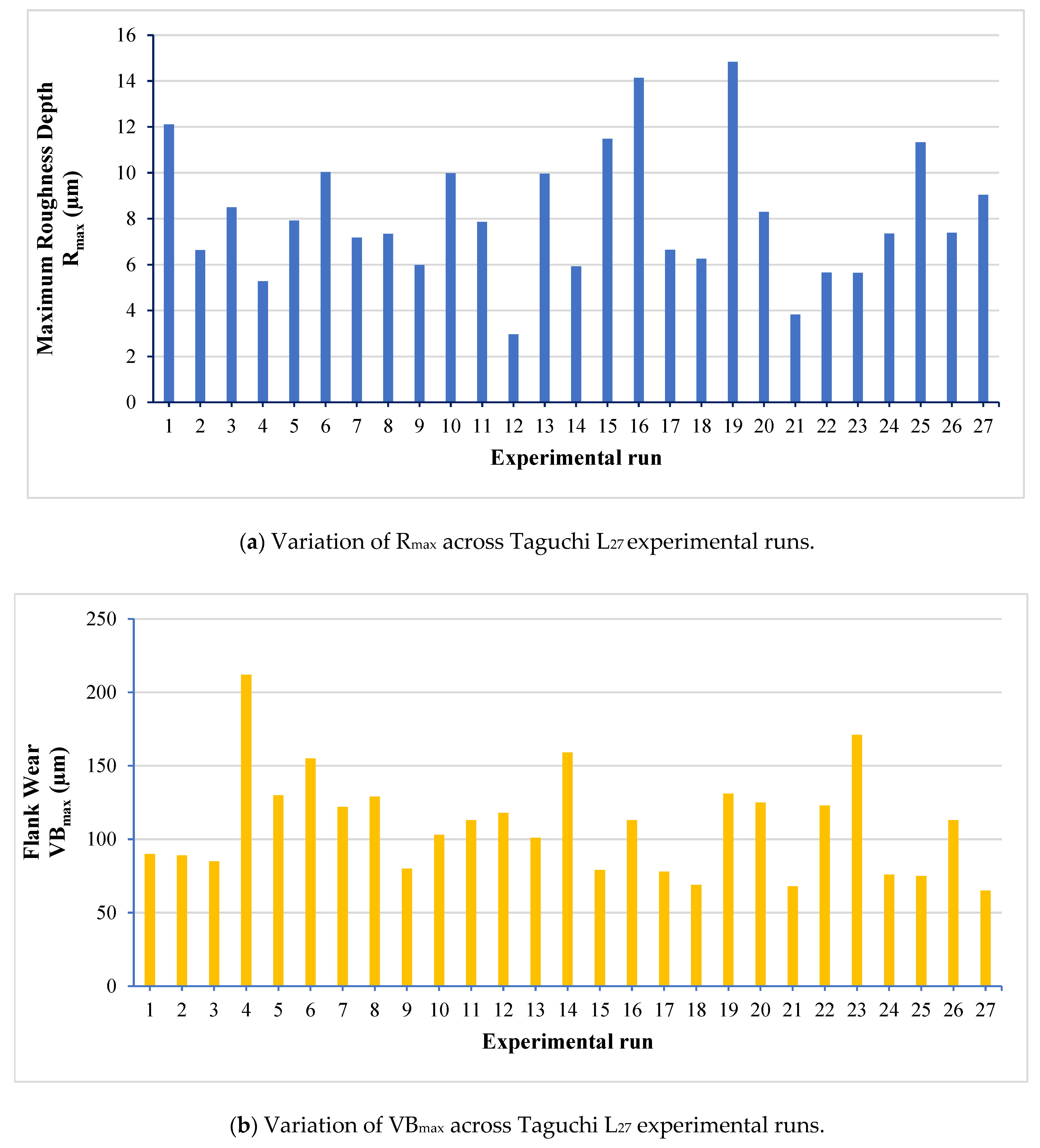
Specifically, the R_max was reduced from 2.969 μm (the minimum value obtained experimentally, as shown in Figure 2a, experimental run 12) to 2.554 μm under the optimal conditions identified by the GPR–PSO framework. In the case of VB_max, the value decreased from the experimentally observed minimum 65 μm (the minimum value obtained experimentally, as shown in Figure 2b, experimental run 27) to 45.039 μm under the optimized parameter settings. These reductions demonstrate the effectiveness of the GPR–PSO approach in determining machining parameters that minimize both maximum roughness depth and flank wear, thereby enhancing overall machining performance.

The successful identification of the optimal parameter sets, coupled with the robust convergence behavior of the PSO algorithm, highlights the efficacy of the GPR–PSO framework in addressing complex machining optimization problems. By leveraging the predictive accuracy of GPR and the global search efficiency of PSO, the framework achieves superior optimization performance while maintaining interpretability and adaptability across diverse operational scenarios. The results further confirm that the framework is highly effective in identifying optimal machining conditions when each performance metric is optimized individually.

However, it is important to note that the optimal parameter levels obtained for minimizing R_max and VB_max are not identical. This difference reflects the inherent trade-off between surface quality and tool wear during machining. While single-objective optimization provides valuable response-specific improvements, practical machining environments often require a balanced compromise between multiple performance criteria. Therefore, these findings motivate future work toward multi-objective optimization strategies capable of simultaneously considering R_max and VB_max, while also allowing for the inclusion of additional performance responses, to achieve globally efficient and application-oriented machining conditions.

5. Conclusions

This work introduces a systematic framework for optimizing machining performance using machine learning techniques, specifically GPR combined with PSO. The experimental investigations conducted on Super Duplex Stainless Steel (SDSS 2507) in dry turning with textured cutting inserts highlight the effectiveness of this integrated approach in precisely predicting and optimizing both maximum roughness depth (R_max) and maximum flank wear (VB_max). The developed GPR models exhibited remarkable predictive accuracy. For R_max, the training dataset achieved an R² value of 0.982 with SSE = 7.482, RMSE = 0.339, MAE = 0.284, and MAPE = 3.962%, while the testing dataset maintained strong predictive capability, with R² = 0.964, SSE = 6.605, RMSE = 0.642, MAE = 0.474, and MAPE = 6.979%. Similarly, the VB_max model demonstrated high reliability, with R² = 0.999 for training and 0.953 for testing, confirming the robustness and generalization ability of the framework. To mitigate data limitations and reduce overfitting risk, Gaussian data augmentation (GDA) was employed, enhancing dataset diversity and model stability. To further exploit the predictive strength of GPR, the models were integrated with PSO for parameter optimization. The optimization process successfully identified distinct optimal machining conditions for minimizing R_max and VB_max individually. The GPR–PSO framework achieved a 13.97% reduction in R_max and a 30.70% reduction in VB_max compared to the best measured results, confirming the practical effectiveness of the approach in improving machining performance.

The results highlight the strong capabilities of machine learning-driven optimization in precision machining. The proposed GPR–PSO framework enables intelligent parameter selection, leading to measurable improvements in surface quality and tool performance. Importantly, the difference between the optimal parameter settings for R_max and VB_max reveals the presence of inherent trade-offs in machining responses. This observation suggests that future work should be directed toward multi-objective optimization techniques capable of concurrently balancing several performance indicators, and potentially incorporating additional machining responses, to achieve globally efficient and industrially relevant operating conditions. In summary, this study demonstrates that data-driven optimization frameworks can significantly enhance machining efficiency and quality, providing a scalable pathway toward smarter and more sustainable manufacturing systems. The framework also offers practical potential as a decision-support approach for selecting machining conditions in industrial applications, where integration with process-monitoring and plant-specific machining data could facilitate its adaptation to real-world manufacturing operations.