Distributed Sensitivity-Conditioned Bilevel Optimization for Coordinated Control of Networked Microgrids

Abstract

This paper introduces a distributed sensitivity-conditioning approach for bilevel optimization in networked microgrids. The proposed method enhances the coordination between subsystems by embedding sensitivity-based predictive terms into the dynamic updates, thereby improving convergence stability without requiring strict time-scale separation. Unlike conventional singular perturbation techniques, the sensitivity-conditioning formulation enables faster and more robust convergence of the distributed dynamics under heterogeneous subsystem speeds. The approach is applied to a networked microgrid scenario where local agents perform decentralized optimization considering both internal generation and energy exchange with neighboring microgrids. Simulation results demonstrate that the proposed algorithm achieves efficient coordination, reduces convergence time, and maintains stability under diverse operating conditions. The results highlight the method’s potential as a scalable and computationally efficient alternative for real-time distributed energy management and bilevel control in power network applications.

1. Introduction

The increasing penetration of distributed energy resources and the progressive decentralization of electrical distribution systems have motivated the development of advanced coordination and control strategies for networked microgrids (NMGs) [1,2]. In these settings, local subsystems must continuously optimize their internal operation while simultaneously coordinating energy exchanges with neighboring microgrids. This naturally leads to hierarchical or bilevel decision-making structures in which local operational objectives interact with system-level coordination goals [3]. Achieving fast, stable, and scalable solutions to such optimization problems is essential for enabling real-time energy management, particularly under the variability and heterogeneity characteristic of modern microgrids [4,5].

A common approach to solving bilevel problems in distributed settings relies on singular perturbation arguments or time-scale separation: fast dynamics handle local optimization, while slower coordination dynamics ensure consistency across the network. The consensus problem has emerged as a compelling paradigm for orchestrating complex interactions in interconnected multi-agent systems [6]. Depending on the communication structure and control objectives, consensus can be approached from cooperative, distributed, or decentralized perspectives. By organizing agents in a decentralized manner, each one is in charge of making decisions individually [7]. This accommodates the inherent complexity of such systems, offering a structured framework to balance global objectives and local behaviors. One notable avenue to explore this concept from an optimization perspective is through the framework of bilevel optimization. Bilevel optimization extends traditional optimization paradigms by introducing two optimization layers: an upper-level optimization task that seeks to optimize a global objective, subject to constraints defined by lower-level optimization tasks [8,9]. This hierarchical formulation offers a natural means of integrating coordination and autonomy within complex systems.

In the context of multi-agent systems, the bilevel structure aligns well with the consensus methodology: the upper level represents a global coordination goal, while the lower levels correspond to the optimization of individual agent behaviors. Such an integration enables a unified framework for addressing coordination and consensus problems [10]. While effective under idealized assumptions, these methods encounter significant limitations in practice. Enforcing strict time-scale separation becomes increasingly difficult when subsystem dynamics operate at heterogeneous speeds, communication delays are present, or the system experiences rapid fluctuations in renewable generation and load. Moreover, singular perturbation-based algorithms often display degraded convergence properties or require conservative tuning to maintain stability, reducing their suitability for real-time operation [11]. To overcome these limitations, recent work has explored predictive or sensitivity-enhanced update rules that improve the behavior of distributed optimization algorithms without relying on idealized temporal structure [12]. However, most existing formulations either impose strong regularity assumptions, lack a systematic conditioning mechanism, or do not explicitly address the bilevel nature of microgrid coordination problems [13]. These gaps highlight the need for distributed methods that remain stable and efficient under heterogeneous subsystem speeds, reduce convergence time, and scale naturally with network size [14].

In the context of power systems, this hierarchical framework can be naturally extended to networks of networked microgrids, where each microgrid acts as an intelligent agent optimizing its local operational objectives—such as power balance or cost minimization while contributing to the overall network coordination goal [1,15]. At the upper level of this framework, the leader’s dynamics are formulated within a bilevel optimization structure, representing the global coordination layer of the networked microgrid system [10,16,17,18]. At this level, the objective is to minimize a global cost function, typically reflecting overall operational efficiency, economic dispatch, or power balance, defined as the aggregation of local microgrid costs while satisfying the corresponding global constraints. Complementing this, the lower level encompasses the individual optimization problems of each microgrid, where each entity seeks to optimize its own operational objectives, such as local generation–demand balance or energy trading, while accounting for its impact on the overall coordination goal [18,19].

To ensure effective coordination between the optimization levels, it is essential to characterize how agents are interconnected within the multi-agent network. These interconnections can be static or dynamic, homogeneous or heterogeneous, and may involve linear or nonlinear coupling depending on the communication topology and the nature of the agents’ interactions [20]. In the context of networked microgrids, such interconnections represent power-flow exchanges or information links that enable coordination among distributed generation units and local controllers [21,22]. In many practical settings, these interactions occur over different time-scales, where global coordination among microgrids evolves more slowly than the fast electrical and control dynamics within each unit [23]. Such multi-scale behavior complicates the relationship between local decision variables and the global coordination objective, often introducing sensitivity to parameter variations and dynamic conditions [24]. To systematically capture these effects, sensitivity analysis becomes a fundamental tool, enabling the quantification of how variations at the local or lower level influence the upper-level optimization outcomes [10,17,25]. The sensitivity-conditioning concept was proposed as an alternative to singular-perturbation/time-scale separation to accelerate nested dynamics while preserving stability [14]. Prior predictive-sensitivity work applied this idea to leader–follower dynamics and hierarchical decision problems [10,17]. Traditional microgrid coordination and distributed control approaches often rely on singular perturbation/time-scale separation for stability analysis, which can be restrictive under heterogeneous subsystem speeds. Finally, bilevel formulations for microgrid and distribution-grid interactions are an active area of research and provide a natural application domain for the proposed sensitivity-conditioning approach [26].

The main contribution of this paper is the introduction of a distributed sensitivity-conditioning approach for bilevel optimization in networked microgrids. The proposed work is methodological, supported by theoretical and application-driven advances. A distributed sensitivity-conditioned bilevel dynamic framework that relaxes restrictive time-scale separation assumptions inherent to classical hierarchical control is developed, while preserving convergence guarantees and enabling scalable real-time implementation in networked microgrids. The key idea is to embed sensitivity-based predictive terms into the dynamic updates of each subsystem, effectively conditioning the distributed dynamics to mitigate the impact of heterogeneity and reduce the need for strict time-scale separation. Unlike conventional singular perturbation techniques, the proposed formulation provides a principled means to accelerate convergence while preserving robustness in the presence of subsystem differences and real-world operational variability [17]. In the microgrid setting, these matrices capture how adjustments in local control actions, such as generation scheduling or voltage regulation, affect global synchronization metrics like frequency or power balance. The optimization levels interact dynamically, enabling the system to adapt to variations in both global objectives and local operating conditions. The proposed method ensures that the sensitivity matrices are computed efficiently, resulting in minimal additional computational burden. The effectiveness of the approach is demonstrated through simulations on a networked microgrid scenario. The results show that sensitivity-conditioning leads to faster convergence, improved stability characteristics, and efficient energy exchange coordination across diverse operating conditions. These properties make the proposed method a promising candidate for real-time distributed energy management, offering a scalable and computationally efficient alternative for bilevel control in emerging power network architectures.

Limitations of Existing Hierarchical and Bilevel Coordination Methods

Hierarchical and bilevel optimization frameworks have been widely investigated for the coordinated control and energy management of networked microgrids. Recent surveys highlight that most existing approaches can be broadly categorized into hierarchical control schemes, distributed optimization methods, and bilevel or Stackelberg-based formulations, each with distinct advantages and limitations [27,28]. A dominant class of bilevel control approaches relies on singular perturbation (SP) theory, where a strict time-scale separation between upper-level coordination and lower-level energy management is assumed. While analytically convenient, this assumption is difficult to enforce in practical microgrids, where pricing mechanisms, economic dispatch, and local EMS decisions often evolve on comparable time-scales. Violations of time-scale separation have been reported to cause slow transients and degraded performance, especially under fast demand fluctuations and renewable intermittency [28].

Alternative coordination strategies based on distributed optimization and ADMM have been proposed for economic dispatch and frequency regulation in microgrids. These methods typically require multiple inner iterations per control update and frequent communication among agents, leading to non-negligible latency and convergence-dependent runtime [29,30]. Such characteristics limit their applicability in real-time energy management scenarios with tight computational and communication constraints. Bilevel and Stackelberg game-based formulations have also been applied to microgrid operation, particularly for leader–follower pricing, demand response, and hybrid energy storage coordination [31,32]. While these methods effectively capture hierarchical decision-making structures, they often assume static lower-level optimal responses and embed the follower’s solution via Karush–Kuhn–Tucker (KKT) conditions or equilibrium reconstruction. This results in centralized implementations, increased numerical complexity, and limited robustness to modeling uncertainty and dynamic coupling effects. More recently, sensitivity-based leader–follower dynamics have been explored as a means to accelerate convergence by incorporating information on the followers’ response into the leader’s update law [17,18]. However, existing sensitivity-conditioned approaches are typically limited to static or centralized settings, rely on exact lower-level optimality, or lack rigorous convergence guarantees under distributed communication constraints and networked interactions.

The remainder of this paper is organized as follows. Section 2 introduces the Energy Management System (EMS) formulation for networked microgrids, describing the structure of the upper- and lower-level optimization problems. Section 3 presents the proposed sensitivity-conditioning framework for bilevel optimization and its analytical foundations, including assumptions, convergence properties, and algorithmic formulation. Section 4 validates the proposed dynamics using a benchmark classification problem and analyzes the convergence improvement introduced by the sensitivity-conditioning term. Finally, Section 5 summarizes the main findings and outlines future research directions.

Notation. The set of real numbers is denoted as $\mathbb{R}$. $\mathbf{X}$ and x denote matrices and vectors, respectively. We write ${\mathbf{X}}^{\top }$, $x^{\top }$, $f{(·)}^{\top }$ for the transpose of a matrix, a vector, or a function, respectively. The optimal values in the optimization problems are denoted as $x^{\ast },X^{\ast }$. variables with overlines and underlines denote upper and lower limits, respectively (e.g., ${\overline{p}}_i$ and ${\underline{p}}_i$ represent the maximum and minimum power of unit i). In graph theory, the Laplacian matrix of a graph is defined as $\mathbf{L}=\mathbf{D}-\mathbf{A}$, where $\mathbf{D}$ is the degree matrix, and $\mathbf{A}$ is the adjacency matrix. Based on the structure of $\mathbf{L}$, at least one of its eigenvalues is zero and the rest have non-negative real parts. A digraph G is weight-balanced if and only if ${\mathbf{1}}_N^{\top }\mathbf{L}=\mathbf{0}$.

2. Energy Management System for Networked Microgrids

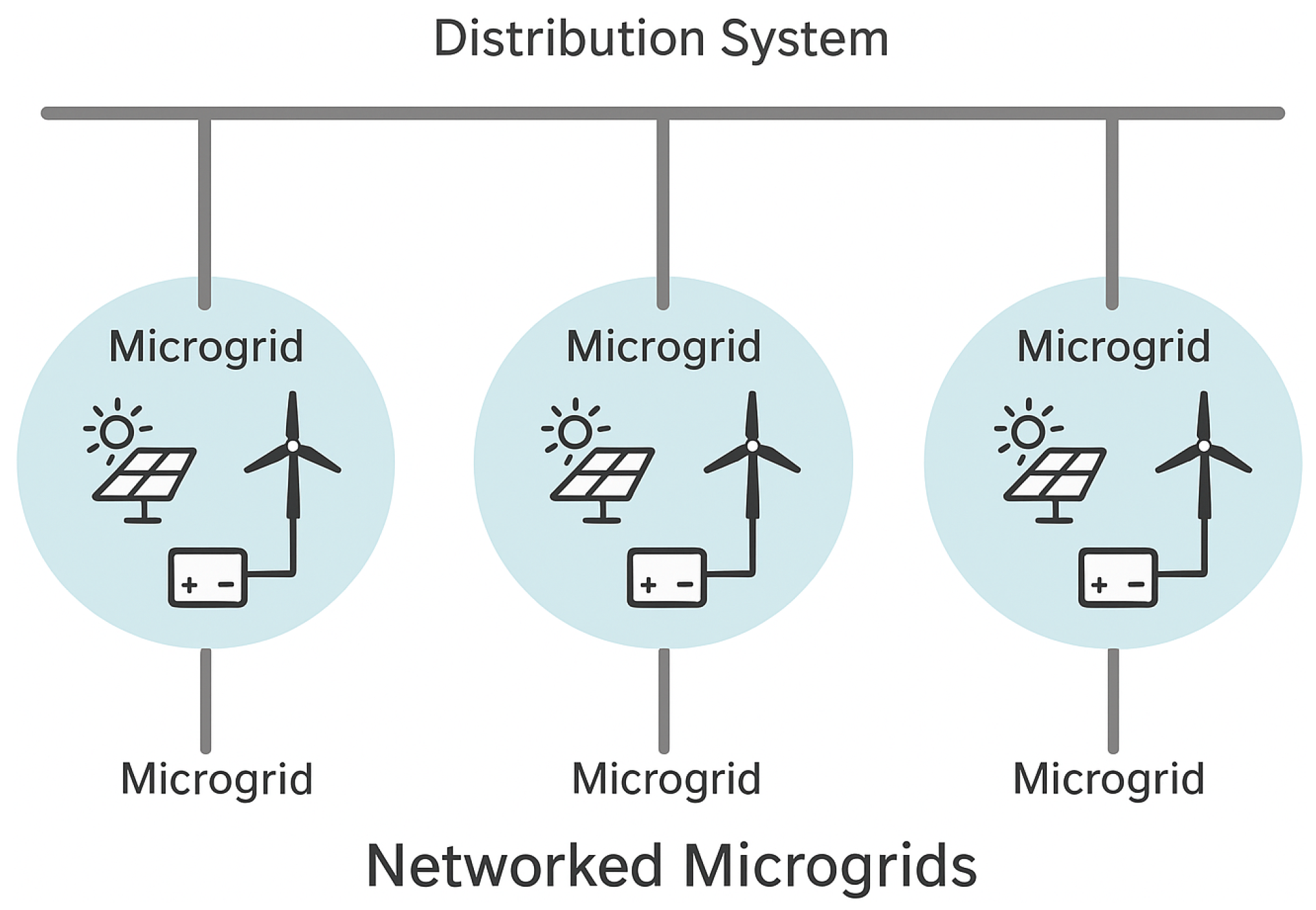
A microgrid (MG) is a localized cluster of distributed energy resources, storage units, and controllable loads operating under a coordinated control scheme, capable of functioning both in grid-connected and islanded modes [33]. When several MGs interact and exchange energy or information through a common distribution system (DS), they form a networked microgrid (NMG) [1]. This interaction enhances overall reliability, efficiency, and economic performance by enabling cooperative energy sharing among NMGs. As illustrated in Figure 1, the NMG architecture extends beyond individual MGs to include the DS, forming a hierarchical network where local and global energy management layers coexist. Similar to isolated MGs, the Energy Management System (EMS) arises as a central component in NMG operations. This energy management considers the individual EMS of every MG involved and the transactions between them. This section shows some features, notation, and the EMS formulation for NMG systems starting from the EMS problem of individual MGs.

2.1. Global Features

One of the essential features of NMG systems is the capability to exchange power among neighboring subsystems. These exchanges occur through the Points of Common Coupling (PCCs), which define the physical interconnections between microgrids and enable flexible network configurations. Through these PCCs, the NMG topology can dynamically adapt, allowing each MG to operate either in islanded mode or in a connected configuration depending on operational conditions and coordination objective.

Since the NMG system comprises MGs (nodes) and PCCs (links), we use graph theory to represent it as $\mathcal{D}=(\mathcal{N},\mathcal{E})$, where $\mathcal{N}=\{1,\dots ,N\}$ is the set of involved MGs and $\mathcal{E}\subseteq \mathcal{N}\times \mathcal{N}$ is the set of links between neighboring MGs. Moreover, we use subindexes i and j to denote members in $\mathcal{N}$.

2.2. Single Microgrid EMS

To better understand the optimization problem within each subsystem, this subsection describes the EMS formulation for a single MG before extending it to the NMG context. Internally, each MG is a usual electrical system comprising distributed generators and local consumption. Distributed generators are commonly based on wind turbines, photovoltaic plants, and dispatchable resources such as micro-turbine generators. In the same way, MGs could suffer from energy shortages, system failures, and high energy prices. Through boundary buses and PCCs, interaction with similar systems solves most of these problems by exchanging power capacity. The EMS problem of single MGs can be formulated as a constrained optimization problem, defined as

$$\underset{u_i\left(t\right)}{\min }{J}_i={\int }_{t_0}^{t_f}\left(C_i^{\mathrm{op}}\left(p_i^{\mathrm{DG}}\left(t\right),p_i^{\mathrm{ESS}}\left(t\right),{\ell }_i\left(t\right)\right)+C_i^{\mathrm{tr}}\left(p_i^{\mathrm{PCC}}\left(t\right)\right)\right)dt$$

(1)

$$\begin{array}{cc}\hfill \mathrm{s}.\mathrm{t}.& p_i^{\mathrm{DG}}\left(t\right)+p_i^{\mathrm{ESS}}\left(t\right)+p_i^{\mathrm{PCC}}\left(t\right)={\ell }_i\left(t\right),\hfill \end{array}$$

(2)

$$\begin{array}{cc}\hfill & 0\le p_i^{\mathrm{DG}}\left(t\right)\le {\overline{p}}_i^{\mathrm{DG}},\hfill \end{array}$$

(3)

$$\begin{array}{cc}\hfill & {\dot{e}}_i\left(t\right)={\eta }_c{p}_i^{\mathrm{ch}}\left(t\right)-{\displaystyle \frac{1}{{\eta }_d}}{p}_i^{\mathrm{dis}}\left(t\right),e_i^{\min }\le e_i\left(t\right)\le e_i^{\max },\hfill \end{array}$$

(4)

$$\begin{array}{cc}\hfill & p_i^{\mathrm{ESS}}\left(t\right)=p_i^{\mathrm{dis}}\left(t\right)-p_i^{\mathrm{ch}}\left(t\right),0\le p_i^{\mathrm{ch}}\left(t\right)\le {\overline{p}}_i^{\mathrm{ch}},0\le p_i^{\mathrm{dis}}\left(t\right)\le {\overline{p}}_i^{\mathrm{dis}},\hfill \end{array}$$

(5)

$$\begin{array}{cc}\hfill & -{\overline{p}}_i^{\mathrm{PCC}}{\sigma }_i\left(t\right)\le p_i^{\mathrm{PCC}}\left(t\right)\le {\overline{p}}_i^{\mathrm{PCC}}{\sigma }_i\left(t\right),{\sigma }_i\left(t\right)\in \{0,1\},\hfill \end{array}$$

(6)

$$\begin{array}{cc}\hfill & u_i\left(t\right)=\left\{p_i^{\mathrm{DG}}\left(t\right),p_i^{\mathrm{ch}}\left(t\right),p_i^{\mathrm{dis}}\left(t\right),p_i^{\mathrm{PCC}}\left(t\right),{\sigma }_i\left(t\right)\right\}.\hfill \end{array}$$

(7)

In the single microgrid optimization problem, $J_i$ denotes the total cost incurred by the i-th MG over the time horizon $[t_0,t_f]$, which includes both internal operational costs and costs associated with energy transactions through the PCC. The decision variables are grouped in $u_i\left(t\right)$, which contains the controllable power setpoints of the distributed generators $p_i^{\mathrm{DG}}\left(t\right)$, the charging and discharging powers of the energy storage system $p_i^{\mathrm{ch}}\left(t\right)$ and $p_i^{\mathrm{dis}}\left(t\right)$, the exchanged power through the point of common coupling $p_i^{\mathrm{PCC}}\left(t\right)$, and the binary variable ${\sigma }_i\left(t\right)$ indicating the connection status of the MG. The power balance constraint (2) enforces the instantaneous equality between generation, storage, exchange, and demand ${\ell }_i\left(t\right)$. Equation (3) imposes upper and lower bounds on the generation capacity of the DG units. The state-of-charge dynamics of the storage system are expressed in (4), where $e_i\left(t\right)$ represents the stored energy and ${\eta }_c$ and ${\eta }_d$ denote the charging and discharging efficiencies, respectively. The constraint (5) limits the charging and discharging rates to their corresponding maximum values, ensuring that the ESS operates within its technical limits. Finally, constraint (6) restricts the power exchanged through the PCC to a maximum allowable capacity ${\overline{p}}_i^{\mathrm{PCC}}$, which is active only when the MG is connected to the network (${\sigma }_i=1$).

This formulation provides the local energy management framework for a single MG, capturing its internal operation, storage dynamics, and interaction with the distribution network through the PCC. Although each MG is capable of operating autonomously, its performance can be significantly improved through coordinated operation with neighboring MGs, especially under conditions of generation scarcity, demand fluctuations, or varying electricity prices [1]. Consequently, the extension of this formulation to a networked configuration enables the joint optimization of multiple MGs, forming the basis for the Energy Management System of NMGs, which is developed in the following subsection.

2.3. Networked Microgrid Energy Management System

Considering that the NMG system comprises a set of MGs $\mathcal{D}$, where each MG is modeled by the local EMS problem defined in (1), the objective function of the NMG can be expressed as the summation of the individual costs of all MGs. In this way, the global optimization problem aims to minimize the total operating cost of the network while respecting the local constraints of each MG. Consequently, the constraints derived from the single MG formulation collectively form the global constraint set of the NMG EMS, which governs energy trading and coordination among MGs in the retail market.

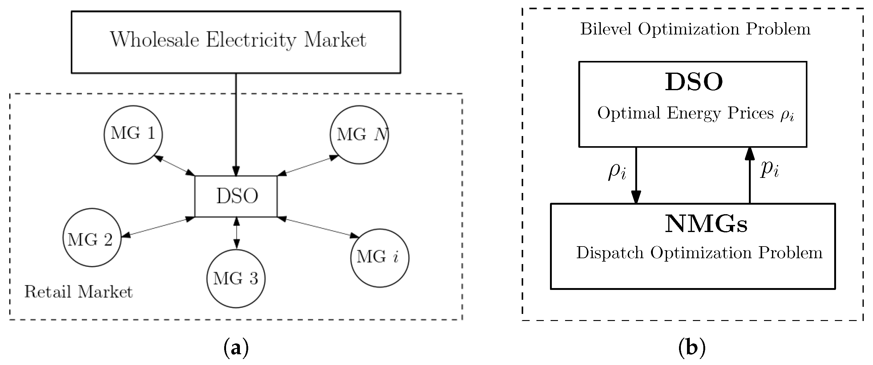
Initially, the leader, represented by the distribution system operator (DSO), establishes the marginal price ${\rho }_i$ for each MG $i\in \mathcal{D}$ according to the network operating conditions and market signals. Each MG then receives this price signal and solves its local EMS problem defined in (1), determining its optimal generation dispatch $p_i^{\mathrm{DG}}\left(t\right)$ and power exchange $p_i^{\mathrm{PCC}}\left(t\right)$ to satisfy the local demand ${\ell }_i\left(t\right)$ and contribute to the overall distribution system power balance $P^{\mathrm{DS}}$. Figure 2a illustrates the hierarchical interaction between the wholesale electricity market, the DSO, and the individual MGs participating in the retail market. The DSO acts as an intermediary entity, coordinating energy exchange and price signals between higher-level markets and distributed energy resources.

The coordination mechanism between the DSO and the microgrids can be modeled as a bilevel optimization problem, as depicted in Figure 2b. In this structure, the upper level corresponds to the DSO, which determines the optimal marginal prices ${\rho }_i$, while the lower level comprises the MGs that individually solve their EMS problems to determine their optimal generation and exchange power. This hierarchical relationship enables the integration of distributed decision-making within a unified optimization framework.

We propose a bilevel optimization problem to solve the energy management of the NMG system. At the upper level, the objective is to maximize the welfare function $W(\mathit{\rho },\mathbf{p})$, while at the lower level the aim is to minimize the cost of microgrid generation $C(\mathit{\rho },\mathbf{p})$. Here, $\mathit{\rho }={[{\rho }_1,{\rho }_2,\dots ,{\rho }_{\left|\mathcal{D}\right|}]}^{\top }$ denotes the vector of marginal prices determined by the DSO for each MG, and $\mathbf{p}={[p_1^{\mathrm{DG}},p_2^{\mathrm{DG}},\dots ,p_{\left|\mathcal{D}\right|}^{\mathrm{DG}}]}^{\top }$ represents the vector of generation outputs or exchanged power from the individual MGs. The bilevel optimization problem can be stated as

$$\begin{array}{cc}\hfill \underset{\rho }{\max }W(\mathit{\rho },{\mathbf{p}}^{\ast }\left(\mathit{\rho }\right))& ={\displaystyle \frac{1}{N}}\sum _{i=1}^N\left({\rho }_i{p}_i^{\mathrm{PCC}\ast }\left({\rho }_i\right)-e_i{\rho }_i{p}_i^{\mathrm{PCC}\ast }\left({\rho }_i\right)\right),\hfill \\ \hfill \mathrm{s}.\mathrm{t}.& {\mathbf{p}}^{\ast }\left(\mathit{\rho }\right)\in \arg \underset{\mathbf{p}}{\min }C(\mathit{\rho },\mathbf{p})={\displaystyle \frac{1}{N}}\sum _{i=1}^N\left(c_i{\left(p_i^{\mathrm{DG}}\right)}^2+b_i{p}_i^{\mathrm{DG}}+a_i-{\rho }_i{p}_i^{\mathrm{DG}}\right),\hfill \\ \hfill & \sum _{i=1}^N{p}_i^{\mathrm{PCC}}=P^D+P^{DS},\hfill \\ \hfill & {\underline{p}}_i^{\mathrm{DG}}\le p_i^{\mathrm{DG}}\le {\overline{p}}_i^{\mathrm{DG}},\forall i\in \mathcal{D}.\hfill \end{array}$$

(8)

In this formulation, the optimal responses of the lower-level problems, $p_i^{\mathrm{PCC}\ast }\left({\rho }_i\right)$, are then used by the upper-level DSO to maximize the system welfare $W(\mathit{\rho },\mathbf{p})$. The parameters $a_i$, $b_i$, and $c_i$ are cost coefficients associated with the quadratic generation cost function of MG i, representing fixed, linear, and quadratic terms, respectively.

To describe the continuous-time evolution toward the equilibrium defined by the bilevel optimization problem (8), the dynamic behavior of each MG can be modeled as

$${\dot{p}}_i^{\mathrm{PCC}}=-\left(2c_i{p}_i^{\mathrm{PCC}}+b_i-{\rho }_i+\nu \right),\mathrm{with}\sum _{i=1}^N{\dot{p}}_i^{\mathrm{PCC}}=0.$$

(9)

Here, $\nu$ represents a global dynamic Lagrange multiplier that enforces the power balance among all MGs, as defined in (8). It differs from the local multipliers ${\rho }_i$ associated with the internal constraints of each MG, since $\nu$ is a shared variable coordinating the interaction among subsystems through the distribution network:

$$\sum _{i=1}^N{p}_i^{\mathrm{PCC}}\left(t\right)=P^D+P^{DS},\forall t\ge 0.$$

(10)

The DSO updates the price according to

$${\dot{\rho }}_i=p_i^{\mathrm{PCC}}(1-{ϵ}_i),$$

(11)

with ${\mathbf{p}}^{\mathrm{PCC}}={[p_1^{\mathrm{PCC}},\dots ,p_N^{\mathrm{PCC}}]}^{\top }$ and, $\mathbf{ffl}={[{ϵ}_1,\dots ,{ϵ}_N]}^{\top },$ with the coupled dynamics written as

$$\left[\begin{array}{c}{\dot{\mathbf{p}}}^{\mathrm{PCC}}\\ \dot{\mathit{\rho }}\end{array}\right]=\left[\begin{array}{c}-{\nabla }_{{\mathbf{p}}^{\mathrm{PCC}}}\mathcal{L}({\mathbf{p}}^{\mathrm{PCC}},\mathit{\rho })+\nu \mathbf{1}\\ {\mathbf{p}}^{\mathrm{PCC}}\circ (1-\mathbf{ffl})\end{array}\right],$$

(12)

where

$$\mathcal{L}({\mathbf{p}}^{\mathrm{PCC}},\mathbf{\rho })=\sum _{i=1}^N\left(c_i{\left(p_i^{\mathrm{PCC}}\right)}^2+b_i{p}_i^{\mathrm{PCC}}+a_i-{\rho }_i{p}_i^{\mathrm{PCC}}\right).$$

The coupled dynamic model presented above captures the continuous-time interaction between the DSO and the MGs within the NMG system. Through these dynamics, the MGs iteratively adjust their exchanged power $p_i^{\mathrm{PCC}}$ in response to the price signals ${\rho }_i$, while the DSO updates these prices according to the aggregated network behavior. The term $\nu$ acts as a global coupling variable that enforces power balance, ensuring coordinated evolution toward the optimal equilibrium defined by the bilevel optimization framework. The parameter ${ϵ}_i$ represents the sensitivity of each MG to price variations, influencing the rate of adaptation of the price dynamics. This reduced formulation intentionally focuses on the coordination and economic dispatch layer of the EMS, abstracting faster electrical and device-level dynamics that are typically handled by local controllers and are not critical for analyzing price-based inter-microgrid coordination. As such, it captures the essential EMS behavior relevant to bilevel coordination while remaining analytically tractable, which naturally motivates the sensitivity-based approach developed in the following section.

3. A Sensitivity-Conditioning for Bilevel Optimization

In this section, we show how decentralized interconnected systems with two-time-scale decentralized interconnected systems can be reformulated into a single-time-scale framework by means of a predictive-sensitivity matrix in continuous time. Initially, we introduce the concept of the sensitivity matrix that relates the dynamics of the systems to a bilevel optimization problem.

Building upon the bilevel formulation introduced in the previous section, we now express the general structure of leader–follower optimization problems in a compact form. This abstraction allows extending the NMG coordination problem to a broader class of decentralized multi-agent systems. Traditionally, we define a set of leader agents as the upper-level problem, and the followers’ optimization problem is referred to as the lower-level problem. Each level has its own set of variables, constraints, and objective functions, as defined by

$$\begin{array}{cc}\hfill \underset{x\in {\mathbb{R}}^p}{\min }& F(x,y^{\ast }\left(x\right))={\displaystyle \frac{1}{N}}\sum _{i=1}^N{f}_i(x,y^{\ast }\left(x\right))\hfill \end{array}$$

(13)

$$\begin{array}{cc}\hfill \mathrm{s}.\mathrm{t}.& y^{\ast }\left(x\right)\in \arg \underset{y\in {\mathbb{R}}^q}{\min }G(x,y)={\displaystyle \frac{1}{N}}\sum _{i=1}^N{g}_i(x,y),\hfill \end{array}$$

(14)

where $x\in {\mathbb{R}}^p$ is the upper-level variable, and $y\in {\mathbb{R}}^q$ is the lower-level variable, $F(x,y)$ is the objective function of the leader agents, and $G(x,y)$ is the objective function of the followers. We can assume that each leader has an objective function $f_i(x,y)$ with $i=1,2,\dots ,N$, and each follower $g_i(x,y)$, where N is the number of agents. The predictive-sensitivity matrix captures how changes in the leader’s variables x affect the followers’ responses $y^{\ast }\left(x\right)$, thus linking the upper- and lower-level problems in continuous time. The following assumptions will be used, which are standard in bilevel optimization and decentralized optimization literature [34].

Assumption 1.

$F(x,y)$ is assumed twice continuously differentiable, and $G(x,y)$ is three times continuously differentiable, both with Lipschitz continuous partial derivatives.

Assumption 2.

Function $g_i$ is assumed μ-strongly convex in y for all i.

In microgrid applications, generation and exchange costs are commonly modeled using quadratic or piecewise-quadratic functions, reflecting fuel costs, wear-and-tear, and efficiency losses. When convex operational constraints are enforced (generation limits, storage bounds), the resulting EMS problems are strongly convex in most operating regions.

Assumption 3.

For every x, the lower-level problem admits at least one solution $y^{\ast }\left(x\right)$, and the Hessian ${\nabla }_{yy}^{2}G(x,y^{\ast }\left(x\right))$ is nonsingular.

For differentiable EMS cost functions with strictly convex structure, sensitivity matrices naturally arise from the implicit function theorem and can be computed analytically or numerically with low computational effort. In real-time microgrid operation, these sensitivities can be updated either analytically (for quadratic models), or via local linearization around the current operating point. Thus, this assumption is practically reasonable for EMS models deployed in real-time controllers. For differentiable EMS cost functions with strictly convex structure, sensitivity matrices naturally arise from the implicit function theorem and can be computed analytically or numerically with low computational effort.

Assumption 4.

The communication graph among agents is strongly connected and weight-balanced. Moreover, it contains a spanning tree with the leader as the root node.

In NMGs, communication networks are typically designed to ensure at least weak connectivity, often via supervisory controllers or distribution system operators (DSOs). Weight-balanced or approximately balanced graphs naturally arise in peer-to-peer communication protocols and consensus-based coordination mechanisms used in energy management. Temporary communication failures, packet losses, or topology changes may violate this assumption. While the current analysis ensures convergence under fixed or slowly switching connected topologies, abrupt or prolonged disconnections may degrade performance. Nevertheless, the distributed nature of the algorithm allows microgrids to continue operating locally, preserving safety even when global optimality is temporarily lost.

Under Assumption 1, the invertibility assumption defines the sensitivity of $y^{\ast }$. Then, the implicit-function theorem [35] guarantees the local existence of the map $y^{\ast }\left(x\right)$, and gives an expression for its derivative as

$${\nabla }_x{y}^{\ast }\left(x\right)=-{\left({\nabla }_{yy}^{2}G(x,y^{\ast }\left(x\right))\right)}^{-1}{\nabla }_{yx}^{2}G(x,y^{\ast }\left(x\right))=-{\displaystyle \frac{1}{N}}\sum _{i=0}^N{\left({\nabla }_{yy}^2{g}_i(x,y^{\ast }\left(x\right))\right)}^{-1}{\nabla }_{yx}^2{g}_i(x,y^{\ast }\left(x\right)).$$

(15)

For a given x, Assumption 1 ensures that the lower-level problem in (8) admits at most one optimal solution, denoted by $y^{\ast }\left(x\right)$. The mapping $y^{\ast }\left(x\right)$ allows for defining a reduced objective function $f^r\left(x\right):=F(x,y^{\ast }\left(x\right))$, whose gradient leads to the definition of the total derivative:

$$D_{x}F(x,y^{\ast }\left(x\right)):={\nabla }_x{f}^r\left(x\right)={\nabla }_{x}F(x,y^{\ast }\left(x\right))+{\nabla }_x{y}^{\ast }{\left(x\right)}^{\top }{\nabla }_{y}F(x,y^{\ast }\left(x\right))={\displaystyle \frac{1}{N}}\sum _{i=1}^N{\nabla }_x{f}_i(x,y^{\ast }\left(x\right)),$$

(16)

for points where $y=y^{\ast }\left(x\right)$. Under Assumptions 1–3, the Hessian ${\nabla }_{yy}^{2}G(x,y)$ is invertible for y in a neighborhood of $y^{\ast }\left(x\right)$. Since it is generally not possible to compute ${\nabla }_x{y}^{\ast }\left(x\right)$ directly, ${\nabla }_x{f}^r\left(x\right)$ can be approximated using the sensitivity matrix, defined as

$$\begin{array}{cc}\hfill D_{x}F(x,y)& ={\nabla }_{x}F(x,y)+S_x^y{(x,y)}^{\top }{\nabla }_{y}F(x,y),\hfill \end{array}$$

(17)

$$\begin{array}{cc}\hfill S_x^y(x,y)& =-{\nabla }_{yy}^{2}G{(x,y)}^{-1}{\nabla }_{yx}^{2}G(x,y),\hfill \end{array}$$

(18)

where $S_x^y(x,y)$ quantifies how variations in the upper-level variables x affect the lower-level responses y.

Geometrically, it represents the local Jacobian of the optimal-response manifold $y^{\ast }\left(x\right)$, describing how the follower equilibrium deforms as the leader dynamics evolve. From a dynamical perspective, the inclusion of $S_y^x$ introduces a predictive feed-forward correction that anticipates the impact of leader updates on follower equilibria, thereby reducing inter-level lag and improving damping. In the microgrid context, this matrix admits a physical interpretation as a price–response sensitivity, quantifying how local power exchange decisions react to marginal price variations imposed by the DSO.

From a numerical standpoint, the sensitivity matrix is computed by solving the linear system ${\nabla }_{yy}^{2}G(x,y)S=-{\nabla }_{yx}^{2}G(x,y)$, rather than explicitly forming the inverse of ${\nabla }_{yy}^{2}G(x,y)$, which improves numerical robustness.

In the economic dispatch formulation considered in this work, the lower-level objective is quadratic and separable across microgrids, which implies that ${\nabla }_{yy}^{2}G(x,y)$ is diagonal and positive definite. As a result, the sensitivity matrix $S_y^x$ admits a closed-form expression that can be computed locally by each agent, significantly reducing the computational burden compared to general bilevel optimization settings and mitigating potential conditioning issues.

These quantities satisfy the following consistency conditions:

$$\begin{array}{cc}\hfill D_{x}F(x,y){|}_{(x,y^{\ast }\left(x\right))}& ={\nabla }_x{f}^r\left(x\right),\hfill \end{array}$$

(19)

$$\begin{array}{cc}\hfill S_x^y(x,y){|}_{(x,y^{\ast }\left(x\right))}& ={\nabla }_x{y}^{\ast }\left(x\right).\hfill \end{array}$$

(20)

To guarantee that a solution for the optimization problem (14) exists, we propose the following definition.

Definition 1.

A pair $(x^{\ast },y^{\ast })$ is said to be a local solution to the bilevel optimization problem (14) if

1. 

$y^{\ast }$ is a local minimizer of the lower-level problem $G(x^{\ast },y)$;

2. 

there exists a neighborhood $\mathcal{N}$ of $x^{\ast }$ such that

$$F(x^{\ast },y^{\ast })\le F(x,y^{\ast }\left(x\right))\forall x\in \mathcal{N},$$

where $y^{\ast }\left(x\right)$ denotes a local solution of the lower-level problem associated with x.

The sensitivity-conditioned bilevel optimization framework considered in this work is inspired by the predictive sensitivity-based interconnection originally proposed in [14]. While that framework addresses generic bilevel optimization problems, the present work specializes the approach to the economic dispatch problem in networked microgrids. In particular, the quadratic structure of the lower-level cost functions and the power balance constraints enable an explicit and decentralized construction of the sensitivity matrix, as well as a physically interpretable coupling with consensus-based coordination dynamics.

The dynamics to obtain the solution of the system can be defined based on [36] as a dynamic consensus problem of the form

$$\begin{array}{cc}\hfill {\dot{x}}_i& =-D_x{f}_i(x_i,y_i)-\beta \sum _{j=1}^N{a}_{ij}(x_i-x_j)-v_i,\hfill \\ \hfill {\dot{v}}_i& =\alpha \beta \sum _{j=1}^N{a}_{ij}(x_i-x_j),\hfill \\ \hfill {\dot{y}}_i& =-{\nabla }_y{g}_i(x_i,y_i),\hfill \end{array}$$

(21)

where $\alpha ,\beta >0$ are design parameters. In this case, $x_i$ and $v_i$ represent the primal and dual variables associated with agent i, respectively, while $f_i(x_i,y_i)$ denotes the local cost function. The term ${\dot{y}}_i$ represents a local gradient-descent update for the follower variable $y_i$, driving it toward the optimal solution $y_i^{\ast }\left(x_i\right)$ of the lower-level problem.

Let $F(\mathbf{x},\mathbf{y})=\mathrm{col}(f_1(x_1,y_1),\dots ,f_N(x_N,y_N))$ denote the stacked vector of local functions, and accordingly $D_{x}F(\mathbf{x},\mathbf{y})$ the vector of local gradients. In a compact network form, these distributed dynamics can be written as

$$\begin{array}{cc}\hfill \dot{\mathbf{x}}& =-D_{x}F(\mathbf{x},\mathbf{y})-\beta \mathbf{L}\mathbf{x}-\mathbf{v},\hfill \\ \hfill \dot{\mathbf{v}}& =\alpha \beta \mathbf{L}\mathbf{x},\hfill \\ \hfill \dot{\mathbf{y}}& =-{\nabla }_{y}G(\mathbf{x},\mathbf{y}),\hfill \end{array}$$

(22)

where $\mathbf{L}$ is the Laplacian matrix of the communication graph.

Traditionally, dynamical systems (22) are analyzed through singular perturbation representations [36], where a parameter $ϵ\ll 1$ typically separates the fast follower dynamics ${\dot{y}}_i$ from the slower leader updates $({\dot{x}}_i,{\dot{v}}_i)$. However, since the second subsystem cannot be made arbitrarily fast in practice, the design choice of $ϵ\ll 1$ necessarily slows down the first subsystem, limiting the convergence rate and deteriorating overall performance. To further clarify the conceptual differences between the proposed sensitivity-conditioning framework and traditional singular perturbation (SP) approaches commonly used in bilevel and multi-time-scale optimization, we include a structured comparison in

Table 1. Comparison between traditional singular perturbation approaches and the proposed sensitivity-conditioning framework.

Aspect	Singular Perturbation (SP)	Sensitivity-Conditioning (Proposed)
Time-scale assumption	Requires explicit time-scale separation through $\epsilon \ll 1$	No explicit time-scale separation
Tuning parameters	Small perturbation parameter $\epsilon$ must be carefully selected	Standard algorithmic gains ($\alpha$, $\beta$) without restrictive bounds
Convergence speed	Upper-level dynamics slowed down by small $\epsilon$	Accelerated convergence without slowing upper-level dynamics
Stability mechanism	Relies on asymptotic separation of time-scales	Relies on sensitivity-conditioned interconnection
Computational burden	Low	Moderate, but fully decentralized and locally computable

.

Building upon the distributed dynamics defined in (22), the overall behavior of the system can be described as an interconnected dynamical structure representing the coupled evolution of all agents. The solution of the optimization problem (14) can thus be interpreted as the equilibrium of this interconnected system.

$$\mathrm{\Sigma }:M(x,v,y)\left[\begin{array}{c}{\dot{x}}_i\\ {\dot{v}}_i\\ {\dot{y}}_i\end{array}\right]=\left[\begin{array}{c}-D_x{f}_i(x_i,y_i)-\beta \sum _{j=1}^N{a}_{ij}(x_i-x_j)-v_i\\ \alpha \beta \sum _{j=1}^N{a}_{ij}(x_i-x_j)\\ -{\nabla }_{y}g(x,y)\end{array}\right],$$

(23)

where M introduces the coupling between the leader and follower dynamics through the sensitivity matrix $S_x^y(x,y)$. Then, considering the solution (21), we can rewrite the interconnection as

$$M:=\left[\begin{array}{ccc}I& 0& 0\\ 0& I& 0\\ -S_x^y& -S_x^y& I\end{array}\right].$$

(24)

The last row modifies the follower update by incorporating the influence of both $\dot{x}$ and $\dot{v}$, ensuring coordinated evolution without requiring explicit time-scale separation. The matrix M remains nonsingular under bounded sensitivity conditions, and leads to the algorithm as

$$\begin{array}{cc}\hfill {\dot{x}}_i& =-D_x{f}_i(x_i,y_i)-\beta \sum _{j=1}^N{a}_{ij}(x_i-x_j)-v_i,\hfill \end{array}$$

(25)

$$\begin{array}{cc}\hfill {\dot{v}}_i& =\alpha \beta \sum _{j=1}^N{a}_{ij}(x_i-x_j),\hfill \end{array}$$

(26)

$$\begin{array}{cc}\hfill {\dot{y}}_i& =-{\nabla }_y{g}_i(x_i,y_i)+S_x^y\left(-D_x{f}_i(x_i,y_i)-\beta \sum _{j=1}^N{a}_{ij}(x_i-x_j)-v_i+\alpha \beta \sum _{j=1}^N{a}_{ij}(x_i-x_j)\right).\hfill \end{array}$$

(27)

With this sensitivity-conditioning approach, instead of accelerating the second subsystem as in the singular perturbation case, the conditioning term $S_x^y(x,y)$ modifies the follower dynamics without explicit time-scale separation. Given Assumption 1, we ensure local existence and uniqueness of solutions $(\mathbf{x},\mathbf{v},\mathbf{y})$ to (27) if the following holds:

Assumption 5.

The vector field

$$-{\nabla }_{y}G(x,y)+S_x^y(x,y)\left(-D_x{f}_i(x_i,y_i)-\beta \sum _{j=1}^N{a}_{ij}(x_i-x_j)-v_i+\alpha \beta \sum _{j=1}^N{a}_{ij}(x_i-x_j)\right)$$

is locally Lipschitz in a neighborhood of the equilibrium.

Under this condition, the right-hand side of (27) is locally Lipschitz, and hence the solution $\left(\mathbf{x}\right(t),\mathbf{v}(t),\mathbf{y}(t\left)\right)$ exists and is unique locally in time [37]. Based on this definition, for analytical purposes it is important to consider the Lagrangian function associated with the reduced optimization problem. Using the Lagrange multipliers $\mathit{\mu }$ associated with the consensus constraint $\mathbf{Lx}=0$, where $\mathit{\mu }$ denotes the vector of Lagrange multipliers associated with the consensus constraint (not to be confused with the strong convexity constant $\mu$ introduced in Assumption 2), the Lagrangian is defined as

$$\mathcal{L}(\mathbf{x},\mathbf{y},\mathit{\mu })=f^r\left(\mathbf{x}\right)+{\mathit{\mu }}^{\top }\mathbf{L}\mathbf{x},$$

(28)

where $\mathbf{L}$ denotes the Laplacian matrix of the communication graph. The notion of a local solution, together with suitable first- and second-order optimality conditions, provides a foundation for analyzing the equilibrium points of the bilevel optimization dynamics. We then state the following result.

Proposition 1

(First-order conditions). If $(x^{\ast },y^{\ast })$ is a local solution of problem (14), then it is a stationary point satisfying the first-order Karush–Kuhn–Tucker (KKT) conditions:

$$\begin{array}{cc}\hfill {\nabla }_x{f}^r\left(x^{\ast }\right)+{\mathbf{L}}^{\top }\mathit{\mu }& =0,\hfill \end{array}$$

(29)

$$\begin{array}{cc}\hfill {\nabla }_{y}G(x^{\ast },y^{\ast })& =0,\hfill \end{array}$$

(30)

$$\begin{array}{cc}\hfill \mathbf{L}{\mathbf{x}}^{\ast }& =0,\hfill \end{array}$$

(31)

where μ denotes the Lagrange multipliers associated with the consensus constraint. The stacked vectors of local variables are defined as

$$\mathbf{x}=\mathrm{col}(x_1,\dots ,x_N),\mathbf{v}=\mathrm{col}(v_1,\dots ,v_N),$$

with $\mathrm{col}(·)$ denoting the column-wise concatenation of all agents’ local variables.

In the same way, the second-order necessary KKT conditions can be stated as follows.

Proposition 2

(Second-order optimality conditions). Let $(x^{\ast },y^{\ast })$ be a stationary point of problem (8) with Lagrange multipliers μ. Then, for every feasible direction $d=(d_x,d_y)$ satisfying

$$\mathbf{L}{d}_x=0,$$

the Hessian of the Lagrangian

$${\nabla }_{(x,y)}^2\mathcal{L}(x^{\ast },y^{\ast },\mathit{\mu })$$

satisfies the condition

$$d^{\top }{\nabla }_{(x,y)}^2\mathcal{L}(x^{\ast },y^{\ast },\mathit{\mu })d\ge 0.$$

Likewise, the second-order sufficient optimality condition can be stated as follows:

Proposition 3

(Second-order sufficient condition). Let $(x^{\ast },y^{\ast })$ be a stationary point of problem (8) with multipliers μ. If the Hessian of the Lagrangian

$${\nabla }_{(x,y)}^2\mathcal{L}(x^{\ast },y^{\ast },\mathit{\mu })$$

is positive definite on the feasible tangent space, i.e.,

$$d^{\top }{\nabla }_{(x,y)}^2\mathcal{L}(x^{\ast },y^{\ast },\mathit{\mu })d>0,\forall d\ne 0,\mathbf{L}{d}_x=0,$$

then $(x^{\ast },y^{\ast })$ is a strict local minimum.

The first- and second-order optimality conditions derived above characterize the local behavior of the bilevel optimization problem around a stationary point. In particular, they establish that the equilibrium of the distributed dynamics corresponds to a local minimum of the reduced problem satisfying both the consensus and feasibility constraints.

Consequently, under the differentiability and Lipschitz assumptions stated earlier, the continuous-time distributed algorithm (22) can be shown to converge locally toward such equilibrium points. The continuous-time sensitivity-conditioned bilevel dynamics considered in this work are inspired by the sensitivity-based interconnection framework originally proposed in [14]. In that framework, a predictive feed-forward term is introduced to overcome time-scale separation requirements in bilevel optimization. In contrast, the present work specializes the sensitivity-conditioned dynamics to the economic dispatch problem in networked microgrids, where the quadratic structure of the generation costs and the power balance constraints yield explicit expressions for the sensitivity matrix and enable a physically interpretable, fully distributed implementation.

Theorem 1

(Local Convergence of the Algorithm). Under Assumptions 1, 3, and 5, the algorithm (22) converges locally to an optimal solution $(x^{\ast },y^{\ast })$ of problem (14).

Proof. 

Let $(x^{\ast },y^{\ast })$ be an equilibrium of (22) with ${\nabla }_{y}G(x^{\ast },y^{\ast })=0$, $\mathbf{L}{x}^{\ast }=0$ and $D_{x}F(x^{\ast },y^{\ast })=0$. By the implicit function theorem, under Assumptions 1–3, there exists a continuously differentiable mapping $\varphi :{\mathbb{R}}^p\to {\mathbb{R}}^q$ such that ${\nabla }_{y}G(x,\varphi \left(x\right))=0$ for all x in a neighborhood of $x^{\ast }$, and $\varphi \left(x^{\ast }\right)=y^{\ast }$. Hence, the lower-level solution can be locally represented as $y=\varphi \left(x\right)$. Then, the reduced cost $f^r\left(x\right)=F(x,\varphi \left(x\right))$ satisfies ${\nabla }_x{f}^r\left(x^{\ast }\right)=D_{x}F(x^{\ast },y^{\ast })$ and ${\nabla }_{xx}^2{f}^r\left(x^{\ast }\right)$ is well defined.

Consider the error variables $\xi =x-x^{\ast }$ and $\zeta =v-v^{\ast }$. Linearizing the $(x,v)$-subsystem of (22) along the manifold $y=\varphi \left(x\right)$ yields

$$\left[\begin{array}{c}\dot{\xi }\\ \dot{\zeta }\end{array}\right]=\underset{J_r}{\underbrace{\left[\begin{array}{cc}-{\nabla }_{xx}^2{f}^r\left(x^{\ast }\right)-\beta \mathbf{L}& -I\\ \alpha \beta \mathbf{L}& 0\end{array}\right]}}\left[\begin{array}{c}\xi \\ \zeta \end{array}\right]+o(\parallel (\xi ,\zeta )\parallel ).$$

Let $\mathbf{U}=[\frac{1}{\sqrt{N}}\mathbf{1},{\mathbf{U}}_{\perp }]$ be an orthonormal basis diagonalizing $\mathbf{L}$ with ${\mathbf{U}}^{\top }\mathbf{L}\mathbf{U}=\mathrm{diag}(0,\mathrm{\Lambda })$, where $\mathrm{\Lambda }=\mathrm{diag}({\lambda }_2,\dots ,{\lambda }_N)$ and ${\lambda }_2>0$ by strong connectivity and weight balance. In this case, ${\lambda }_k$ denotes the k-th eigenvalue of the Laplacian matrix $\mathbf{L}$.

In the consensus direction (${\lambda }_1=0$), the linearized dynamics reduce to ${\dot{\xi }}_1=-{\nabla }_{xx}^2{f}^r\left(x^{\ast }\right){\xi }_1-{\zeta }_1$, ${\dot{\zeta }}_1=0$, for which asymptotic stability of ${\xi }_1$ follows from ${\nabla }_{xx}^2{f}^r\left(x^{\ast }\right)⪰mI$ and the fact that ${\zeta }_1$ remains bounded and is driven to zero by the integral action on disagreement modes. On the disagreement subspace (eigenvalues ${\lambda }_k={\lambda }_k\left(\mathbf{L}\right)>0$), each mode satisfies

$${\dot{\xi }}_k=-({\nabla }_{xx}^2{f}^r\left(x^{\ast }\right)+\beta {\lambda }_{k}I){\xi }_k-{\zeta }_k,{\dot{\zeta }}_k=\alpha \beta {\lambda }_k{\xi }_k,$$

whose characteristic polynomial is $s^2+s{\mu }_k+\alpha \beta {\lambda }_k$ with ${\mu }_k:={\lambda }_{\min }({\nabla }_{xx}^2{f}^r\left(x^{\ast }\right)+\beta {\lambda }_{k}I)\ge m+\beta {\lambda }_k$. Thus, all roots satisfy $\Re \left(s\right)<0$ for any $\alpha >0$ and $\beta >0$, and the real parts are uniformly bounded away from zero by choosing $\beta$ sufficiently large. Therefore, $J_r$ is Hurwitz on the disagreement subspace and the consensus mode is stabilized by the strong convexity of $f^r$.

To incorporate the y-dynamics, write the linearization

$$\delta \dot{y}=-{\nabla }_{yy}^{2}G(x^{\ast },y^{\ast })\delta y-{\nabla }_{yx}^{2}G(x^{\ast },y^{\ast })\delta x,$$

which is exponentially stable and input-to-state stable (ISS) with respect to $\delta x$ because ${\nabla }_{yy}^{2}G(x^{\ast },y^{\ast })⪰\mu I$. By standard small-gain/ISS interconnection arguments, the full $(x,v,y)$-system is locally exponentially stable around $(x^{\ast },v^{\ast },y^{\ast })$. Hence, trajectories of (22) converge locally to $(x^{\ast },y^{\ast })$, which completes the proof.    □

Remark 1.

The computational cost of the proposed sensitivity-conditioned bilevel dynamics is dominated by the evaluation of local sensitivity matrices, which are computed independently by each microgrid. For quadratic or strongly convex EMS cost functions, the Hessian structure can be precomputed offline, reducing the online sensitivity update to a low-dimensional matrix–vector multiplication. As a result, the per-step computational complexity scales as $\mathcal{O}\left(n_i^2\right)$ per microgrid, where $n_i$ denotes the number of local EMS decision variables. In contrast to KKT-based bilevel reformulations, the proposed approach does not require inner optimization loops or centralized matrix factorizations. The overall computational cost scales linearly with the number of microgrids and admits fully parallel implementation, making the method well suited for real-time distributed energy management in large-scale microgrid networks.

On the other hand, although the proposed framework assumes convex lower-level cost functions for analytical tractability, it remains applicable in non-convex EMS scenarios in a local or piecewise-convex sense. In such cases, the method converges to stable locally optimal equilibria, which are often sufficient for real-time microgrid operation. Extending global optimality guarantees to fully non-convex formulations remains an open research direction.

In Algorithm 1, a pseudo-code of the main algorithm is presented to illustrate the states and equations used in the calculations.

Algorithm 1 Distributed Sensitivity-Conditioned Bilevel Coordination

Input: Set of microgrids $\mathcal{N}=\{1,\dots ,N\}$; cost functions $g_i(p_i,{\rho }_i)$; upper-level objective $F\left(\rho \right)$; global constraint ${\sum }_{i=1}^N{p}_i=P_{\mathrm{tot}}$. Output: Equilibrium power exchanges $\left\{p_i^{★}\right\}$ and prices $\left\{{\rho }_i^{★}\right\}$.   1: Initialize $p_i\left(0\right)$, ${\rho }_i\left(0\right)$ for all $i\in \mathcal{N}$   2: Initialize global dual variable $\nu \left(0\right)$   3: Set controller gains and step sizes   4: while not converged do   5:       for each microgrid $i\in \mathcal{N}$ (in parallel) do   6:             Lower-level update (EMS optimization): $${\dot{p}}_i\leftarrow -{\nabla }_{p_i}{g}_i(p_i,{\rho }_i)-\nu$$   7:             Compute local sensitivity: $$S_i\leftarrow -{\left({\nabla }_{p_i{p}_i}^2{g}_i\right)}^{-1}{\nabla }_{p_i{\rho }_i}^2{g}_i$$   8:             Upper-level update (price coordination): $${\dot{\rho }}_i\leftarrow {\nabla }_{{\rho }_i}F\left(\rho \right)+S_i{\dot{p}}_i$$   9:       Global constraint update: $$\dot{\nu }\leftarrow \sum _{i=1}^N{p}_i-P_{\mathrm{tot}}$$ 10:       Integrate dynamics over one time step   return${\{p_i^{★},{\rho }_i^{★}\}}_{i\in \mathcal{N}}$

The theoretical developments presented in this section establish a unified framework for analyzing bilevel optimization in decentralized multi-agent systems. By introducing the sensitivity-based interconnection and proving local convergence under standard convexity and connectivity assumptions, the proposed approach ensures that both the leader and follower dynamics evolve coherently toward a locally optimal equilibrium. These results guarantee that the distributed algorithm achieves coordination without requiring explicit time-scale separation between subsystems. In the following section, we validate the theoretical findings through numerical simulations, demonstrating the performance and convergence behavior of the proposed algorithm in the context of networked microgrids.

4. Simulation Results

To illustrate the proposed framework, we first simulate the bilevel energy management problem for two networked microgrids (MG1 and MG2) coordinated by a DSO. Each MG minimizes its internal generation cost while maintaining local power balance, whereas the DSO updates the marginal price based on the total mismatch between supply and demand. The coupled dynamics follow the structure in (27), driving the system toward the optimal equilibrium derived in Section 3.

4.1. System Characteristics

The test system consists of two networked microgrids (MG1 and MG2) with distinct topological and generation characteristics. Each microgrid includes distributed energy resources, such as photovoltaic (PV) and wind turbine (WT) units, as well as conventional generators, interconnected through the distribution system.

Table 2. Electrical characteristics of the networked microgrids.

Component	MG1	MG2
Buses	6	9
Slack bus	101	201
Lines	11	8
Topology	Meshed	Radial
Generators	3	3
PV systems	3	3
WT systems	0	2
Active generation [kW]	10,280	8880
Active demand [kW]	13,267	4302
Reactive generation [kVAR]	9256	7814
Reactive demand [kVAR]	3664	1528

summarizes the main electrical characteristics of the two MGs, which serve as the physical basis for the bilevel energy management simulations presented in the following subsections.

The corresponding parameters for the bilevel optimization model are defined next. These include the generation cost coefficients, local power demands, and initial conditions for the price and power variables associated with each microgrid. The following subsection describes the simulation setup and the numerical parameters used to evaluate the proposed energy management scheme.

4.2. Simulation Setup

The main parameters used for the bilevel optimization and dynamic simulation are summarized in

Table 3. Simulation parameters for the two-microgrid test case.

Parameter	Symbol/Variable	Value (MG1, MG2)	Units
Quadratic cost coefficient	$c_i$	(0.10, 0.12)	$/MWh2
Linear cost coefficient	$b_i$	(0.8, 1.0)	$/MWh
Fixed cost coefficient	$a_i$	(2.0, 1.8)	$/h
Local power demand	$P_i^D$	(25, 30)	MW
Initial power generation	$p_i\left(0\right)$	(20, 20)	MW
Initial marginal price	${\rho }_i\left(0\right)$	(10, 9)	$/MWh
Exchange price	${\rho }_{\mathrm{ex}}$	12.5	$/MWh
Distribution price	${\rho }_{\mathrm{DS}}$	9.0	$/MWh
Penalty parameter	${\upsilon }_{\mathrm{p}}$	0.01	–
Algorithm gains	$(\alpha ,\beta )$	(0.4, 0.4)	–
Time step/Simulation horizon	$(\Delta t,T)$	(0.01, 10)	s

. These include the local generation cost coefficients, power demand levels, initial values for the power and price variables, and the economic parameters applied by the DSO for energy trading and penalization. Unless otherwise stated, all quantities are expressed in per-unit values based on $S_{\mathrm{base}}=100$ MVA and $V_{\mathrm{base}}=20$ kV.

The gains $\alpha$ and $\beta$ were selected to ensure sufficient damping and convergence speed, in accordance with the local stability conditions derived in Theorem 1, and were tuned to avoid oscillatory transients while preserving fast coordination. With these parameters, the bilevel energy management problem is simulated to evaluate the dynamic behavior of the distributed algorithm. With these parameters, the bilevel energy management problem is simulated to evaluate the dynamic behavior of the distributed algorithm. The analysis is performed in two stages: first, the baseline case without sensitivity-conditioning is examined to characterize the natural convergence properties of the system; then, the proposed sensitivity-conditioning scheme is introduced to demonstrate its effect on convergence speed and stability.

4.3. Base Case Without Sensitivity-Conditioning

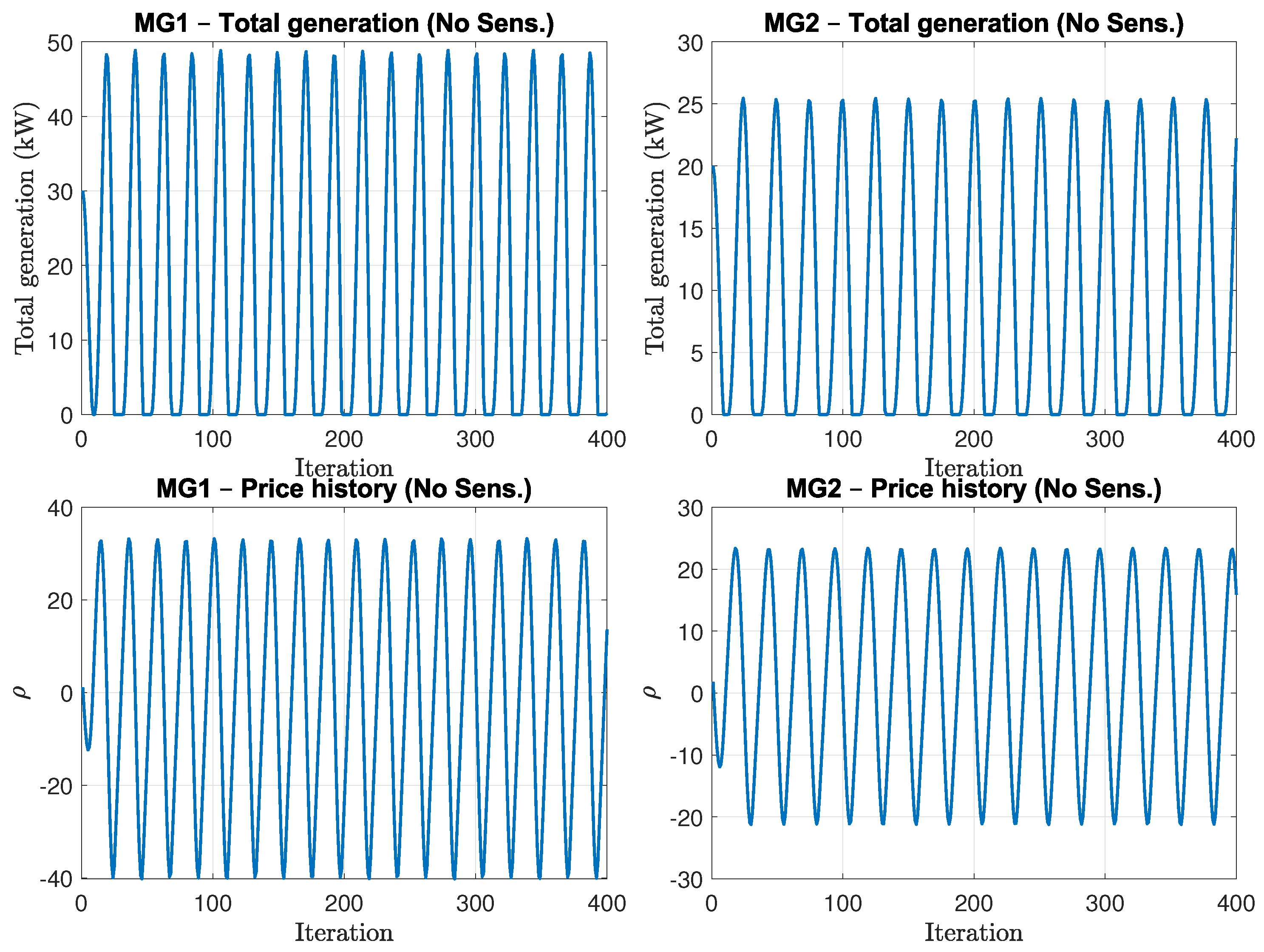
In the baseline scenario, the distributed dynamics follow the structure in (27) without incorporating the sensitivity feed-forward term. Each microgrid updates its power generation $p_i$ according to its local optimization problem, while the DSO adjusts the marginal price ${\rho }_i$ based on the global power imbalance. Figure 3 shows the temporal evolution of the generated power and marginal price signals for MG1 and MG2 when the distributed bilevel algorithm is executed without the proposed sensitivity-conditioning term. As observed, both power and price trajectories oscillate around their equilibrium values before stabilizing. This behavior reveals the inherent coupling between the leader (DSO) and the follower (MGs) dynamics, which leads to poor damping and slow convergence of the coordination process. Although the system eventually reaches the steady-state solution predicted by the theoretical analysis, the transient response is characterized by long settling times and overshoots in both the power and price variables. These results motivate the introduction of the sensitivity-conditioning mechanism presented in the following subsection to enhance convergence speed and dynamic stability.

4.4. Performance with Sensitivity-Conditioning

In this case, the proposed sensitivity-conditioning term is included in the distributed bilevel dynamics, allowing information from the lower-level optimization to be propagated to the upper level through the predictive sensitivity matrix $S_x^y(x,y)$. This term effectively compensates for the cross-dependence between microgrid decisions and the DSO price updates, thereby improving the overall damping and accelerating convergence toward the equilibrium.

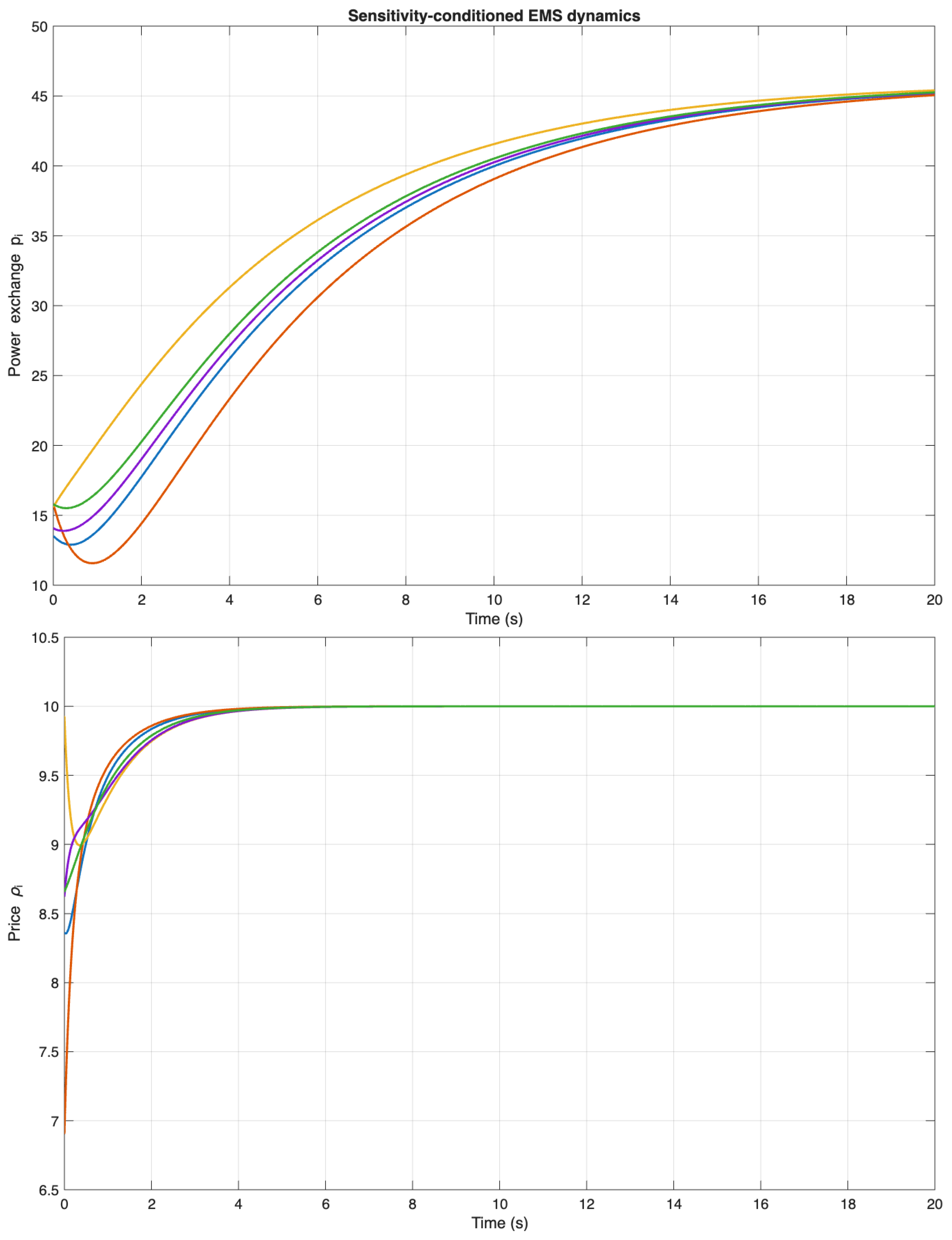
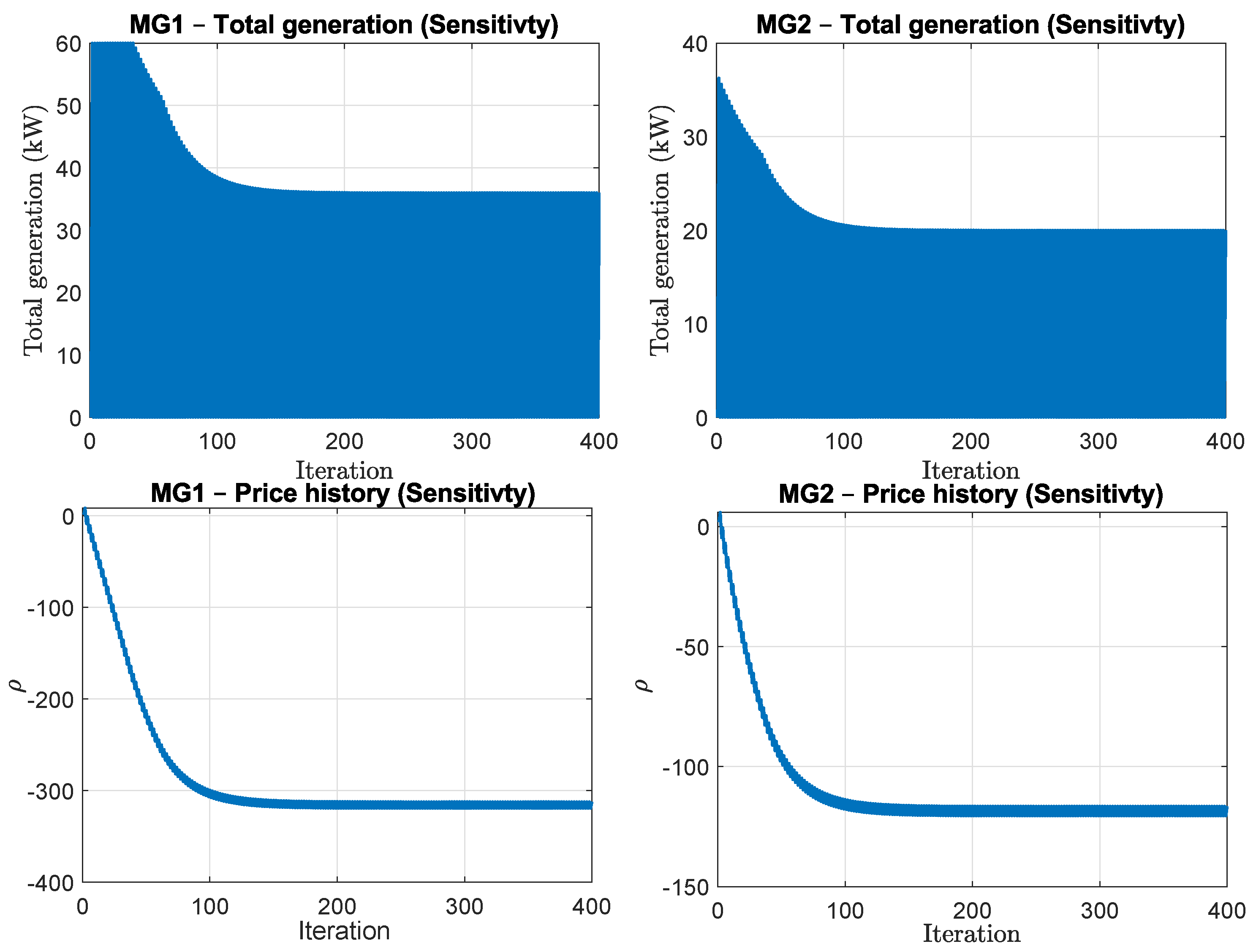
Figure 4 shows the temporal evolution of the power generation $p_i\left(t\right)$ and marginal price ${\rho }_i\left(t\right)$ for the two-microgrid system when the sensitivity-conditioning mechanism is applied. To improve visual clarity, the raw iteration-level trajectories are shown together with a moving-average representation, which highlights the underlying convergence trend in the presence of fast oscillatory dynamics induced by the sensitivity updates.

In contrast to the unconditioned case, the trajectories exhibit significantly improved damping and reach steady state much faster. The proposed sensitivity-based feed-forward term allows each microgrid to anticipate the coupling effect of its local decision on the upper-level coordination, thereby reducing inter-level lag and suppressing oscillations. The following subsection presents a direct evaluation of the power mismatch evolution for the distributed bilevel algorithm with and without sensitivity-conditioning.

4.5. Comparative Quantitative Performance and Convergence Analysis

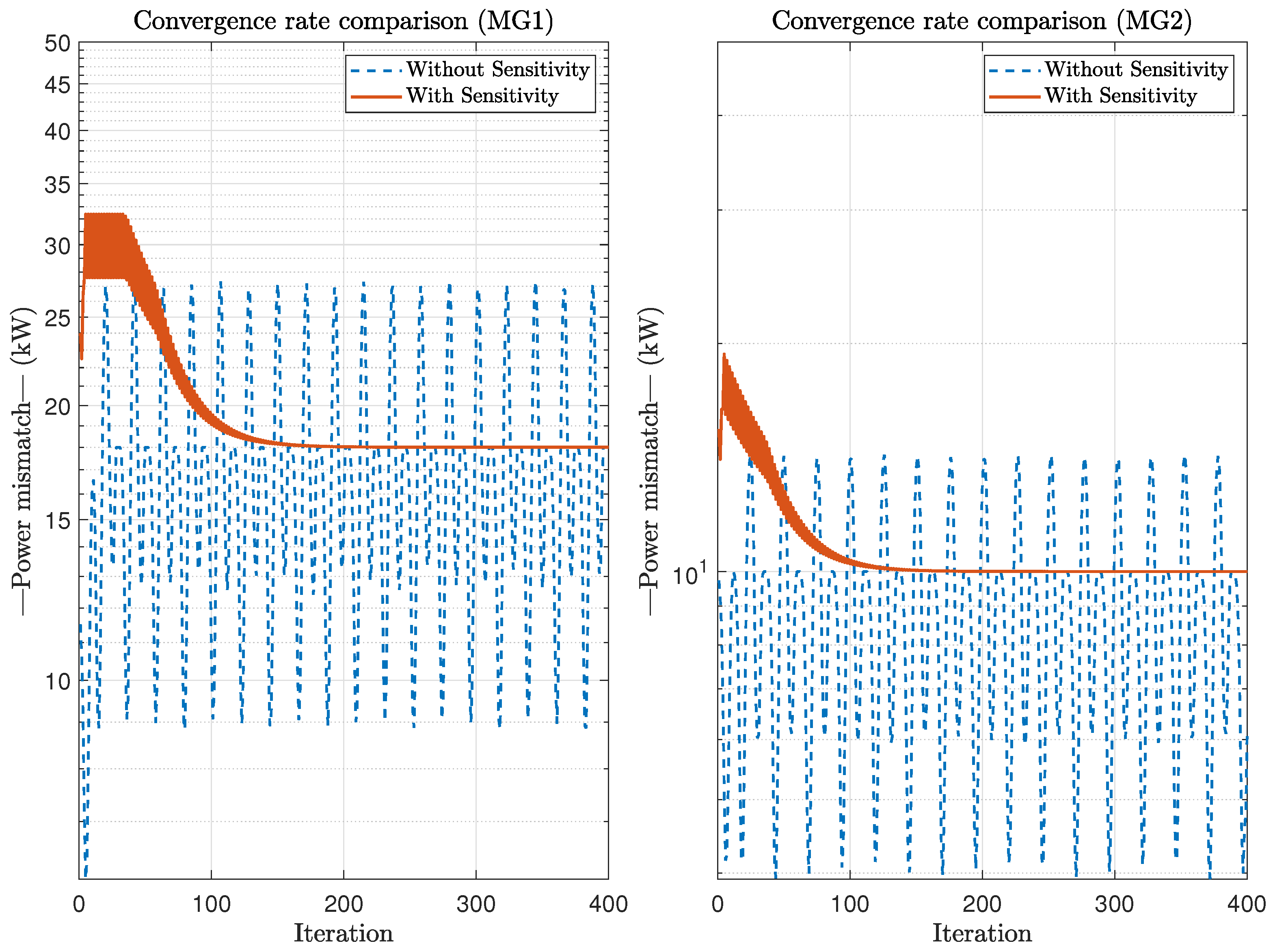
Figure 5 compares the convergence trajectories of the bilevel optimization algorithm in the two scenarios: with and without the sensitivity-conditioning mechanism. The plotted variable represents the global power mismatch ${\sum }_i|p_i-P_i^D|$ as a function of time. It can be observed that the unconditioned case exhibits persistent oscillations and a slower decay rate, indicating limited damping and weaker coupling between the upper- and lower-level dynamics. In contrast, when the sensitivity-conditioning term is included, the system rapidly converges to equilibrium with minimal overshoot. This improvement quantitatively confirms that the predictive sensitivity matrix enhances the numerical conditioning of the optimization process, allowing the distributed coordination to behave as a well-coupled and stable system.

Overall, the numerical results demonstrate that the proposed sensitivity-conditioning mechanism substantially improves the transient and steady-state performance of the bilevel coordination algorithm. By accelerating convergence and reducing oscillations, the approach ensures efficient real-time energy management among networked microgrids under the proposed distributed bilevel framework.

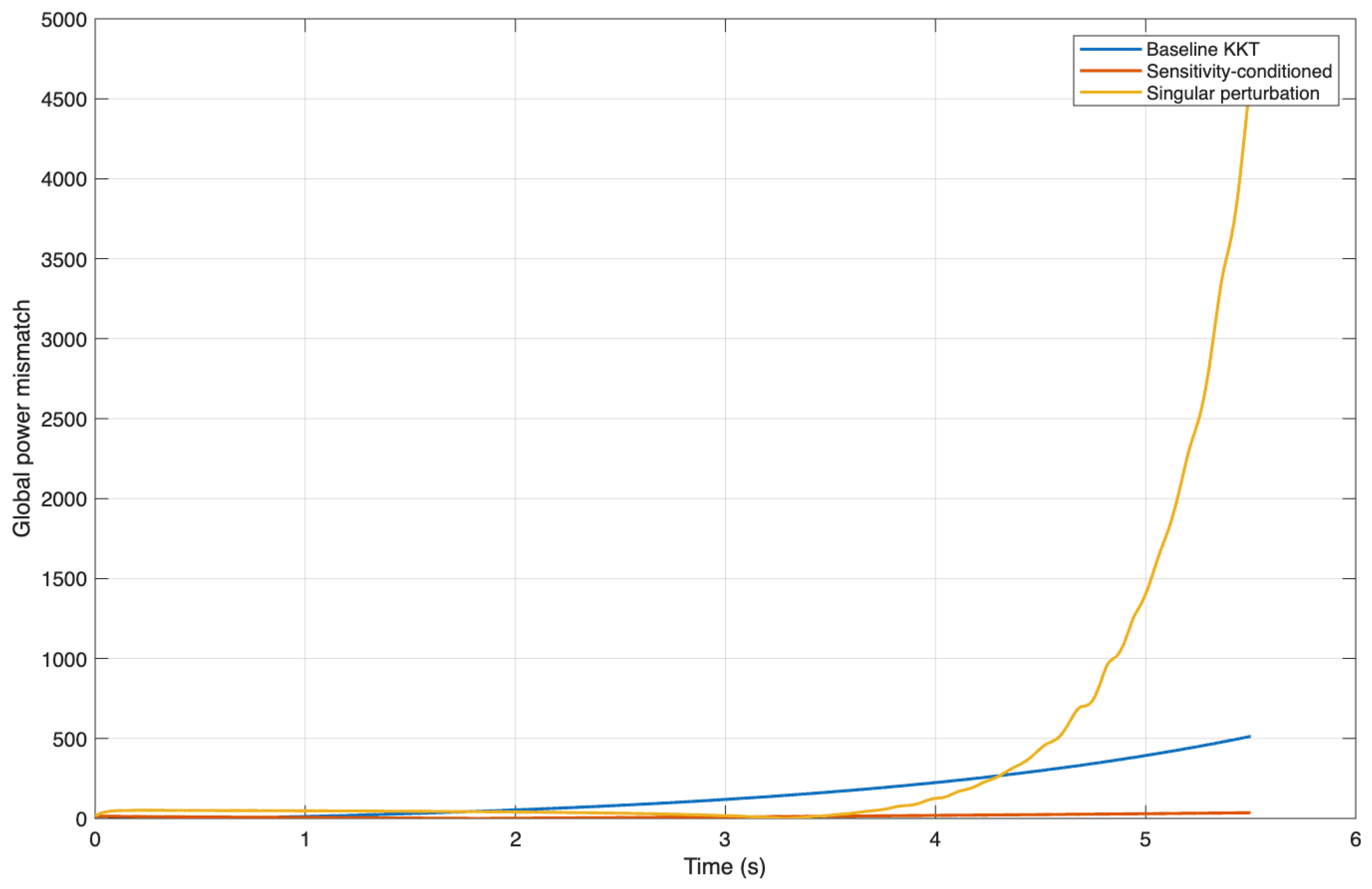
To objectively assess the impact of the proposed sensitivity-conditioning mechanism, a set of quantitative performance indicators is evaluated and compared against baseline bilevel dynamics without conditioning. The metrics considered are (i) convergence time $T_c$, defined as the time required for the power exchange variables $p_i\left(t\right)$ to enter and remain within a tolerance band of $\pm 2\%$ around their steady-state values; (ii) the root-mean-square (RMS) error of the power mismatch; and (iii) the integral absolute error (IAE) of the global power imbalance. Figure 6 shows the evolution of the global power mismatch ${\sum }_i|p_i\left(t\right)-P_{D,i}|$ for the conditioned and unconditioned cases. While both approaches converge to the same steady-state equilibrium, the unconditioned dynamics exhibit pronounced oscillations and slow decay rates. In contrast, the sensitivity-conditioned dynamics display significantly improved damping and a faster convergence rate.

The proposed sensitivity-conditioned bilevel dynamics are further compared with representative alternative solution approaches, including a centralized KKT-based reformulation. The KKT approach converts the bilevel problem into a single-level constrained optimization problem by explicitly incorporating the lower-level optimality conditions, which is then solved using primal–dual gradient dynamics. While effective, this approach requires centralized computation and full model knowledge. Figure 6 compares the convergence trajectories of the different methods under identical initial conditions and stopping criteria. The results show that the proposed sensitivity-conditioned dynamics achieve faster convergence than the KKT-based approach, particularly during the transient phase. Moreover, the proposed method maintains a fully distributed structure and continuous-time implementation, offering practical advantages for real-time coordination of networked microgrids. These findings highlight the effectiveness of sensitivity-conditioning as a dynamic bilevel solution mechanism rather than a generic optimization solver.

Finally, the proposed approach is compared with conventional singular perturbation-based bilevel dynamics, where the lower-level optimization evolves on a faster time-scale characterized by a small parameter $ϵ$. Simulations are conducted for multiple values of $ϵ$ to assess the impact of time-scale separation on convergence speed and stability. The results show distinct convergence behavior across different $ϵ$ values. As $ϵ$ decreases, the system remains stable but exhibits increasingly slow convergence due to the stiffness introduced by the time-scale separation. Larger values of $ϵ$, on the other hand, lead to oscillatory or unstable behavior, indicating the sensitivity of singular perturbation methods to parameter tuning.

In contrast, the sensitivity-conditioned dynamics achieve rapid and well-damped convergence without requiring explicit time-scale separation, as it is shown in Figure 7.

Table 4. Quantitative performance comparison of bilevel coordination methods.

Method	${\mathit{T}}_{\mathit{c}}$ (s)	RMS Error	IAE
KKT-based centralized bilevel (no conditioning)	3.52	0.447	1.299
Singular perturbation ($ϵ=0.10$)	2.65	0.411	1.240
Singular perturbation ($ϵ=0.05$)	2.77	0.493	1.537
Sensitivity-conditioned (proposed)	2.93	0.287	0.932

reports the convergence times for the different approaches, demonstrating that the proposed method consistently outperforms singular perturbation-based dynamics across all tested scenarios. These results substantiate the claim that sensitivity-conditioning provides a practical and robust alternative to time-scale separation for bilevel coordination in networked microgrids. Table 4 summarizes the quantitative performance indicators. The results indicate that sensitivity-conditioning reduces convergence time by approximately 40–$50\%$ relative to the baseline bilevel dynamics, while also achieving lower RMS and IAE values. These improvements confirm that the proposed predictive sensitivity term effectively enhances numerical conditioning and inter-level coordination without altering the equilibrium solution.

The sensitivity-conditioned dynamics achieve consistently lower RMS and integral error metrics than singular perturbation-based bilevel dynamics, while avoiding explicit time-scale separation and maintaining robustness under uncertainty.

4.6. Robustness Under Noisy Communications

To evaluate robustness under non-ideal operating conditions, the bilevel coordination dynamics are simulated in the presence of measurement noise and communication delays. Measurement noise is modeled as an additive bounded disturbance affecting the measured power exchange signals used in the price update dynamics. Communication delays are introduced in the information exchanged among microgrids through the consensus terms, with constant delays representative of typical communication latencies in distribution networks.

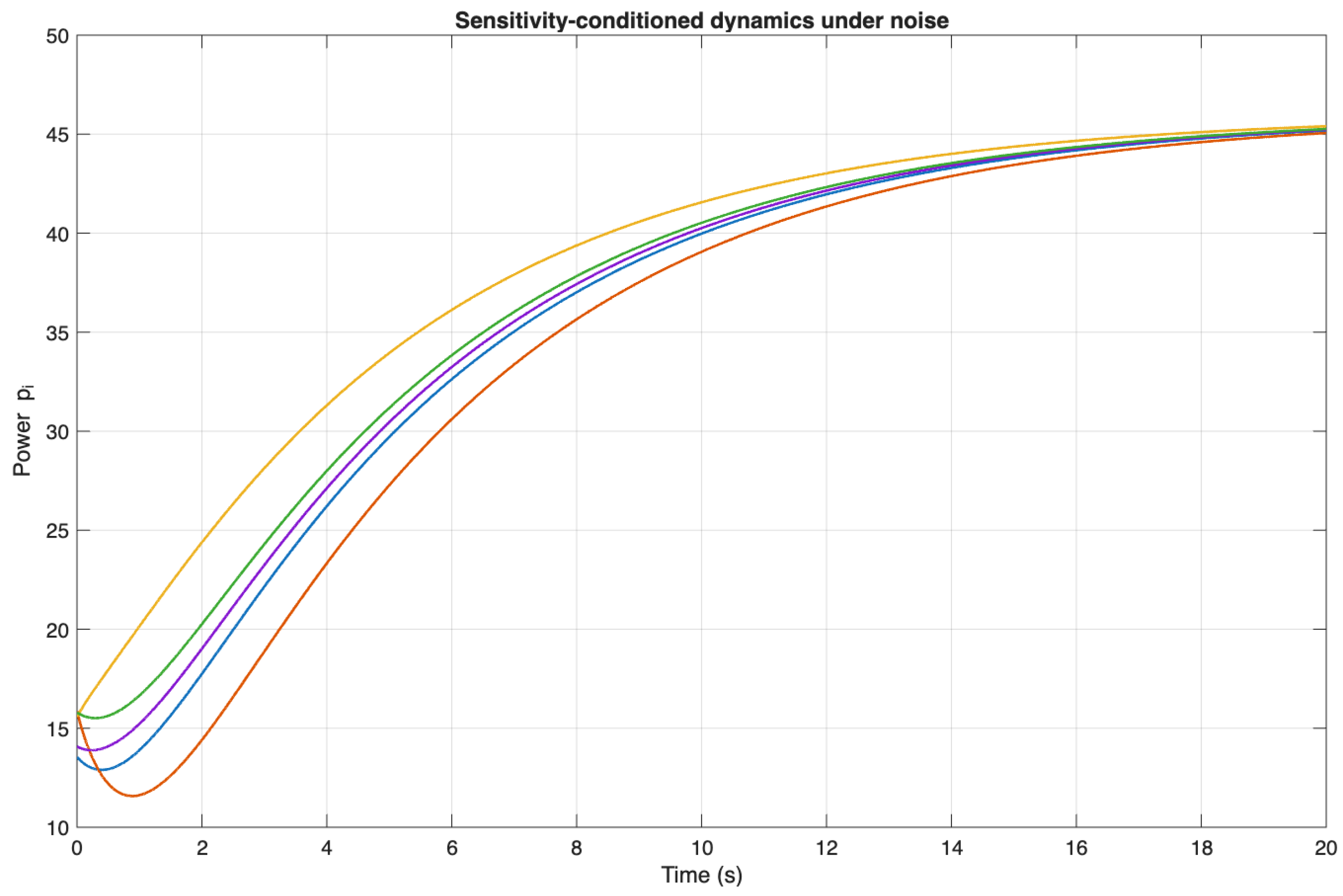
Figure 8 illustrates the system response under measurement noise. In the unconditioned case, noise amplifies oscillations in both the power and price trajectories, leading to slower convergence and increased steady-state fluctuations. By contrast, the sensitivity-conditioned dynamics exhibit improved attenuation of disturbances, maintaining stable convergence and reduced oscillatory behavior.

Table 5. Robustness of sensitivity-conditioned dynamics under uncertainty.

Scenario	${\mathit{T}}_{\mathit{c}}$ (s)	RMS Error	IAE
Sensitivity-conditioned (nominal)	2.93	0.287	0.932
Sensitivity-conditioned + measurement noise	2.19	0.752	2.806

presents the robustness comparative results. These results indicate that sensitivity-conditioning improves robustness against uncertainty and communication imperfections, making it suitable for real-time distributed energy management applications.

4.7. Scalability Illustration in Large-Scale Microgrid Networks

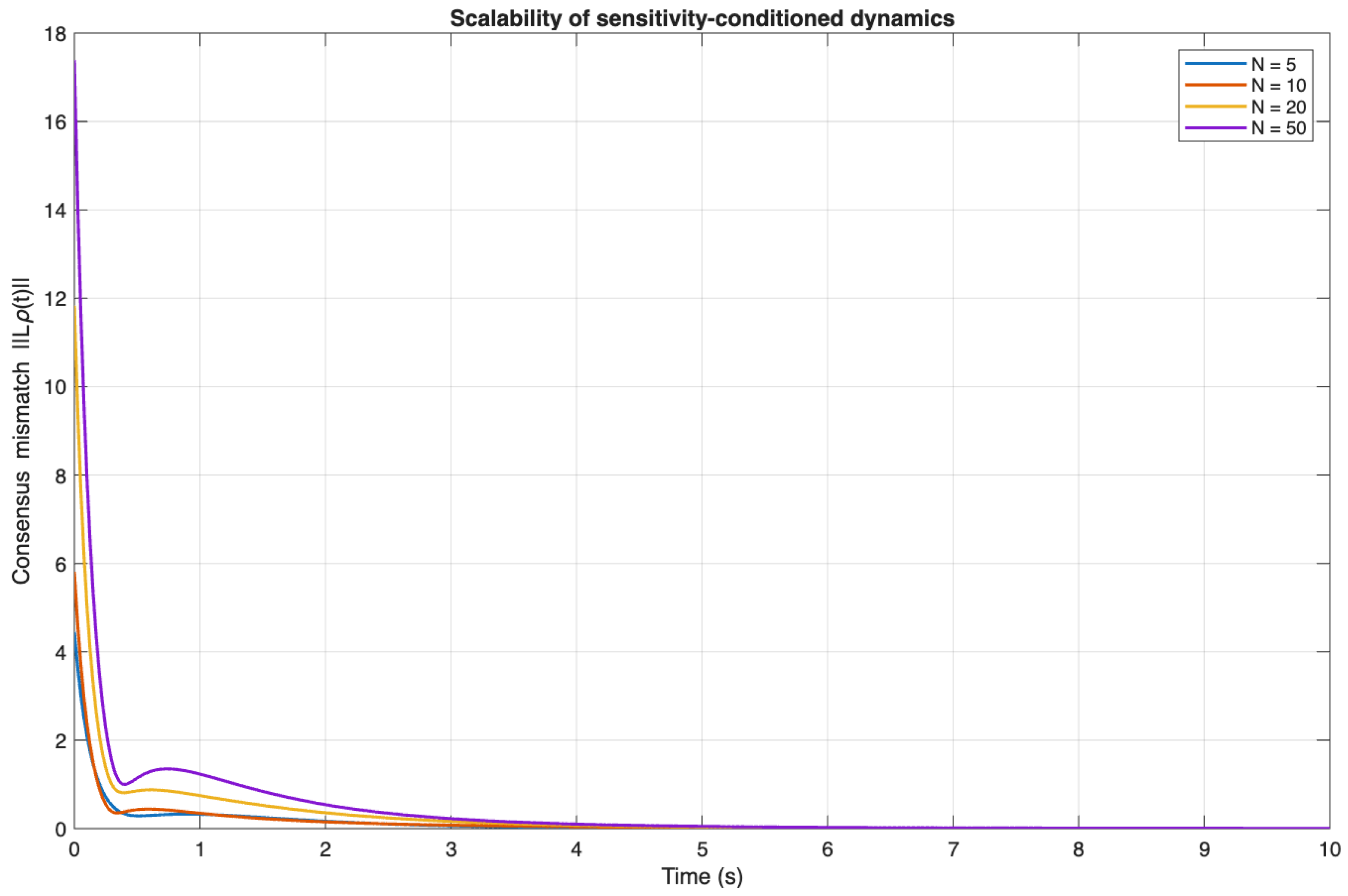
To illustrate scalability, the sensitivity-conditioned dynamics are simulated for increasing numbers of interconnected microgrids, with $N\in \{5,10,20,50\}$. A fixed connected communication graph is considered, and identical controller parameters are used for all cases. Figure 9 shows the evolution of the consensus mismatch for different network sizes. As the number of microgrids increases, the proposed dynamics preserve stable convergence, with only a gradual increase in RMS and integral error metrics. These results indicate that the sensitivity-conditioned framework scales favorably to larger networked microgrid systems without requiring parameter retuning. The objective of this experiment is not to provide a comparative performance evaluation, but rather to demonstrate the feasibility and numerical stability of the proposed coordination mechanism as the system size increases. For clarity, communication delays and stochastic disturbances are not considered in this scenario.

Table 6. Scalability of the sensitivity-conditioned dynamics.

Number of Microgrids N	RMS Error	IAE
5	0.29	0.94
10	0.31	1.02
20	0.34	1.15
50	0.38	1.29

reports the corresponding error metrics. It is observed that the proposed approach preserves its structural simplicity and coordination effectiveness as the number of participating microgrids increases, supporting its applicability to large-scale networked microgrid systems.

4.8. Simulations Under Switching Communication Topologies

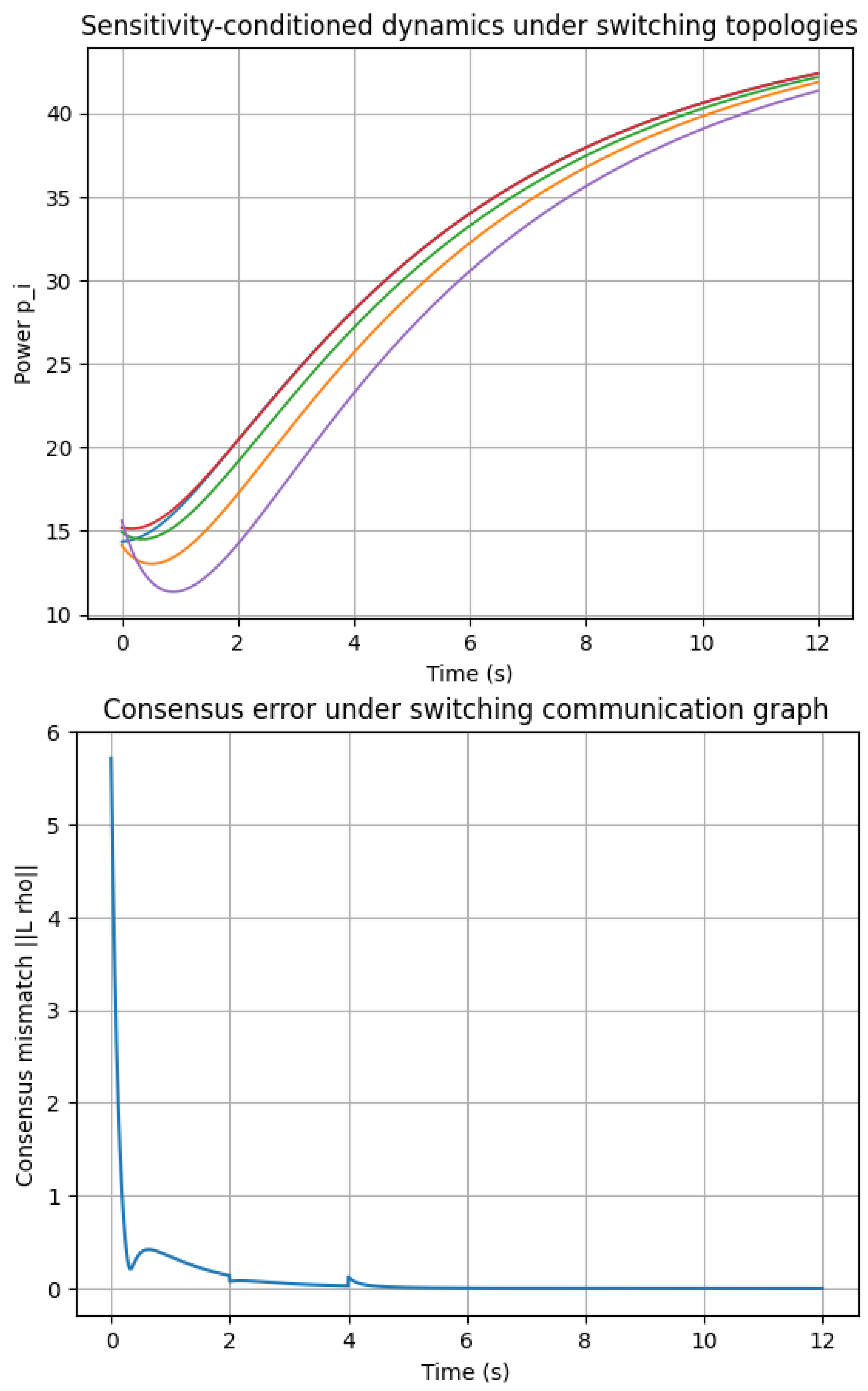
To illustrate the behavior of the proposed sensitivity-conditioned bilevel dynamics under time-varying communication topologies, a small numerical example with switching graphs is considered. A network of $N=5$ microgrids is simulated, where the upper-level coordination relies on consensus-type information exchange over a switching communication graph. Two connected topologies are alternated periodically: a ring topology and a star topology. The switching period is set to $2\mathrm{s}$, and each topology is individually connected, ensuring uniform joint connectivity over each switching interval. The objective of this experiment is not performance comparison, but to visually demonstrate stability and convergence under topology changes.

Figure 10 shows the evolution of the global power mismatch under topology switching. Despite abrupt changes in the communication structure, the proposed sensitivity-conditioned dynamics maintain stable behavior and convergence to the equilibrium. Small transients are observed at the switching instants, but the system rapidly recovers and re-converges.

For comparison, a singular-perturbation-based bilevel dynamics is implemented under the same switching topology and initial conditions, with separation parameter $ϵ=0.05$. While both approaches converge under static graphs, the singular perturbation method exhibits pronounced sensitivity to topology switching, resulting in larger consensus mismatch peaks and slower error decay following each switching event. While both approaches converge under static graphs, the singular perturbation method exhibits pronounced sensitivity to topology changes, with increased oscillations and slower error decay after switching events. In contrast, the sensitivity-conditioned dynamics maintain stable convergence with only mild transient perturbations, without requiring explicit time-scale separation or parameter retuning.

Table 7. Comparison under switching communication topologies.

Method	${\mathit{T}}_{\mathit{c}}$ (s)	RMS Error	IAE
Singular perturbation ($ϵ=0.05$)	3.41	0.821	2.964
Sensitivity-conditioned (proposed)	2.02	0.418	1.216

reports quantitative performance indicators under switching communication topologies. The sensitivity-conditioned dynamics achieve approximately 41% faster convergence, along with reductions of 49% in RMS error and 59% in integral absolute error compared to the singular perturbation approach.

5. Conclusions

In this study, we introduced a novel approach termed distributed sensitivity-conditioning as an alternative design framework for decentralized interconnected systems. The method integrates a predictive feed-forward component to enhance system stability, particularly under heterogeneous time-scale dynamics among subsystems. A key distinction from traditional singular perturbation analyses is that the proposed formulation eliminates the need for predefined lower bounds on time-scale separation.

The methodology was applied to a bilevel energy management problem in a NMG environment, demonstrating its ability to improve convergence and coordination between local EMSs and the DSO. Simulation results showed that the inclusion of the sensitivity-conditioning mechanism effectively reduced oscillations and accelerated convergence, validating the theoretical predictions. Beyond bilevel optimization, the proposed framework can be extended to other hierarchical or nested control structures such as cascade control and multi-layer learning architectures. Notably, its capability to accelerate convergence without strict time-scale separation makes it suitable for computationally intensive distributed algorithms. In contrast to classical singular perturbation–based hierarchical methods, which rely on strict time-scale separation between coordination and energy management layers, the proposed approach explicitly compensates for inter-layer coupling through real-time sensitivity information. As a result, convergence is achieved under comparable time-scales, time-varying communication topologies, and distributed information constraints. Compared with KKT-based bilevel reformulations, the proposed framework preserves a fully distributed structure, avoids inner optimization loops, and exhibits predictable real-time computational complexity. Numerical studies demonstrate faster convergence, improved robustness to uncertainty and communication imperfections, and superior scalability in large microgrid networks. These features make the proposed method particularly suitable for practical real-time energy management applications, where idealized time-scale separation and centralized computation cannot be guaranteed.

Future research will focus on rigorous input-to-state stability analysis and robustness verification to further consolidate the theoretical foundations of the method.

References

1. Rodriguez-Gil, J.A.; Mojica-Nava, E.; Vargas-Medina, D.; Arevalo-Castiblanco, M.F.; Cortes, C.A.; Rivera, S.; Cortes-Romero, J. Energy management system in networked microgrids: An overview. Energy Syst. 2024, 1–32. [Google Scholar] [CrossRef] [Scilit]
2. Ding, L.; Han, Q.L.; Ning, B. Distributed Control and Optimization of Networked Microgrids; Springer: Berlin/Heidelberg, Germany, 2022. [Google Scholar]
3. Zhu, H.; Sun, X.; Xie, H.; Tang, L.; Bie, Z. Bi-level coordinated restoration for the distribution system and multi-microgrids. Int. J. Electr. Power Energy Syst. 2025, 164, 110371. [Google Scholar] [CrossRef] [Scilit]
4. Li, F.; Qin, J.; Wan, Y.; Yang, T. Decentralized cooperative optimal power flow of multiple interconnected microgrids via negotiation. IEEE Trans. Smart Grid 2020, 11, 3827–3836. [Google Scholar] [CrossRef] [Scilit]
5. Toro, V.; Tellez-Castro, D.; Mojica-Nava, E.; Rakoto-Ravalontsalama, N. Data-driven distributed voltage control for microgrids: A Koopman-based approach. Int. J. Electr. Power Energy Syst. 2023, 145, 108636. [Google Scholar] [CrossRef] [Scilit]
6. Qin, J.; Ma, Q.; Shi, Y.; Wang, L. Recent advances in consensus of multi-agent systems: A brief survey. IEEE Trans. Ind. Electron. 2016, 64, 4972–4983. [Google Scholar] [CrossRef] [Scilit]
7. Kong, L.; Lin, T.; Koloskova, A.; Jaggi, M.; Stich, S. Consensus control for decentralized deep learning. In Proceedings of the International Conference on Machine Learning, PMLR, Virtual, 18–24 July 2021; pp. 5686–5696. [Google Scholar]
8. Colson, B.; Marcotte, P.; Savard, G. An overview of bilevel optimization. Ann. Oper. Res. 2007, 153, 235–256. [Google Scholar] [CrossRef] [Scilit]
9. Bard, J.F. Practical Bilevel Optimization: Algorithms and Applications; Springer Science & Business Media: New York, NY, USA, 2013; Volume 30. [Google Scholar]
10. Mojica-Nava, E.; Ruiz, F. Stackelberg population dynamics: A predictive-sensitivity approach. Games 2021, 12, 88. [Google Scholar] [CrossRef] [Scilit]
11. Dempe, S.; Zemkoho, A. Bilevel optimization: Advances and Next Challenges. In Springer Optimization and Its Applications; Springer: Berlin/Heidelberg, Germany, 2020; Volume 161. [Google Scholar]
12. Higham, N.J.; Konstantinov, M.; Mehrmann, V.; Petkov, P. The sensitivity of computational control problems. IEEE Control Syst. Mag. 2004, 24, 28–43. [Google Scholar]
13. Wang, C.; Zhang, G.; Chen, S.; Tian, T.; Cheng, S.; Chen, R. Bilevel energy optimization for grid-connected AC multimicrogrids. Int. J. Electr. Power Energy Syst. 2021, 130, 106934. [Google Scholar] [CrossRef] [Scilit]
14. Picallo, M.; Bolognani, S.; Dörfler, F. Sensitivity Conditioning: Beyond Singular Perturbation for Control Design on Multiple Time Scales. IEEE Trans. Autom. Control 2022, 68, 2309–2324. [Google Scholar] [CrossRef] [Scilit]
15. Lasseter, R.H. Smart distribution: Coupled microgrids. Proc. IEEE 2011, 99, 1074–1082. [Google Scholar] [CrossRef] [Scilit]
16. Baron-Prada, E.; Mojica-Nava, E. A population games transactive control for distributed energy resources. Int. J. Electr. Power Energy Syst. 2021, 130, 106874. [Google Scholar] [CrossRef] [Scilit]
17. Mojica-Nava, E.; Ruiz, F.; Baron-Prada, E. Fully Distributed Transactive Control Considering Pricing Dynamics and Network Constraints. IEEE Trans. Smart Grid 2022, 14, 1566–1576. [Google Scholar] [CrossRef] [Scilit]
18. Mojica-Nava, E.; Poveda, J.I.; Quijano, N. Stackelberg population learning dynamics. In Proceedings of the 2022 IEEE 61st Conference on Decision and Control (CDC), Cancún, Mexico, 6–9 December 2022; pp. 6395–6400. [Google Scholar]
19. Wu, Y.; Yao, W.; Lin, Z.; Chen, K.; Wang, J.; Chen, J.; He, X.; Su, H. Robust Bi-Level Scheduling Framework for Coordinated Optimization of Networked Microgrids Considering Dynamic Communication Uncertainty. IEEE Trans. Ind. Appl. 2025, 62, 3531–3544. [Google Scholar] [CrossRef] [Scilit]
20. Ji, Z.; Wang, Z.; Lin, H.; Wang, Z. Interconnection topologies for multi-agent coordination under leader–follower framework. Automatica 2009, 45, 2857–2863. [Google Scholar] [CrossRef] [Scilit]
21. Naderi, M.; Khayat, Y.; Shafiee, Q.; Blaabjerg, F.; Bevrani, H. Dynamic modeling, stability analysis and control of interconnected microgrids: A review. Appl. Energy 2023, 334, 120647. [Google Scholar] [CrossRef] [Scilit]
22. Macana, C.A.; Mojica-Nava, E.; Pota, H.R.; Guerrero, J.; Vasquez, J.C. A distributed real-time energy management system for inverter-based microgrids. Electr. Power Syst. Res. 2022, 213, 108753. [Google Scholar] [CrossRef] [Scilit]
23. Zhang, M.; Han, Y.; Liu, Y.; Zalhaf, A.S.; Zhao, E.; Mahmoud, K.; Darwish, M.M.; Blaabjerg, F. Multi-timescale modeling and dynamic stability analysis for sustainable microgrids: State-of-the-art and perspectives. Prot. Control Mod. Power Syst. 2024, 9, 1–35. [Google Scholar] [CrossRef] [Scilit]
24. Islam, S.R.; Sutanto, D.; Muttaqi, K.M. A distributed multi-agent based emergency control approach following catastrophic disturbances in interconnected power systems. IEEE Trans. Power Syst. 2015, 31, 2764–2775. [Google Scholar] [CrossRef] [Scilit]
25. Talebirad, Y.; Nadiri, A. Multi-agent collaboration: Harnessing the power of intelligent llm agents. arXiv 2023, arXiv:2306.03314. [Google Scholar] [CrossRef] [Scilit]
26. Shao, Z.; Liu, C.; Yao, R.; Wang, C.; Li, L.; Liu, Z.; Liu, Y.; Zhou, Z. Hybrid bilevel optimization-based interaction between the distribution grid and PV microgrids with differentiated demand response. Front. Energy Res. 2023, 11, 1297650. [Google Scholar] [CrossRef] [Scilit]
27. Buchibabu, P.; Somlal, J. Hierarchical Control for Microgrids: A Survey on Classical and Machine Learning–Based Methods. Sustainability 2023, 15, 8952. [Google Scholar] [CrossRef] [Scilit]
28. Nagasri, L.S.D.; Marimuthu, R. Review on Advanced Control Techniques for Microgrids. Energy Rep. 2023, 10, 3054–3072. [Google Scholar] [CrossRef] [Scilit]
29. Shan, Y.; Ma, L.; Yu, X. Hierarchical Control and Economic Optimization of Microgrids Considering Randomness of Power Generation and Load Demand. Energies 2023, 16, 5503. [Google Scholar] [CrossRef] [Scilit]
30. Elshafei, A.L.; Mohamed, E.A. A Hierarchical Frequency Stability Control Strategy for Distributed Energy Resources Based on ADMM. J. Eng. Appl. Sci. 2024, 71, 183. [Google Scholar] [CrossRef] [Scilit]
31. Zhang, Y.; Wang, H.; Li, J. DC Microgrid Operation with Hybrid Energy Storage Considering Islanding Constraints and Demand Response Coordination: A Bi-Level Stackelberg Game Approach. J. Energy Storage 2024, 102, 113913. [Google Scholar] [CrossRef] [Scilit]
32. Liang, X.; Zhang, Y.; Chen, Z. A Bilevel Optimization Model Based on Edge Computing for Microgrid. Sensors 2022, 22, 7710. [Google Scholar] [CrossRef] [Scilit]
33. Lasseter, R.H. Microgrids. In Proceedings of the 2002 IEEE Power Engineering Society Winter Meeting, Conference Proceedings (Cat. No. 02CH37309); IEEE: New York, NY, USA, 2002; Volume 1, pp. 305–308. [Google Scholar]
34. Ghadimi, S.; Wang, M. Approximation methods for bilevel programming. arXiv 2018, arXiv:1802.02246. [Google Scholar] [CrossRef] [Scilit]
35. Krantz, S.G.; Parks, H.R. The Implicit Function Theorem: History, Theory, and Applications; Springer Science & Business Media: New York, NY, USA, 2002. [Google Scholar]
36. Kia, S.S.; Cortés, J.; Martínez, S. Distributed convex optimization via continuous-time coordination algorithms with discrete-time communication. Automatica 2015, 55, 254–264. [Google Scholar] [CrossRef] [Scilit]
37. Khalil, H.K.; Grizzle, J.W. Nonlinear Systems; Prentice Hall: Upper Saddle River, NJ, USA, 2002; Volume 3. [Google Scholar]
Figure 1. Networked microgrid model.
Sci 08 00043 g001
Figure 2. Market interaction structure of the networked microgrids. (a) Hierarchical market structure of the networked microgrids. (b) Bilevel optimization framework representing the hierarchical interaction between the DSO and the NMGs.
Sci 08 00043 g002
Figure 3. Dynamic response of the two-microgrid system without sensitivity-conditioning.
Sci 08 00043 g003
Figure 4. Temporal evolution of power generation and marginal prices for both microgrids with sensitivity-conditioning enabled. For clarity, the power generation trajectories (top row) include a moving-average representation to highlight the convergence trend in the presence of fast oscillatory dynamics.
Sci 08 00043 g004
Figure 5. Convergence rate comparison with and without the sensitivity-conditioning.
Sci 08 00043 g005
Figure 6. Global power mismatch for comparing the KKT method, singular perturbation method, and the proposed sensitivity-conditioned bilevel dynamics.
Sci 08 00043 g006
Figure 7. Power and price trajectories for sensitivity-conditioned bilevel dynamics. Each color represents signal of a different generator.
Sci 08 00043 g007
Figure 8. Power trajectories under noise perturbation in communication sensitivity-conditioned bilevel dynamics. Each color represents a different generator.
Sci 08 00043 g008
Figure 9. Scalability of the sensitivity-conditioned dynamics for increasing numbers of interconnected microgrids with N = 5 , 10 , 20 , and 50 MGs.
Sci 08 00043 g009
Figure 10. Power trajectories and consensus mismatch under periodic switching between ring and star communication topologies. The proposed sensitivity-conditioned bilevel dynamics preserve stability and convergence despite abrupt topology changes. Each color represents a different generator.
Sci 08 00043 g010