Abstract
This study presents the geometric optimization of a Savonius-type VAWT with multi-element blade profiles using a full factorial design integrated with RSM. Two crucial geometric parameters, the blade twist angle () and the aspect ratio (), were systematically varied to assess their influence on the power coefficient (). Experimental measurements were performed in a controlled wind tunnel environment, and a second-order regression equation was used to model the resulting data. The optimization approach identified the combination of and that maximized . The optimal configuration was achieved with a of 30° and an of 2.0, for which the experimentally measured power coefficient () reached a value of 0.2326. The results confirm that lower twist angles and higher aspect ratios enhance aerodynamic efficiency, reduce manufacturing complexity, and improve structural reliability. These findings highlight the potential of Savonius turbines as competitive solutions for small-scale energy harvesting in low-wind-speed environments. Moreover, the identified optimal configuration provides a basis for future work that focuses on scaling the design, integrating power transmission and electrical generation components, and validating performance under real operating conditions.
1. Introduction
As societies grow and their dependence on technology intensifies, fossil-fuel-based energy production is becoming increasingly unviable [1,2,3]. Therefore, shifting toward renewable sources, such as wind, has become essential [4,5,6]. Renewable sources offer more sustainable alternatives to meet energy demands, minimize the effects of climate change, and reduce greenhouse gas emissions [7,8,9]. Wind turbines play an important role in diversifying the energy mix, providing unique benefits while presenting specific engineering and environmental challenges [10,11]. Their relatively low environmental footprint, modularity, and scalability make them suitable for a broad variety of uses [12,13]. However, several challenges must be addressed to maximize their potential. The intermittency of wind remains a primary limitation as energy output fluctuates with atmospheric conditions [14]. Additionally, questions related to noise pollution, visual impact, and potential disruption to local wildlife must be considered [15,16]. Integrating wind energy into existing power grids presents technical challenges, especially regarding the demand for efficient energy storage systems. The initial investment and maintenance costs of wind systems can be significant, particularly in remote or offshore installations [17,18]. Despite these limitations, wind turbines have significant potential for providing sustainable and varied energy options.
The classification of wind turbines is largely based on the orientation of their rotational axis, resulting in two principal types: horizontal-axis wind turbines (HAWTs) and vertical-axis wind turbines (VAWTs) [19,20]. In HAWTs, the main rotor shaft is aligned horizontally, parallel to the ground, and typically points into the wind. In contrast, VAWTs have a rotor shaft that is oriented vertically, perpendicular to the ground, allowing them to capture wind from any direction without demanding orientation mechanisms. This makes them particularly suitable for urban areas and environments with complex or unstable wind conditions [20,21].
Vertical-axis wind turbines (VAWTs) have captured interest as a viable alternative to conventional horizontal-axis wind turbines (HAWTs) in renewable energy production [22,23]. HAWTs have traditionally dominated large-scale wind power installations because of their higher efficiency in steady, high-speed wind environments, whereas VAWTs offer distinct advantages in specific scenarios. These include urban areas, complex terrains, and locations where the wind is turbulent, variable, or of lower velocity. Although they are generally less efficient than HAWTs, VAWTs are easier to install and maintain, especially in decentralized or constrained environments, and continue to gain interest as complementary solutions in the landscape of wind energy [23,24].
The development of VAWTs is an active and evolving field of research. To optimize rotor design, researchers employ a combination of numerical simulations and experimental investigations [25]. Computational simulations enable the modeling and prediction of turbine performance under various operating conditions, offering crucial observations of aerodynamic behavior and energy output [11]. Despite these tools’ accuracy, experimental validation remains essential. Controlled physical testing confirms the simulation results and provides critical real-world performance data. Well-equipped experimental setups act as testbeds for evaluating turbine behavior under various flow conditions, closing the gap between theoretical predictions and practical application.
Emphasizing the effects of the blade twist angle (), aspect ratio (), and blade modifications on the power coefficient (), which measures the efficiency of wind energy conversion into mechanical power, the following findings were obtained. Anbarsooz et al. showed that increasing from 0° to 45° reduces from 0.12 to 0.11 but improves torque uniformity [26]. Conversely, higher , such as 180°, as studied by Kothe et al. [27], Jeon et al. [28], and Zadeh et al. [29], offers enhanced startup capabilities and better energy capture when combined with optimized blade geometries. For example, Zadeh et al. [29] reported a of 0.148 using a Bach-profile rotor, while Damak et al. [30] reached the highest of 0.2 by combining Bach and helical features into a hybrid rotor.
strongly affects performance. Kamoji et al. [31] found that a rotor with an of 0.88 and no central shaft reached a of 0.174, outperforming other geometries with higher ARs. Lajnef et al. [32] tested delta and two-stage delta blades with an aspect ratio of 1.25 and a 90° twist, achieving values of 0.148 and 0.152, respectively. Jeon et al. [28], using a higher aspect ratio of 2.0, demonstrated that the addition of circular end plates improved by 36%, though high aspect ratios can complicate structural design and manufacturing. The blade geometry and structural features are key to optimizing rotor performance. Lajnef et al. [33] showed that non-overlapping blades at a 180° twist outperformed overlapped blades, achieving a of 12.4%. Damak et al. [34] concluded that both the Reynolds number and overlap ratio affect rotor performance, with a maximum of 0.2 at a tip speed ratio () of 0.33 and an overlap ratio of 0.242.
Although these studies provide valuable insights, most are limited to specific geometrical configurations or rely primarily on numerical simulations, which may not fully capture the complexity of aerodynamic behavior. Moreover, the combined influence of the aspect ratio and twist angle has rarely been studied in a systematic way, and the parameter ranges explored in previous works are often narrow, restricting the generalization of the results.
In this context, VAWTs represent a versatile and efficient solution for both distributed energy generation and enhancing the resilience of existing power grids. Their ability to operate independently of wind direction and their ease of ground-level installation make them particularly suitable in scenarios where conventional horizontal-axis wind turbines (HAWTs) are not feasible [35]. This study introduces a novel experimental approach focused on optimizing a Savonius-type turbine by incorporating multielement blade profiles, a configuration that has received little attention in the literature, to address the aforementioned gaps. Unlike most prior works, this study combines experimental wind tunnel testing with a full factorial response surface methodology (RSM), allowing the systematic evaluation of two critical parameters—the blade twist angle () and the aspect ratio ()—across a broader range than typically reported. This integrated approach ensures robust validation of the aerodynamic performance and represents an innovative strategy to maximize the power coefficient ().
2. Materials and Methods
2.1. Vertical-Axis Wind Turbines (VAWTs)
VAWTs use the interaction between their rotor blades and the wind to convert kinetic energy into rotational motion, which is subsequently transformed into electricity through a connected generator [36]. In contrast to horizontal-axis wind turbines, VAWTs are capable of harnessing wind from all directions without the need for alignment systems, making them ideal for cities and areas where wind patterns can be unpredictable or turbulent [37,38]. Generally, VAWTs fall into two main categories: drag-based and lift-based turbines, depending on the aerodynamic principle used to generate rotation [24]. Drag-based designs, such as the Savonius turbine, rely on wind resistance acting on curved blades to produce motion. Although their energy conversion efficiency is relatively low, they are simple to build, perform well in low wind conditions, and are suitable for applications where high power output is not critical [39,40].
Lift-based turbines, such as the Darrieus and Gorlov types, generate rotation through aerodynamic lift, offering higher efficiency at elevated wind speeds. The Darrieus turbine has straight airfoil blades but requires external starting mechanisms, whereas the Gorlov turbine’s helical design improves performance and stability in turbulent conditions. Conversely, drag-based designs, such as the Savonius turbine, stand out for shape, causing differential drag that induces rotation [41]. There are two main blade designs: straight and helical blades [42]. While straight blades are easier and cheaper to manufacture, they suffer from greater vibration and torque fluctuations. Although more complex and costly, helical blades enable smoother airflow, reduced turbulence, and quieter operation, which are all advantages that are particularly valuable in urban settings. Savonius turbines typically achieve power coefficients () ranging from 0.15 and 0.30 [42,43,44,45], offering a reliable solution for low-speed wind conditions with minimal installation and maintenance needs.
P denotes the available power, A represents the swept area of the blades, is the fluid density, and V corresponds to the flow velocity. The power coefficient is defined as the ratio of P to the output power (), as shown in Equation (2). In the case of the Savonius turbine, A is calculated as the product of the rotor’s height (H) and its diameter (D), that is, [46].
The generated power is estimated as the product of torque (T) and rotational velocity (), as described by Equation (3) [46]:
In order to characterize the operation of a turbine, it is essential to examine how varies with the relative velocity at the blade tip, which is governed by the tip speed ratio (). is expressed as as the ratio of the blade’s tangential speed at a given instant to the actual speed at the blade tip. Its mathematical expression is provided in Equation (4).
R denotes the radius of the turbine.
2.2. Rotor Design
Figure 1 presents a cross-sectional view of the Savonius rotor with a Bach-type blade profile, where the two primary S-shaped blades and the auxiliary secondary blades are clearly visible. The blade geometry is fully defined in terms of the rotor diameter (D), and the key construction dimensions are indicated. The parameters O, P, and Q represent the characteristic geometric ratios optimized in previous studies to 96.81%, 17.43%, and 9.4% of D, respectively [45,47]. On the right, Detail A provides a magnified view of the secondary blade region, illustrating its positioning and the corresponding dimensional relationships. This schematic highlights the essential design parameters required for the accurate reproduction of the rotor geometry. The use of multielement profiles in the Savonius turbine is intended to increase pressure on the inner blade surface, thereby reducing resistance and enhancing efficiency. The detailed geometric characteristics of the baseline design can be found in the specialized literature.
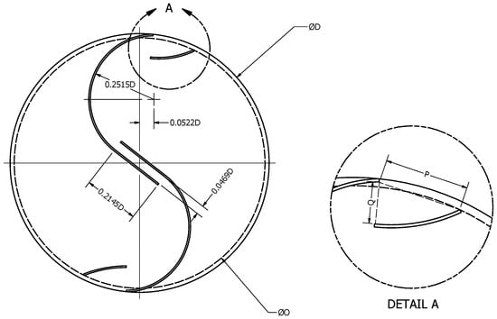
Figure 1.
Cross-sectional view of the Savonius rotor with main and secondary blades.
Savonius turbines are traditionally designed with straight blades, but recent advancements have introduced variations in geometry, such as the use of helical blades [27,29,33]. These modifications aim to enhance aerodynamic performance and efficiency. A comparison between the straight and helical blade geometries is illustrated in Figure 2. Savonius turbines with a helical blades are more complex to manufacture due to the intricate design of the blades. However, this configuration enhances performance by optimizing the interaction between the blades and the airflow. The helical shape ensures continuous engagement with the wind, reducing torque fluctuations and improving efficiency, as the blades consistently harness the air’s force throughout their rotation.
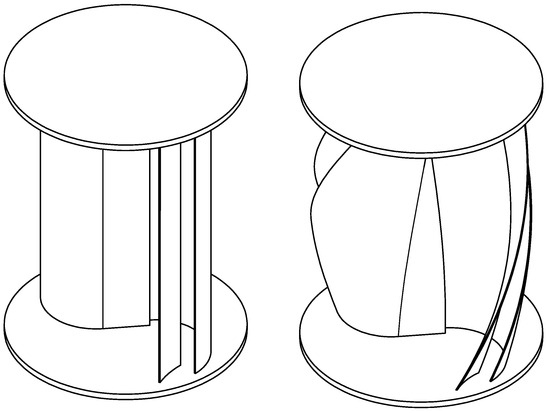
Figure 2.
Savonius rotor with a Bach-type blade profile: straight blade (left) and blade twist angle (right).
Savonius turbine performance is influenced by several key design parameters. One of the most critical is the aspect ratio (), which directly affects aerodynamic behavior and energy capture. Generally, a higher means better performance in changing wind conditions because it allows the rotor to catch more wind energy. is defined as the ratio between H and D [48,49], and it has a critical function in determining the swept area and the overall capacity of the turbine to interact with the wind flow. In the case of the helical Savonius rotors, is a particularly important parameter. This angle determines how the blades are positioned in relation to the wind, which influences how the airflow behaves and how much energy can be collected. More precisely, the blade twist angle () is the angle formed between the projection of the blade’s helical curve and the plane perpendicular to the rotor’s axis [50,51]. An appropriately selected helix angle allows for smoother airflow through the rotor, reducing turbulence, minimizing torque fluctuations, and improving overall efficiency. Both and must be carefully optimized to achieve the best aerodynamic performance, particularly in low-wind-speed and turbulent environments.
2.3. Optimization Methodology
For the rotor optimization phase, RSM was used in combination with a full factorial experimental design. This approach evaluates all possible combinations of the independent variable levels [52,53]. In this case, the two selected factors are and . Three levels were considered for each factor: the aspect ratio was set to 0.7, 1.35, and 2.0, while the blade twist angle was set to 30°, 105°, and 180°. The values or levels of these factors were obtained after analyzing the twist angle and aspect ratio ranges reported by other authors [27,29,30,34,54,55]. Specifically, the values reported in the cited works were tabulated, and the minimum and maximum of those ranges were used as reference limits. In some cases, the lower bound was extended in order to cover a slightly wider range of geometrical configurations and to ensure that the selected values encompassed all the cases analyzed by previous authors. In this way, the proposed ranges are not arbitrary but are physically consistent with existing studies while still broad enough to capture the influence of these parameters on the turbine’s performance. The central level in each factor corresponds to the midpoint between the maximum and minimum values, which is a standard approach in factorial experimental designs.
Full factorial design enables a comprehensive analysis of factor interactions, offering insights into how simultaneous variations in these parameters influence the response variable, namely, the power coefficient (). Such insight is critical as design factors rarely act independently; understanding their combined effects can uncover performance gains not apparent through more limited experimental approaches.
Following the values established in the full factorial design, the geometries were constructed, and a total of nine models were obtained, each corresponding to a unique treatment (i.e., a specific combination of factor levels). The nine models have a fixed D of 200 mm and a wall thickness of 2.5 mm. Table 1 presents the complete set of models to be conducted, organized according to the two key factors along with their corresponding values.

Table 1.
Models.
Upon completing the nine experiments, a regression model can be developed according to the collected data. Various types of functions, such as linear, quadratic, cubic, and other specialized forms, may be applied to create the regression model. Second-order polynomial models are commonly employed, within various fields of engineering [56,57].
Accordingly, Equation (5) describes the general equation for a complete regression model considering the two independent variables [58,59]. In this equation, is the response variable to be maximized; is a constant term; and are the linear coefficients; and represent the quadratic coefficients; and accounts for the interaction effects.
ANOVA was used to analyze the dataset and evaluate the model’s importance of each term. By dividing the total variability in the data into parts associated with different sources, ANOVA helps identify how different geometric parameters influence outcome using a range of descriptive statistics [60,61]. These metrics include p-value, the sum of squares (SS), the mean square of the error (MSE), the total sum of squares (SST), and the F-ratio. These specific metrics measure statistical significance with respect to the null hypothesis, which assumes that no relationship exists between the variables. Conventionally, a p-value below 0.05 (expressed as p < 0.05) is regarded as statistically significant, providing substantial evidence against the null hypothesis and supporting its rejection in favor of the alternative hypothesis [62,63].
The F-ratio is obtained by dividing MS by MSE [64]. In turn, MS is determined by dividing SS by the associated degrees of freedom (df) [65]. The quantifies the volume of data provided by the sample and is defined according to the number of observations; the df assigned to a given term reflects the portion of information consumed by that term. The SST comprises the sum of the SS and SSE treatments, as shown in Equation (6) [56]. Finally, the p-value is obtained from the F-distribution table, considering the selected significance level and corresponding to both the treatment and the error [66].
In this case, predicted the value for the i-th trial, is the mean of the observed response variable values, is the i-th observed value of the response variable, and n is the number of observations. The correlation coefficient () and the adjusted coefficient of determination () were calculated using Equations (7) and (8), following the method outlined by Bouvant et al. [56]. These metrics indicate the extent of data variation captured by the models. The p-value was used to determine the statistical significance of the models in reflecting the experimental outcomes. To visualize how the design factor levels affect , 3D plots were generated. Statistical analysis was performed using the R Project, maintaining a 95% confidence level.
2.4. Wind Tunnel and Data Acquisition System
A wind tunnel is an essential tool for the characterization and analysis of wind turbine designs as it enables the simulation of aerodynamic conditions within a controlled environment. Its importance comes from how well it can mimic wind patterns and flow features, which makes it possible to closely assess how turbines perform and behave in different wind conditions. Through these simulations, engineers and researchers can optimize turbine designs by improving efficiency, safety, and commercial viability—without the need for direct field testing, where conditions are often unpredictable and harder to manage. Figure 3 presents a schematic of the wind tunnel available at the Alternative Energy Group of the University of Antioquia, alongside a real photograph taken at the laboratory facilities.
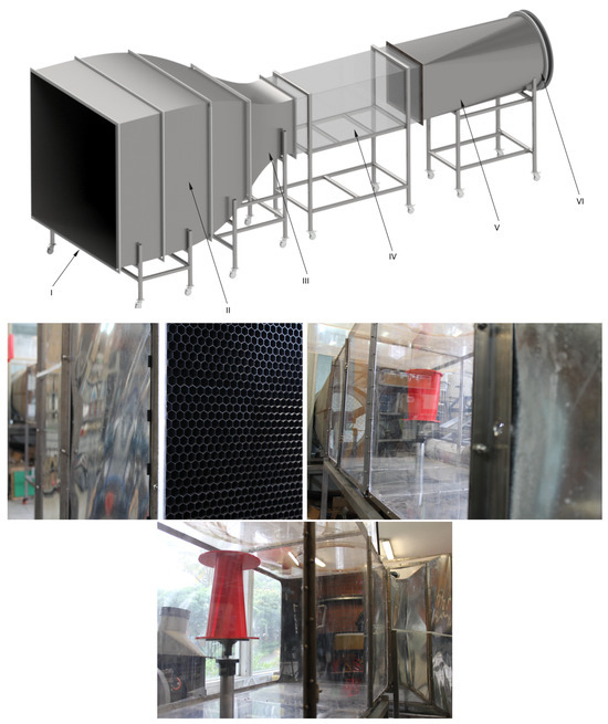
Figure 3.
Key sections of the wind tunnel and photographic views. Top: schematic representation of the main components, including intake zone (I), flow conditioning zone (II), contraction zone (III), test section (IV), diffuser (V), and power unit (VI). Bottom: photographs of the actual wind tunnel showing the intake zone and the test section.
Although wind tunnels might look a bit different depending on the design, they generally have a similar setup comprising six main parts. Each of these sections plays a critical role in ensuring that the airflow is suitable for accurate aerodynamic testing. The intake zone (I), also known as the suction zone, is where air enters the tunnel. Elements, such as honeycomb structures, are often installed to reduce turbulence, helping to maintain a uniform airflow before it proceeds to the next stage. The flow conditioning zone (II) further stabilizes the airflow using flow straighteners or screens. The goal is to eliminate irregularities and achieve a laminar, predictable flow suitable for precise measurements. The tunnel’s cross-sectional area gradually narrows in the contraction zone (III), causing a controlled increase in airflow speed. This step is crucial for achieving the required wind speed before the air reaches the test section.
The test section (IV) is the most important part of the wind tunnel. Here, the object or model under investigation is positioned. The test section has a square cross-section of 0.8 m × 0.8 m. An important consideration in wind tunnel testing is the blockage effect, which is the ratio of the model’s frontal area to the cross-sectional area of the test section. For our models, the blockage ratios were computed for each of the nine experimental runs, resulting in values of 4% (Models 1, 4, and 7), 8% (Model 2, 5, and 8), and 13% (Models 3, 6, and 9). No blockage correction was applied to the experimental data. The primary implication of this is that the measured flow velocity around the model may be artificially accelerated, leading to a slight overestimation of the turbine’s performance coefficients.
With the airflow now stabilized and accelerated, it becomes possible to accurately measure its interaction with the test model. The wind velocity in the test section was measured using a Flowatch anemometer with a 20 mm impeller, a minimum sensitivity below 1 m/s, ±2% accuracy, and an off-axis error tolerance of ±30° (±3%). This setup ensured that the airflow conditions were stable and adequately characterized for aerodynamic testing. Following the test section, the air enters the diffuser (V), where the tunnel’s cross-section gradually expands. This helps reduce energy loss and ensures a smooth exit of air.
Finally, the power unit or fan (VI) keeps the airflow moving through the tunnel. In this case, the tunnel uses a Soler Palau TGT/6-1000-9/26-B-7 1/2HP-3-208-230/460V axial tubular fan (Barcelona, Spain) with aluminum blades and a three-phase motor. This fan can pump out 15.1 m3/s at a static pressure of 27.1 Pa, ensuring a steady and suitable airflow for aerodynamic tests.
As for the data acquisition system, it features a Futek rotary torque sensor (model TRS 605-FSH02052, Irvine, CA, USA) with an integrated encoder and a 6 V DC motor rated at 300 rpm with a gear reducer. The torque sensor operates within the range of 0–1 Nm. In the setup, the DC motor acts as a braking device and is connected to a regulated power supply that allows fine control of voltage and current, thereby increasing the resistive load on the motor. This arrangement helps researchers simulate different operational loads and precisely measure the torque output of the turbine at varying rotational speeds, making it really effective for evaluating performance in wind tunnel scenarios.
2.5. Rotor Manufacturing via 3D Printing
For making the nine turbine models, 3D printing was employed using PETG filament as the printing material. Three-dimensional printing is a process where three-dimensional objects are formed by depositing material layer by layer from a digital model. It is great for making prototypes and testing out designs because it can handle complex shapes with precision and plenty of customization options. For this study, Creality brand printers were used. They are known for their reliability and ability to work with engineering-grade materials like PETG. This filament was chosen for its excellent mechanical properties, such as strength and durability, which are essential for printing turbine models [67,68]. In particular, the turbines with aspect ratios of 2 and 1.35 were printed using the Creality CR-M4 due to its larger build volume, while the turbines with an aspect ratio of 0.7 were manufactured with the Creality K1C, which has a smaller build volume better suited for these compact geometries. Table 2 presents the characteristics of the material and the specifications of the 3D printers.
Table 2.
Three-dimensional printer specifications and material properties.
The turbine models were printed in two main parts. The first section included one of the end caps and the turbine blades, along with the secondary element. The second section consisted of the other end cap, which was printed with slots or guides. These slots allow for a secure and precise fit with the first section, which ensures proper alignment and the structural integrity of the final model. The printed turbines are shown in Table 3. Although two different printers were used to accommodate the model sizes, the printing parameters were kept identical for both machines to ensure the consistency and comparability of all manufactured parts. The specific settings used were an extrusion temperature of 220 °C, a printing speed of 150 mm/s, and a bed temperature of 70 °C. Additionally, the infill percentage was set to 100% for maximum solidity, and a layer height of 0.2 mm was used. This standardized setup guaranteed that all models shared the same surface finish and internal structure, minimizing any variability from the manufacturing process. Table 2 presents the characteristics of the material and the specifications of the 3D printers.
Table 3.
Printed turbine models.
3. Results and Discussion
Figure 4 presents the performance curves, showing as a function of , enabling a direct comparison of each design’s efficiency. The maximum values for each model are summarized in Table 4. Experiments were conducted using the test models in the wind tunnel described in previous sections, with the aim of evaluating their aerodynamic performance. During testing, velocities varied from 5 to 10 m/s, ensuring representative conditions for analyzing the operational behavior of the models. It is important to clarify that while multiple runs were conducted for each model to validate the consistency of the results, the curves shown in this figure represent the single, most representative run for each design. As this approach uses single-run data for the final analysis, this is noted as a limitation. In the figure, the scattered markers represent the experimental measurements, while the continuous curves correspond to the fitted trend lines, allowing for a clearer visualization of the performance tendencies of each model.
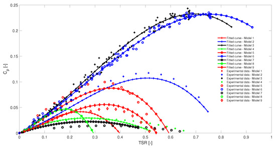
Figure 4.
Performance curves of the Savonius rotor models: as a function of .
Table 4.
Experimental results and model predictions.
Based on the maximum values obtained from each performance curve, RSM was used to optimize the design of the models. To obtain a statistically reliable regression model, was transformed using the natural logarithm function. Without the transformation or trying other options like the square root, cube root, or logarithm, the model failed to meet the significance threshold (p < 0.05), which undermined its validity.
The natural logarithm transformation proved effective in stabilizing variance, improving the normality of residuals, and reducing heteroscedasticity. The choice of transformation was determined through an iterative testing process aimed at optimizing both the goodness of fit and the statistical significance of the model coefficients. Although other transformations were explored, only the natural logarithm yielded a model with meaningful explanatory power, ensuring that the model’s significance is crucial as it validates the reliability of the observed relationships between the design parameters and the turbine’s aerodynamic performance.
The initial regression model included one independent factor, two linear terms, two quadratic terms, and one interaction term, as in Equation (5). However, after evaluating the statistical contribution of each term, the quadratic factor associated with the aspect ratio () was removed, resulting in a reduced model that maintained significance. Further statistical tests, such as residual analysis and model adequacy checks, will be presented later in the text to verify the validity of the final regression model. The resulting reduced model, based on the transformed response variable, is expressed in Equation (9).
Table 4 presents the transformed values, the values predicted by the regression model, and the residuals, which are the differences between the experimental and predicted values. An ANOVA test was also performed to evaluate the impact of the factors on . The results are presented in Table 5.
Table 5.
ANOVA results.
The regression model has a p-value of 0.005652, revealing that it is statistically significant at a confidence level above 95%. This means that at least one of the factors included in the model has a real effect on the response variable. The coefficient is 0.9559, which means the model explains 95.59% of the observed variability in the data. Furthermore, the adjusted , which accounts for the inclusion of irrelevant variables, is 0.9119. This demonstrates that the model retains a good fit without overfitting, confirming its robustness. These values reflect the model’s quality and its capacity to adequately describe the relationship between , , and .
According to Table 5, the factor has a statistically significant effect on (p-value = 0.00922), indicating that variations in this factor meaningfully influence the model’s behavior. Its high F-value (22.209) has a strong impact. The factor is even more significant (p-value = 0.00154), demonstrating a greater influence on the response variable than .
Its sum of squares is more than twice that of , and its high F-value (59.167) indicates that the variability explained by is substantially greater than the variability due to error. On the other hand, the quadratic term of is not statistically significant (p > 0.05), suggesting that it does not contribute meaningfully to the model’s variability. This implies that the relationship between and the response variable is likely linear, without notable curvature. The interaction effect between and is also not significant (p > 0.05), recommending that the factors operate independently, without significantly influencing each other in their effect on the response.
For a regression model to be effective and ready for optimization, there are a few key assumptions that need to be in check, alongside significance: normality, independence, and constant variance (which we call homoscedasticity) of the residuals. Residual normality ensures that the errors follow an approximately normal distribution, enabling reliable statistical inference about the model coefficients. This assumption can be tested using procedures such as the Jarque–Bera and Shapiro–Wilk tests. Error independence means there is no correlation among residuals, which is essential to avoid biased parameter estimation and can be examined using the Durbin–Watson test. Homoscedasticity implies that the variance of residuals remains constant across the range of predictor values, which is crucial to maintaining the accuracy of the model’s predictions. Tests such as Breusch–Pagan or White can be used to assess this assumption. If any of these assumptions are off, the model’s estimates could be inefficient, which might undermine its usefulness for optimization and making decisions.
Figure 5 and Table 6 present the results of various normality tests, which cover both graphical and numerical aspects such as p-values and F-statistics. The graphical representations include a frequency histogram (Figure 5b) and a quantile–quantile (QQ) plot (Figure 5a). Normality can be initially evaluated by visually inspecting the histogram, where the residuals distribution appears approximately symmetric and bell-shaped, consistent with a normal distribution. The QQ plot further supports this observation as most data points align closely with the reference diagonal line, with only minor deviations at the tails. This alignment indicates that the residuals follow the normality assumption reasonably well. Complementing these graphical tools, the statistical tests in Table 6 provide a quantitative assessment, confirming normality when the p-value is greater than 0.05. Together, these results suggest that the residuals meet the assumptions of normality, thereby validating the adequacy of the regression model used in this study.
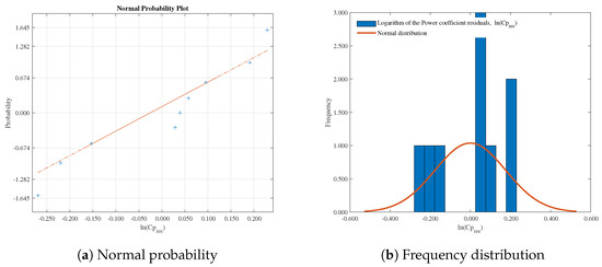
Figure 5.
Normality test of the logarithmic power coefficient residuals (): (a) normal probability and (b) frequency distribution of residuals compared with the fitted normal curve.
Table 6.
Normality test results.
To validate the independence of the residuals, the Durbin–Watson test was applied, yielding a p-value of 0.1329. This indicates no significant evidence of autocorrelation among the residuals. Additionally, to assess homoscedasticity, the Breusch–Pagan test was performed, resulting in a p-value of 0.5269. This suggests that the residuals exhibit constant variance. Based on these results, the regression model is considered statistically valid, and the optimization process can proceed.
Finally, Figure 6 shows the resulting response surface and contour plot, which illustrate the relationship between the model variables and enable identification of the optimal point within the design space.
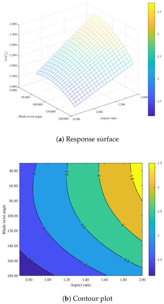
Figure 6.
Response surface and contour plots showing the effect of blade twist angle and aspect ratio on the logarithm of the power coefficiernt ().
From Figure 6, it can be observed that values tend to increase toward the upper right region of the plots, where the aspect ratio is higher (close to 2.0) and the blade twist angle is lower (around 30–40°). Conversely, the lowest values are in the lower left region, corresponding to a lower aspect ratio (0.8) and higher twist angles (around 180°). Since the goal is to maximize , the optimal point lies in the region with the highest values.
Once the region where and maximize is identified, Equation (9) is applied to determine the combination of and values that yield the highest . This process may result in combinations different from those tested in the initial design of experiments presented in Table 1. In the case of , since the response variable was transformed using the natural logarithm, the regression model predicts values of rather than directly. Therefore, once the optimal values of the independent variables (in this case, and ) are determined from the model, the corresponding value must be converted back to the original scale by applying the inverse transformation, i.e., the exponential function. According to the Equation (9) analysis, this corresponds to an aspect ratio () of approximately 2.0 and a twist angle () close to 30°. The optimal configuration matches one of the initial designs in the experimental matrix, specifically, model 3, which features a twist angle of 30° and an aspect ratio of 2.0. For this configuration, the experimentally obtained value was 0.2326.
Although this value is comparable to the range reported in the literature (typically 0.20–0.25) [29,30], direct comparisons should be made with caution. Previous works often relied on specific blade profiles that were optimized under particular flow conditions, whereas the present study focuses on a novel multielement blade configuration. Consequently, differences in the blade geometry, Reynolds number, and overlap ratio contribute to variations in the reported values.
From the results, a lower can improve aerodynamic efficiency by maintaining a more uniform angle of attack along the blade span. Excessive twist can lead to sections of the blade operating at suboptimal angles, causing premature flow separation and a reduction in the lift-to-drag ratio. A lower twist angle promotes a more consistent pressure distribution, which enhances energy capture and reduces aerodynamic losses, especially under uniform inflow conditions typical of controlled wind tunnel experiments. Refs. [50,54] used twist angles of 0°, 45°, 90°, 135°, and 180° and found that the maximum was achieved at a of 45°, with a value of 0.13 and 0.22, respectively. This result supports the conclusion of the present study that improvements are obtained for low twist angles. It is worth noting that these authors did not modify the aspect ratio in their analysis.
From a manufacturing and structural perspective, blades with a lower twist angle are easier to fabricate and assemble with high dimensional accuracy. High twist geometries often require complex molds or multi-step manufacturing processes, which increase production costs and the potential for defects. Moreover, reduced twist angles result in simpler load paths within the blade structure, improving stiffness-to-weight ratios and minimizing structural stress concentrations, thereby increasing durability and reliability over long-term operation.
A higher contributes to improved performance primarily by increasing the rotor’s swept area for a given chord length, which directly enhances the potential energy capture from the wind. Physically, a high reduces induced drag by lowering the strength of tip vortices, leading to higher aerodynamic efficiency [69]. From a design perspective, an increased allows for a larger effective rotor diameter without excessively increasing blade chord, thus optimizing both aerodynamic and structural performance while maintaining material efficiency.
The novelty of the present work lies not solely in achieving comparable efficiency but in the methodology employed. By applying a full factorial response surface design, we systematically explored a broader parameter space than typically considered, identifying both upper and lower performance bounds associated with and . This approach not only confirms the viability of the proposed configuration but also provides a framework that can be extended to include additional design variables to potentially achieve higher values in future optimizations.
Because both and are dimensionless parameters, the optimized configurations identified in this study can be scaled to larger rotor sizes without losing their aerodynamic relevance. This implies that the proposed designs could be adapted for urban or distributed generation scenarios, where compact and efficient vertical-axis turbines are of particular interest. Moreover, the designed turbine and small-scale vertical-axis wind turbines in general are particularly well suited for distributed generation and off-grid electrification since they can be installed close to the point of consumption, require less space, and operate efficiently under multidirectional and turbulent wind conditions. As such, they represent a promising technology to complement other renewable sources, reduce dependence on centralized power grids, and contribute to the ongoing energy transition toward cleaner and more sustainable systems. However, while the present results are based on controlled laboratory conditions, real-world operation involves variable wind speeds, turbulence intensity, and inflow angles that may influence performance. Therefore, field testing under urban or turbulent environments will be essential to validate the scalability of the optimized designs and to fully assess their long-term energy capture potential.
4. Conclusions
Savonius wind turbines represent a prospective solution for energy generation, particularly in low-wind-speed environments. Their simple geometry, one-directional operation, and robust design make them attractive for small-scale and urban applications where conventional horizontal-axis wind turbines may not be viable. However, the relatively low aerodynamic efficiency of Savonius rotors necessitates careful geometric optimization to improve their power coefficient () and ensure their competitiveness as a renewable energy technology.
The experimental results obtained in this study confirm that the blade twist angle () and the aspect ratio () are decisive parameters in determining the aerodynamic performance of Savonius rotors. Analysis of the response surfaces revealed that higher values (close to 2.0) combined with lower twist angles (30–40°) yield the highest , whereas low and high values result in significantly poorer performance. Through an optimization procedure, we identified the optimal configuration as an of 2.0 and a of 30°, which corresponds to model 3 in the experimental design. Under these conditions, the turbine achieved an experimentally measured power coefficient of .
To better illustrate the practical significance of this result, it can be translated into real-world power output. Since the extractable power from the wind is directly proportional to both and the cube of the wind speed, even modest increases in efficiency have a substantial impact. For example, at the optimized , the turbine would deliver around 15–20% more power than a configuration with under the same wind conditions. Likewise, an increase in the average wind speed from 5 m/s to 7 m/s would nearly triple the output, underscoring the sensitivity of energy capture to both aerodynamic efficiency and environmental conditions. These comparisons confirm that the optimized design is competitive with benchmarks reported in the literature and highlight its tangible potential for distributed generation and off-grid applications.
The results highlight that reducing the twist angle improves aerodynamic efficiency by maintaining a more uniform angle of attack along the blade span, thereby reducing premature flow separation and aerodynamic losses. From a structural and manufacturing standpoint, low-twist blades are also easier to fabricate, less costly, and mechanically more reliable. Similarly, making the aspect ratio larger increases the area and reduces induced drag, leading to higher aerodynamic efficiency while also offering structural benefits such as improved stiffness-to-weight ratios.
This study shows that using geometric optimization with factorial design and response surface methodology is a solid way to boost the performance of Savonius vertical-axis wind turbines (VAWTs). The identification of an optimal configuration with confirms the potential of carefully tuned blade geometry to enhance aerodynamic efficiency, structural simplicity, and durability. These results highlight the potential of Savonius rotors as a great option for small-scale wind energy collection, especially in areas with low wind speeds.
With the optimal model identified, the next step is to design it at a relevant scale for real-world implementation. This process will involve adapting the rotor to a suitable size for practical applications, along with integrating the additional mechanical components necessary for field operation. These components include the power transmission system, the electrical generator, and the supporting structure, all of which will ensure efficient and stable turbine performance under real operating conditions. This development will allow for the evaluation of the turbine’s performance in practical settings and support the advancement of its viability for renewable energy generation.
Author Contributions
Conceptualization, J.R., A.S., L.V., A.R.-C. and E.C.; methodology, L.V., J.R., A.S. and E.C.; software, A.S. and L.V.; validation, A.S., L.V. and J.R.; formal analysis, L.V. and E.C.; writing—original draft, L.V., A.R.-C. and E.C.; writing—review and editing, A.R.-C. and E.C.; supervision, E.C.; project administration, A.R.-C. and E.C.; funding acquisition, E.C. All authors have read and agreed to the published version of the manuscript.
Funding
The authors gratefully acknowledge the financial support provided by the Colombian Ministry of Science, Technology, and Innovation “MinCiencias” through “Patrimonio Autónomo Fondo Nacional de Financiamiento para la Ciencia, la Tecnología y la Innovación, Francisco José de Caldas” (Perseo Alliance, Contract No. 112721-392-2023).
Data Availability Statement
The original contributions presented in the study are included in the article; further inquiries can be directed to the corresponding author.
Conflicts of Interest
The authors declare no conflicts of interest.
References
- Newman, P.; Beatley, T.; Boyer, H. Resilient Cities: Overcoming Fossil Fuel Dependence; Island Press: Washington, DC, USA, 2017. [Google Scholar]
- Mayer, A. Fossil fuel dependence and energy insecurity. Energy Sustain. Soc. 2022, 12, 27. [Google Scholar] [CrossRef]
- Backhouse, M.; Rodríguez, F.; Tittor, A. From a Fossil Towards a Renewable Energy Regime in the Americas? Socio-Ecological Inequalities, Contradictions and Challenges for a Global Bioeconomy; Friedrich-Schiller-University: Jena, Germany, 2019. [Google Scholar]
- Saleh, H.M.; Hassan, A.I. The challenges of sustainable energy transition: A focus on renewable energy. Appl. Chem. Eng. 2024, 7, 2084. [Google Scholar] [CrossRef]
- Balakrishnan, P. Global Renewable Energy Transition Challenges and Strategic Solutions. In Geopolitical Landscapes of Renewable Energy and Urban Growth; IGI Global Scientific Publishing: Hershey, PA, USA, 2025; pp. 63–96. [Google Scholar]
- Adewumi, A.; Olu-lawal, K.A.; Okoli, C.E.; Usman, F.O.; Usiagu, G.S. Sustainable energy solutions and climate change: A policy review of emerging trends and global responses. World J. Adv. Res. Rev. 2024, 21, 408–420. [Google Scholar]
- Kumar, A. Global warming, climate change and greenhouse gas mitigation. In Biofuels: Greenhouse Gas Mitigation and Global Warming: Next Generation Biofuels and Role of Biotechnology; Springer: Berlin/Heidelberg, Germany, 2018; pp. 1–16. [Google Scholar]
- Singh, S. Energy crisis and climate change: Global concerns and their solutions. In Energy: Crises, Challenges and Solutions; John Wiley & Sons: Hoboken, NJ, USA, 2021; pp. 1–17. [Google Scholar]
- Kumar, S.; Rathore, K. Renewable energy for sustainable development goal of clean and affordable energy. Int. J. Mater. Manuf. Sustain. Technol. 2023, 2, 1–15. [Google Scholar] [CrossRef]
- Firoozi, A.A.; Firoozi, A.A.; Hejazi, F. Innovations in wind turbine blade engineering: Exploring materials, sustainability, and market dynamics. Sustainability 2024, 16, 8564. [Google Scholar] [CrossRef]
- Firoozi, A.A.; Hejazi, F.; Firoozi, A.A. Advancing wind energy efficiency: A systematic review of aerodynamic optimization in wind turbine blade design. Energies 2024, 17, 2919. [Google Scholar] [CrossRef]
- Afridi, S.K.; Koondhar, M.A.; Jamali, M.I.; Alaas, Z.M.; Alsharif, M.H.; Kim, M.K.; Mahariq, I.; Touti, E.; Aoudia, M.; Ahmed, M. Winds of progress: An in-depth exploration of offshore, floating, and onshore wind turbines as cornerstones for sustainable energy generation and environmental stewardship. IEEE Access 2024, 12, 66147–66166. [Google Scholar] [CrossRef]
- Simoes, M.G.; Farret, F.A.; Khajeh, H.; Shahparasti, M.; Laaksonen, H. Future renewable energy communities based flexible power systems. Appl. Sci. 2021, 12, 121. [Google Scholar] [CrossRef]
- Cai, Y.; Bréon, F.M. Wind power potential and intermittency issues in the context of climate change. Energy Convers. Manag. 2021, 240, 114276. [Google Scholar] [CrossRef]
- Teff-Seker, Y.; Berger-Tal, O.; Lehnardt, Y.; Teschner, N. Noise pollution from wind turbines and its effects on wildlife: A cross-national analysis of current policies and planning regulations. Renew. Sustain. Energy Rev. 2022, 168, 112801. [Google Scholar] [CrossRef]
- Nazir, M.S.; Ali, N.; Bilal, M.; Iqbal, H.M. Potential environmental impacts of wind energy development: A global perspective. Curr. Opin. Environ. Sci. Health 2020, 13, 85–90. [Google Scholar] [CrossRef]
- Rinaldi, G.; Thies, P.R.; Johanning, L. Current status and future trends in the operation and maintenance of offshore wind turbines: A review. Energies 2021, 14, 2484. [Google Scholar] [CrossRef]
- Shields, M.; Beiter, P.; Nunemaker, J.; Cooperman, A.; Duffy, P. Impacts of turbine and plant upsizing on the levelized cost of energy for offshore wind. Appl. Energy 2021, 298, 117189. [Google Scholar] [CrossRef]
- Das, A.; Chimonyo, K.B.; Kumar, T.R.; Gourishankar, S.; Rani, C. Vertical axis and horizontal axis wind turbine-A comprehensive review. In Proceedings of the 2017 International Conference on Energy, Communication, Data Analytics and Soft Computing (ICECDS), Chennai, India, 1–2 August 2017; pp. 2660–2669. [Google Scholar]
- Johari, M.K.; Jalil, M.; Shariff, M.F.M. Comparison of horizontal axis wind turbine (HAWT) and vertical axis wind turbine (VAWT). Int. J. Eng. Technol. 2018, 7, 74–80. [Google Scholar] [CrossRef]
- Al-Rawajfeh, M.A.; Gomaa, M.R. Comparison between horizontal and vertical axis wind turbine. Int. J. Appl. Power Eng. 2023, 12, 13–23. [Google Scholar] [CrossRef]
- Kumar, R.; Raahemifar, K.; Fung, A.S. A critical review of vertical axis wind turbines for urban applications. Renew. Sustain. Energy Rev. 2018, 89, 281–291. [Google Scholar] [CrossRef]
- Liu, J.; Lin, H.; Zhang, J. Review on the technical perspectives and commercial viability of vertical axis wind turbines. Ocean Eng. 2019, 182, 608–626. [Google Scholar] [CrossRef]
- Ahmad, M.; Shahzad, A.; Qadri, M.N.M. An overview of aerodynamic performance analysis of vertical axis wind turbines. Energy Environ. 2023, 34, 2815–2857. [Google Scholar] [CrossRef]
- Roy, S.; Saha, U.K. Review on the numerical investigations into the design and development of Savonius wind rotors. Renew. Sustain. Energy Rev. 2013, 24, 73–83. [Google Scholar] [CrossRef]
- Anbarsooz, M. Aerodynamic performance of helical Savonius wind rotors with 30 and 45 twist angles: Experimental and numerical studies. Proc. Inst. Mech. Eng. Part A J. Power Energy 2016, 230, 523–534. [Google Scholar] [CrossRef]
- Kothe, L.B.; Möller, S.V.; Petry, A.P. Numerical and experimental study of a helical Savonius wind turbine and a comparison with a two-stage Savonius turbine. Renew. Energy 2020, 148, 627–638. [Google Scholar] [CrossRef]
- Jeon, K.S.; Jeong, J.I.; Pan, J.K.; Ryu, K.W. Effects of end plates with various shapes and sizes on helical Savonius wind turbines. Renew. Energy 2015, 79, 167–176. [Google Scholar] [CrossRef]
- Zadeh, M.N.; Pourfallah, M.; Sabet, S.S.; Gholinia, M.; Mouloodi, S.; Ahangar, A.T. Performance assessment and optimization of a helical Savonius wind turbine by modifying the Bach’s section. SN Appl. Sci. 2021, 3, 739. [Google Scholar] [CrossRef]
- Damak, A.; Driss, Z.; Abid, M. Optimization of the helical Savonius rotor through wind tunnel experiments. J. Wind Eng. Ind. Aerodyn. 2018, 174, 80–93. [Google Scholar] [CrossRef]
- Kamoji, M.; Kedare, S.B.; Prabhu, S. Performance tests on helical Savonius rotors. Renew. Energy 2009, 34, 521–529. [Google Scholar] [CrossRef]
- Lajnef, M.; Mosbahi, M.; Abid, H.; Driss, Z.; Amato, E.; Picone, C.; Sinagra, M.; Tucciarelli, T. Numerical and experimental investigation for helical savonius rotor performance improvement using novel blade shapes. Ocean Eng. 2024, 309, 118357. [Google Scholar] [CrossRef]
- Lajnef, M.; Mosbahi, M.; Chouaibi, Y.; Driss, Z. Performance improvement in a helical Savonius wind rotor. Arab. J. Sci. Eng. 2020, 45, 9305–9323. [Google Scholar] [CrossRef]
- Damak, A.; Driss, Z.; Abid, M.S. Experimental investigation of helical Savonius rotor with a twist of 180. Renew. Energy 2013, 52, 136–142. [Google Scholar] [CrossRef]
- Rosato, A.; Perrotta, A.; Maffei, L. Commercial small-scale horizontal and vertical wind turbines: A comprehensive review of geometry, materials, costs and performance. Energies 2024, 17, 3125. [Google Scholar] [CrossRef]
- Chaudhuri, A.; Datta, R.; Kumar, M.P.; Davim, J.P.; Pramanik, S. Energy conversion strategies for wind energy system: Electrical, mechanical and material aspects. Materials 2022, 15, 1232. [Google Scholar] [CrossRef]
- Bello, S.F.; Lawal, R.O.; Ige, O.B.; Adebayo, S.A. Optimizing vertical axis wind turbines for urban environments: Overcoming design challenges and maximizing efficiency in low-wind conditions. GSC Adv. Res. Rev. 2024, 21, 246–256. [Google Scholar] [CrossRef]
- Micallef, D.; Van Bussel, G. A review of urban wind energy research: Aerodynamics and other challenges. Energies 2018, 11, 2204. [Google Scholar] [CrossRef]
- Dewan, A.; Gautam, A.; Goyal, R. Savonius wind turbines: A review of recent advances in design and performance enhancements. Mater. Today Proc. 2021, 47, 2976–2983. [Google Scholar] [CrossRef]
- Laws, P.; Saini, J.S.; Kumar, A.; Mitra, S. Improvement in Savonius wind turbines efficiency by modification of blade designs—A numerical study. J. Energy Resour. Technol. 2020, 142, 061303. [Google Scholar] [CrossRef]
- Alom, N.; Saha, U.K. Evolution and progress in the development of savonius wind turbine rotor blade profiles and shapes. J. Sol. Energy Eng. 2019, 141, 030801. [Google Scholar] [CrossRef]
- Chen, L.; Chen, J.; Zhang, Z. Review of the Savonius rotor’s blade profile and its performance. J. Renew. Sustain. Energy 2018, 10, 013306. [Google Scholar] [CrossRef]
- Talukdar, P.K.; Kulkarni, V.; Saha, U.K. Performance estimation of Savonius wind and Savonius hydrokinetic turbines under identical power input. J. Renew. Sustain. Energy 2018, 10, 064704. [Google Scholar] [CrossRef]
- Alom, N.; Saha, U.K.; Dewan, A. In the quest of an appropriate turbulence model for analyzing the aerodynamics of a conventional Savonius (S-type) wind rotor. J. Renew. Sustain. Energy 2021, 13, 023313. [Google Scholar] [CrossRef]
- Gallo, L.A.; Chica, E.L.; Flórez, E.G. Numerical optimization of the blade profile of a savonius type rotor using the response surface methodology. Sustainability 2022, 14, 5596. [Google Scholar] [CrossRef]
- Saeed, H.A.H.; Elmekawy, A.M.N.; Kassab, S.Z. Numerical study of improving Savonius turbine power coefficient by various blade shapes. Alex. Eng. J. 2019, 58, 429–441. [Google Scholar] [CrossRef]
- Gallo, L.A.; Chica, E.L.; Flórez, E.G.; Obando, F.A. Numerical and experimental study of the blade profile of a Savonius type rotor implementing a multi-blade geometry. Appl. Sci. 2021, 11, 10580. [Google Scholar] [CrossRef]
- Peng, H.; Lam, H.; Liu, H. Power performance assessment of H-rotor vertical axis wind turbines with different aspect ratios in turbulent flows via experiments. Energy 2019, 173, 121–132. [Google Scholar] [CrossRef]
- Shamsoddin, S.; Porté-Agel, F. Effect of aspect ratio on vertical-axis wind turbine wakes. J. Fluid Mech. 2020, 889, R1. [Google Scholar] [CrossRef]
- El-Askary, W.; Saad, A.S.; AbdelSalam, A.M.; Sakr, I. Investigating the performance of a twisted modified Savonius rotor. J. Wind Eng. Ind. Aerodyn. 2018, 182, 344–355. [Google Scholar] [CrossRef]
- Zakaria, A.; Ibrahim, M. Effect of twist angle on starting capability of a Savonius rotor–CFD analysis. IOP Conf. Ser. Mater. Sci. Eng. 2020, 715, 012014. [Google Scholar] [CrossRef]
- Anderson, V.L.; McLean, R.A. Design of Experiments: A Realistic Approach; CRC Press: Boca Raton, FL, USA, 2018. [Google Scholar]
- Jankovic, A.; Chaudhary, G.; Goia, F. Designing the design of experiments (DOE)—An investigation on the influence of different factorial designs on the characterization of complex systems. Energy Build. 2021, 250, 111298. [Google Scholar] [CrossRef]
- Lee, J.H.; Lee, Y.T.; Lim, H.C. Effect of twist angle on the performance of Savonius wind turbine. Renew. Energy 2016, 89, 231–244. [Google Scholar] [CrossRef]
- Farozan, I.; Soelaiman, T.A.F.; Soetikno, P.; Indartono, Y.S. The effect of rotor aspect ratio, stages, and twist angle on Savonius wind turbine performance in low wind speeds environment. Results Eng. 2025, 25, 104041. [Google Scholar] [CrossRef]
- Bouvant, M.; Betancour, J.; Velásquez, L.; Rubio-Clemente, A.; Chica, E. Design optimization of an Archimedes screw turbine for hydrokinetic applications using the response surface methodology. Renew. Energy 2021, 172, 941–954. [Google Scholar] [CrossRef]
- Romero-Menco, F.; Betancour, J.; Velásquez, L.; Rubio-Clemente, A.; Chica, E. Horizontal-axis propeller hydrokinetic turbine optimization by using the response surface methodology: Performance effect of rake and skew angles. Ain Shams Eng. J. 2024, 15, 102596. [Google Scholar] [CrossRef]
- Fox, J. Regression Diagnostics: An Introduction; Sage Publications: Thousand Oaks, CA, USA, 2019. [Google Scholar]
- Montgomery, D.C.; Peck, E.A.; Vining, G.G. Introduction to Linear Regression Analysis; John Wiley & Sons: Hoboken, NJ, USA, 2021. [Google Scholar]
- Fraiman, D.; Fraiman, R. An ANOVA approach for statistical comparisons of brain networks. Sci. Rep. 2018, 8, 4746. [Google Scholar] [CrossRef]
- Potvin, C. ANOVA: Experiments in controlled environments. In Design and Analysis of Ecological Experiments; Chapman and Hall/CRC: Hoboken, NJ, USA, 2020; pp. 46–68. [Google Scholar]
- Ware, J.H.; Mosteller, F.; Delgado, F.; Donnelly, C.; Ingelfinger, J.A. P values. In Medical Uses of Statistics; CRC Press: Hoboken, NJ, USA, 2019; pp. 181–200. [Google Scholar]
- Di Leo, G.; Sardanelli, F. Statistical significance: P value, 0.05 threshold, and applications to radiomics—Reasons for a conservative approach. Eur. Radiol. Exp. 2020, 4, 18. [Google Scholar] [CrossRef]
- Saada, K.; Amroune, S.; Zaoui, M. Prediction of mechanical behavior of epoxy polymer using Artificial Neural Networks (ANN) and Response Surface Methodology (RSM). Fract. Struct. Integr. 2023, 17, 191–206. [Google Scholar] [CrossRef]
- Prabhahar, M.; Athitya, M.P.; Chitrambalam, M.T.; Prabhu, L.; Prakash, S. Experimental investigation of MS material in laser cutting machine using Taguchi method. AIP Conf. Proc. 2022, 2426, 020019. [Google Scholar] [CrossRef]
- Zhang, W. p-value based statistical significance tests: Concepts, misuses, critiques, solutions and beyond. Comput. Ecol. Softw. 2022, 12, 80. [Google Scholar]
- Valvez, S.; Silva, A.P.; Reis, P.N. Optimization of printing parameters to maximize the mechanical properties of 3D-printed PETG-based parts. Polymers 2022, 14, 2564. [Google Scholar] [CrossRef] [PubMed]
- Hsueh, M.H.; Lai, C.J.; Wang, S.H.; Zeng, Y.S.; Hsieh, C.H.; Pan, C.Y.; Huang, W.C. Effect of printing parameters on the thermal and mechanical properties of 3D-printed pla and petg, using fused deposition modeling. Polymers 2021, 13, 1758. [Google Scholar] [CrossRef] [PubMed]
- Prabowoputra, D.M.; Prabowo, A.R. Effect of geometry modification on turbine performance: Mini-review of Savonius rotor. Int. J. Mech. Eng. Robot. Res. 2022, 11, 777–783. [Google Scholar] [CrossRef]


Disclaimer/Publisher’s Note: The statements, opinions and data contained in all publications are solely those of the individual author(s) and contributor(s) and not of MDPI and/or the editor(s). MDPI and/or the editor(s) disclaim responsibility for any injury to people or property resulting from any ideas, methods, instructions or products referred to in the content. |
© 2025 by the authors. Licensee MDPI, Basel, Switzerland. This article is an open access article distributed under the terms and conditions of the Creative Commons Attribution (CC BY) license (https://creativecommons.org/licenses/by/4.0/).