Smart Energy Strategy for AC Microgrids to Enhance Economic Performance in Grid-Connected and Standalone Operations: A Gray Wolf Optimizer Approach

Abstract

This study proposes an optimized energy management strategy for alternating current microgrids, integrating wind generation, battery energy storage systems (BESSs), and distribution static synchronous compensators (D-STATCOMs). The objective is to minimize operational costs, including grid electricity purchases (grid-connected mode), diesel generation costs (islanded mode), and maintenance expenses of distributed energy resources while ensuring voltage limits, maximum line currents, and power balance. A master–slave optimization approach is employed, where the Gray Wolf Optimizer (GWO) determines the optimal dispatch of energy resources, and successive approximations (SAs) perform power flow analysis. The methodology was validated on a 33-node microgrid, considering variable wind generation and demand profiles from a Colombian region under grid-connected and islanded conditions. To assess performance, 100 independent runs per method were conducted, comparing GWO against particle swarm optimization (PSO) and genetic algorithms (GAs). Statistical analysis confirmed that GWO achieved the lowest operational costs (USD 3299.39 in grid-connected mode and USD 11,367.76 in islanded mode), the highest solution stability (0.19% standard deviation), and superior voltage regulation. The results demonstrate that GWO with SA provides the best trade-off between cost efficiency, system stability, and computational performance, making it an optimal approach for microgrid energy management.

1. Introduction

1.1. Problem Description

The increasing complexity of electrical networks—driven by rising energy demand, renewable energy penetration, and evolving grid architectures—necessitates innovative solutions for optimal energy management. A critical challenge is the efficient coordination of multiple distributed energy resources (DERs) operating under both grid-connected (on-grid) and islanded conditions (off-grid), ensuring technical feasibility, cost-effectiveness, and grid stability. This study focuses on optimizing the joint operation of wind generators, battery energy storage systems (BESSs), and distribution static synchronous compensators (D-STATCOMs) within AC microgrids, a problem that remains underexplored in the literature.

The development of humanity and the rapid increase in population have created the need to propose new methods for supplying and managing electrical grids [1]. In this context, microgrids have emerged as a practical solution, integrating renewable energy sources, static reactive compensators, battery energy storage systems, and loads [2]. These systems utilize innovative operation methodologies to optimize the use of energy resources, improving the technical and economic conditions for both users and grid operators.

Energy management in microgrids (MGs) is a highly complex nonlinear optimization problem that is critical in the transition toward more efficient and sustainable power systems [3]. The increasing integration of renewable energy sources, such as solar and wind power, introduces significant challenges related to their variability, stability, and optimal resource allocation [4]. Traditional power systems were designed for centralized generation, making it difficult to incorporate DERs without advanced management strategies. In this context, microgrids emerge as a viable solution by integrating distributed generation (DG), BESSs, and D-STATCOMs. However, their efficient operation requires sophisticated optimization methodologies capable of delivering high performance in terms of solution accuracy, repeatability, and computational efficiency [5]. The main objective is to determine the optimal scheduling of distributed energy resources over a given planning horizon, maximizing their impact on technical, economic, and environmental indicators while ensuring grid reliability and resilience.

Recent contributions have presented the relevance of hybrid AC/DC microgrid architectures in enhancing EV integration and grid operation, especially in space-constrained urban areas. For example, Yu et al. [6] introduced a scalable and cost-effective reconstruction strategy enhancing existing infrastructure to enable a 297% improvement in EV penetration while maintaining voltage stability. Further advancements by the same group in [7] proposed a hierarchical V2G dispatching strategy for fast-charging stations, showing remarkable results in peak shaving and valley filling, demonstrating the applicability of coordinated control schemes in low-voltage urban grids.

This challenge supports international and national initiatives such as the Paris Agreement [8], the sustainable development goals (SDG 7 and SDG 13) [9]. Colombia’s National Energy Plan 2050 [10], all of which promote renewable energy adoption, grid flexibility, and reduced fossil fuel dependence. Effective microgrid management helps achieve these goals by enhancing energy security, reducing operational costs, and minimizing environmental impact.

The success of these strategies depends on the ability of microgrids to balance technical reliability, economic feasibility, and environmental sustainability [11]. To ensure this balance, different key performance indicators must be evaluated: technical aspects, such as voltage stability and system resilience; economic factors, including operational cost reduction and participation in energy markets; and environmental benefits, such as the reduction of CO₂ emissions and the maximum utilization of available renewable resources [12]. A purely technical approach may not be economically viable, while an exclusively cost-driven perspective might compromise grid stability. Therefore, a comprehensive optimization strategy is required to effectively manage DGs, BESS, and D-STATCOMs within the microgrid.

While several studies have proposed optimization models for individual DERs or limited subsets, there remains a significant gap in holistic frameworks that integrate multiple DER types within a single optimization problem. Moreover, many existing models simplify the problem by assuming static demand or excluding reactive power management, limiting their practical applicability. Our study addresses these gaps by presenting an integrated optimization framework that simultaneously manages wind generation, battery storage, and D-STATCOMs, enhancing both economic and technical microgrid performance.

This research contributes to developing intelligent energy management systems, ensuring that renewable energy sources, storage solutions, and reactive power compensation devices operate optimally. Such advancements support the modernization of power grids, enhance the reliability of renewable energy systems, and align with global and national policies to achieve a sustainable energy future.

1.2. State of the Art

This section analyzes energy management strategies in AC microgrids, organized into the following four thematic categories: cost minimization, voltage regulation, holistic DER coordination, and advances in optimization techniques. This structured organization enhances comparative clarity and highlights specific research gaps.

1.2.1. Cost Minimization Strategies

Torkanga et al. [13] proposed a GA-based optimization model for efficient energy management of renewable-based DERs in AC microgrids, including wind turbines, PV systems, and BESS. Their approach simulates multi-sectoral demand while ensuring operation within technical constraints. Although successful in minimizing energy costs and emissions, the study lacks benchmarking against other metaheuristics, limiting insights into algorithmic performance.

An enhanced PSO technique was applied by the authors of [14] to operate DERs within a 33-node microgrid, aiming at operational cost and power loss reductions. While improvements in voltage profiles are reported, the absence of a comparative framework and neglect of reactive power support considerations reduce the generalizability of the results.

Leonori et al. [15] combined fuzzy logic with a genetic algorithm to enable real-time energy management decisions, focusing on balancing grid trading and ESS utilization. Despite achieving effective cost and profit optimization, the lack of integrated reactive power control coordination constrains the technical completeness of their model.

1.2.2. Voltage Regulation and Reactive Power Control

Babu et al. [16] developed an intelligent energy management system incorporating forecasting-based multi-objective optimization with genetic algorithms. Their model integrates energy storage with solar PV and wind generation, considering grid consumption and battery degradation costs, while a fuzzy decision-making strategy selects compromise solutions. Although the framework effectively addresses renewable integration and cost-degradation trade-offs, it does not explicitly manage reactive power or network constraints such as voltage and line currents.

Ref. [17] focused on voltage profile improvements and active power loss minimization through the optimal placement of D-STATCOMs and PV systems. However, the assumption of constant demand diminishes its applicability to real-world dynamic conditions.

In a dynamic simulation-based study, Ref. [18] evaluated the effectiveness of D-STATCOMs in reducing voltage oscillations and improving post-disturbance stability. Nevertheless, the analysis does not include economic or environmental assessments, nor does it integrate intelligent dispatch mechanisms.

1.2.3. Holistic DER Coordination and Hybrid Models

Luna et al. [19] employed a linear programming approach for coordinated dispatch of BESSs and renewables to supply critical loads, incorporating real-time testing via dSPACE and penalty-based scenario management. Despite robust experimental validation, their model assumes constant loads and overlooks the coordination of reactive power compensators.

A probabilistic modeling approach integrating PSO and point estimation techniques was presented by Alavi et al. [20], addressing wind/solar uncertainty in a 14-node grid-connected microgrid. While the probabilistic strategy enhances system reliability, the omission of reactive power optimization remains a limitation affecting power quality management.

1.2.4. Recent Advances in Optimization Techniques

Recent advancements in microgrid energy management have seen the integration of sophisticated optimization techniques beyond traditional metaheuristics like GA and PSO. Notably, reinforcement learning (RL) has emerged as a powerful tool for managing the uncertainties and dynamics inherent in microgrids. For instance, deep reinforcement learning algorithms have been employed to enhance energy management systems, enabling adaptive decision-making in complex environments [21]. Additionally, deep Q-network reinforcement learning approaches have been proposed to optimally manage various energy resources within a microgrid, demonstrating improved performance over conventional methods [22].

Parallel to RL, mixed-integer linear programming (MILP) techniques have been applied to optimize the planning and operation of renewable energy communities. A notable study established a MILP-based optimal planning approach that effectively addresses the challenges of integrating renewable energy sources [23]. Furthermore, innovative MILP models have been developed for microgrid planning, incorporating battery degradation considerations to enhance the longevity and efficiency of energy storage systems [24]. Recent work has also presented MILP formulations to optimize the design of microgrids with renewable energy sources and energy storage systems, balancing cost-effectiveness and operational efficiency [25].

These advancements underscore the evolving landscape of optimization techniques in microgrid energy management, highlighting the need for incorporating adaptive and precise methods to address the complexities of modern energy systems. By integrating these contemporary approaches, our study aims to contribute to the development of more resilient and efficient microgrid operations.

1.2.5. Identified Gaps and Novel Contribution

Despite significant advancements in microgrid optimization, several critical gaps persist in the current literature. Many studies focus on individual DERs such as BESS, wind turbines, or reactive power compensators like D-STATCOMs in isolation, without considering their integrated operation. This siloed approach overlooks the synergistic benefits of coordinated control among diverse DERs. Additionally, numerous works rely on simplified or static load profiles, failing to capture the dynamic and stochastic nature of real-world energy consumption patterns. Reactive power compensation, essential for voltage regulation and power quality, is often neglected or treated superficially in optimization models. Furthermore, there’s a noticeable scarcity of comprehensive statistical validations and comparative analyses across different optimization algorithms, limiting the generalizability and robustness of proposed solutions.

Addressing these shortcomings, our study introduces a holistic energy management framework that concurrently optimizes the operation of BESS, wind generation units, and D-STATCOMs within both islanded and grid-connected microgrid configurations. Employing the GWO, known for its balance between exploration and exploitation capabilities, we formulate a hybrid optimization model that incorporates critical constraints, including voltage levels, current limits, State of Charge thresholds, and power balance equations. The proposed methodology is rigorously validated using a 33-node Colombian microgrid test system, reflecting realistic operational conditions. Comparative analyses demonstrate that our GWO-based approach outperforms traditional algorithms like GA and PSO in terms of cost efficiency and solution stability. By integrating multiple DERs, accommodating realistic load variations, and emphasizing reactive power support, our work advances the state of the art in microgrid energy management, offering a robust and adaptable solution for modern power systems.

1.3. Summary of the Solution Proposal

This study addresses the development of an energy management strategy for alternating current microgrids operating in both grid-connected and islanded modes, considering wind generation, distribution static synchronous compensators, and battery energy storage systems as distributed energy resources. The objective function focuses on minimizing operational costs, including energy purchase from the grid (connected mode) and diesel generation costs (islanded mode), as well as maintenance costs of distributed energy resources.

The proposed solution employs a master–slave approach, where the Gray Wolf Optimizer is used for resource dispatch, while an hourly power flow based on successive approximations handles network constraints. The methodology was compared against particle swarm optimization and genetic algorithms using the same power flow model to evaluate its performance.

The validation was performed on a 33-node microgrid, simulating both operating modes and integrating three units of each technology. The test system incorporates wind generation and energy demand patterns from a Colombian region, ensuring compliance with national operational constraints for this type of network.

To assess the effectiveness of the proposed methodology, a statistical analysis was conducted based on 100 independent runs for each optimization method. The evaluation considered the best solution, average solution, and standard deviation presented through a box plot analysis. Results demonstrated that the GWO with SA outperformed the other methods in both operating modes, achieving superior performance in cost reduction and system stability.

1.4. Main Contributions of This Research

The main contributions of this study are summarized as follows:

• Development of a unified optimization framework that coordinates wind generators, BESSs, and D-STATCOMs under both grid-connected and islanded microgrid operations.
• Integration of GWO with an SA power flow solver to enhance active and reactive power dispatch accuracy.
• Implementation of a rigorous statistical validation (100 independent runs) comparing GWO with PSO and GA, providing a benchmark for metaheuristic performance in DER management.
• Application of the proposed methodology to a 33-node Colombian microgrid test system using real-world demand and wind generation profiles, ensuring regulatory compliance and practical relevance.
• Design and detailed specification of a comprehensive microgrid test scenario, explicitly defining DER placements, load profiles, and operational capacities to facilitate meaningful validation, establishing a replicable benchmark for future studies.
• Demonstration of significant improvements in operational cost reduction, voltage stability, and overall system resilience, offering actionable insights for academic research and industry deployment.

This research bridges the gap between theoretical optimization and practical application and provides a validated methodology for future energy management systems, supporting the transition to more efficient, sustainable, and resilient microgrids.

1.5. Document Organization

The document is structured as follows: Section 1 provides an overview of AC microgrids, highlighting the importance of integrating distributed energy resources such as wind generation, batteries, and reactive power compensators while identifying key challenges in optimizing active and reactive power management. Section 2 defines the energy management problem, presenting an objective function to minimize operational costs in grid-connected and islanded modes, along with system constraints such as voltage limits, power balance, and storage capacity. Section 3 introduces a master–slave optimization approach, where the GWO is used for resource dispatch and Successive Approximations handle power flow calculations, with a comparative analysis against PSO and GA. Section 4 describes a 33-node microgrid integrating wind generation, battery storage, and reactive power compensators, considering real-world energy demand and wind generation profiles from a Colombian region. Section 5 evaluates the proposed methodology under grid-connected and islanded conditions, performing statistical analysis of the best solution, average performance, and standard deviation while assessing its impact on voltage profiles, power flow behavior, and system stability. Finally, Section 6 summarizes the main findings, highlights contributions to academia and the power industry, and proposes future research directions, including enhanced reactive power integration, real-time implementation, and further refinements in optimization techniques for microgrid management.

2. Mathematical Formulation

This section develops the mathematical formulation for the energy management problem in AC microgrids, considering wind generators, BESSs, and D-STATCOMs. The objective function, which represents the network’s operational costs, incorporates energy purchase costs and the maintenance expenses of DERs. Additionally, the model includes constraints related to system operational limits, such as nodal voltage regulations and line ampacity. The proposed mathematical framework enables system modeling under both on-grid and off-grid conditions (islanded). In the off-grid scenario, a diesel generator operates within a predefined power range based on its nominal capacity, coordinating with other DERs to ensure optimal performance. This approach aligns with the traditional operation of isolated microgrids, where fossil fuel-based backup generation is used to maintain system stability and reliability [26].

2.1. Objective Function

The objective function (OF) serves as the core of the optimization model, aiming to minimize the total operational cost of the microgrid (MG) over a 24 h period. This cost includes two main components, as follows: (i) the energy procurement cost—either from the main grid (grid-connected mode) or via diesel generation (islanded mode)—and (ii) the maintenance costs of the distributed energy resources (DERs), which include battery energy storage systems (BESSs), Wind generators (WGs), and distribution static synchronous compensators (D-STATCOMs).

The complete formulation of the objective function is expressed as follows:

$$\mathrm{OF}=\min \left(\underset{\mathrm{Operation}\mathrm{cost}}{\underbrace{f_{\mathrm{Op}}}}+\underset{\mathrm{Maintenance}\mathrm{cost}}{\underbrace{f_{\mathrm{Man}}}}\right)$$

(1)

where

• $f_{\mathrm{Op}}$ is the total cost of energy procurement.
• $f_{\mathrm{Man}}$ is the total maintenance cost of DERs.

The operational cost component is detailed in Equation (2):

$$f_{\mathrm{Op}}=\sum _{h\in {\mathrm{\Omega }}_{\mathcal{H}}}\sum _{i\in {\mathrm{\Omega }}_{\mathrm{MG}}}{\mathrm{Cost}}_{i,h}^{\mathrm{kWh}}·P_{i,h}^G·\Delta t,\forall i\in {\mathrm{\Omega }}_{\mathrm{MG}},\forall h\in {\mathrm{\Omega }}_{\mathcal{H}}$$

(2)

In this expression, we have the following:

• ${\mathrm{Cost}}_{i,h}^{\mathrm{kWh}}$: Energy purchase cost from the grid or the diesel generator at node i and hour h [USD/kWh].
• $P_{i,h}^G$: Power supplied by the grid or diesel generator at node i and hour h [kW].
• $\Delta t$: Time interval of each operational period [h].
• ${\mathrm{\Omega }}_{\mathrm{MG}}$: Set of nodes in the microgrid.
• ${\mathrm{\Omega }}_{\mathcal{H}}$: Set of time periods (hours) in the 24 h horizon.

The maintenance cost is defined in Equation (3) and reflects the operational expenses of each DER type:

$$\begin{array}{c}\hfill f_{\mathrm{Man}}=\left(\sum _{h\in {\mathrm{\Omega }}_{\mathcal{H}}}\sum _{i\in {\mathrm{\Omega }}_B}|P_{i,h}^B|·C_{i,\mathrm{O}\&\mathrm{M}}^B·\Delta t+\sum _{h\in {\mathrm{\Omega }}_{\mathcal{H}}}\sum _{i\in {\mathrm{\Omega }}_{\mathrm{WG}}}{P}_{i,h}^{\mathrm{WG}}·C_{i,\mathrm{O}\&\mathrm{M}}^{\mathrm{WG}}·\Delta t+\sum _{i\in {\mathrm{\Omega }}_{\mathrm{DS}}}{C}_i^{\mathrm{DS}}\right),\forall i,h\end{array}$$

(3)

where we have the following:

• $P_{i,h}^B$: Charging/discharging power of the battery at node i and hour h [kW].
• $C_{i,\mathrm{O}\&\mathrm{M}}^B$: Operation and maintenance cost per kWh for the battery at node i [USD/kWh].
• $P_{i,h}^{\mathrm{WG}}$: Active power output from the wind generator at node i and hour h [kW].
• $C_{i,\mathrm{O}\&\mathrm{M}}^{\mathrm{WG}}$: Operation and maintenance cost per kWh for the wind generator at node i [USD/kWh].
• $C_i^{\mathrm{DS}}$: Daily maintenance cost for each D-STATCOM at node i [USD].
• ${\mathrm{\Omega }}_B$, ${\mathrm{\Omega }}_{\mathrm{WG}}$, ${\mathrm{\Omega }}_{\mathrm{DS}}$: Sets of batteries, wind generators, and D-STATCOMs, respectively.

The cost components for battery and wind generator maintenance are modeled as linear functions of their dispatched power, following common practice in energy management literature [26,27]. This simplification captures the main operational cost trends while maintaining computational tractability.

By integrating $f_{\mathrm{Op}}$ and $f_{\mathrm{Man}}$ into a unified objective, the model ensures that both operational and maintenance considerations are optimized jointly across all DERs.

2.2. Technical and Operative Constraints

The intelligent management of DERs is subject to multiple constraints dictated by both equipment limitations and the operational requirements of the MG. Initially, the constraints associated with the network and its generation components are analyzed. Subsequently, a detailed assessment of the specific constraints governing the operation of DERs is conducted. This set of constraints, like the objective functions used, was formulated using mathematical models reported in the literature for each type of technology, incorporating all the distributed energy resources considered through their respective equations [3,28,29].

Equations (4) and (5) represent the global power balance of active and reactive power, respectively.

$$\begin{array}{c}\hfill P_{i,h}^G+P_{i,h}^{wg}\pm P_{i,h}^B-P_{i,h}^d=v_{i,h}\sum _{j\in {\mathrm{\Omega }}_{\mathcal{N}}}{Y}_{ij}·v_{j,h}·cos({\theta }_{i,h}-{\theta }_{j,h}-{\phi }_{ij}),\\ \hfill \{\forall i\in {\mathrm{\Omega }}_{\mathcal{N}},\forall h\in {\mathrm{\Omega }}_{\mathcal{H}}\}\end{array}$$

(4)

In Equation (4), $P_{i,h}^{wg}$ corresponds to the power generated by the wind generator (WG) at node i during hour h, $P_{i,h}^B$ denotes the charging or discharging power of the BESS at node i during hour h, and finally, $P_{i,h}^d$ represents the power demand at node i during hour h. The active power balance equation at node i during time period h involves the voltage magnitudes $v_{i,h}$ and $v_{j,h}$, which represent the voltage levels at nodes i and j, respectively. The phase angles ${\theta }_{i,h}$ and ${\theta }_{j,h}$ correspond to the voltage angles at these nodes. Additionally, the admittance between nodes i and j is expressed as $Y_{ij}{e}^{j{\phi }_{ij}}$, where $Y_{ij}$ denotes its magnitude and ${\phi }_{ij}$ represents its angle.

$$\begin{array}{c}\hfill Q_{i,h}^G+Q_{i,h}^{DS}-Q_{i,h}^d=v_{i,h}\sum _{j\in {\mathrm{\Omega }}_{\mathcal{N}}}{Y}_{ij}·v_{j,h}·sin({\theta }_{i,h}-{\theta }_{j,h}-{\phi }_{ij}),\\ \hfill \{\forall i\in {\mathrm{\Omega }}_{\mathcal{N}},\forall h\in {\mathrm{\Omega }}_{\mathcal{H}}\}\end{array}$$

(5)

Equation (5) represents the reactive power balance within the system. In this equation, $Q_{i,h}^G$ denotes the reactive power supplied by the grid or the diesel generator at node i during hour h, while $Q_{i,h}^{DS}$ corresponds to the reactive power injected by the D-STATCOM at the same node and time period. Lastly, $Q_{i,h}^d$ represents the reactive power demand at node i during hour h.

$$P_i^{G,min}\le P_{i,h}^G\le P_i^{G,max},\{\forall i\in {\mathrm{\Omega }}_{gd},\forall h\in {\mathrm{\Omega }}_{\mathcal{H}}\}$$

(6)

Equation (6) defines the power limits for conventional generators. In this equation, $P_{i,h}^G$ represents the power output of the conventional generator at node i during hour h, while $P_i^{G,\min }$ and $P_i^{G,\max }$ denote its minimum and maximum power limits, respectively, as previously specified for node i. In the off-grid operational mode, an additional constraint is imposed, requiring the diesel generator to operate within a range of 40% to 80% of its nominal capacity, in accordance with its technical specifications.

$$Q_i^{G,\min }\le Q_{i,h}^G\le Q_i^{G,\max },\{\forall i\in {\mathrm{\Omega }}_{gd},\forall h\in {\mathrm{\Omega }}_{\mathcal{H}}\}$$

(7)

Equation (7) defines the reactive power limits for conventional generators. In this equation, $Q_{i,h}^G$ represents the reactive power output of the generator at node i during hour h, while $Q_i^{G,\min }$ and $Q_i^{G,\max }$ denote its minimum and maximum reactive power limits, respectively, as previously specified for node i.

$$P_i^{wg,min}\le p_{i,h}^{wg}\le P_i^{wgd,max},\{\forall i\in {\mathrm{\Omega }}_{gd},\forall h\in {\mathrm{\Omega }}_{\mathcal{H}}\}$$

(8)

Equation (8) defines the operating limits for WG in terms of their active power output. In this study, their operation is assumed to occur at a unit power factor. In this equation, $P_i^{wg,\min }$ and $P_i^{wg,\max }$ represent the minimum and maximum active power injected by the WG at node i, respectively.

$$V_i^{min}\le v_{i,h}\le V_i^{max},\{\forall i\in {\mathrm{\Omega }}_{\mathcal{N}},\forall h\in {\mathrm{\Omega }}_{\mathcal{H}}\}$$

(9)

$$|I_{ij,h}|\le I_{ij}^{max},\{\forall i\in {\mathrm{\Omega }}_{\mathcal{N}},\forall h\in {\mathrm{\Omega }}_{\mathcal{H}}\}$$

(10)

Equations (9) and (10) define the system’s operational constraints regarding allowable voltage and current limits in the network. Specifically, Equation (9) establishes that $V_i^{min}$ and $V_i^{max}$ correspond to the minimum and maximum permissible voltage levels at node i. Meanwhile, Equation (10) states that $I_{ij,h}$ represents the current flowing through the line connecting node i to node j during hour h, while $I_{ij}^{max}$ defines the maximum allowable current for that line. These constraints ensure that the system operates within safe voltage and current limits, preventing potential violations that could compromise stability and performance.

$$P_{B,i}^{charg{e}_{max}}\le p_{i,h}^B\le P_{B,i}^{discharg{e}_{max}},\{\forall i\in {\mathrm{\Omega }}_B,\forall h\in {\mathrm{\Omega }}_{\mathcal{H}}\}$$

(11)

Equation (11) defines the operating limits for battery charging and discharging power. In this equation, $P_{B,i}^{charg{e}_{max}}$ and $P_{B,i}^{discharg{e}_{max}}$ represent the maximum allowable charging and discharging power for the battery located at node i during period h. These constraints ensure that battery operation remains within safe and efficient limits, preventing overcharging or excessive discharge that could impact battery lifespan.

$$P_{B,i}^{discharg{e}_{max}}={\displaystyle \frac{C_i^B}{t{d}_i^B}},\{\forall i\in {\mathrm{\Omega }}_B\}$$

(12)

$$P_{B,i}^{charg{e}_{max}}=-{\displaystyle \frac{C_i^B}{t{c}_i^B}},\{\forall i\in {\mathrm{\Omega }}_B\}$$

(13)

Equations (12) and (13) define the maximum active power limits for battery discharging and charging, respectively, establishing the operational constraints previously outlined in Equation (11). In these expressions, $C_i^B$ represents the nominal capacity of the battery located at node i, measured in kWh. Additionally, in Equation (12), $t{d}_i^B$ denotes the time interval allocated for battery discharging at node i, while in Equation (13), $t{c}_i^B$ corresponds to the time interval assigned for charging. These parameters ensure that the battery operates within safe and efficient power limits, optimizing its performance and lifespan within the microgrid.

$$So{C}_{i,h}^B=So{C}_{i,h-1}^B-{\varphi }_i^B·p_{i,h}^B·\Delta t,\{\forall i\in {\mathrm{\Omega }}_B,\forall h\in {\mathrm{\Omega }}_{\mathcal{H}}\}$$

(14)

Equation (14) defines the computation of the State of Charge (SoC) of the battery located at node i during time period h. In this equation, $So{C}_{i,h}^B$ represents the current State of Charge, while $So{C}_{i,h-1}^B$ corresponds to the state of charge from the previous period. Additionally, ${\varphi }_i^B$ denotes the efficiency coefficient associated with the battery’s charging and discharging processes at node i. This formulation ensures accurate tracking of the battery’s energy levels, which is crucial for optimizing its operation within the microgrid.

$${\varphi }_i^B={\displaystyle \frac{1}{t{d}_i^B·P_{B,i}^{discharg{e}_{max}}}}={\displaystyle \frac{1}{t{c}_i^B·P_{B,i}^{charg{e}_{max}}}},\{\forall i\in {\mathrm{\Omega }}_B,\forall h\in {\mathrm{\Omega }}_{\mathcal{H}}\}$$

(15)

Equation (15) defines the calculation of the parameter ${\varphi }_i^B$, which is defined as the inverse of the product of the maximum active powers associated with the charging and discharging processes, along with the respective time intervals allocated for charging ($t{c}_i^B$) and discharging ($t{d}_i^B$) of the batteries located at node i.

$$So{C}_{h=0}^B=So{C}_i^0,\{\forall i\in {\mathrm{\Omega }}_B\}$$

(16)

$$So{C}_{h=24}^B=So{C}_i^f,\{\forall i\in {\mathrm{\Omega }}_B\}$$

(17)

Equations (16) and (17) define the initial and final State of Charge (SoC) conditions for the batteries. In both cases, the SoC is set to a value of 0.5 for each battery in the system, following an IEEE recommendation aimed at maximizing their positive impact on the technical performance of the microgrid. In these equations, $So{C}_i^0$ and $So{C}_i^F$ represent the initial and final SoC of the battery at node i, respectively. This approach ensures a balanced energy reserve, enhancing the efficiency and reliability of the microgrid’s energy management.

$$So{C}_i^{B,min}\le So{C}_{i,h}^B\le So{C}_i^{B,max},\{\forall i\in {\mathrm{\Omega }}_B,\forall h\in {\mathrm{\Omega }}_{\mathcal{H}}\}$$

(18)

Equation (18) defines the operational limits associated with the State of Charge ($SoC$) of the batteries in the system. In this analysis, operating ranges between $10\%$ and $90\%$ of the $SoC$ are considered, which are characteristic values for lithium-ion batteries [30]. In this equation, $So{C}_i^{B,\min }$ and $So{C}_i^{B,\max }$ correspond to the minimum and maximum allowed $SoC$, respectively.

3. Solution Methodology

This section presents the proposed solution methodology for optimizing the operation of DERs within the system, aiming to enhance the economic performance of the network. The adopted strategy follows a “master–slave” optimization approach, a widely utilized technique for solving nonlinear optimization problems such as the one addressed in this study [31]. This methodology decomposes the problem into two main stages, namely, the master stage, which is responsible for the intelligent energy management of DERs, and the slave stage, which performs the hourly load flow analysis to assess the impact of the proposed operational strategy on the objective functions and problem constraints. This hierarchical approach ensures efficient decision-making while maintaining system feasibility and stability.

3.1. Master–Slave Strategy

The master stage is responsible for defining power supply schemes, including active power generation from wind generators, reactive power compensation from D-STATCOMs, and the charging and discharging actions of the BESS within the MG. Meanwhile, the slave stage assesses the feasibility and effectiveness of the proposed solutions by performing an hourly load flow (LF) analysis. In this case, a power flow method based on successive approximations (ASs) is employed to evaluate the impact of the master stage’s decisions on the objective function (OF) and the system constraints. These constraints are incorporated into a fitness function that penalizes the OF when violations occur, introducing a penalty term proportional to the degree of non-compliance with the operational scheme defined for the DERs. This approach ensures that the optimization process not only seeks cost-effectiveness but also maintains operational feasibility and grid stability.

To improve the clarity and transparency of the methodology, Figure 1 provides a block-structured overview of the entire optimization workflow. This diagram illustrates how the master stage (optimization algorithm) generates DER dispatch proposals, which are then evaluated by the slave stage (power flow solver). The results, including any constraint violations and fitness scores, are fed back to the optimizer in an iterative loop. This visual summary clarifies the interaction between both stages and highlights how feasibility checks are integrated into the optimization process, ensuring both performance and compliance with technical requirements.

3.2. Fitness Function Proposed

The fitness function incorporates the objective function (OF) along with a set of penalty terms, as this is a minimization problem aimed at reducing operational costs. The penalties considered in this study account for violations of nodal voltage limits, current constraints in transmission lines, and power limitations of the diesel generator when the system operates in off-grid mode. In this scenario, the diesel generator serves as the sole energy provider for the MG. Ideally, if no constraint violations occur, the penalty terms equal zero, and the fitness function reduces exclusively to the OF. The mathematical formulation of the fitness function used in this methodology is presented below.

• Fitness function on-grid mode:

$$Fa=Fo+F{p}_1·P_V+F{p}_2·P_I$$

(19)

• Fitness function off-grid mode:

$$Fa=Fo+F{p}_1·P_V+F{p}_2·P_I+F{p}_3·P_{PG}$$

(20)

In Equations (19) and (20), $Fa$ represents the fitness function, while $Foi$ corresponds to the Objective Function (OF) used in the optimization process. The terms $F{p}_1$, $F{p}_2$, and $F{p}_3$ are penalty factors associated with electrical parameter violations that exceed the established limits. In this study, these penalty factors have been heuristically set to 1000. The variables $P_V$, $P_I$, and $PPG$ represent deviations in nodal voltage, line current, and diesel generator power, respectively. These variables are penalized when they exceed their allowable limits according to the applicable regulations.

The constraint handling mechanism is integrated within the fitness function framework. After the master stage proposes each solution, the slave stage computes the power flow and evaluates whether operational constraints, such as voltage limits, line currents, diesel generator capacity, and SoC bounds, are violated. Each type of violation is quantified as a deviation value (like $\Delta V$ for voltage), and corresponding penalty terms are applied proportionally, as described in Equations (19) and (20). No explicit repair mechanisms were implemented; instead, the high penalty coefficients effectively discourage infeasible regions of the solution space, guiding the optimizer toward valid configurations. To enhance clarity, Figure 2 illustrates the constraint-handling process within the optimization workflow.

Equations (19) and (20) evaluate the impact of these violations by multiplying each deviation by its corresponding penalty factor. This process significantly increases the value of the fitness function, indicating that the proposed solution is less feasible due to the imposed penalties. By penalizing constraint violations, the optimization process encourages solutions that remain within acceptable operational limits, ensuring grid stability and compliance with technical requirements. While improving the exploration of the optimizer used.

The selection of this type of penalty strategy is based on the excellent results reported in the specialized literature for solving energy management problems of distributed energy resources in electric grids [27,32], demonstrating outstanding performance in terms of solution quality and processing times.

3.3. Coding Proposed

The proposed encoding method generates potential solutions for the DER operation problem by assigning specific power dispatch values for each hour within the 24 h time horizon. This approach enables the evaluation of various operational configurations throughout the day, facilitating the optimization of DER management to enhance system performance and efficiency.

Figure 3 illustrates the encoding scheme used to model the operational profile of the power injected or absorbed by the DERs within the electrical network across each time period of a typical 24 h operation cycle. The power levels assigned to each DER in the MG are regulated to remain within their respective maximum power limits, as well as their predefined charging and discharging ranges, ensuring compliance with the operational constraints of each resource. The proposed encoding utilizes a three-dimensional array in the format $(i,j,k)$, structured as a matrix where i corresponds to the rows, j to the columns, and k to a third dimension representing the layers. In the 24 h projection, the index i is associated with the hours of the day, covering the range $[1,24]$. The index k represents each DER present in the system, where a given layer may correspond to $W{G}_1$, another to $W{G}_2$, or a different layer to $BES{S}_1$ or D-$STATCO{M}_1$, and so forth. The DERs are arranged in the k-layer from left to right as follows: three wind generators, three D-STATCOMs, and three BESS. Finally, the index j denotes the possible solutions for energy dispatch, as metaheuristic optimization methods based on populations of solutions are employed, with j identifying each individual or candidate solution.

Considering the test scenario with all possible solutions for each of the 24 daily hours, and the presence of 9 $DERs$, an energy dispatch solution would have the dimension $(24,1,9)$, where each layer of the component k would comply with its respective constraints according to the type of $DER$.

3.4. Master Stage

The master stage is responsible for executing the optimization algorithms that generate possible solutions to the problem at hand, that is, identifying the charging and discharging schemes of the $DERs$ installed in the $MG$ to improve the economic conditions of the system. This process is carried out by generating daily operational schemes for the $DERs$. The master stage is closely linked to the slave stage, which is responsible for evaluation through the fitness function. Depending on the results of this function, the master stage adjusts the optimization algorithms to seek the maximization or minimization of a specific objective variable of the system.

Below, the proposed GWO optimization algorithm is presented, which is designed to provide a solution to the master stage of the optimization process.

The GWO algorithm is a nature-inspired metaheuristic that simulates the cooperative hunting behavior of gray wolves. Introduced by S. Mirjalili in 2014 [33], this algorithm has gained widespread application in various optimization problems due to its balance between simplicity and computational efficiency.

Gray wolves exhibit a structured social hierarchy during hunting, categorized into the following three primary roles: the alpha ($\alpha$) wolf, which is responsible for leadership and decision-making; the beta ($\beta$) wolf, who acts as a secondary leader and enforcer of group discipline; and the delta ($\delta$) wolves, which serve as scouts, sentinels, or caretakers. The omega ($\omega$) wolves, positioned at the lowest rank, follow the guidance of the dominant members. This hierarchical structure is replicated in the Gray Wolf Optimization (GWO) algorithm, where the leadership dynamic directs the search process toward the optimal solution.

3.4.1. Steps of the GWO Algorithm

The optimization process in the GWO is inspired by the social hierarchy and hunting behavior of gray wolves. The algorithm simulates the movement of wolves within the search space to locate and capture the prey, which represents the optimal solution to the problem. The fundamental steps of the GWO algorithm are as follows:

• Initialization: Random solutions are generated for each wolf in the search space. Each solution represents a position in the parameter space of the optimization problem. Let ${\mathbf{X}}_i=[x_{i1},x_{i2},\dots ,x_{id}]$ denote the position of the i-th wolf, where d is the dimensionality of the search space.
• Solution evaluation: The fitness of each wolf is evaluated by computing the value of the fitness function $f\left({\mathbf{X}}_i\right)$ associated with each solution. The wolf with the best fitness becomes the alpha leader, the second-best becomes the beta leader, and the third-best becomes the delta leader.
• Position update: The wolves move toward the best solutions found, updating their positions based on the positions of the alpha, beta, and delta wolves. The position update is performed using the following equations:

  $${\mathbf{A}}_1=2·\mathbf{a}·{\mathbf{r}}_1-\mathbf{a}$$

  (21)

  $${\mathbf{C}}_1=2·{\mathbf{r}}_2$$

  (22)

  $${\mathbf{D}}_{\alpha }=\left|{\mathbf{C}}_1·{\mathbf{X}}_{\alpha }-{\mathbf{X}}_i\right|$$

  (23)

  $${\mathbf{X}}_i^{new}={\mathbf{X}}_{\alpha }-{\mathbf{A}}_1·{\mathbf{D}}_{\alpha }$$

  (24)
  In this formulation, ${\mathbf{A}}_1$ and ${\mathbf{C}}_1$ are vectors that influence the movement of the wolves, guiding their search direction. The terms ${\mathbf{r}}_1$ and ${\mathbf{r}}_2$ are random values between 0 and 1, introduced to enhance exploration and diversification within the search space. ${\mathbf{X}}_{\alpha }$ represents the position of the alpha wolf, which corresponds to the best solution identified in the current iteration, while ${\mathbf{X}}_i$ denotes the current position of the i-th wolf being updated. Lastly, ${\mathbf{D}}_{\alpha }$ represents the distance between the i-th wolf, and it plays a crucial role in guiding the wolves’ movement toward promising solutions.

In this optimization strategy, a is a variable that controls the convergence of the algorithm. Traditionally, its value decreases from 1 to 0 as the algorithm progresses, balancing exploration and exploitation throughout the optimization process.

The same formula is applied to the beta and delta wolves but with different values of $\mathbf{A}$ and $\mathbf{C}$.

3.4.2. A New Controlling of a Convergence Factor in the GWO Algorithm

Unlike the approach proposed in [33], this study introduces an alternative method for updating the parameter a, as described in Equation (25). Initially, a is set to $a_{\mathrm{initial}}$ and gradually decreases as the number of iterations (iter) increases. The reduction follows a logarithmic function, ensuring a rapid decrease at the beginning and a slower decline toward the final iterations. This adjustment improves the balance between exploration and exploitation in the search space.

As the number of iterations approaches max_iter, a asymptotically converges to $a_{\min }$, preventing a premature loss of exploration capabilities. The rate of decrease is controlled by the parameter adjustment_factor, where higher values slow down the reduction, maintaining exploration for longer, while lower values accelerate convergence, favoring exploitation in later stages.

The update of a in each iteration is defined by the following:

$$a=a_{\min }+\left(a_{\mathrm{initial}}-a_{\min }\right)\left(1-{\displaystyle \frac{log\left(\mathrm{iter}·\mathrm{adjustment\_factor}+1\right)}{log\left(\mathrm{max\_iter}·\mathrm{adjustment\_factor}+1\right)}}\right)$$

(25)

In this formulation, a represents the value updated at each iteration, dynamically adjusting throughout the execution of the algorithm. The parameter $a_{\min }$ defines the minimum allowable value, ensuring that a does not drop below a certain threshold. At the beginning of the optimization process, a is initialized as $a_{\mathrm{initial}}$, corresponding to the first iteration ($\mathrm{iter}=1$). The variable iter denotes the current iteration number, which determines how a evolves over time. The rate at which a decreases is controlled by the parameter adjustment_factor, where higher values result in a slower reduction, maintaining exploration for a longer period, while lower values accelerate the convergence toward exploitation. Finally, max_iter specifies the total number of iterations, establishing the duration over which the value of a is adjusted.

This adaptive reduction strategy modifies the behavior of the Gray Wolf Optimization (GWO) algorithm by adjusting the transition between exploration and exploitation. Figure 4 illustrates the conventional linear convergence approach and the proposed logarithmic function for the parameter a, depicting the differences in their reduction patterns over the number of iterations (x-axis).

3.4.3. Convergence of GWO

The population in the GWO algorithm is iteratively updated until the maximum number of iterations defined for the analyzed problem is reached. This iterative process ensures the continuous refinement of solutions, balancing exploration and exploitation to enhance optimization performance.

3.4.4. Tuning Parameter Process of GWO

To ensure robustness and prevent arbitrary parameter selection, the tuning process involved a systematic exploration of key hyperparameters, including the number of wolves (population size), total iterations, and the convergence parameters ($a_{\mathrm{initial}}$, $a_{\min }$, and the adjustment factor). A PSO was performed within plausible ranges recommended by the literature [33,34], and preliminary runs assessed the sensitivity of solution quality and stability to these parameters. Notably, it was observed that increasing the population size beyond 100 wolves led to diminishing returns in performance gains relative to computation time, aligning with prior findings. The final settings (103 wolves, 2500 iterations, and convergence parameters fine-tuned to $a_{\mathrm{initial}}=0.001$, $a_{\min }=0.00001$, as well as an adjustment factor of 0.8378) provided a good balance between exploration and exploitation while keeping computational costs manageable. This tuning process helps ensure that the reported results are not biased by suboptimal algorithm configuration.

3.5. Slave Stage

The slave stage plays a fundamental role in assessing the feasibility and effectiveness of different operational schemes proposed for the GWO for managing DERs within an MG. This evaluation is conducted through an hourly power flow analysis over a 24 h period, ensuring that the MG operates efficiently while complying with all system constraints.

At each hour, the system gathers essential parameters, including power demand, renewable energy generation (wind power), battery charge and discharge schedules, and the reactive power injection from D-STATCOMs. These values serve as inputs for solving the power flow equations using the SA method [35]. This iterative approach determines the nodal voltage levels, line currents, and power distribution across the MG.

The SA method is frequently adopted in radial distribution systems because of its computational simplicity and ability to decouple voltage magnitudes and angles during iterative updates. In this study, the SA approach is tailored to handle time-varying injections from DERs, such as wind generation, battery storage, and reactive compensators, across 24 hourly intervals. The method iteratively solves the complex power balance equations at each node using updated estimates of bus voltages until a convergence threshold is met.

Specifically, the algorithm updates the voltage vector of demand buses at iteration $t+1$ using the inverse of the self-admittance matrix and the known power injections (active and reactive) from DERs and loads. The iterative process continues until the maximum change in bus voltage magnitude between iterations falls below a pre-defined tolerance. This allows the SA method to capture nonlinear interactions between DER operation and voltage profiles without the computational burden of full Newton–Raphson techniques.

To facilitate understanding and reproducibility, Figure 5 illustrates the complete SA procedure employed in this work. The diagram highlights the following key steps: initialization of voltage values, update of power injections from the master stage, computation of voltage corrections, and verification of convergence. This structured implementation ensures reliable power flow analysis across both grid-connected and islanded operation scenarios.

In terms of convergence, the SA method typically converges rapidly in radial distribution networks, as it benefits from the decoupling of active and reactive power flows. Empirical observations from this study indicate that voltage updates stabilize within 10 to 20 iterations per hour simulated, aligning with results reported in [35]. Regarding computational performance, SA presents a significant advantage over Newton–Raphson methods in radial grids by offering lower per-iteration complexity (approximately $𝒪\left(n\right)$ for n nodes) due to its simple matrix inversion step focused on the self-admittance matrix. This enables fast evaluations even when embedded within metaheuristic loops. For parameter control, the convergence criterion was set to a voltage magnitude difference threshold of $1\times {10}^{-4}$ p.u. between successive iterations, with a safeguard maximum of 50 iterations to ensure robustness. These parameters were selected to balance accuracy and computational time, and no divergence cases were observed across all test scenarios.

The SA-based power flow equation is given by the following:

$$V_{d,h}^{t+1}=-Y_{dd}^{-1}\left[{\mathrm{diag}}^{-1}\left(V_d^{t*}\right)S_{d,h}^{*}+Y_{dg}{V}_{g,h}\right]$$

(26)

where

• $V_{d,h}^{t+1}$ represents the updated voltage vector for the demand nodes at hour h in iteration $t+1$.
• $Y_{dd}^{-1}$ corresponds to the inverse self-admittance matrix for demand nodes.
• $V_d^t$ is the voltage vector at iteration t.
• $S_{d,h}$ denotes the complex power injection at demand nodes during hour h.
• $Y_{dg}$ is the admittance matrix connecting demand and generation nodes.
• $V_{g,h}$ represents the voltage vector of the generation nodes at hour h.

After solving the power flow for the period h, the objective function and the set of constraints are evaluated for each candidate solution proposed by the optimization methodologies, using the fitness function described in Section 3.2. The system checks whether all operational constraints are satisfied, penalizing any solution that fails to meet them. This evaluation includes verifying that voltage levels remain within acceptable ranges, line currents do not exceed their thermal limits, battery operations stay within allowable charge and discharge capacities, and reactive power contributions from D-STATCOMs adhere to their operational limits. In the case of any constraint violations, penalty terms are incorporated into the objective function following the procedures defined by Equations (19) and (20), thereby discouraging infeasible solutions.

Upon completing the 24 h power flow analysis, the system aggregates the hourly results to determine a daily performance metric for the MG, specifically the total operational cost for an entire day of operation. The final value of the computed adaptation function is then transmitted to the master stage of the optimization algorithm, GWO in this particular case, which utilizes this information to refine subsequent operational strategies in accordance with its optimization process.

This methodology enables the MG to dynamically adjust to fluctuations in demand and renewable energy generation, optimizing its operation. The successive approximation method offers a computationally efficient and reliable approach to solving power flow equations, while the inclusion of batteries and D-STATCOMs enhances system flexibility and stability. Furthermore, the penalty-based constraint-handling mechanism ensures that only technically and economically viable solutions are selected by the optimization process.

Ultimately, the slave stage serves as a critical evaluation mechanism that ensures MG operation remains stable, cost-effective, and efficient. By integrating renewable generation, battery energy storage, and reactive power compensation, this approach significantly contributes to the enhanced reliability and performance of modern microgrids.

3.6. Comparison Methods Used

To validate the performance of the proposed master–slave methodology based on GWO/AS, this study employs two high-performance optimization methods widely used in the literature for solving the energy management problem of DERs in AC microgrids. The first method corresponds to PSO, an algorithm inspired by bird flocking behavior, which explores the solution space by leveraging both cognitive and social components of the population. The second method is the GA, a population-based evolutionary technique that employs selection, recombination, and mutation to navigate the solution space and identify high-quality solutions. Both methods utilize the SA approach to solve the slave stage, which is responsible for evaluating the objective functions and constraints associated with the different operational schemes proposed for the management of DERs within the MG.

These benchmark methods were fine-tuned using the same parameter optimization methodology applied to GWO, ensuring a fair comparison. The optimized parameters for each algorithm are presented in

Table 1. Tuning parameters for the optimization.

Method	Parameter	Value
PSO	Population Size	242
	$v_{\max }$	0.04091
	$v_{\min }$	−0.04091
	Cognitive coefficient ($c_1$)	1.884235
	Social coefficient ($c_2$)	0.627705
	Max inertia Weight	0.960766
	Min inertia Weight	0.559022
	Iterations	2500
GA	Iterations	2500
	Individuals	300
	Mutations	1

.

4. Test System and Considerations

This study adopts a 33-node alternating current MG as the test system, which is widely utilized in the literature for evaluating energy management methodologies [3]. The test MG consists of 33 nodes interconnected by 33 distribution lines, operating at a nominal voltage of 12.66 kV and a base power of 100 kVA.

The 33-bus system (Figure 6) presents a diagram of the adopted 33-node MG. It was adapted to incorporate wind generators, battery energy storage systems (BESSs), and D-STATCOM units in a coordinated manner. For this study, three WGs with a nominal power of 1200 kW each and three D-STATCOMs rated at 1000 KVAR were considered. The D-STATCOMs are located at nodes 5, 10, and 20, corresponding to D-STATCOM 1, 2, and 3, respectively. Additionally, three BESSs with nominal powers of 2000 kW, 1000 kW, and 1500 kW were included. The technical parameters and locations of the BESS are detailed in

Table 2. Parameters of BESSs.

Node	Capacity [kWh]	Charging Time [h]	Discharge Time [h]
6	2000	5	4
14	1000	4	4
30	1500	4	4

, while the locations of the WGs and D-STATCOMs are shown in Figure 6. The maximum power limits for the WGs in the analyzed region are graphically presented in Figure 7. The power limits of the D-STATCOMs are fixed within a range of 0 to 1000 KVAR. Additionally, the parameters for the BESSs are described in Table 2.

The system features a slack bus at node 1, which in grid-connected mode is supplied by the main electrical network. In isolated mode, when the MG is disconnected or when grid failures occur, the power supply is provided by a 4000 kW diesel generator. This generator operates within power constraints ranging between 40% and 80% of its rated capacity. The system also includes electrical loads distributed across all nodes, which demand both active and reactive power, as detailed in

Table 3. Technical parameters of the 33-node microgrid.

Line l	Sending Node i	Receiving Node j	${\mathit{R}}_{\mathit{ij}}$ ($\mathbf{\Omega }$)	${\mathit{X}}_{\mathit{ij}}$ ($\mathbf{\Omega }$)	${\mathit{P}}_{\mathit{j}}$ (kW)	${\mathit{Q}}_{\mathit{j}}$ (KVAR)	${\mathit{I}}_{\mathit{ij}}^{\mathbf{max}}$ (A)
1	1	2	0.0922	0.0477	100	60	385
2	2	3	0.4930	0.2511	90	40	355
3	3	4	0.3660	0.1864	120	80	240
4	4	5	0.3811	0.1941	60	30	240
5	5	6	0.8190	0.7070	60	20	240
6	6	7	0.1872	0.6188	200	100	110
7	7	8	1.7114	1.2351	200	100	85
8	8	9	1.0300	0.7400	60	20	70
9	9	10	1.0400	0.7400	60	20	70
10	10	11	0.1966	0.0650	45	30	55
11	11	12	0.3744	0.1238	60	35	55
12	12	13	1.4680	1.1550	60	35	55
13	13	14	0.5416	0.7129	120	80	40
14	14	15	0.5910	0.5260	60	10	25
15	15	16	0.7463	0.5450	60	20	20
16	16	17	1.2890	1.7210	60	20	20
17	17	18	0.7320	0.5740	90	40	20
18	2	19	0.1640	0.1565	90	40	40
19	19	20	1.5042	1.3554	90	40	25
20	20	21	0.4095	0.4784	90	40	20
21	21	22	0.7089	0.9373	90	40	20
22	3	23	0.4512	0.3083	90	50	85
23	23	24	0.8980	0.7091	420	200	85
24	24	25	0.8960	0.7011	420	200	40
25	6	26	0.2030	0.1034	60	25	125
26	26	27	0.2842	0.1447	60	25	110
27	27	28	1.0590	0.9337	60	20	110
28	28	29	0.8042	0.7006	120	70	110
29	29	30	0.5075	0.2585	200	600	95
30	30	31	0.9744	0.9630	150	70	55
31	31	32	0.3105	0.3619	210	100	30
32	32	33	0.3410	0.5302	60	40	20

.

The technical characteristics of the MG, including line resistances, reactances, nodal power demand, and current limits, are outlined in Table 3. The system adheres to a voltage variation tolerance of $\pm 8\%$ relative to the nominal voltage to maintain operational stability.

The base cost per kilowatt-hour ($C_{kWh}$) is 0.1302 USD/kWh when the MG operates in grid-connected mode. However, a variable energy cost scenario is proposed, as shown in the Figure 7. On the other hand, in autonomous mode, where local generation resources are utilized, this cost increases to a fixed value of 0.2913 USD/kWh due to the higher operational expenses associated with Diesel usage. The maintenance cost for wind generators ($C_{i,O\&M}^{wg}$) is 0.0048 USD/kWh in both operating modes. Additionally, the maintenance cost for batteries ($C_{i,O\&M}^B$) is 0.0017699 USD/kWh, ensuring proper management and longevity of the energy storage system. The daily maintenance cost for the D-STATCOMs ($C^{DS}$) is 0.8333 USD, reflecting the expenses associated with reactive power compensation within the MG. The cost parameters were defined based on values reported in previous studies focused on the optimization of microgrid energy management [29,31].

To illustrate the dynamic power behavior of the system, Figure 7 provides the hourly wind generation and power demand profile of the WGs and the users connected to the MG. These curves are derived from real-world renewable resource and load demand data from a selected region in Colombia [27]. Furthermore, this figure presents the variable cost behavior in p.u. of the energy cost associated with the grid-connected operation mode.

By analyzing Figure 7, it is possible to appreciate that the demand curve (green) shows a typical daily load pattern with peak consumption occurring between hours 9 and 18. The generation curve (blue) reflects the variability of wind generation in the studied region, with higher output during midday and a significant drop in the evening. The variable energy cost curve (black), presented as a percentage of energy cost, follows a trend that correlates with demand, increasing during high-load hours and decreasing during low-demand periods. This integrated visualization shows the temporal relationships among the three variables, which are key to identifying optimal charging and discharging periods for energy storage systems.

This test system configuration allows for a comprehensive evaluation of different energy management strategies, particularly those incorporating renewable generation, reactive power compensation, and battery storage technologies. The findings obtained using this MG framework contribute to the advancement of optimization techniques for intelligent microgrid operation.

5. Simulation Results

In this section, the results obtained from the proposed optimization methodology and its comparison in the operation of a 33-bus microgrid under both on-grid and off-grid modes are presented, analyzed, and discussed. All scenarios consider a one-day operation of the microgrid, with both power generation and demand segmented into hourly intervals. To ensure consistent benchmarking, all methodologies implemented in the slave stage used a convergence tolerance of $1\times {10}^{-10}$ for the hourly power flow analysis, with a maximum of 1000 iterations. The simulations were executed on a Dell Precision 3450 workstation equipped with an Intel^® Core™ i9-11900 CPU at 2.50 GHz, 64 GB of RAM, and running a 64-bit Windows 10 Pro operating system. MATLAB R2024b was used to program and implement all proposed methodologies.

5.1. On-Grid Case (33-Bus)

Figure 8 compares the best solution costs obtained by the optimization algorithms (left plot) and the deviation between the average and best solutions (right plot). The results clearly indicate that GWO achieves the lowest optimal cost (USD 3299.39), followed closely by PSO (USD 3312.06) and GA (USD 3488.01), demonstrating the superior economic efficiency of GWO.

The right-hand plot provides insights into the consistency of each method. GWO not only attains the lowest cost but also exhibits the smallest deviation between its best and average solutions (USD 12.69), confirming its robustness and repeatability. PSO, on the other hand, has the highest variability, with a gap of approximately USD 113.53 between its best and average results, suggesting lower reliability. GA falls between the two, showing moderate consistency with a deviation of USD 52.84.

To account for the stochastic nature of evolutionary algorithms and ensure result repeatability, each optimization strategy (GWO, PSO, and GA) was executed 100 times with different random seeds. This setup allows for statistical validation of performance, robustness, and convergence behavior under varying initial population conditions. The results are summarized using statistical indicators such as best cost, average cost, standard deviation, and box plots.

Table 4. Summary of results for the on-grid case (33-Bus).

Method	Best Solution	Average	Std. Dev.	Std. Dev.	Diff. Best	Diff. Best	Average
	Cost (USD)	Solution (USD)	(USD)	(%)	(USD)	(%)	Time (s)
GWO	3299.3897	3312.0777	6.4227	0.1939%	12.6881	0.3831%	242.4989
PSO	3312.0553	3425.5871	75.2784	2.1975%	113.5318	3.3142%	484.5299
GA	3488.0122	3540.8499	25.3899	0.7171%	52.8377	1.4922%	224.4657

presents a detailed numerical summary of the results. The base-case operation cost (USD 8984.04) is substantially reduced by all optimization methods. However, notable differences exist in performance, variability, and computational effort.

The results in Table 4 confirm that GWO provides the most stable and repeatable performance, achieving the lowest operational cost with minimal variation across runs. The standard deviation of the GWO solutions is only USD 6.42, corresponding to 0.19%, which is considerably lower than PSO (USD 75.28, 2.20%) and GA (USD 25.39, 0.72%). These figures highlight that GWO consistently converges to high-quality solutions, whereas PSO exhibits excessive fluctuations, making it less reliable for practical implementations.

Computational time is another crucial factor for practical deployment. GA emerges as the fastest algorithm with an average runtime of 224.47 s, followed by GWO (242.50 s). PSO, however, is considerably more computationally demanding, requiring 484.53 s on average—almost twice the time of GWO and more than double that of GA. This suggests that while PSO occasionally finds good solutions, its efficiency limitations make it impractical for time-sensitive applications.

Figure 9 further illustrates the cost and computation time distributions for each method. The GWO algorithm consistently outperforms PSO and GA in both cost minimization and stability, as reflected by its narrow interquartile range and low number of outliers. PSO, despite achieving a competitive best cost, struggles with repeatability and excessive computational overhead, while GA, though computationally efficient, fails to reach the cost reductions of GWO.

From a practical standpoint, the choice of an optimization method must consider both solution quality and computational efficiency. GWO emerges as the most suitable approach due to its:

• Lowest operational cost (63.3% reduction from the base case).
• Minimal solution variability, ensuring predictable performance.
• Moderate computational demands, making it feasible for real-world applications.

On the other hand, PSO, despite its ability to occasionally find competitive solutions, is computationally expensive and highly variable, limiting its applicability in scenarios requiring rapid decision-making. GA, while computationally efficient, produces higher operational costs, making it a less attractive choice for cost-sensitive energy management applications.

The GWO algorithm achieves the best trade-off between solution quality, reliability, and computational efficiency, making it the most practical optimization method for integrating DERs in distribution networks under on-grid conditions.

5.2. Off-Grid Case (33-Bus)

In contrast to the on-grid case, the off-grid scenario does not have a predefined base-case cost, making the comparative assessment between algorithms crucial for determining the most efficient optimization approach. Figure 10 presents a comparative analysis of the best solution costs obtained by each optimization method (left plot) and the deviation between the best and average solutions (right plot). The results reveal that both GWO and PSO achieve significantly lower costs compared to GA, with minimal differences between them.

The right-hand plot further highlights the solution consistency across the different methods. GWO exhibits the smallest deviation between the best and average solutions (USD 24.25), signifying a high degree of repeatability. Conversely, GA presents the largest deviation (USD 129.93), reflecting lower stability and a higher tendency for suboptimal solutions across different runs. PSO falls in between, with a deviation of USD 47.73.

Table 5. Summary of results for the off-grid case (33-Bus).

Method	Best Solution	Average	Std. Dev.	Std. Dev.	Diff. Best	Diff. Best	Average
	Cost (USD)	Solution (USD)	(USD)	(%)	(USD)	(%)	Time (s)
GWO	11,367.7600	11,392.0116	18.3376	0.1610%	24.2517	0.2129%	240.9033
PSO	11,368.5359	11,416.2615	58.4968	0.5124%	47.7255	0.4180%	479.3714
GA	11,871.3583	12,001.2861	52.1413	0.4345%	129.9278	1.0826%	142.1027

summarizes the statistical results for the off-grid case. The best solutions obtained by GWO (USD 11,367.76) and PSO (USD 11,368.54) are very close, while GA reaches a significantly higher cost of USD 11,871.36, making it the least favorable choice in this scenario.

The results in Table 5 indicate that GWO and PSO perform almost identically in terms of the best cost obtained, with a difference of only USD 0.78 between them. However, GWO exhibits significantly lower variability, as demonstrated by its smallest standard deviation (USD 18.34, or 0.1610%). This means that GWO consistently finds near-optimal solutions across multiple runs, enhancing its reliability for practical deployment.

PSO, while achieving a competitive best solution, suffers from substantial variability (USD 58.50, or 0.5124%). This suggests that PSO’s performance is less predictable, occasionally finding good solutions but often deviating significantly, making it less desirable in scenarios where repeatability is essential.

GA, in contrast, produces the highest cost (USD 11,871.36) and exhibits considerable deviation between runs (USD 52.14, or 0.4345%). This suggests that GA struggles to converge to high-quality solutions, making it the least efficient choice for the off-grid case.

Figure 11 presents the cost and computation time distributions for each method. In terms of computational efficiency, GA is the fastest algorithm, with an average execution time of 142.10 s. GWO follows with 240.90 s, while PSO is significantly slower, requiring 479.37 s on average.

The higher computational cost of PSO is a major drawback, considering that its variability is also the highest among the methods. While it can sometimes achieve near-optimal solutions, its longer processing time and instability make it less attractive in practical applications. GA, despite its fast execution time, is hindered by poor solution quality, making it unsuitable for cost-sensitive optimization.

The results highlight important trade-offs between solution quality, consistency, and computational efficiency:

• GWO emerges as the most reliable algorithm, achieving a competitive cost with minimal variability and moderate computational requirements.
• PSO provides a strong alternative in terms of best cost, but its high variability and long computation time make it a less attractive option for practical applications.
• GA, while computationally efficient, produces the least favorable results in terms of both cost and consistency, making it unsuitable for deployment in off-grid scenarios.

In summary, GWO is the most well-balanced optimization algorithm for the off-grid case, offering the best compromise between cost minimization, solution reliability, and computational efficiency. While PSO achieves a comparable best cost, its increased variability and higher computational burden make it less desirable. GA, despite being the fastest, suffers from significantly higher costs, ultimately making it the least favorable choice for optimizing off-grid distribution networks.

5.3. Impact of the Classical GWO

In this subsection, the performance of the classical GWO with linear convergence control (GWO-O) is evaluated. The GWO-O algorithm was independently executed 100 times to solve the problem addressed in this study, considering both grid-connected and standalone operation modes of the microgrid. Overall, GWO-O exhibited a significantly lower performance compared to the best-performing methodologies (GWO, PSO, and GA) in both operational conditions, as shown in

Table 6. Summary of results for the on- and off-grid cases (33-Bus) for the GWO-O.

Method	Best Solution	Average	Std. Dev.	Std. Dev.	Diff. Best	Diff. Best	Average
	Cost (USD)	Solution (USD)	(USD)	(%)	(USD)	(%)	Time (s)
GWO-O (on)	4550.9768	5160.7953	231.4511	4.4848%	609.8184	13.3997%	242.5866
GWO-O (off)	11,891.3719	12,819.3620	424.1406	3.3086%	927.9900	7.8039%	292.2646

.

In the grid-connected mode, GWO-O produced a best solution cost that was 37.93% higher and an average solution cost that was 55.80% higher compared to the most efficient method. Furthermore, it exhibited an extremely poor consistency, with a standard deviation 3523% greater than that of the best-performing algorithm, and a relative standard deviation percentage increase of 2225%. Although the computational time increased by only 8.07%, the deterioration in solution quality and stability was considerable.

In the isolated mode, the deterioration was less pronounced but still significant. The best solution cost was 4.60% worse, and the average solution cost was 12.53% higher. The variability in the results also increased notably, with the standard deviation worsening by 2224% and the relative standard deviation rising by 1965%. A particularly critical point was the computational time, which increased by 105.67%, more than doubling the time required by the most efficient method (GA).

Overall, GWO-O consistently underperformed across all key performance indicators. The most severe deterioration was observed in solution consistency (standard deviation) and average solution cost, particularly during grid-connected operation. In isolated operation, the greatest disadvantage was the excessive computational time required. These results confirm that the GWO-O method was unable to match or surpass the performance standards achieved by GWO, PSO, or GA, both in terms of solution quality and computational efficiency. This outcome demonstrates that the proposed modification for controlling the convergence factor in the GWO algorithm significantly improves its overall performance.

5.4. Technical Analysis of the Best Results of GWO

In this section, we present the graphs of the system’s key variables, obtained from the best solutions of the GWO method, to demonstrate compliance with all constraints. Other optimization methods are not analyzed, as the proposed GWO approach achieved the best results in both operation modes: grid-connected and standalone.

5.4.1. On-Grid Mode

This section details the impact on voltage, current, power, and SoC achieved through the smart operation of DERs using the GWO method in the microgrid’s on-grid mode.

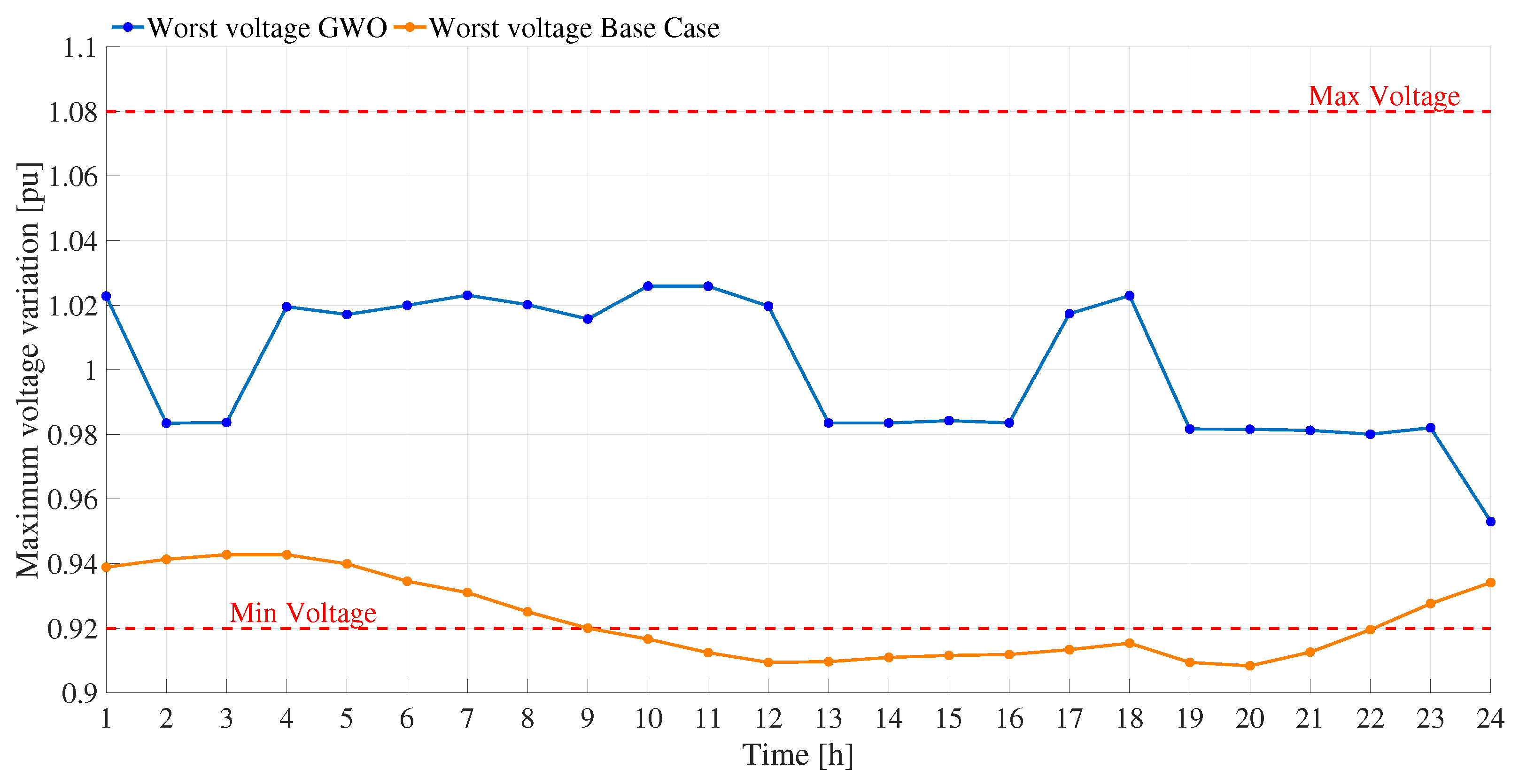
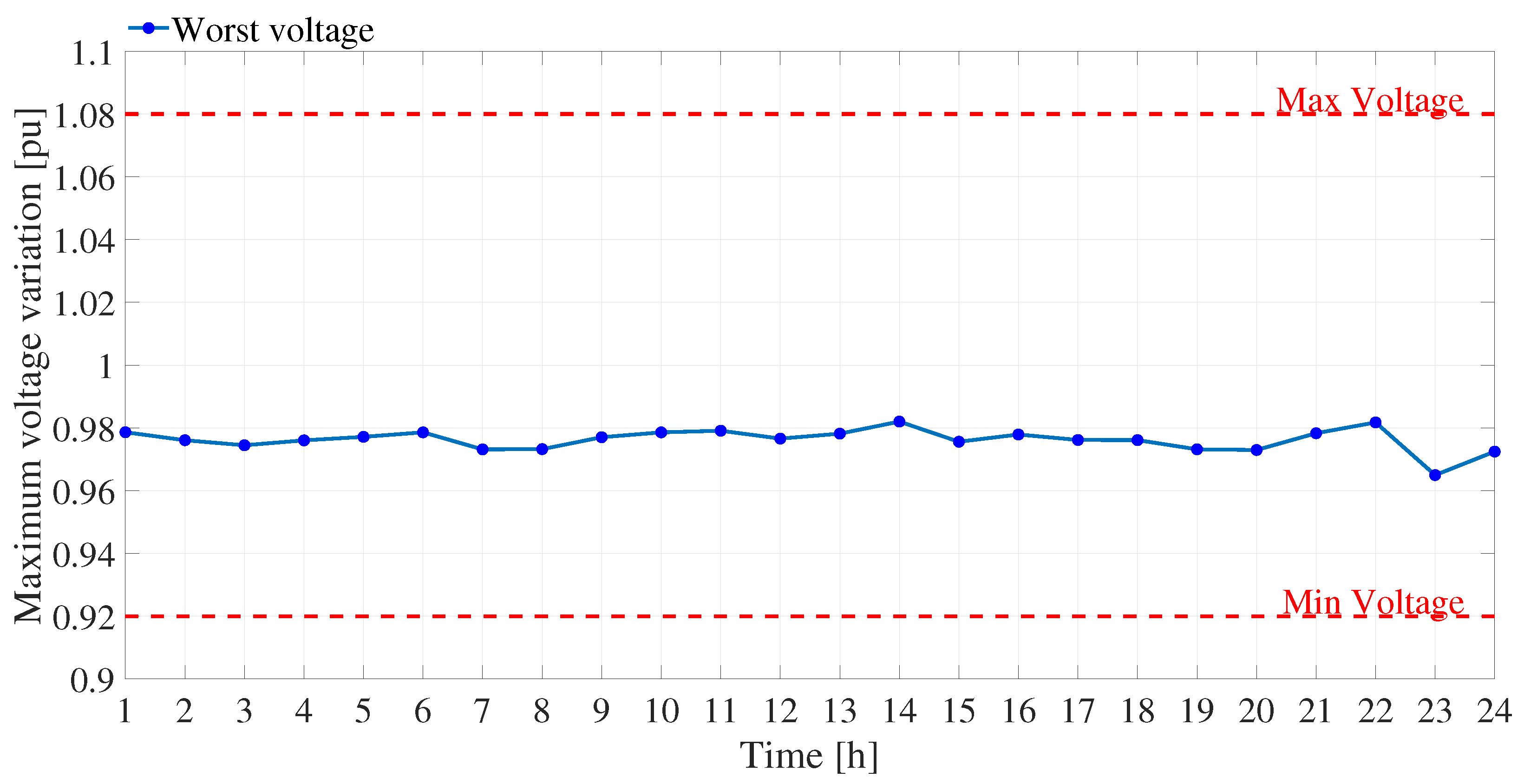
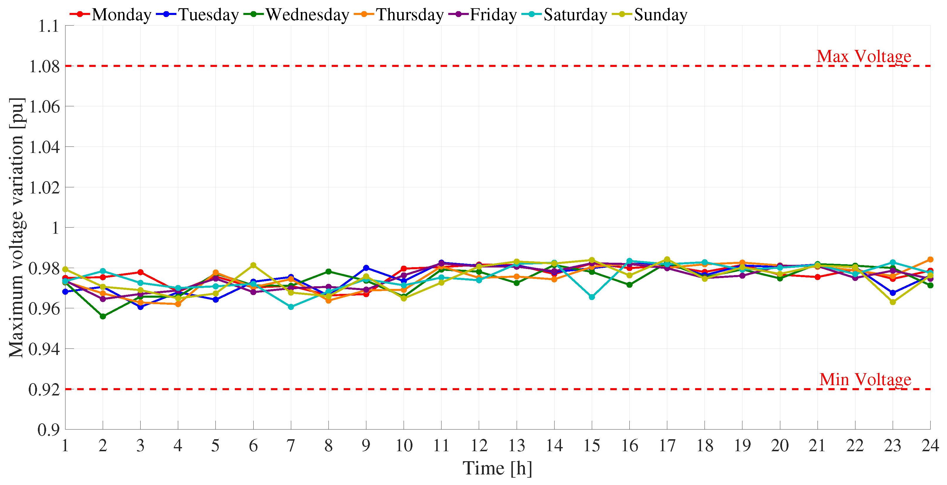
Figure 12 presents the worst nodal voltage at each analyzed time period h, representing the maximum voltage variation in the system. The figure compares the voltage profiles obtained for the base case, without DER generation, and for the best solution provided by the proposed GWO-based optimization strategy. In the base case, the voltage levels violate the operational limits imposed for the microgrid, highlighting the inadequacy of the system without the support of distributed energy resources. In contrast, the solution obtained through the proposed GWO methodology maintains all voltage levels within the specified limits across the entire network and achieves an average voltage improvement of 8.47%. The analysis confirms that the GWO method consistently ensures compliance with the assigned voltage limits throughout the entire operating horizon. These results demonstrate that the proposed GWO-based strategy not only achieves the lowest operational costs compared to the other evaluated methodologies but also significantly enhances voltage stability in the microgrid.

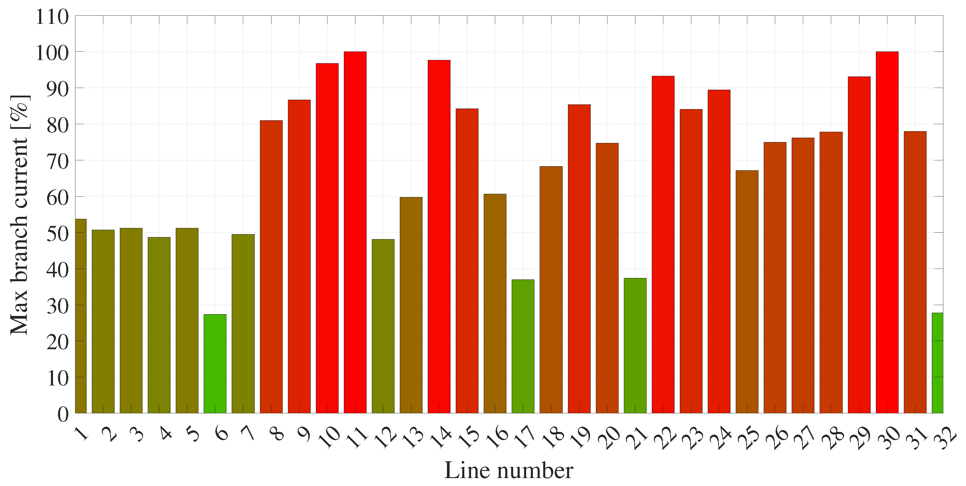
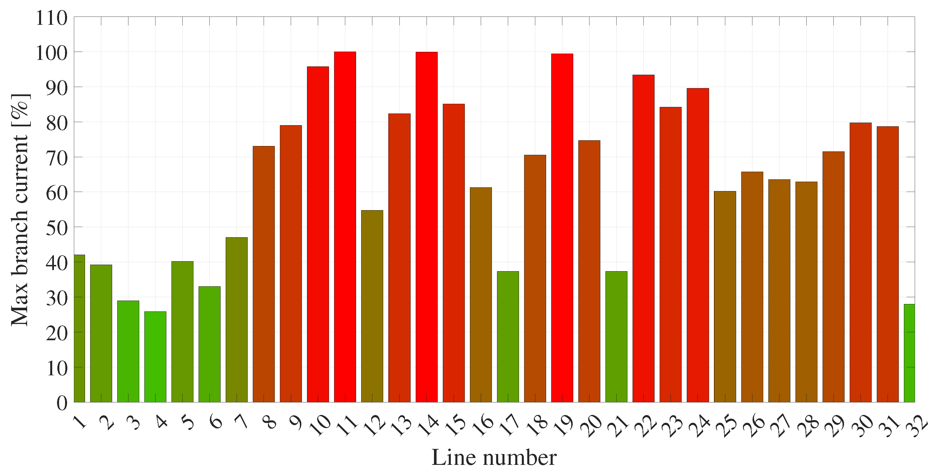
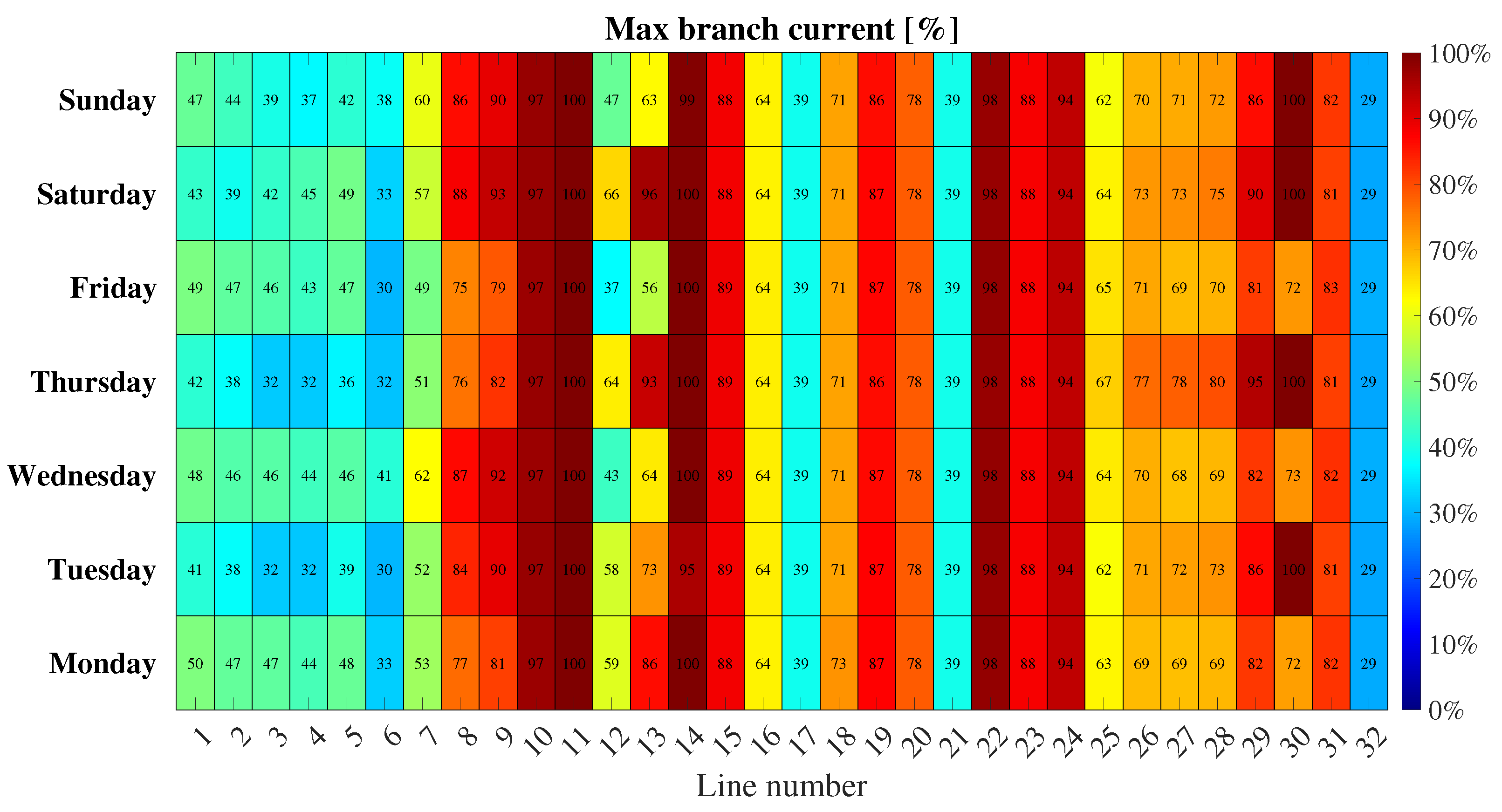
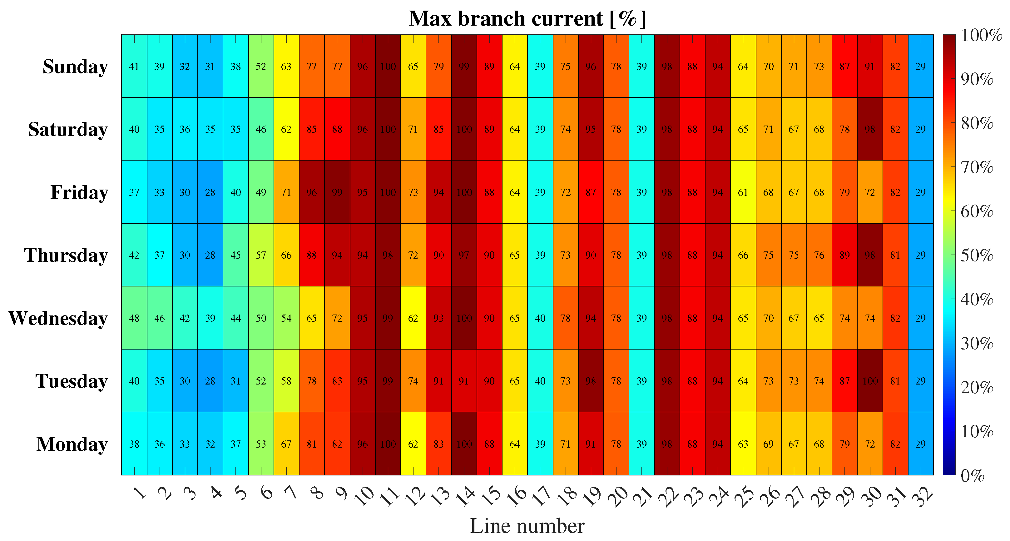
For the maximum line current level across all branches of the AC microgrid, Figure 13 demonstrates that all branches comply with the predefined maximum current limits. The values remain between 0% and below 100%, ensuring that the proposed methodology effectively maintains current within permissible limits.

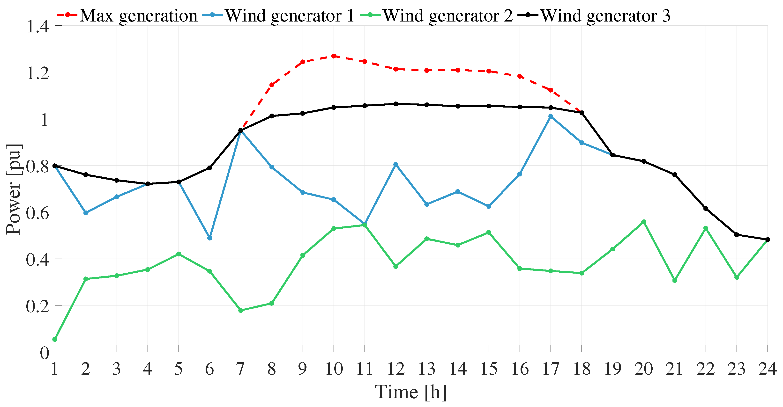
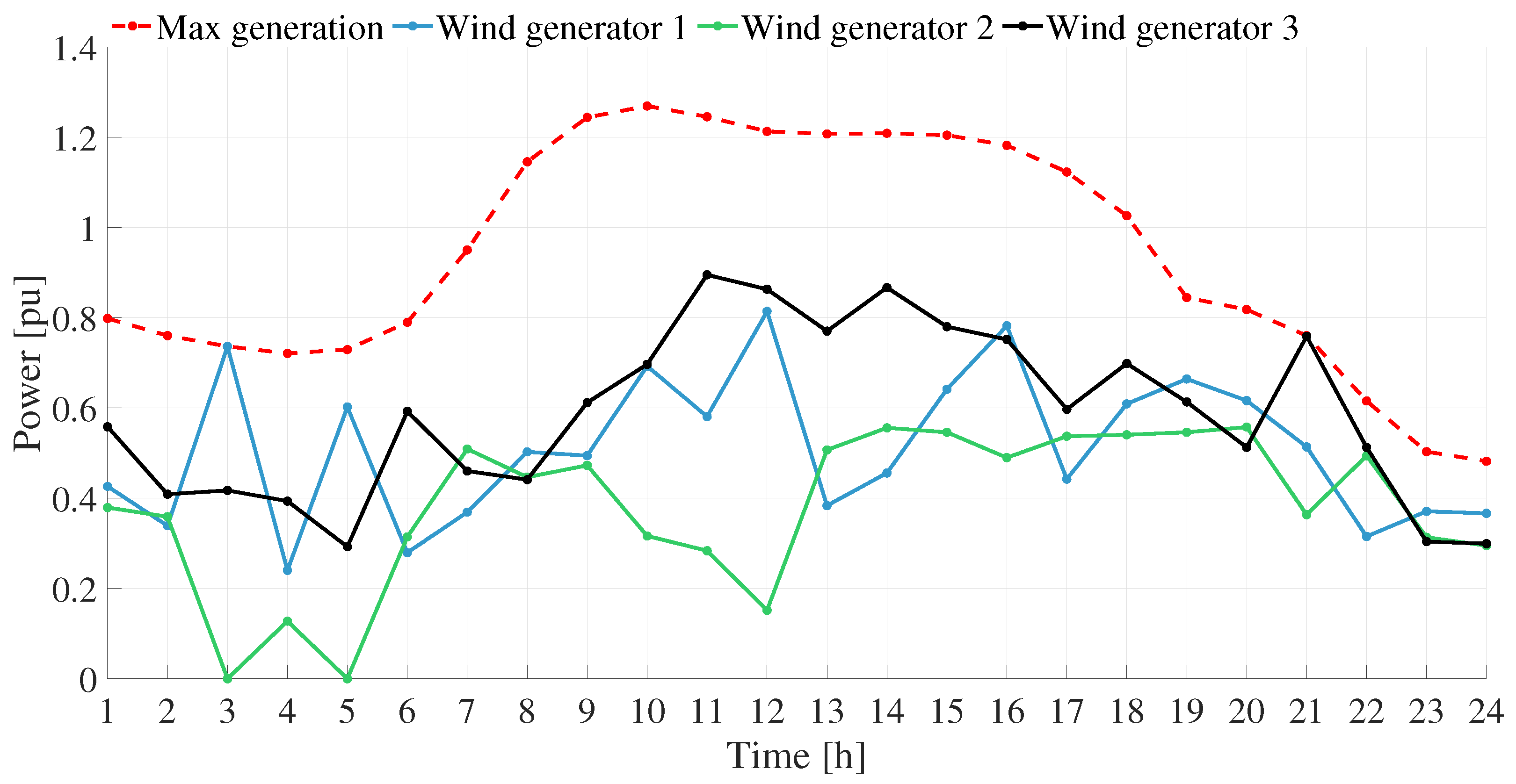
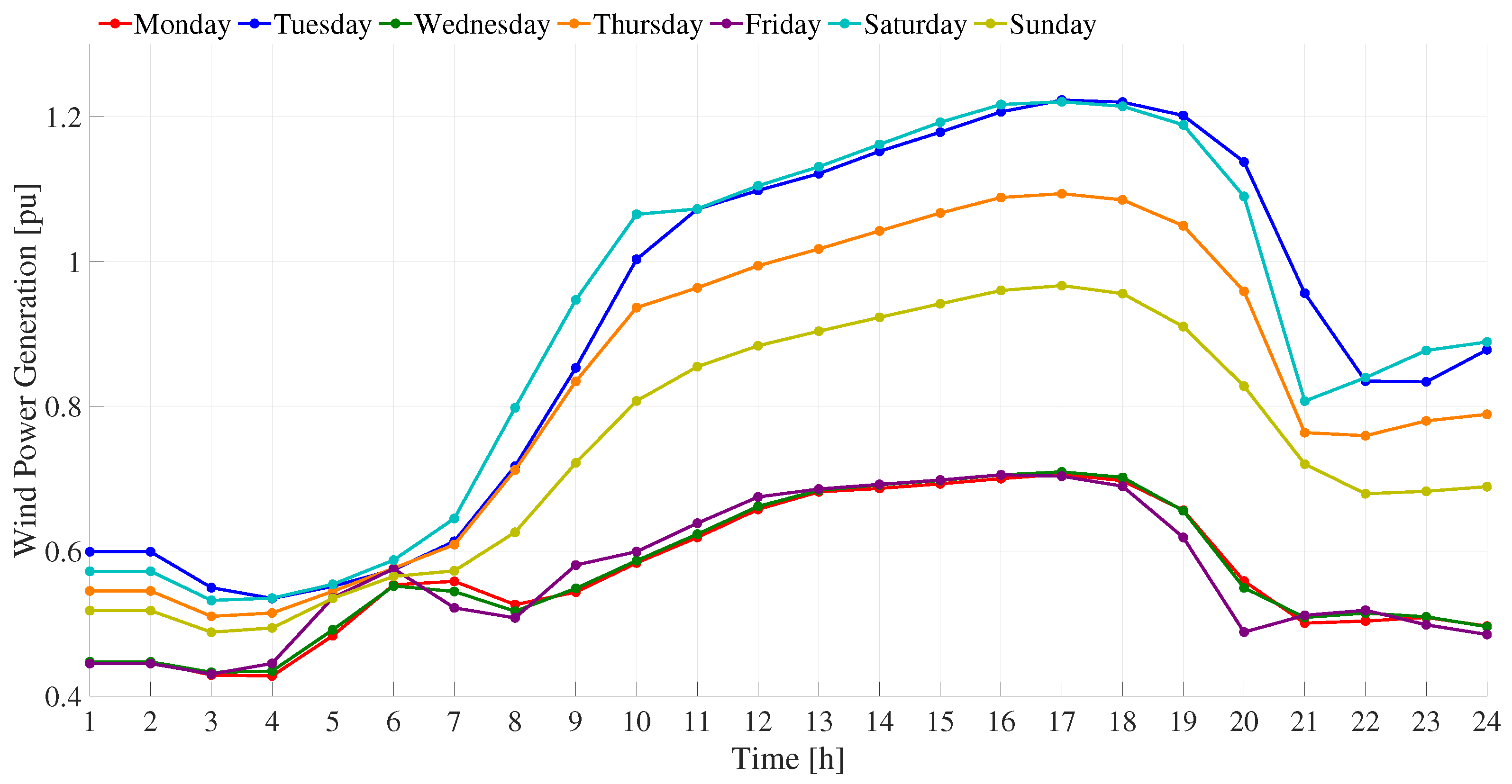
Figure 14 shows the power injected by the WGs during the operating day in on-grid mode. It can be observed that none of the WGs exceed their maximum generation value. The output of each generator varies according to its local wind profile, reflecting the distributed nature of the resource and its influence on system operation.

Between hours 1 and 6, the three WGs exhibit low and fluctuating output, remaining below 0.8 p.u. This period corresponds to low system demand and reduced energy costs, facilitating the charging of BESSs 1 and 3 without significant reliance on wind generation. During this time, WG 3 operates under maximum power point conditions, as its location within the network allows it to exploit the available wind potential fully.

From hours 7 to 12, wind power increases notably. WG 3 reaches stable values close to its upper generation limit, while WG 1 and WG 2 provide moderate but variable outputs. This period coincides with rising demand and energy costs, and the total wind contribution approaches the system’s maximum wind capacity. The increased availability of renewable energy supports the discharge of BESS units and reduces the need for reactive support from D-STATCOMs. However, not all the available wind power is injected into the grid, as the dynamics between generation and demand within the microgrid prevent full utilization of this upper level, reflecting the limitations imposed by local load profiles and operational constraints.

During hours 13 to 18, WG 3 maintains a high and stable output, playing a leading role in sustaining the supply during peak demand. WG 2 and WG 3 continue operating with moderate variability, complementing the overall generation, while WG 1 increases the power level injection. This behavior is consistent with the full discharge of BESSs 1 and 3 and the active operation of D-STATCOM 1 to maintain voltage stability.

In the evening period (19–24), WG 1 and WG 2 show increased fluctuation, while WG 3 gradually reduces its output as wind conditions decline. The total wind power contribution decreases, aligning with a drop in demand and energy prices. During this interval, BESS 2 charges in preparation for the next day, while other units remain inactive or operate minimally.

The behavior of the wind generators directly influences the operational planning of the energy storage systems and support devices. Their hourly generation patterns determine optimal charging and discharging periods, contribute to maintaining voltage levels, and influence energy cost dynamics. The coordinated response of all distributed resources ensures the technical and economic efficiency of the microgrid.

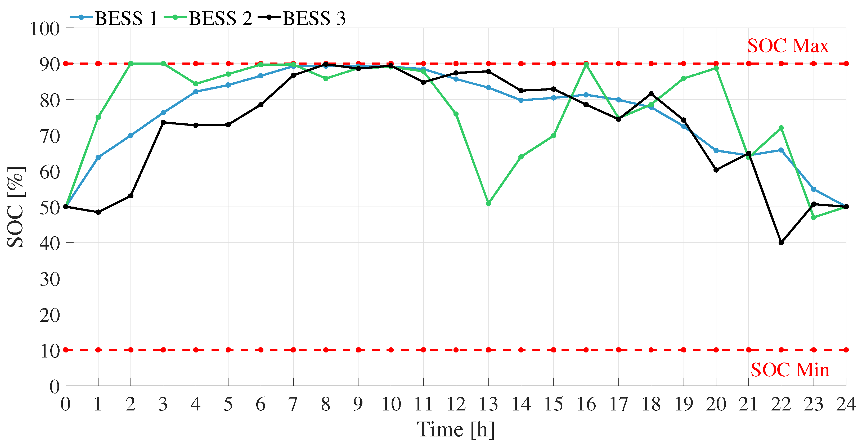
Figure 15 shows the batteries’ state of charge throughout the operating day in on-grid mode. Following IEEE recommendations [36], the initial SoC and final SoC are set to 50%. During the operating period, none of the established SoC limits are exceeded. This figure shows the state of charge evolution for the three battery energy storage systems (BESS 1, BESS 2, and BESS 3) over 24 h. This behavior is directly correlated with the trends in demand, renewable generation, and variable energy cost, as shown in Figure 7. The operational strategy follows a coordinated dispatch aligned with the system’s economic and technical conditions.

During the early hours (1–6 h), BESS 1 and BESS 3 rapidly increased their SoC, taking advantage of a low-demand, low-cost, and low-generation scenario. These systems were charged strategically during off-peak hours when energy is cheaper and easier to store. In contrast, BESS 2 maintained a low and stable SoC, remaining inactive in this interval to not increase the total operational cost of the microgrid.

Between hours 7 and 11, when demand and generation peaked, BESS 1 and BESS 3 reached maximum SoC levels and initiated discharge operations. This was executed to inject energy into the system at times of higher cost and higher demand, contributing to load support and cost reduction. BESS 2, however, remained at a low SoC, still not entering into operation.

From hours 12 to 17, the strategy focused on maximizing energy contribution during a period of sustained high demand and elevated energy costs. BESS 1 and BESS 3 actively discharged energy, reaching SoC levels close to the minimum thresholds defined in the model. In contrast, BESS 2 remained in standby mode, conserving its stored energy for a later time window.

At the beginning of the evening (18–21 h), BESS 1 and BESS 3 reached their minimum SoC levels, while BESS 2 began to charge aggressively due to the simultaneous decrease in both generation and energy cost. This recharging occurred during a period of lower demand, reflecting a strategic operational shift to prepare BESS 2 either for the final hours of the current cycle or for early operation the next day.

Finally, during hours 22 to 24, BESS 2 discharged part of its stored energy to support the system under low-generation nighttime conditions. However, as established by the energy management strategy, it did not discharge below the 50% SoC threshold, to comply with the initial energy condition required for the following day. Meanwhile, BESS 1 and BESS 3 remained idle until hour 23, when they began charging in response to the low energy cost. Both systems charged up to the 50% SoC limit defined in the model, ensuring sufficient reserves to initiate operations effectively the next day.

This staggered and coordinated operation among the three BESS units ensures system balance, cost optimization, and effective use of renewable generation. Each storage system operates in different time windows based on its roles and the dynamic conditions of the system.

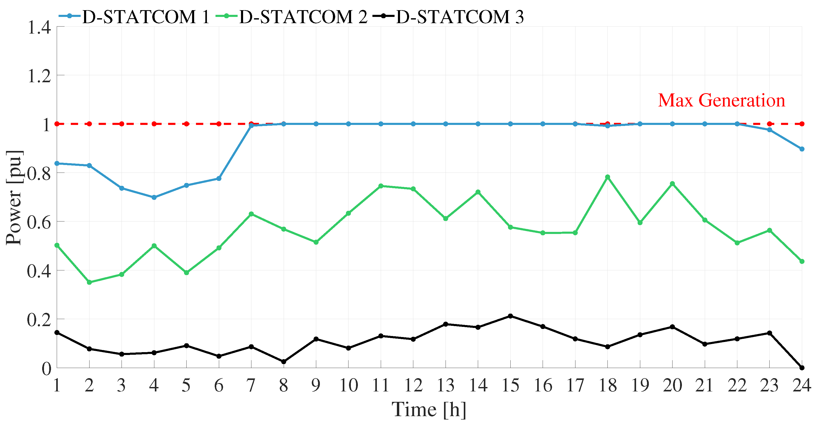
Figure 16 shows the power injected by the D-STATCOMs during the operating day in on-grid mode. All units operate within their predefined power limits (not exceeding 1.0 p.u.), ensuring that voltage regulation and line loading constraints are respected throughout the 24 h cycle.

Between hours 1 and 6, D-STATCOM 1 and D-STATCOM 2 operate at power levels ranging from 35% to 83% of their nominal capacity, while D-STATCOM 3 maintains minimal output. This behavior corresponds to a low and stable demand period, during which voltage regulation requirements are reduced and localized compensation is sufficient to maintain system stability. Notably, D-STATCOM 1, located at the most critical node (node 5) regarding voltage regulation, exhibits the highest compensation levels among the three units, confirming that its placement responds to a higher local need for reactive power support.

From 7 to 12 h, D-STATCOM 1 reaches its maximum output (1.0 p.u.), contributing significantly to voltage control, especially during increasing load and rising energy costs. D-STATCOM 2 also increases its output following load and generation patterns, while D-STATCOM 3 maintains a low but consistent operation.

During 13 to 18 h, demand and cost remain high, and D-STATCOM 1 continues operating near maximum levels. D-STATCOM 2 exhibits a fluctuating pattern, adapting to localized voltage needs, while D-STATCOM 3 contributes modestly. The coordination with the BESS discharge during these hours is evident, as both systems contribute to grid support.

Between 19 and 24 h, the outputs of all D-STATCOMs decrease progressively, aligned with the drop in demand and energy cost. D-STATCOM 2 shows an operational peak near hour 20, likely responding to localized loading effects, while D-STATCOMs 1 and 3 gradually reduce their injection.

The D-STATCOMs operated within their nominal limits throughout the cycle, demonstrating technically adequate performance. However, the observed dynamics revealed that, although they performed as efficiently as possible, their size and location within the network directly influenced their operational scheme. Their activation patterns were driven by load distribution, each device’s specific location and capacity, and the need to maintain voltage levels and line loading within permissible limits. This behavior is directly influenced by the operation of distributed generation, the coordinated charging and discharging of battery storage systems, and the hourly evolution of demand. The interaction among these DERs demonstrates that their combined operation must be analyzed as a correlated system, where the performance of each component affects and complements the others to ensure overall grid stability and optimal operation.

5.4.2. Off-Grid Case

In this subsection, the behavior of all power devices is analyzed, along with the voltage and current constraints associated with microgrid operation.

Figure 17 displays the maximum voltage variation across the system’s nodes over 24 h, operating in off-grid mode. Notably, at no point do the recorded voltages exceed the predefined limits.

Regarding Figure 18, the maximum ampacity of the lines during the operating day in off-grid mode is depicted. It is important to note that, under no circumstances, do the lines exceed their maximum capacity limit.

Figure 19 displays the power supplied by the WGs during the operating day in off-grid mode. It is highlighted that none of the WGs surpass their maximum generation capacity.

In islanded mode, the wind generators exhibit a more irregular operating profile and lower utilization of their maximum generation potential, as observed in Figure 19. During hours 1 to 6, all three generators operate at low power levels with high variability. WG 2, in particular, shows near-zero output at several points. This behavior reflects not only fluctuating wind conditions at each generator’s location but also the operational constraints of the islanded mode, which lacks the flexibility of a main grid to absorb surplus energy.

Between hours 7 and 12, although the available wind potential reaches its peak (as indicated by the “Max generation” curve), the actual output of the generators remains well below this maximum. WG 3 achieves relatively stable generation, while WG 1 and WG 2 continue to operate intermittently. The mismatch between generation and demand prevents full utilization of wind resources, as the microgrid must maintain instantaneous power balance without external support.

From hours 13 to 18, generation levels stabilize slightly. WG 3 maintains high output, while WG 1 and WG 2 show moderate contributions with continued fluctuations. This period coincides with peak demand, and the generators operate in coordination to meet system needs, though their output is still limited by technical and locational constraints.

In the final hours of the day (19 to 24), overall wind generation decreases. The decline in wind availability and lower demand levels lead to reduced output from all generators. WG 2 again drops to minimal values, while WG 1 and WG 3 operate near their lower generation levels.

This behavior highlights the operational limitations of wind generation in isolated microgrids. The absence of grid support restricts the ability to absorb surplus energy, resulting in the underutilization of renewable resources. Compared to the grid-connected mode, where wind generators maintain more stable and higher outputs, the islanded scenario reveals the importance of strategic energy storage deployment to buffer variability and enable efficient use of distributed generation.

Regarding Figure 20, the state SoC of the system’s batteries during the operating day in off-grid mode is illustrated. An initial and final SoC of $50\%$ is assumed. Throughout the operating period, it is evident that none of the defined SoC limits are exceeded.

Figure 20 presents the state of charge profiles of the three battery energy storage systems (BESSs) operating in islanded mode. All units begin the day at 50% SoC, as defined by the system’s energy management policy, and it is evident that none of the defined SoC limits are exceeded. Throughout the first hours (1–6 h), BESS 1 and BESS 3 increase their charge rapidly, reaching values close to the maximum threshold (90%), while BESS 3 follows a more gradual charging pattern.

Between hours 7 and 12, all BESS units maintain high and stable SoC levels, with no significant discharge events. This reflects a conservative operational strategy aimed at preserving energy reserves, considering the system operates without external backup.

During hours 13 to 20, a progressive discharge is observed in BESS 1 and BESS 3, while BESS 2 undergoes a deeper discharge followed by a charging phase, contributing to the dynamic balance of the microgrid and taking advantage of the available renewable energy. Despite these variations, none of the units reach the minimum SoC limit. The strategy prioritizes maintaining sufficient stored energy to face potential fluctuations in demand and renewable generation. Finally, during the last hours of the day (21–24 h), a slight reduction in SoC is observed, and all BESS units reach the target level of 50%, ensuring readiness for the following day’s operating conditions.

In comparison, Figure 15 shows the SoC behavior of the same BESS units under grid-connected conditions. In this case, the batteries exhibit a more dynamic profile. BESS 1 and BESS 3 charge during low-demand, low-cost periods and discharge fully during peak hours, even reaching the minimum SoC limit. BESS 2 operates later in the day, charging strategically in the evening and ending the cycle at 50%.

The key difference between both modes lies in the presence of a variable energy cost signal in the grid-connected scenario. This economic reference allows for a more flexible and optimized use of storage resources, enabling deeper discharges and better alignment with system needs. In contrast, islanded mode requires greater operational caution. The absence of price signals forces the system to rely solely on technical variables, such as demand, generation, and SoC, for decision-making, which reduces responsiveness and increases operational complexity.

Figure 21 shows the hourly power injection of the three D-STATCOMs under islanded operation. In this mode, the three units operate below their nominal capacity at all times, with fluctuating outputs that respond to local voltage regulation needs. D-STATCOM 1 and D-STATCOM 2 exhibit higher variability, with power levels generally between 0.25 and 0.83 p.u., while D-STATCOM 3 operates with lower and more stable outputs, consistently below 0.4 p.u.

This behavior reflects the localized and demand-dependent nature of voltage support in the absence of grid coupling. Without external regulation, each D-STATCOM adapts dynamically to maintain voltage stability and manage line loading based on the operating conditions of its respective node.

In comparison, under grid-connected conditions (Figure 16), D-STATCOM activation is more structured and aligned with system-wide power flows and reactive compensation strategies. In that case, the control scheme allows better coordination between D-STATCOMs and other distributed energy resources, optimizing their use during high-load or high-cost periods.

The islanded scenario reveals the increased complexity of maintaining voltage profiles without centralized coordination. It also highlights the importance of strategic placement and sizing of D-STATCOM units, as their effectiveness is more dependent on local conditions in the absence of grid support.

5.5. Operational Analysis Under Weekly Disturbance Scenarios

To incorporate the effects of power generation and demand variations on the solution’s performance, this section considers an average week of operation in a Colombian microgrid. Figure 22 shows the wind power generation profiles for all days of the week, while Figure 23 presents the corresponding power demand profiles.

The wind generation behavior was modeled using Artificial Neural Networks, based on weather conditions typical of tropical countries such as Colombia [27]. Meanwhile, the weekly power demand data were obtained from an electrical distribution company in Colombia and included four distinct load profiles corresponding to different days of the week: Monday, Tuesday, Thursday, and Friday (regular days); Wednesday; Saturday; and Sunday.

For the simulations performed for each day and under both grid-connected and standalone operation modes, the same microgrid configuration, distributed energy resources, and operational and maintenance cost data used in the original case study were maintained.

The analysis of the results presented in

Table 7. Summary of daily operational costs under grid-connected and isolated modes.

Mode	Monday	Tuesday	Wednesday	Thursday	Friday	Saturday	Sunday	Average
Grid-Connected Mode
Base Case [USD]	8439.98	8439.98	8266.20	8439.98	8439.98	8225.40	7966.71	–
GWO [USD]	3167.37	2468.31	3021.59	2527.93	3155.48	2318.85	2281.95	–
Reduction [USD]	5272.61	5971.68	5244.62	5912.05	5284.50	5906.55	5684.76	5610.97
Reduction [%]	62.47%	70.76%	63.45%	70.05%	62.61%	71.81%	71.36%	67.50%
Isolated Mode
Base Case [USD]	–	–	–	–	–	–	–	–
GWO [USD]	11,377.04	11,353.77	11,358.85	11,355.43	11,366.65	11,362.02	11,341.40	11,359.30

highlights the performance differences between the on-grid and isolated operation modes.

In on-grid mode, the application of the proposed GWO-based strategy resulted in substantial daily operational cost reductions compared to the base case. On average, a cost reduction of 67.50% was obtained across the evaluated week, with daily reductions varying between 62.47% and 71.81%. This low variation range, with a standard deviation of approximately 3.65%, demonstrates the high consistency and reliability of the proposed optimization strategy throughout different operating conditions typically encountered during a week. These results confirm the effectiveness of the proposed methodology in minimizing operational costs by intelligently managing active and reactive power from DERs integrated into the microgrid.

In isolated mode, a base case reference is not available because the microgrid cannot operate without the coordinated action of all installed DERs, including wind turbines, D-STATCOM devices, and BESS. In this mode, the GWO algorithm was responsible for optimizing the operation of the distributed resources to ensure energy supply, voltage support, and system stability. The daily operational costs in isolated mode remained highly stable throughout the week, with an average value of 11,359.30 USD and a very low variation of just 0.12% between days. This minimal fluctuation reflects the robustness and high quality of the solutions obtained, even under the more demanding conditions of standalone microgrid operation.

Finally, to demonstrate that the solutions obtained satisfy the voltage bounds established for the microgrid, Figure 24 and Figure 25 show that the worst voltage value obtained at each operating hour remains within the maximum and minimum voltage limits of ±8% set for the microgrid for each day of operation.

Regarding the maximum current flowing through the lines during the 24 h of operation, Figure 26 and Figure 27 illustrate the maximum current percentage observed across all lines of the microgrid for each hour of operation. From these figures, it can be appreciated that all line currents remain at or below the 100% limit established for safe operation. These results demonstrate that the GWO-based strategy effectively ensures compliance with operational constraints related to line capacities throughout the entire analysis week, guaranteeing the secure and reliable operation of the microgrid under both modes.

6. Conclusions

6.1. Summary of Contributions and Results

This paper presented an optimized energy management strategy for AC microgrids integrating wind generation, BESSs, and D-STATCOMs. The objective was to minimize operational costs in both on-grid and islanded modes while maintaining compliance with system constraints such as voltage levels, current limits, and power balance. The methodology combines a master–slave structure where the GWO performs resource scheduling, and SA evaluates system feasibility.

An in-depth performance analysis of the classical GWO with linear convergence control (GWO-O) was conducted under both on-grid and isolated microgrid operation modes. The results demonstrated that GWO-O consistently underperformed, exhibiting severe degradation in solution quality, consistency, and computational efficiency compared to state-of-the-art methods. In contrast, the proposed modification for controlling the convergence factor significantly enhanced the performance of GWO, achieving notable improvements in minimizing operational costs, energy losses, and $C{O}_2$ emissions. These findings highlight the effectiveness of the proposed approach in addressing complex energy management problems in modern microgrids.

The methodology was tested on a 33-node microgrid using real wind and demand profiles from a Colombian region. Compared with PSO and GA, GWO consistently produced the best results: $3299.39 in on-grid and $11,367.76 in off-grid mode, with the lowest variability (0.19% standard deviation).

Additionally, the average voltage deviation across all nodes was reduced by 2.9% in on-grid mode and 3.5% in off-grid mode, confirming improved voltage regulation and enhanced grid stability.

The technical analysis confirmed that the proposed GWO-based approach ensures strict compliance with operational constraints, including voltage, line current, and battery SoC limits. The addition of reactive power compensation through D-STATCOMs contributed to superior voltage stability and minimized the risk of voltage violations by approximately 80% compared to scenarios without coordinated compensation.

To validate the effectiveness of the proposed GWO-based energy management strategy under variable generation and demand scenarios, a one-week operation was considered, incorporating realistic variations in wind power generation and load demand profiles representative of typical conditions in tropical regions. The results demonstrated that the GWO-based methodology achieved a significant average operational cost reduction of 67.50% in on-grid mode, with minimal variability across different days, confirming the consistency and robustness of the optimization approach. In the isolated mode, the GWO successfully managed the optimal coordination of wind turbines, D-STATCOM devices, and battery energy storage systems, maintaining stable operational costs with a very low daily variation of only 0.12%.

These findings confirm that the proposed GWO-based strategy significantly enhances the economic performance of the microgrid while ensuring high-quality, reliable, and replicable solutions under both steady and uncertain operating conditions, reinforcing its potential as an efficient framework for advanced energy management in modern microgrids.

6.2. Limitations of This Study

While the proposed methodology demonstrates strong performance and practical relevance, certain limitations should be acknowledged to contextualize the results. The model assumes perfect forecasting for both wind power generation and load demand, which may not fully capture real-world uncertainties. Also, the optimization framework relies on a centralized control architecture, which may limit its scalability or applicability in decentralized or peer-to-peer microgrid configurations.

6.3. Academic Contributions

From an academic perspective, this study contributes a hybrid optimization framework that integrates metaheuristics with deterministic power flow models, demonstrating high performance in managing both active and reactive power resources.

It offers statistically validated comparisons of GWO, PSO, and GA, filling a methodological gap in the literature where such multi-algorithm evaluations are often missing or under-reported. This provides a valuable benchmark for future studies in microgrid energy management.

6.4. Industrial Implications

The methodology proves to be practical and adaptable to real-world scenarios, including regulatory constraints and variable generation/demand profiles. Its capability to reduce costs while preserving system stability makes it suitable for implementation in industrial, commercial, or rural microgrids.

By ensuring cost-effectiveness and compliance with operational boundaries, this approach supports utility operators in achieving more sustainable and resilient energy distribution.

Looking ahead, it is worth noting that the modular design of the proposed GWO-based optimization framework, combined with the flexibility of the SA power flow solver, makes it inherently scalable to larger microgrid systems with more nodes and DER units. Furthermore, the methodology is adaptable to different microgrid topologies, including both radial and meshed networks, with minor adjustments to the constraint sets and DER parameterization.

6.5. Future Work

Although the proposed methodology demonstrated strong performance, several concrete areas for improvement remain:

• Adaptive penalty strategy: Include penalty factor based on adaptive values for improving the exploration and reducing the processing times to improve the quality of the results obtained for the optimization methodologies.
• Multi-objective optimization: Future extensions could incorporate environmental objectives (like emission reduction) alongside economic performance to address broader sustainability goals.
• Real-time control strategies: Implementing the method in real-time environments using rolling horizon or model predictive control could address short-term generation and demand fluctuations.
• Hardware-in-the-loop (HIL) testing: Integrating the proposed strategy into HIL platforms can validate its practical applicability and responsiveness under real-world operating conditions.
• Uncertainty modeling: The inclusion of stochastic or robust optimization techniques will allow for more accurate handling of uncertainties in renewable generation and load profiles.
• Microgrid coordination: Exploring coordinated energy management across multiple microgrids with peer-to-peer trading and resource-sharing mechanisms could expand the applicability of the method to interconnected systems.

To improve constraint handling and solution diversity, future iterations of this work could incorporate adaptive penalty coefficients, where the weights $F{p}_1$, $F{p}_2$, and $F{p}_3$ dynamically change based on the extent of constraint violations across generations. This would provide finer discrimination between feasible and near-feasible solutions, especially when there are conflicting constraints.

These directions will contribute to more resilient, flexible, and sustainable microgrid operation strategies, ultimately accelerating the adoption of decentralized energy systems.