
A Mixed-Integer Convex Optimization Framework for Cost-Effective Conductor Selection in Radial Distribution Networks While Considering Load and Renewable Variations

 ,
,  ,
,  ,
,  and
and
Abstract
1. Introduction
2. Methodology
2.1. The MI-Convex Formulation
2.1.1. Objective Function
2.1.2. Problem Constraints
2.1.3. Model Characterization
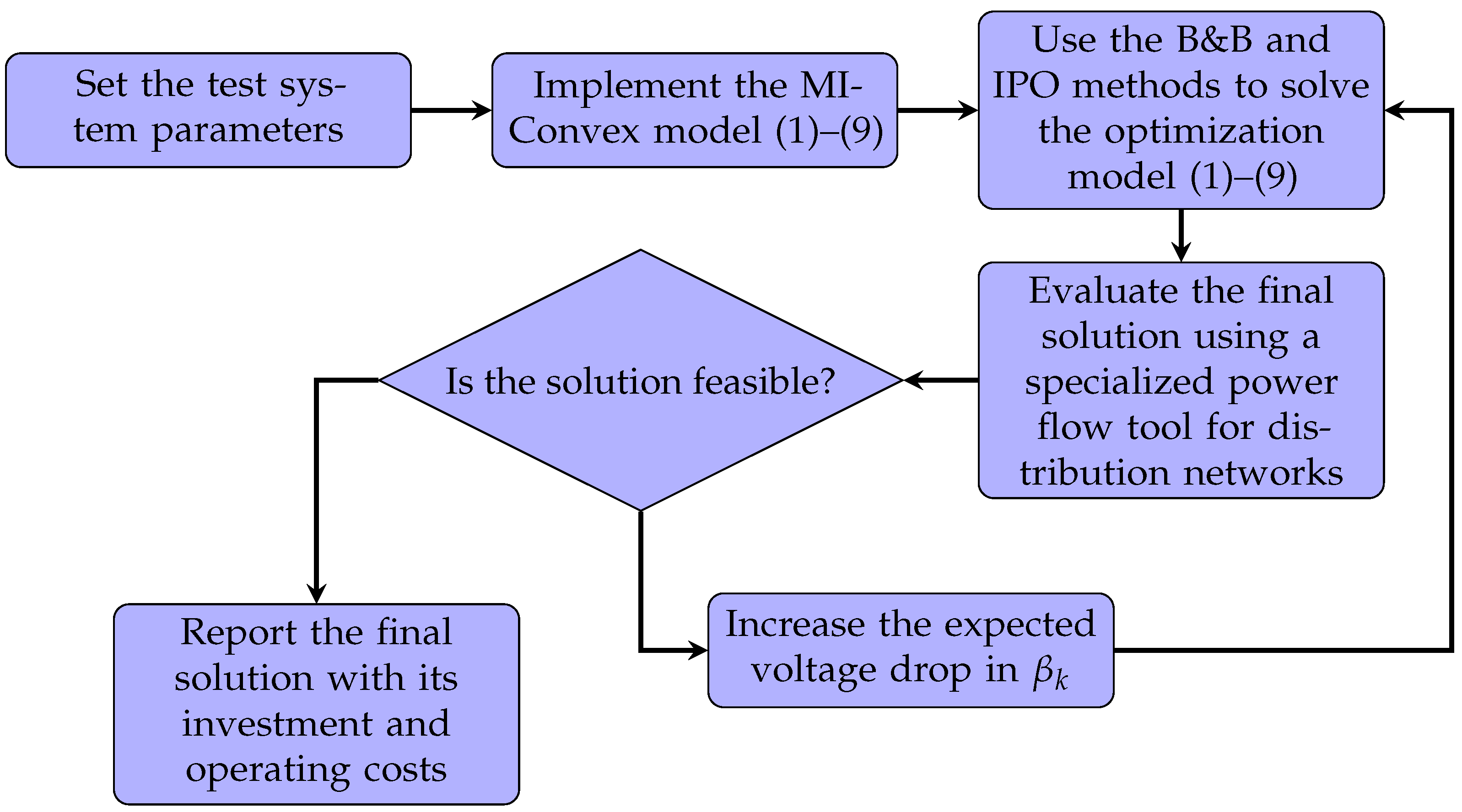
2.2. Solution Strategy
3. Results and Discussion
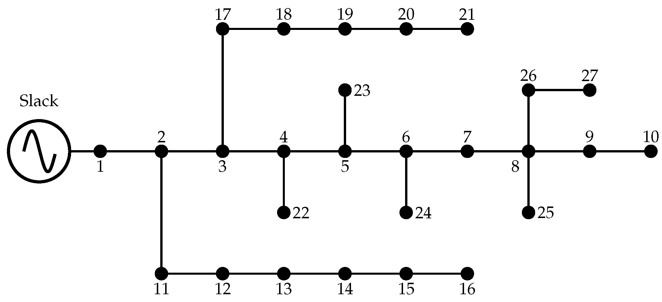
3.1. Test Feeder Characterization
- The 27-bus grid operates using a line-to-ground voltage of at the substation terminals. The total active and reactive power per phase is and , respectively.
- The 33-bus grid operates using a line-to-ground voltage of at the substation terminals. The total active and reactive power per phase is and , respectively.
- The regulatory policies applicable to these feeders define a maximum voltage regulation bound of about .
3.2. Numerical Validations, Analysis, and Discussion
- I
- A comparative assessment against literature-reported results using metaheuristic optimization algorithms under peak load conditions.
- II
- An evaluation of various load curves in order to determine the expected load consumption in the selected conductors.
3.2.1. Peak Load Operating Scenarios
- The total costs of all the plans for the grid vary from US$ 550,680.25 to US$ 561,418.40 for all the optimization methodologies, with the TSA and the proposed MI-Convex approach exhibiting the minimum values and the VSA reporting the maximum value. These results confirm the effectiveness of our proposal in obtaining excellent numerical results, which coincide with the minimum values reported in the specialized literature [17], i.e., they are equal to the solution reported by the TSA.
- The total expected costs of energy losses () exhibit an inverse relationship with the expected investment in conductors (), as observed in the solutions obtained using the VSA and the NMA. This correlation arises because higher investments in conductors lead to the selection of larger gauges, reducing the resistive effects and consequently lowering power losses. Conversely, lower investments result in smaller gauges, increasing the resistive effects and energy losses, as seen in the solutions provided by the GNDO, the TSA, and the MI-Convex method.
- An assessment of the best solution approaches, namely the TSA and MI-Convex within the proposed solution methodology (see Figure 1), reveals that the minimum voltage profile in the 27-bus grid occurs at bus 10, with a voltage value of approximately 0.9745 p.u. This indicates a voltage regulation of about 2.5473% for the test feeder.
- Regarding the expected branch loadability, under peak operating conditions, the distribution line connecting buses 1 and 2 experiences the highest current flow, with a magnitude of approximately 358.164 A. The conductor gauge assigned to this branch is No. 7 (see the first element in the MI-Convex row, the Gauges column), which has a thermal limit of about 600 A. This results in a loadability of approximately 59.6940% for this branch.
- The proposed MI-Convex approach improves upon the numerical results reported by the TSA in [17], achieving an additional reduction of approximately US$ 316.99 in the total objective function. Although this reduction may seem minimal, it confirms the effectiveness of the MI-Convex approach in solving the OCS problem. The key advantage of MI-Convex is its reliability, as it consistently ensures the same numerical solution in every evaluation—which is something that the TSA cannot guarantee.
- The only difference between the TSA and MI-Convex lies in the conductor gauge assigned to the line between nodes 3 and 4 (i.e., line 3). The proposed MI-Convex approach selects gauge No. 7, whereas the TSA uses gauge No. 5. This variation results in a higher conductor investment cost for MI-Convex, totaling US$ 225,372.06, compared to the US$ 209,773.46 required by the TSA. However, as observed in the analysis of the 27-bus grid, higher investment costs lead to reduced power losses, effectively compensating for the increased expenditure and favoring the MI-Convex approach in terms of overall cost-effectiveness.
- The final solution reached with MI-Convex reports its minimum voltage profile at bus 18, with a magnitude of about 0.9629 p.u., which implies that its voltage regulation under peak load conditions is about 3.7093%. This confirms the feasibility of the final solution and an adequate voltage regulation performance.
- Regarding the loadability of all distribution branches for the 33-bus grid under peak load conditions, the maximum value occurs in the branch that connects nodes 4 and 5 (i.e., line 4), with a value of 70.0597%. This confirms the effectiveness of the proposed MI-Convex approach in providing an adequate and effective solution for the OCS problem.
3.2.2. Load Profile Evaluation
- Considering the load behavior has a significant impact on the final distribution system plan, as it directly influences the expected costs of energy losses. In the three-period case, the expected energy losses amount to US$ 183,788.84, representing a reduction of US$ 43,298.33 compared to the peak load scenario. This reduction leads to a decrease of approximately US$ 103,576.50 in conductor investment, as the set of gauges required is adjusted based on the expected energy losses. These variations in both components of the objective function result in a total benefit of US$ 146,874.83 compared to the peak load case.
- The daily operation case shows a slight increase in investment costs, approximately US$ 6,857.25 higher than in the three-period case. This is because the costs of energy losses in the former amount to US$ 212,715.20, which is US$ 28,926.36 more than in the latter. Consequently, larger conductor gauges are selected to mitigate the impact of the squared current flow on the total energy losses calculations. Notably, the daily operating case achieves a cost reduction of approximately 20.17% compared to the peak load scenario, highlighting its effectiveness in optimizing operating expenses.
- The expected costs of energy losses in the three-period and daily operating cases are reduced by approximately 32.41% and 28.63%, respectively, in comparison the peak load scenario. As previously mentioned, this reduction can be attributed to variations in current flow across all distribution branches and to the selection of conductor gauges, which are optimized to effectively balance investment and operating costs.
- The total cost of the distribution system plan is reduced by approximately US$ 117,045.88 and US$ 90,520.84 in the three-period and daily operation scenarios when compared to the peak load case. These reductions confirm that accurate modeling of the expected demand behavior plays a crucial role in determining the investment costs of conductor gauges. When combined with the projected power losses, this directly and significantly impacts the total cost of the distribution system plan.
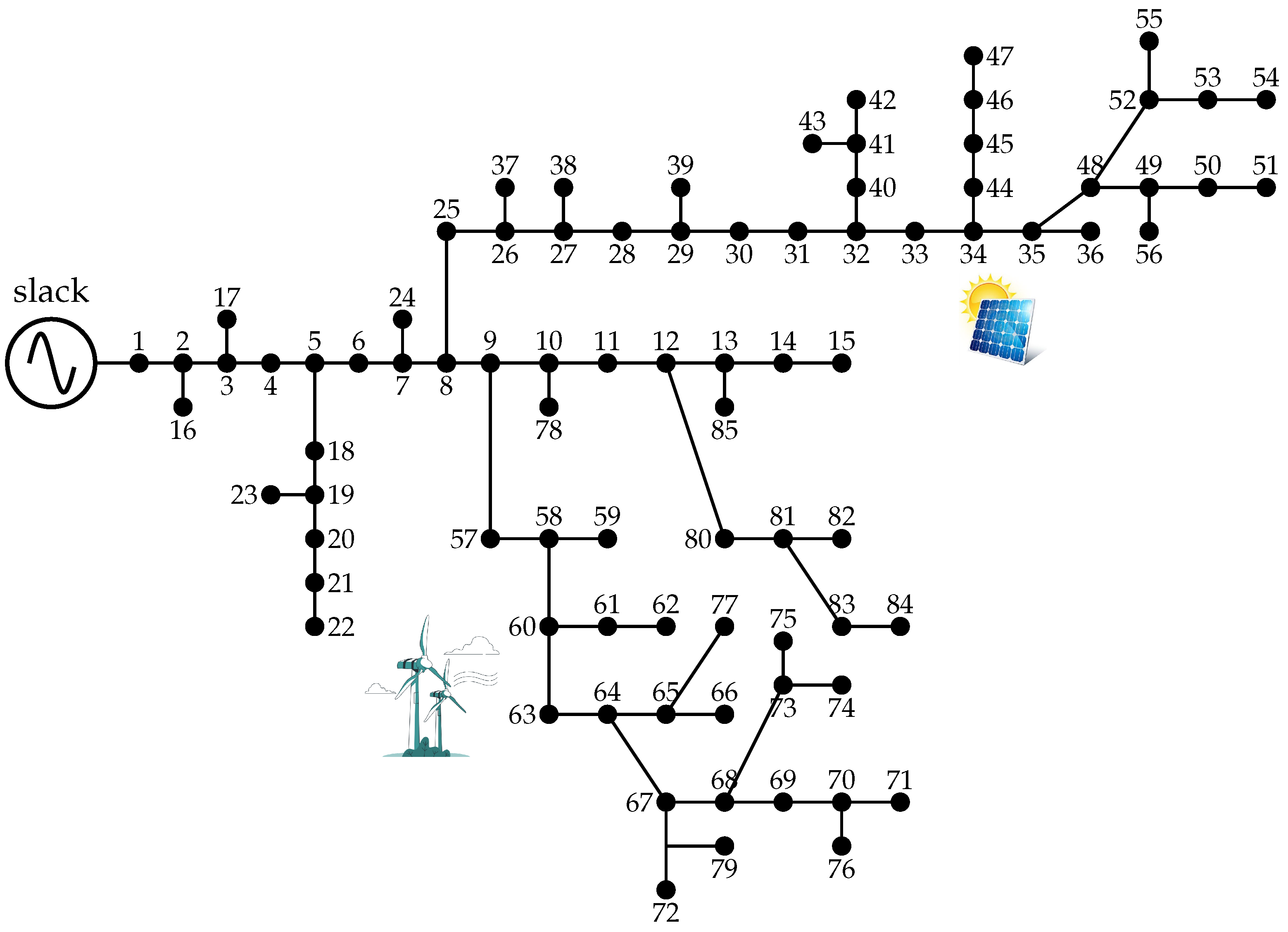
3.3. Large-Scale Distribution Network
- Case 1: An analysis of the optimization framework under peak load conditions, maintaining the same simulation parameters as those used for the 27- and 33-bus grids.
- Case 2: Conductor selection based exclusively on the three-period demand profile.
- Case 3: Conductor selection considering daily load variations, without accounting for the integration of renewable generation sources.
- Case 4: Comprehensive evaluation incorporating both daily demand variations and renewable generation profiles.
- Under peak load conditions, the network is large enough to simultaneously withstand the maximum possible demand across all nodes. This results in the highest total cost (US$ 915,592.73), with US$ 590,252.78 allocated to conductor investment and US$ 325,339.96 to energy losses. The network is heavily oversized because it must account for an extreme – though rare – operational situation, leading to overinvestment in conductor sizes and underutilization during most operating hours.
- When the load profile is segmented into three typical periods (high, medium, and low demand), the total cost is substantially reduced to US$ 739,784.23. Both conductor investment (US$ 434,737.18) and energy losses costs (US$ 305,047.05) decrease compared to the peak load case. This demonstrates that planning based on more realistic demand scenarios prevents unnecessary oversizing, leading to significant cost savings of approximately 19.21%.
- Considering a detailed daily load variation without renewable integration yields a total cost of US$ 787,221.25. Although slightly higher than case 2, this case captures daily consumption fluctuations more precisely, leading to a balanced investment in conductors (US$ 467,893.31) and operational losses reduction (US$ 319,327.95). This approach better reflects the network’s true usage in spite of demand peaks throughout the day.
- The most significant impact is observed when renewable generation is incorporated. The total system cost drops to US$ 705,197.06, even lower than case 3, despite an increase in the costs of energy losses (US$ 314,328.96). This decrease is mainly due to the substantial reduction in conductor investment (US$ 390,868.10)—the lowest among all cases. The presence of DG reduces the net power demand during the day, alleviating current flows across the network and enabling the selection of smaller conductors without compromising system reliability. Thus, renewables minimize infrastructure investment, achieving a cost reduction of about 22.97% compared to the traditional peak-load design.
3.4. Computational Performance Characteristics
- The MI-Convex model shows an expected increase in processing times and the number of total variables as the network size grows (from 27 to 85 buses). Despite the significant rise in variables, especially for the daily operation cases, the solver remains capable of handling large problem instances within reasonable times, particularly for small- and medium-sized grids.
- As the complexity of the scenario increases (from peak load to three-period to daily operation), both the total number of variables and the processing times grow substantially. For example, in the 85-bus grid, the daily operation case requires over 765 s, compared to just 12 s for the peak load scenario, highlighting the computational impact of multi-period modeling.
- The inclusion of DGs in the daily operation case of the 85-bus grid results in a slight reduction in processing times (724.6 s vs. 765.3 s), despite using the same number of variables. This suggests that DG integration can potentially introduce structural changes in the optimization model that favor faster convergence under certain conditions.
4. Conclusions
Author Contributions
Funding
Institutional Review Board Statement
Informed Consent Statement
Data Availability Statement
Acknowledgments
Conflicts of Interest
References
- Byles, D.; Mohagheghi, S. Sustainable power grid expansion: Life cycle assessment, modeling approaches, challenges, and opportunities. Sustainability 2023, 15, 8788. [Google Scholar] [CrossRef]
- Al-Dhaifallah, M.; Refaat, M.M.; Alaas, Z.; Aleem, S.H.A.; El-kholy, E.E.; Ali, Z.M. Multi-objectives transmission expansion planning considering energy storage systems and high penetration of renewables and electric vehicles under uncertain conditions. Energy Rep. 2024, 11, 4143–4164. [Google Scholar] [CrossRef]
- Meinecke, S.; Stock, D.S.; Braun, M. New distributed optimization method for tso–dso coordinated grid operation preserving power system operator sovereignty. Energies 2023, 16, 4753. [Google Scholar] [CrossRef]
- Khattab, H.A.; Aljumah, A.S.; Shaheen, A.M.; Omar, H.A. Improved Manta Ray Foraging Algorithm for Optimal Allocation Strategies to Power Delivery Capabilities in Active Distribution Networks. IEEE Access 2024, 12, 157699–157715. [Google Scholar] [CrossRef]
- Abdelwahab, S.A.M.; El-Rifaie, A.M.; Hegazy, H.Y.; Tolba, M.A.; Mohamed, W.I.; Mohamed, M. Optimal control and optimization of grid-connected PV and wind turbine hybrid systems using electric eel foraging optimization algorithms. Sensors 2024, 24, 2354. [Google Scholar] [CrossRef]
- Gafar, M.; Sarhan, S.; Ginidi, A.R.; Shaheen, A.M. An Improved Bio-Inspired Material Generation Algorithm for Engineering Optimization Problems Including PV Source Penetration in Distribution Systems. Appl. Sci. 2025, 15, 603. [Google Scholar] [CrossRef]
- Obukhov, S.; Ibrahim, A.; Tolba, M.A.; El-Rifaie, A.M. Power balance management of an autonomous hybrid energy system based on the dual-energy storage. Energies 2019, 12, 4690. [Google Scholar] [CrossRef]
- Aljumah, A.S.; Alqahtani, M.H.; Shaheen, A.M.; Ginidi, A.R. Adaptive operational allocation of D-SVCs in distribution feeders using modified artificial rabbits algorithm. Electr. Power Syst. Res. 2025, 245, 111588. [Google Scholar] [CrossRef]
- Alnami, H.; El-Rifaie, A.M.; Moustafa, G.; Hakmi, S.H.; Shaheen, A.M.; Tolba, M.A. Optimal allocation of TCSC devices in transmission power systems by a novel adaptive dwarf mongoose optimization. IEEE Access 2023, 12, 6063–6087. [Google Scholar] [CrossRef]
- Elsayed, A.M.; El-Rifaie, A.M.; Areed, M.F.; Shaheen, A.M.; Atallah, M.O. Allocation and control of multi-devices voltage regulation in distribution systems via rough set theory and grasshopper algorithm: A practical study. Results Eng. 2025, 25, 103860. [Google Scholar] [CrossRef]
- Franco, J.F.; Rider, M.J.; Lavorato, M.; Romero, R. Optimal conductor size selection and reconductoring in radial distribution systems using a mixed-integer LP approach. IEEE Trans. Power Syst. 2012, 28, 10–20. [Google Scholar] [CrossRef]
- Ismael, S.M.; Aleem, S.H.E.A.; Abdelaziz, A.Y. Optimal selection of conductors in Egyptian radial distribution systems using sine-cosine optimization algorithm. In Proceedings of the 2017 Nineteenth International Middle East Power Systems Conference (MEPCON), Cairo, Egypt, 19–21 December 2017; pp. 103–107. [Google Scholar] [CrossRef]
- Zhao, Z.; Mutale, J. Optimal conductor size selection in distribution networks with high penetration of distributed generation using adaptive genetic algorithm. Energies 2019, 12, 2065. [Google Scholar] [CrossRef]
- Cortés-Caicedo, B.; Avellaneda-Gómez, L.S.; Montoya, O.D.; Alvarado-Barrios, L.; Chamorro, H.R. Application of the vortex search algorithm to the phase-balancing problem in distribution systems. Energies 2021, 14, 1282. [Google Scholar] [CrossRef]
- Montoya, O.D.; Molina-Cabrera, A.; Grisales-Noreña, L.F.; Hincapié, R.A.; Granada, M. Improved genetic algorithm for phase-balancing in three-phase distribution networks: A master-slave optimization approach. Computation 2021, 9, 67. [Google Scholar] [CrossRef]
- Guzmán-Henao, J.A.; Cortés-Caicedo, B.; Bolaños, R.I.; Grisales-Noreña, L.F.; Montoya, O.D. Optimal conductor selection and phase balancing in three-phase distribution systems: An integrative approach. Results Eng. 2024, 24, 103416. [Google Scholar] [CrossRef]
- Vélez-Marín, V.M.; Montoya, O.D.; Hernández, J.C. A DIgSILENT Programming-Based Approach for Selecting Conductors in Distribution Networks via the Tabu Search Algorithm. In Proceedings of the 2024 IEEE Colombian Conference on Applications of Computational Intelligence (ColCACI), Pamplona, Colombia, 17–19 July 2024; IEEE: Piscataway, NJ, USA, 2024; pp. 1–6. [Google Scholar]
- Gallego Pareja, L.A.; López-Lezama, J.M.; Gómez Carmona, O. A MILP model for optimal conductor selection and capacitor banks placement in primary distribution systems. Energies 2023, 16, 4340. [Google Scholar] [CrossRef]
- Garces, A. Mathematical Programming for Power Systems Operation: From Theory to Applications in Python; John Wiley & Sons: Hoboken, NJ, USA, 2021. [Google Scholar]
- Ponce, D.; Aguila Téllez, A.; Krishnan, N. Optimal Selection of Conductors in Distribution System Designs Using Multi-Criteria Decision. Energies 2023, 16, 7167. [Google Scholar] [CrossRef]
- Thenepalle, M. A comparative study on optimal conductor selection for radial distribution network using conventional and genetic algorithm approach. Int. J. Comput. Appl. 2011, 17, 6–13. [Google Scholar] [CrossRef]
- Bohórquez-Álvarez, D.P.; Niño-Perdomo, K.D.; Montoya, O.D. Optimal Load Redistribution in Distribution Systems Using a Mixed-Integer Convex Model Based on Electrical Momentum. Information 2023, 14, 229. [Google Scholar] [CrossRef]
- Gadelha, V.; Bullich-Massagué, E.; Sumper, A. Optimal power flow in electrical grids based on power routers. Electr. Power Syst. Res. 2024, 234, 110581. [Google Scholar] [CrossRef]
- de Jesus Delgado, M.A.; Pourakbari-Kasmaei, M.; Rider, M.J. A Branch and Bound algorithm to solve nonconvex MINLP problems via novel division strategy: An electric power system case study. In Proceedings of the 2017 IEEE International Conference on Environment and Electrical Engineering and 2017 IEEE Industrial and Commercial Power Systems Europe (EEEIC/I&CPS Europe), Milan, Italy, 6–9 June 2017; IEEE: Piscataway, NJ, USA, 2017; pp. 1–6. [Google Scholar]
- Androulakis, I.P. MINLP: Branch and bound global optimization algorithm. In Encyclopedia of Optimization; Springer: Berlin/Heidelberg, Germany, 2024; pp. 1–7. [Google Scholar]
- Liu, C.; Ma, Y.; Zhang, D.; Li, J. A feasible path-based branch and bound algorithm for strongly nonconvex MINLP problems. Front. Chem. Eng. 2022, 4, 983162. [Google Scholar] [CrossRef]
- Montoya, O.D.; Gil-González, W. On the numerical analysis based on successive approximations for power flow problems in AC distribution systems. Electr. Power Syst. Res. 2020, 187, 106454. [Google Scholar] [CrossRef]
- Shen, T.; Li, Y.; Xiang, J. A graph-based power flow method for balanced distribution systems. Energies 2018, 11, 511. [Google Scholar] [CrossRef]
- Hoyos Vallejo, J.C.; Quintero Restrepo, J. Comparative Analysis of the Julia and AMPL Computational Tools Used in the Radial Distribution Network Optimization Problem. Ingeniería 2024, 29. [Google Scholar] [CrossRef]
- Dunning, I.; Huchette, J.; Lubin, M. JuMP: A modeling language for mathematical optimization. SIAM Rev. 2017, 59, 295–320. [Google Scholar] [CrossRef]
- Lubin, M.; Dowson, O.; Garcia, J.D.; Huchette, J.; Legat, B.; Vielma, J.P. JuMP 1.0: Recent improvements to a modeling language for mathematical optimization. Math. Program. Comput. 2023, 15, 581–589. [Google Scholar] [CrossRef]
- Pradilla-Rozo, J.D.; Vega-Forero, J.A.; Montoya, O.D. Application of the Gradient-Based Metaheuristic Optimizerto Solve the Optimal Conductor Selection Problemin Three-Phase Asymmetric Distribution Networks. Energies 2023, 16, 888. [Google Scholar] [CrossRef]


| Method | Limitations | Advantages of the MI-Convex Approach |
|---|---|---|
| MILP [11] | Simplifies the nonlinear power flow via linear approximations; may compromise accuracy; not scalable for multi-period or nonlinear load conditions. | Maintains nonlinear power losses modeling through quadratic and conic approximations; supports realistic multi-period demand profiles. |
| SCA [12] | Heuristic; results are not reproducible; requires parameter tuning; no guarantee of global optimality. | Deterministic solution; no parameter tuning; guarantees global optimality due to convex formulation. |
| AGA [13] | Dependent on random initialization; requires calibration of crossover/mutation; high computational cost in large-scale grids. | Solves convex subproblems using interior-point methods; scalable to large networks (e.g., the 85-bus feeder). |
| TSA [17] | Requires large number of iterations; sensitive to stopping criteria; lacks consistent convergence. | Repeatable results; robust convergence using branch-and-bound and interior-point techniques. |
| VSA, GNDO, and NMA | Inconsistent performance across test cases; computational results vary between runs. | Consistent across all runs; reliably minimizes total planning costs; reduced processing times for medium-sized networks. |
| l | k | m | (km) | (kW) | (kvar) |
|---|---|---|---|---|---|
| 1 | 1 | 2 | 0.55 | 0.0 | 0.0 |
| 2 | 2 | 3 | 1.50 | 0.0 | 0.0 |
| 3 | 3 | 4 | 0.45 | 297.5 | 184.4 |
| 4 | 4 | 5 | 0.63 | 0.0 | 0.0 |
| 5 | 5 | 6 | 0.70 | 255.0 | 158.0 |
| 6 | 6 | 7 | 0.55 | 0.0 | 0.0 |
| 7 | 7 | 8 | 1.00 | 212.5 | 131.7 |
| 8 | 8 | 9 | 1.25 | 0.0 | 0.0 |
| 9 | 9 | 10 | 1.00 | 266.1 | 164.9 |
| 10 | 2 | 11 | 1.00 | 85.0 | 52.7 |
| 11 | 11 | 12 | 1.23 | 340.0 | 210.7 |
| 12 | 12 | 13 | 0.75 | 297.5 | 184.4 |
| 13 | 13 | 14 | 0.56 | 191.3 | 118.5 |
| 14 | 14 | 15 | 1.00 | 106.3 | 65.8 |
| 15 | 15 | 16 | 1.00 | 255.0 | 158.0 |
| 16 | 3 | 17 | 1.00 | 255.0 | 158.0 |
| 17 | 17 | 18 | 0.60 | 127.5 | 79.0 |
| 18 | 18 | 19 | 0.90 | 297.5 | 184.4 |
| 19 | 19 | 20 | 0.95 | 340.0 | 210.7 |
| 20 | 20 | 21 | 1.00 | 85.0 | 52.7 |
| 21 | 4 | 22 | 1.00 | 106.3 | 65.8 |
| 22 | 5 | 23 | 1.00 | 55.3 | 34.2 |
| 23 | 6 | 24 | 0.40 | 69.7 | 43.2 |
| 24 | 8 | 25 | 0.60 | 255.0 | 158.0 |
| 25 | 8 | 26 | 0.60 | 63.8 | 39.5 |
| 26 | 26 | 27 | 0.80 | 170.0 | 105.4 |
| l | k | m | (km) | (kW) | (kvar) |
|---|---|---|---|---|---|
| 1 | 1 | 2 | 0.0699 | 100 | 60 |
| 2 | 2 | 3 | 0.3720 | 90 | 40 |
| 3 | 3 | 4 | 0.2762 | 120 | 80 |
| 4 | 4 | 5 | 0.2876 | 60 | 30 |
| 5 | 5 | 6 | 0.7630 | 60 | 20 |
| 6 | 6 | 7 | 0.4030 | 200 | 100 |
| 7 | 7 | 8 | 1.4733 | 200 | 100 |
| 8 | 8 | 9 | 0.8850 | 60 | 20 |
| 9 | 9 | 10 | 0.8900 | 60 | 20 |
| 10 | 10 | 11 | 0.1308 | 45 | 30 |
| 11 | 11 | 12 | 0.2491 | 60 | 35 |
| 12 | 12 | 13 | 1.3115 | 60 | 35 |
| 13 | 13 | 14 | 0.6272 | 120 | 80 |
| 14 | 14 | 15 | 0.5585 | 60 | 10 |
| 15 | 15 | 16 | 0.6457 | 60 | 20 |
| 16 | 16 | 17 | 1.5050 | 60 | 20 |
| 17 | 17 | 18 | 0.6530 | 90 | 40 |
| 18 | 2 | 19 | 0.1603 | 90 | 40 |
| 19 | 19 | 20 | 1.4298 | 90 | 40 |
| 20 | 20 | 21 | 0.4439 | 90 | 40 |
| 21 | 21 | 22 | 0.8231 | 90 | 40 |
| 22 | 3 | 23 | 0.3798 | 90 | 40 |
| 23 | 23 | 24 | 0.8035 | 420 | 200 |
| 24 | 24 | 25 | 0.7985 | 420 | 200 |
| 25 | 6 | 26 | 0.1532 | 60 | 25 |
| 26 | 26 | 27 | 0.2145 | 60 | 25 |
| 27 | 27 | 28 | 0.9963 | 60 | 20 |
| 28 | 28 | 29 | 0.7524 | 120 | 70 |
| 29 | 29 | 30 | 0.3830 | 200 | 600 |
| 30 | 30 | 31 | 0.9687 | 150 | 70 |
| 31 | 31 | 32 | 0.3362 | 210 | 100 |
| 32 | 32 | 33 | 0.4356 | 60 | 40 |
| Gauge c | (/km) | (/km) | (A) | (US$/km) |
|---|---|---|---|---|
| 1 | 0.8763 | 0.4133 | 180 | 1986 |
| 2 | 0.6960 | 0.4133 | 200 | 2790 |
| 3 | 0.5518 | 0.4077 | 230 | 3815 |
| 4 | 0.4387 | 0.3983 | 270 | 5090 |
| 5 | 0.3480 | 0.3899 | 300 | 8067 |
| 6 | 0.2765 | 0.3610 | 340 | 12,673 |
| 7 | 0.0966 | 0.1201 | 600 | 23,419 |
| 8 | 0.0853 | 0.0950 | 720 | 30,070 |
| Method | Gauges | (US$) | (US$) | (US$) |
|---|---|---|---|---|
| VSA | [7,7,5,4,4,3,3,1,1,4,4,2,3,2,1,4,4,2,2,2,1,1,2,2,1,1] | 217,066.25 | 344,352.15 | 561,418.40 |
| NMA | [7,7,4,4,4,4,3,1,1,4,4,3,3,1,2,4,3,2,1,1,1,1,2,2,1,1] | 219,343.86 | 337,744.80 | 557,088.66 |
| GNDO | [7,7,4,4,4,3,3,1,1,4,4,2,1,1,1,3,2,2,1,1,1,1,1,1,1,1] | 230,953.18 | 319,768.08 | 550,721.26 |
| TSA | [7,7,4,4,4,3,3,1,1,4,4,2,1,1,1,4,2,2,1,1,1,1,1,1,1,1] | 227,087.17 | 323,593.08 | 550,680.25 |
| MI-Convex | [7,7,4,4,4,3,3,1,1,4,4,2,1,1,1,4,2,2,1,1,1,1,1,1,1,1] | 227,087.17 | 323,593.08 | 550,680.25 |
| Method | Gauges | (US$) | (US$) | (US$) |
|---|---|---|---|---|
| TSA | [7,7,5,5,5,4,3,2,1,1,1,1,1,1,1,1 | 215,137.5583 | 209,773.4628 | 424,911.0211 |
| 1,1,1,1,1,3,2,1,4,4,4,3,3,1,1,1] | ||||
| MI-Convex | [7,7,7,5,5,4,3,2,1,1,1,1,1,1,1,1 | 199,221.9755 | 225,372.0600 | 424,594.0354 |
| 1,1,1,1,1,3,2,1,4,4,4,3,3,1,1,1] |
| Time (t) | Power (p.u.) | Time (t) | Power (p.u.) |
|---|---|---|---|
| 1 | 0.6845 | 13 | 0.8706 |
| 2 | 0.6441 | 14 | 0.8343 |
| 3 | 0.6131 | 15 | 0.8165 |
| 4 | 0.5997 | 16 | 0.8194 |
| 5 | 0.5889 | 17 | 0.8741 |
| 6 | 0.5980 | 18 | 1.0000 |
| 7 | 0.6268 | 19 | 0.9836 |
| 8 | 0.6517 | 20 | 0.9364 |
| 9 | 0.7060 | 21 | 0.8876 |
| 10 | 0.7870 | 22 | 0.8093 |
| 11 | 0.8390 | 23 | 0.7459 |
| 12 | 0.8527 | 24 | 0.7335 |
| Load Case | Gauges | (US$) | (US$) | (US$) | Min. Voltage (p.u.) |
|---|---|---|---|---|---|
| Peak load scenario | [7,7,4,4,4,3,3,1,1,4,4,2,1, | 227,087.17 | 323,593.08 | 550,680.25 | 0.9745 (Bus 10) |
| 1,1,4,2,2,1,1,1,1,1,1,1,1] | |||||
| Three-period case | [7,5,4,3,3,2,2,1,1,3,2,1,1, | 183,788.84 | 220,016.58 | 403,805.42 | 0.9622 (Bus 10) |
| 1,1,2,1,1,1,1,1,1,1,1,1,1] | |||||
| Daily operation case | [7,5,4,3,3,2,2,1,1,3,3,1,1, | 212,715.20 | 226,873.83 | 439,589.03 | 0.9622 (Bus 10) |
| 1,1,3,1,1,1,1,1,1,1,1,1,1] |
| Load Case | Gauges | (US$) | (US$) | (US$) | Min. Voltage (pu) |
|---|---|---|---|---|---|
| Peak load scenario | [7,7,7,5,5,4,3,2,1,1,1,1,1,1,1,1, | 201,987.52 | 222,494.12 | 424,481.65 | 0.9629 (Bus 18) |
| 1,1,1,1,1,3,2,1,4,4,4,3,3,1,1,1] | |||||
| Three-period case | [7,7,5,4,4,2,1,1,1,1,1,1,1,1,1,1, | 136,498.40 | 170,937.37 | 307,435.77 | 0.9554 (Bus 18) |
| 1,1,1,1,1,1,1,1,3,2,2,2,2,1,1,1] | |||||
| Daily operation case | [7,7,5,5,5,3,2,1,1,1,1,1,1,1,1,1, | 144,208.42 | 189,752.39 | 333,960.81 | 0.9588 (Bus 18) |
| 1,1,1,1,1,2,1,1,3,3,3,2,2,1,1,1] |
| l | k | m | (km) | (kW) | (kvar) | l | k | m | (km) | (kW) | (kvar) |
|---|---|---|---|---|---|---|---|---|---|---|---|
| 1 | 1 | 2 | 0.468 | 0.000 | 0.000 | 43 | 34 | 44 | 0.985 | 35.28 | 35.99 |
| 2 | 2 | 3 | 0.449 | 0.000 | 0.000 | 44 | 44 | 45 | 0.441 | 35.28 | 35.99 |
| 3 | 3 | 4 | 0.323 | 56 | 57.13 | 45 | 45 | 46 | 0.225 | 35.28 | 35.99 |
| 4 | 4 | 5 | 0.870 | 0.000 | 0.000 | 46 | 46 | 47 | 0.184 | 14 | 14.28 |
| 5 | 5 | 6 | 0.883 | 35.28 | 35.99 | 47 | 35 | 48 | 0.698 | 0.000 | 0.000 |
| 6 | 6 | 7 | 0.343 | 0.000 | 0.000 | 48 | 48 | 49 | 0.875 | 0.000 | 0.000 |
| 7 | 7 | 8 | 0.953 | 35.28 | 35.99 | 49 | 49 | 50 | 0.768 | 36.28 | 37.01 |
| 8 | 8 | 9 | 0.309 | 0.000 | 0.000 | 50 | 50 | 51 | 0.261 | 56 | 57.13 |
| 9 | 9 | 10 | 0.931 | 0.000 | 0.000 | 51 | 48 | 52 | 0.985 | 0.000 | 0.000 |
| 10 | 10 | 11 | 0.161 | 56 | 57.13 | 52 | 52 | 53 | 0.448 | 35.28 | 35.99 |
| 11 | 11 | 12 | 0.952 | 0.000 | 0.000 | 53 | 53 | 54 | 0.344 | 56 | 57.13 |
| 12 | 12 | 13 | 0.878 | 0.000 | 0.000 | 54 | 52 | 55 | 0.673 | 56 | 57.13 |
| 13 | 13 | 14 | 0.507 | 35.28 | 35.99 | 55 | 49 | 56 | 0.564 | 14 | 14.28 |
| 14 | 14 | 15 | 0.018 | 35.28 | 35.99 | 56 | 9 | 57 | 0.545 | 56 | 57.13 |
| 15 | 2 | 16 | 0.778 | 35.28 | 35.99 | 7 | 57 | 58 | 0.564 | 0.000 | 0.000 |
| 16 | 3 | 17 | 0.359 | 112 | 114.26 | 58 | 58 | 59 | 0.650 | 56 | 57.13 |
| 17 | 5 | 18 | 0.848 | 56 | 57.13 | 59 | 58 | 60 | 0.237 | 56 | 57.13 |
| 18 | 18 | 19 | 0.433 | 56 | 57.13 | 60 | 60 | 61 | 0.626 | 56 | 57.13 |
| 19 | 19 | 20 | 0.605 | 35.28 | 35.99 | 61 | 61 | 62 | 0.530 | 56 | 57.13 |
| 20 | 20 | 21 | 0.377 | 35.28 | 35.99 | 62 | 60 | 63 | 0.514 | 14 | 14.28 |
| 21 | 21 | 22 | 0.721 | 35.28 | 35.99 | 63 | 63 | 64 | 0.701 | 0.000 | 0.000 |
| 22 | 19 | 23 | 0.316 | 56 | 57.13 | 64 | 64 | 65 | 0.373 | 0.000 | 0.000 |
| 23 | 7 | 4 | 0.949 | 35.28 | 35.99 | 65 | 65 | 66 | 0.614 | 56 | 57.13 |
| 24 | 8 | 5 | 0.849 | 35.28 | 35.99 | 66 | 64 | 67 | 0.307 | 0.000 | 0.000 |
| 25 | 25 | 26 | 0.775 | 56 | 57.13 | 67 | 67 | 68 | 0.322 | 0.000 | 0.000 |
| 26 | 26 | 27 | 0.299 | 0.000 | 0.000 | 68 | 68 | 69 | 0.662 | 56 | 57.13 |
| 27 | 27 | 28 | 0.872 | 56 | 57.13 | 69 | 69 | 70 | 0.150 | 0.000 | 0.000 |
| 28 | 28 | 29 | 0.375 | 0.000 | 0.000 | 70 | 70 | 71 | 0.384 | 35.28 | 35.99 |
| 29 | 29 | 30 | 0.798 | 35.28 | 35.99 | 71 | 67 | 72 | 0.320 | 56 | 57.13 |
| 30 | 30 | 31 | 0.816 | 35.28 | 35.99 | 72 | 68 | 73 | 0.291 | 0.000 | 0.000 |
| 31 | 31 | 32 | 0.999 | 0.000 | 0.000 | 73 | 73 | 74 | 0.213 | 56 | 57.13 |
| 32 | 32 | 33 | 0.045 | 14 | 14.28 | 74 | 73 | 75 | 0.721 | 35.28 | 35.99 |
| 33 | 33 | 34 | 0.236 | 0.000 | 0.000 | 75 | 70 | 76 | 0.705 | 56 | 57.13 |
| 34 | 34 | 35 | 0.430 | 0.000 | 0.000 | 76 | 65 | 77 | 0.715 | 14 | 14.28 |
| 35 | 35 | 36 | 0.847 | 35.28 | 35.99 | 77 | 10 | 78 | 0.361 | 56 | 57.13 |
| 36 | 26 | 37 | 0.386 | 56 | 57.13 | 78 | 67 | 79 | 0.546 | 35.28 | 35.99 |
| 37 | 27 | 38 | 0.122 | 56 | 57.13 | 79 | 12 | 80 | 0.357 | 56 | 57.13 |
| 38 | 29 | 39 | 0.915 | 56 | 57.13 | 80 | 80 | 81 | 0.940 | 0.000 | 0.000 |
| 39 | 32 | 40 | 0.182 | 35.28 | 35.99 | 81 | 81 | 82 | 0.444 | 56 | 57.13 |
| 40 | 40 | 41 | 0.590 | 0.000 | 0.000 | 82 | 81 | 83 | 0.110 | 35.28 | 35.99 |
| 41 | 41 | 42 | 0.812 | 35.28 | 35.99 | 83 | 83 | 84 | 0.865 | 14 | 14.28 |
| 42 | 41 | 43 | 0.261 | 35.28 | 35.99 | 84 | 13 | 85 | 0.300 | 35.28 | 35.99 |
| Time (h) | Demand (pu) | Photovoltaic (pu) | Wind (pu) |
|---|---|---|---|
| 1 | 0.684511335492475 | 0 | 0.633118295 |
| 2 | 0.644122690036197 | 0 | 0.607259323 |
| 3 | 0.613069156029720 | 0 | 0.605557422 |
| 4 | 0.599733282530006 | 0 | 0.684246423 |
| 5 | 0.588874071251667 | 0 | 0.783719339 |
| 6 | 0.598018670222900 | 0 | 0.790557706 |
| 7 | 0.626786054486569 | 0 | 0.744958950 |
| 8 | 0.651743189178891 | 0.0391233650 | 0.769603567 |
| 9 | 0.706039245570585 | 0.0655871790 | 0.826492212 |
| 10 | 0.787007048961707 | 0.2368707960 | 0.876523598 |
| 11 | 0.839016955610593 | 0.4550178180 | 0.931213527 |
| 12 | 0.852733854067441 | 0.7264402650 | 0.965504834 |
| 13 | 0.870642027052772 | 0.9244863260 | 0.972218577 |
| 14 | 0.834254143646409 | 0.9820411530 | 0.981135531 |
| 15 | 0.816536483139646 | 0.8294070790 | 0.991393173 |
| 16 | 0.819394170318156 | 0.7330632950 | 1 |
| 17 | 0.874071251666984 | 0.5011338490 | 0.987258076 |
| 18 | 1 | 0.1771175180 | 0.929542167 |
| 19 | 0.983615926843208 | 0 | 0.791155379 |
| 20 | 0.936368832158506 | 0 | 0.708839248 |
| 21 | 0.887597637645266 | 0 | 0.712881960 |
| 22 | 0.809297008954087 | 0 | 0.719897641 |
| 23 | 0.745856353591160 | 0 | 0.703007456 |
| 24 | 0.733473042484283 | 0 | 0.687238555 |
| Load Case | Gauges | (US$) | (US$) | (US$) | Min. Voltage (pu) |
|---|---|---|---|---|---|
| Case 1 | [7,7,7,7,7,7,7,4,1,1,1,1,1,1,1,1,1,1,1,1,1, | 325,339.96 | 590,252.78 | 915,592.73 | 0.9414 (Bus 54) |
| 1,1,4,4,4,3,3,3,2,2,1,1,1,1,1,1,1,1,1,1,1, | |||||
| 1,1,1,1,1,1,1,1,1,1,1,1,1,3,3,1,2,1,1,1,1, | |||||
| 1,1,1,1,1,1,1,1,1,1,1,1,1,1,1,1,1,1,1,1,1] | |||||
| Case 2 | [7,7,7,6,5,5,5,4,1,1,1,1,1,1,1,1,1,1,1,1,1, | 305,047.05 | 434,737.18 | 739,784.23 | 0.9036 (Bus 54) |
| 1,1,3,3,2,2,1,1,1,1,1,1,1,1,1,1,1,1,1,1,1, | |||||
| 1,1,1,1,1,1,1,1,1,1,1,1,1,2,1,1,1,1,1,1,1, | |||||
| 1,1,1,1,1,1,1,1,1,1,1,1,1,1,1,1,1,1,1,1,1] | |||||
| Case 3 | [7,7,7,7,5,5,5,4,1,1,1,1,1,1,1,1,1,1,1,1,1, | 319,327.95 | 467,893.31 | 787,221.25 | 0.9136 (Bus 54) |
| 1,1,3,3,3,2,2,2,1,1,1,1,1,1,1,1,1,1,1,1,1, | |||||
| 1,1,1,1,1,1,1,1,1,1,1,1,1,2,2,1,1,1,1,1,1, | |||||
| 1,1,1,1,1,1,1,1,1,1,1,1,1,1,1,1,1,1,1,1,1] | |||||
| Case 4 | [7,6,5,5,5,5,5,3,1,1,1,1,1,1,1,1,1,1,1,1,1, | 314,328.96 | 390,868.10 | 705,197.06 | 0.9008 (Bus 54) |
| 1,1,3,3,2,2,1,1,1,1,1,1,1,1,1,1,1,1,1,1,1, | |||||
| 1,1,1,1,1,1,1,1,1,1,1,1,1,1,1,1,1,1,1,1,1, | |||||
| 1,1,1,1,1,1,1,1,1,1,1,1,1,1,1,1,1,1,1,1,1] |
| Scenario | Proc. Time (s) | Binary Variables | Total Variables |
|---|---|---|---|
| 27-bus grid | |||
| Peak scenario | 1.8389 | 208 | 366 |
| Three-period case | 2.4659 | 208 | 578 |
| Daily operation case | 9.6989 | 208 | 2804 |
| 33-bus grid | |||
| Peak scenario | 2.1530 | 256 | 450 |
| Three-period case | 4.9890 | 256 | 710 |
| Daily operation case | 7.1860 | 256 | 3440 |
| 85-bus grid | |||
| Peak scenario | 12.2730 | 672 | 1178 |
| Three-period case | 19.0600 | 672 | 1854 |
| Daily operation case | 765.2999 | 672 | 8952 |
| Daily operation case with DGs | 724.6180 | 672 | 8952 |
Disclaimer/Publisher’s Note: The statements, opinions and data contained in all publications are solely those of the individual author(s) and contributor(s) and not of MDPI and/or the editor(s). MDPI and/or the editor(s) disclaim responsibility for any injury to people or property resulting from any ideas, methods, instructions or products referred to in the content. |
© 2025 by the authors. Licensee MDPI, Basel, Switzerland. This article is an open access article distributed under the terms and conditions of the Creative Commons Attribution (CC BY) license (https://creativecommons.org/licenses/by/4.0/).
Share and Cite
Montoya, O.D.; Florez-Cediel, O.D.; Grisales-Noreña, L.F.; Gil-González, W.; Giral-Ramírez, D.A. A Mixed-Integer Convex Optimization Framework for Cost-Effective Conductor Selection in Radial Distribution Networks While Considering Load and Renewable Variations. Sci 2025, 7, 72. https://doi.org/10.3390/sci7020072
Montoya OD, Florez-Cediel OD, Grisales-Noreña LF, Gil-González W, Giral-Ramírez DA. A Mixed-Integer Convex Optimization Framework for Cost-Effective Conductor Selection in Radial Distribution Networks While Considering Load and Renewable Variations. Sci. 2025; 7(2):72. https://doi.org/10.3390/sci7020072
Chicago/Turabian StyleMontoya, Oscar Danilo, Oscar David Florez-Cediel, Luis Fernando Grisales-Noreña, Walter Gil-González, and Diego Armando Giral-Ramírez. 2025. "A Mixed-Integer Convex Optimization Framework for Cost-Effective Conductor Selection in Radial Distribution Networks While Considering Load and Renewable Variations" Sci 7, no. 2: 72. https://doi.org/10.3390/sci7020072
APA StyleMontoya, O. D., Florez-Cediel, O. D., Grisales-Noreña, L. F., Gil-González, W., & Giral-Ramírez, D. A. (2025). A Mixed-Integer Convex Optimization Framework for Cost-Effective Conductor Selection in Radial Distribution Networks While Considering Load and Renewable Variations. Sci, 7(2), 72. https://doi.org/10.3390/sci7020072