Quantum Calcium-Ion Interactions with EEG


Lester Ingber Research, Ashland, OR, 97520, USA
Sci 2019, 1(1), 20; https://doi.org/10.3390/sci1010020
Submission received: 13 November 2018
/
Accepted: 27 November 2018
/
Published: 21 March 2019
Abstract
:Background: Previous papers have developed a statistical mechanics of neocortical interactions (SMNI) fit to short-term memory and EEG data. Adaptive Simulated Annealing (ASA) has been developed to perform fits to such nonlinear stochastic systems. An N-dimensional path-integral algorithm for quantum systems, qPATHINT, has been developed from classical PATHINT. Both fold short-time propagators (distributions or wave functions) over long times. Previous papers applied qPATHINT to two systems, in neocortical interactions and financial options. Objective: In this paper the quantum path-integral for Calcium ions is used to derive a closed-form analytic solution at arbitrary time that is used to calculate interactions with classical-physics SMNI interactions among scales. Using fits of this SMNI model to EEG data, including these effects, will help determine if this is a reasonable approach. Method: Methods of mathematical-physics for optimization and for path integrals in classical and quantum spaces are used for this project. Studies using supercomputer resources tested various dimensions for their scaling limits. In this paper the quantum path-integral is used to derive a closed-form analytic solution at arbitrary time that is used to calculate interactions with classical-physics SMNI interactions among scales. Results: The mathematical-physics and computer parts of the study are successful, in that there is modest improvement of cost/objective functions used to fit EEG data using these models. Conclusions: This project points to directions for more detailed calculations using more EEG data and qPATHINT at each time slice to propagate quantum calcium waves, synchronized with PATHINT propagation of classical SMNI.
1. Introduction
This project calculates quantum interactions with EEG. In this paper, EEG is synonymous with large-scale neocortical firings during attentional tasks as measured by large-amplitude electroencephalographic (EEG) recordings. In this paper, only very specific calcium ions, , are considered, those arising from regenerative calcium waves generated at tripartite neuron-astrocyte-neuron synapses. Indeed, it is important to note that ions, and specifically waves, influence many processes in the brain, but this study focuses on free waves generated at tripartite synapses because of their calculated direct interactions with large synchronous neuronal firings.
Section 2 reviews the background of the main model used, Statistical Mechanics of Neocortical Interactions (SMNI).
Section 3 reviews the code Adaptive Simulated Annealing (ASA), used for optimization of many systems—fitting models to real data, e.g., fits to EEG data reported here.
Section 4 reviews the development of path-integral codes, PATHINT and qPATHINT, used for propagation of conditional probabilities and quantum-mechanical wave-functions, as reported here.
Section 5 gives new results of inclusion of quantum-mechanical interactions of wave-packets with EEG.
Section 6 reviews some applications of this project.
Section 7 gives the conclusion.
The theory and codes for ASA and [q]PATHINT have been well tested across many disciplines by multiple users. This particular project most certainly is speculative, but it is testable. As reported here, fitting such models to EEG tests some aspects of this project. This is a somewhat indirect path, but not novel to many physics paradigms that are tested by experiment or computation. A detailed future path is described in the [q]PATHINT review Section.
While SMNI has been developed since 1981, and been confirmed by many tests, this evolving model including ionic scales has been part of multiple papers relatively recently, since 2012. Classical physics calculations support these extended SMNI models and are consistent with experimental data. Quantum physics calculations also support these extended SMNI models and, while they too are consistent with experimental data, it is quite speculative that they can persist in neocortex. Admittedly, it is surprising that detailed calculations continue to support this model, and so it is worth continued examination it until it is theoretically or experimentally proven to be false.
2. Statistical Mechanics of Neocortical Interactions (SMNI)
SMNI has been developed since 1981, scaling aggregate synaptic interactions to neuronal firings, up to minicolumnar-macrocolumnar columns of neurons to mesocolumnar dynamics, up to columns of neuronal firings, up to regional macroscopic sites [1,2,3,4,5,6].
SMNI has calculated agreement/fits with experimental data from various aspects of neocortical interactions, e.g., properties of short-term memory (STM) [7], including its capacity (auditory and visual ) [8,9], duration, stability, primacy versus recency rule, as well other phenomenon, e.g., Hick’s law [10,11,12], interactions within macrocolumns calculating mental rotation of images, etc. [2,3,4,5,6]. SMNI scaled mesocolumns across neocortical regions to fit EEG data [7,13,14]. Figure 1 depicts this model [3].
2.1. Synaptic Interactions
The short-time conditional probability distribution of firing of a given neuron firing given just-previous firings of other neurons is calculated from chemical and electrical intra-neuronal interactions [2,3]. Given its previous interactions with k neurons within of 5–10 ms, the conditional probability that neuron j fires or does not fire is
The contribution to polarization achieved at an axon given activity at a synapse, taking into account averaging over different neurons, geometries, etc., is given by , the “intra-neuronal” probability distribution. is the “inter-neuronal” probability distribution, of thousands of quanta of neurotransmitters released at one neuron’s presynaptic site effecting a (hyper-)polarization at another neuron’s postynaptic site, taking into account interactions with neuromodulators, etc. This development holds for Poisson, and for Poisson or Gaussian.
is the depolarization threshold in the somatic-axonal region. is the induced synaptic polarization of E or I type at the axon, and is its variance. The efficacy is a sum of from the connectivity between neurons, activated if the impinging k-neuron fires, and from spontaneous background noise. The efficacy is related to the impedance across synaptic gaps.
2.2. Neuronal Interactions
Aggregation up to the mesoscopic scale from the microscopic synaptic scale uses mesoscopic probability P
M represents a mesoscopic scale of columns of N neurons, with subsets E and I, represented by . The “delta”-functions -constraint represents an aggregate of many neurons in a column. G is used to represent excitatory (E) and inhibitory (I) contributions. designates contributions from both E and I.
The path integral is derived in terms of mesoscopic Lagrangian L. The short-time distribution of firings in a minicolumn, given its just previous interactions with all other neurons in its macrocolumn, is thereby defined.
2.3. Columnar Interactions
In the prepoint (Ito) representation the SMNI Lagrangian L is
The threshold factor is derived as
where is the columnar-averaged direct synaptic efficacy, is the columnar-averaged background-noise contribution to synaptic efficacy. The “” parameters arise from regional interactions across many macrocolumns.
2.4. SMNI Parameters From Experiments
All values of parameters and their bounds are taken from experimental data, not arbitrarily fit to specific phenomena.
= {, } was set for for visual neocortex, {, } was set for all other neocortical regions, and in are afferent macrocolumnar firings scaled to efferent minicolumnar firings by . is the number of neurons in a macrocolumn, about . includes nearest-neighbor mesocolumnar interactions. is usually considered to be on the order of 5–10 ms.
Other values also are consistent with experimental data, e.g., mV, mV, mV.
Nearest-neighbor interactions among columns give dispersion relations that were used to calculate speeds of mental visual rotation [2,3].
The wave equation cited by EEG theorists, permitting fits of SMNI to EEG data [15], was derived using the variational principle applied to the SMNI Lagrangian.
This creates an audit trail from synaptic parameters to the statistically averaged regional Lagrangian.
2.5. Previous Applications
2.5.1. Verification of basic SMNI Hypothesis
2.5.2. SMNI Calculations of Short-Term Memory (STM)
2.5.3. Three Basic SMNI Models
Three basic models were developed by slightly changing the background firing component of the columnar-averaged efficacies within experimental ranges, which modify threshold factors to yield in the conditional probability:
- (a)
- case EC, dominant excitation subsequent firings
- (b)
- case IC, inhibitory subsequent firings
- (c)
- case BC, balanced between EC and IC
This is consistent with experimental evidence of shifts in background synaptic activity under conditions of selective attention [29,30], This enables a Centering Mechanism (CM) on case BC, giving , wherein the numerator of only has terms proportional to , and , i.e., zeroing other constant terms by resetting the background parameters , still within experimental ranges. This brings in a maximum number of minima into the physical firing -space, due to the minima of the new numerator in being in a parabolic trough defined by
about which nonlinearities develop multiple minima identified with STM phenomena.
In current projects a Dynamic CM (DCM) model is used, resetting every few epochs of . Such changes in background synaptic activity on such time scales are seen during attentional tasks [29].
2.6. Comparing EEG Testing Data with Training Data
Using EEG data from http://physionet.nlm.nih.gov/pn4/erpbci [31,32], SMNI was fit to highly synchronous waves (P300) during attentional tasks, for each of 12 subjects, it was possible to find 10 Training runs and 10 Testing runs [22].
Spline-Laplacian transformations on the EEG potential are proportional to the SMNI firing variables at each electrode site. The electric potential is experimentally measured by EEG, not , but both are due to the same currents . Therefore, is linearly proportional to with a simple scaling factor included as a parameter in fits to data. Additional parameterization of background synaptic parameters, and , modify previous work.
The model outperformed the no- model, where the no- model simply has used -non-dependent synaptic parameters. Cost functions with an model were much worse than either the model or the no- model. Runs with different signs on the drift and on the absolute value of the drift also gave much higher cost functions than the model.
2.7. STM PATHINT Calculations
2.7.1. PATHINT STM
The evolution of a Balanced Centered model (BC) after 500 foldings of , 5 unit of relaxation time , exhibits the existence of ten well developed peaks. These peaks are identified with possible trappings of firing patterns.
2.7.2. PATHINT STM Visual
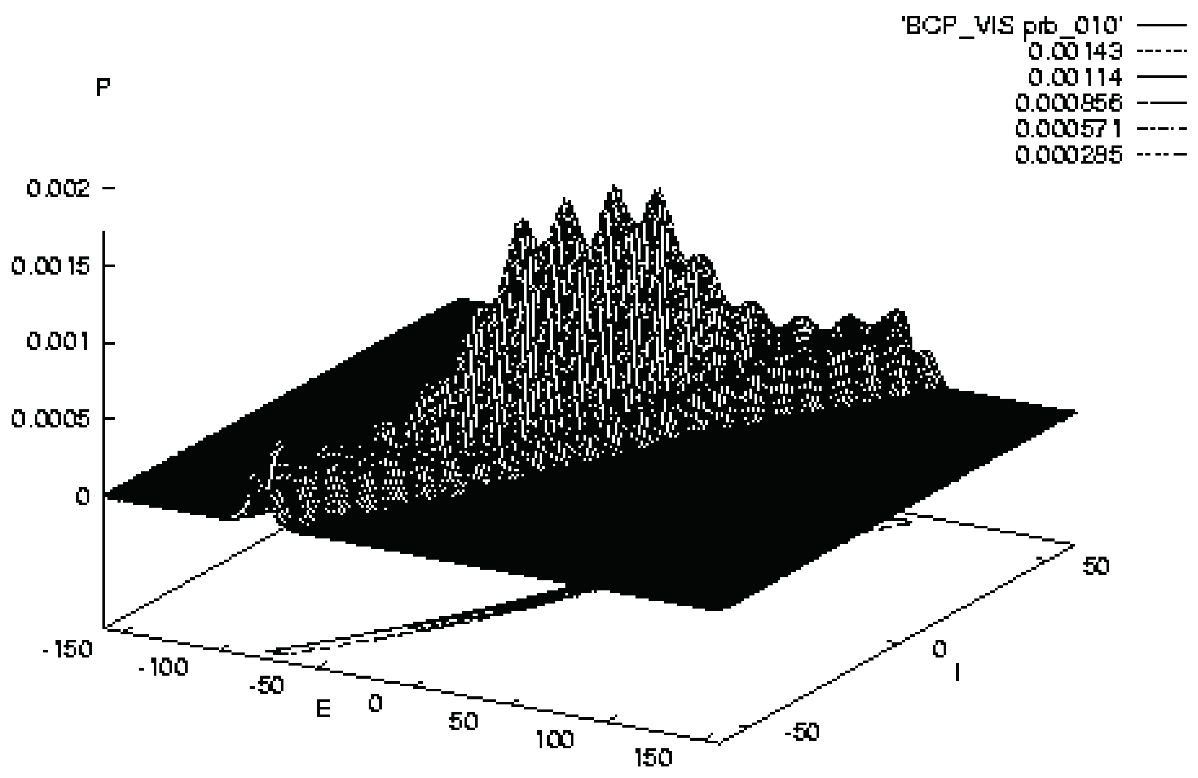
The evolution of a Balanced Centered Visual model (BCV) after 1000 foldings of , 10 unit of relaxation time , exhibits the existence of four well developed peaks. These peaks are identified with possible trappings of firing patterns. Other peaks at lower scales are clearly present, numbering on the same order as in the BC’ model, as the strength in the original peaks dissipates throughout firing space, but these are much smaller and therefore much less probable to be accessed.
2.8. Tripartite Synaptic Interactions
The human brain contains over cells, about half of which are neurons. The other half are glial cells. Astrocytes comprise a good fraction of glial cells, possibly the majority. Many papers examine the influence of astrocytes on synaptic processes [34,35,36,37,38,39,40,41,42].
http://www.astrocyte.info claims they are the most numerous cells in the human brain. Unlike the previous ideology of astrocytes being “filler” cells, they are very active in the central nervous system and greatly outnumber neurons,
Glutamate release from astrocytes through a -dependent mechanism can activate receptors at the presynaptic terminals. Intercellular calcium waves (ICWs) may travel over hundreds of astrocytes propagating over many neuronal synapses. ICWs contribute to control synaptic activity. Glutamate is released in a regenerative manner, with subsequent cells that are involved in the calcium wave releasing additional glutamate [43].
(concentrations of ) affect increased release probabilities at synaptic sites, by enhancing the release of gliotransmitters. (Free waves are considered here, not intracellular astrocyte calcium waves in situ which also increase neuronal firings.)
These free regenerative waves, arising from astrocyte-neuron interactions, couple to the magnetic vector potential produced by highly synchronous collective firings, e.g., during selective attention tasks, as measured by EEG.
2.8.1. Canonical Momentum
As derived in the Feynman (midpoint) representation of the path integral, the canonical momentum, , defines the dynamics of a moving particle with momentum in an electromagnetic field. In SI units,
where for , e is the magnitude of the charge of an electron C (Coulomb), and is the electromagnetic vector potential. (In Gaussian units , where c is the speed of light.) represents three components of a 4-vector.
2.8.2. Vector Potential of Wire
A columnar firing state is modeled as a wire/neuron with current measured in A = Amperes = C/s,
along a length z observed from a perpendicular distance r from a line of thickness . If far-field retardation effects are neglected, this yields
where is the magnetic permeability in vacuum H/m (Henry/meter). Note the insensitive log dependence on distance.
The contribution to includes minicolumnar lines of current from hundreds to thousands of macrocolumns, within a region not so large to include many convolutions, but still contributing to large synchronous bursts of EEG.
Electric and magnetic fields, derivatives of with respect to r, do not possess this logarithmic insensitivity to distance, and therefore they do not linearly accumulate strength within and across macrocolumns.
Estimates of contributions from synchronous firings to P300 measured on the scalp are tens of thousands of macrocolumns spanning 100 to 100’s of cm. Electric fields generated from a minicolumn may fall by half within 5–10 mm, the range of several macrocolumns.
There are other possible sources of magnetic vector potentials not described as wires with currents [44]. Their net effects plausibly would be included the vector magnetic potential of net synchrous firings, but not their functional forms as derived here.
2.8.3. Effects of Vector Potential on Momenta
The momentum for a ion with mass kg, speed on the order of 50 m/s to 100 m/s, is on the order of kg-m/s. Molar concentrations of waves, comprised of tens of thousands of free ions representing about 1% of a released set, most being buffered, are within a range of about 100 m to as much as 250 m, with a duration of more than 500 ms, and with [] ranging from 0.1–5 M (M = mol/m).
The magnitude of the current is taken from experimental data on dipole moments where is the direction of the current with the dipole spread over z. ranges from 1 pA-m = A-m for a pyramidal neuron [45], to A-m for larger neocortical mass [46]. These currents give rise to kg-m/s. The velocity of a wave can be ≈20–50 m/s. In neocortex, a typical wave of 1000 ions, with total mass kg times a speed of ≈20–50 m/s, gives kg-m/s.
Taking synchronous firings in a macrocolumn, leads to a dipole moment A-m. Taking z to be m m, a couple of neocortical layers, gives = kg-m/s,
2.8.4. Reasonable Estimates
Estimates used here for come from experimental data. These include shielding and material effects. When coherent activity among many macrocolumns associated with STM is considered, may be much larger. Since waves influence synaptic activity, there is direct coherence between these waves and the activity of .
Classical physics calculates from macroscopic EEG to be on the order of kg-m/s, while the momentum of a ion is on the order of kg-m/s. This numerical comparison demonstrates the possible importance of the influence of on at classical scales.
This project fits the SMNI model to EEG data. Direct calculations in classical and quantum physics support the concepts presented here, e.g., that ionic calcium momentum-wave effects among neuron-astrocyte-neuron tripartite synapses modify background SMNI parameters and create feedback between ionic/quantum and macroscopic scales [7,20,21,22,23,25,26].
2.9. Model of Models (MOM)
Deep Learning (DL) has invigorated AI approaches to parsing data in complex systems, often to develop control processes of these systems. A couple of decades ago, Neural Net AI approaches fell out of favor when concerns were apparent that such approaches offered little guidance to explain the “why” or “how” such algorithms worked to process data, e.g., contexts which were deemed important to deal with future events and outliers, etc.
The success of DL has overshadowed these concerns. However, that should not diminish their importance, especially if such systems are placed in positions to affect lives and human concerns; humans are ultimately responsible for structures they build.
An approach to dealing with these concerns can be called Model of Models (MOM). An argument in favor of MOM is that humans over thousands of years have developed models of reality across many disciplines, e.g., ranging over Physics, Biology, Mathematics, Economics, etc.
A good use of DL might be to process data for a given system in terms of a collection of models, then again use DL to process the models over the same data to determine a superior model of models (MOM). Eventually, large DL (quantum) machines could possess a database of hundreds or thousands of models across many disciplines, and directly find the best (hybrid) MOM for a given system.
In particular, SMNI offers a reasonable model upon which to further develop MOM, wherein multiple scales of observed interactions are developed. This is just one example of how physics modeling and computational physics can be used to better understand complex systems.
Ideas by Statistical Mechanics
A project sympathetic to this MOM context was proposed as Ideas by Statistical Mechanics (ISM) [47,48,49]. using ASA [50,51,52] to fit parameters of a generic nonlinear multivariate colored-noise Gaussian-Markovian short-time conditional probability distribution to data, useful for many systems.
Models developed using ASA have been applied in many contexts across many systems [53], including applications to neural networks [54].
Many of these ASA applications have used Ordinal representations of features, to permit parameterization of their inclusion into models, quite similar in spirit to DL.
ASA can be used again in the expanded context of MOM. This is suggested as a first step in a new discipline to which MOM is to be applied, to help develop a range of parameters useful for DL, as DL by itself may get stuck in non-ideal local minima of the importance-sampled space. Then, after a reasonable range of models is found, DL can take over to permit much more efficient and accurate development of MOM for a given discipline/system.
3. Adaptive Simulated Annealing (ASA) Algorithm
3.1. Importance Sampling
Nonlinear and/or stochastic systems often require importance-sampling algorithms to scan or to fit parameters. Methods of simulated annealing (SA) are often used. Proper annealing (not “quenching”) possesses a proof of finding the deepest minimum in searches.
The ASA code is open-source software, and can be downloaded and used without any cost or registration at https://www.ingber.com/#ASA [51,52].
This algorithm fits empirical data to a cost function over a D-dimensional parameter space, adapting for varying sensitivities of parameters during the fit.
This ASA algorithm is faster than fast Cauchy annealing, which has schedule , and much faster than Boltzmann annealing, which has schedule [50].
3.2. Outline of ASA Algorithm
For parameters
sampling with the random variable
the default generating function is
in terms of parameter “temperatures”
The default ASA uses the same type of annealing schedule for the acceptance function h as used for the generating function g.
All default functions in ASA can be overridden with user-defined functions.
3.3. ASA Applications
4. Path-Integral Algorithms PATHINT and qPATHINT
4.1. Path Integral in Stratonovich (Midpoint) Representation
The path integral in the Feynman (midpoint) representation is used to examine discretization issues in time-dependent nonlinear systems [75,76,77]. (N.b. in implies a prepoint evaluation.) Unless explicitly stated, the Einstein summation convention is used which implies repeated indices signify summation; bars imply no summation.
Non-constant diffusions add terms to drifts, and a Riemannian-curvature potential is induced for dimension in the Stratonovich/Feynman discretization.
4.2. Path Integral in Ito (Prepoint) Representation
In the Ito (prepoint) representation:
Here the diagonal diffusions are and the drifts are .
4.3. Path-Integral Riemannian Geometry
The midpoint derivation derives a Riemannian geometry with metric defined by the inverse of the covariance matrix
and where R is the Riemannian curvature
An Ito prepoint discretization for the same probability distribution P gives a simpler algebraic form,
but the Lagrangian L so specified does not satisfy a variational principle useful for moderate to large noise. Its variational principle is only useful in the weak-noise limit. This often means that finer meshes are required.
4.4. Three Approaches Are Mathematically Equivalent
Three basic different approaches are mathematically equivalent:
- (a)
- Fokker-Planck/Chapman-Kolmogorov partial-differential equations
- (b)
- Langevin coupled stochastic-differential equations
- (c)
- Lagrangian or Hamiltonian path-integrals
All three are described here as many researchers are familiar with at least one of these approaches to complex systems.
The path-integral approach is useful to define intuitive physical variables from the Lagrangian L in terms of underlying variables :
Differentiation especially of noisy systems often introduces more noise. The path-integral often gives superior numerical performance because integration is a smoothing process.
4.4.1. Stochastic Differential Equation (SDE)
The Stratonovich (midpoint discretized) Langevin equations can be analyzed in terms of the Wiener process . This can be developed with Gaussian noise , with some care taken in the limit of small .
represents Gaussian white noise.
4.4.2. Partial Differential Equation (PDE)
The Fokker-Planck, sometimes defines as Chapman-Kolmogorov, partial differential equation is:
replaces in the SDE if the Ito (prepoint discretized) calculus is used. If boundary conditions are added as Lagrange multipliers, these enter as a “potential” V creating a Schrodinger-type equation.
4.5. PATHINT Applications
4.6. PATHINT/qPATHINT Code
qPATHINT is an N-dimensional code developed to calculate the propagation of quantum variables in the presence of shocks. Many real systems propagate in the presence of sudden changes of state dependent on time. qPATHINT is based on the classical-physics code, PATHINT, which has been useful in several systems across several disciplines. Applications have been made to SMNI and Statistical Mechanics of Financal Markets (SMFM) [23,24,80].
To numerically calculate the path integral for serial changes in time, standard Monte Carlo techniques generally are not useful. PATHINT was originally developed for this purpose. The PATHINT C code of about 7500 lines of code using the GCC C-compiler was rewritten to use double complex variables instead of double variables, and further developed for arbitrary N dimensions, creating qPATHINT. The outline of the code is described here for classical or quantum systems, using generic coordinates q [23,79,80]:
The distribution (probabilities for classical systems, wave-functions for quantum systems) can be numerically approximated to a high degree of accuracy using a histogram procedure, developing sums of rectangles of height and width at points .
4.6.1. Shocks
Many real-world systems propagate in the presence of continual “shocks”.
In SMNI, collisions occur via regenerative waves. There also are interactions with changing due to changing highly synchronous neuronal firings.
In SMFM applications, shocks occur due to future dividends, changes in interest rates, changes in asset distributions, etc.
4.6.2. PATHINT/qPATHINT Histograms
A one-dimensional path-integral in variable q in the prepoint Ito discretization is developed in terms of the kernel/propagator G, for each of its intermediate integrals, as
This yields
is a banded matrix representing the Gaussian nature of the short-time probability centered about the drift.
4.6.3. Meshes For [q]PATHINT
Explicit dependence of L on time t can be included. The mesh is strongly dependent on diagonal elements of the diffusion matrix, e.g.,
This constrains the dependence of the covariance of each variable to be a (nonlinear) function of that variable to present a rectangular underlying mesh. Since integration is inherently a smoothing process [58], coarser meshes are used relative to the corresponding stochastic differential equation(s) [84].
By considering the contributions to the first and second moments, conditions on the time and variable meshes can be derived. Thus can be measured by the diffusion divided by the square of the drift.
4.7. Lessons Learned From SMFM and SMNI
SMNI qPATHINT has emphasized the requirement of broad-banded kernels for oscillatory quantum states.
SMFM PATHTREE, and its derived qPATHTREE, is a different options code, based on path-integral error analyses, permitting a new very fast binary calculation, also applied to nonlinear time-dependent systems [62]. However, in contrast to the present PATHINT/qPATHINT code that has been generalized to N dimensions, currently an SMFM [q]PATHTREE is only a binary tree with and cannot be effectively applied to quantum oscillatory systems [23,79,80].
Calculations At Each Node At Each Time Slice
SMFM [q]PATHINT for (American) financial options: Calculate at each node of each time slice—back in time.
SMNI [q]PATHINT: Calculate at each node of each time slice—forward in time.
At each node of each time slice, a proposed algorithm is to calculate quantum-scale wave-packet (2-way) interactions with macroscopic large-scale EEG/. This entails algorithms:
- PATHINT using the Classical SMNI Lagrangian
- qPATHINT using the Quantum wave-packet Lagrangian
- Sync in time during P300 attentional tasks.
- Time/phase relations between classical and quantum systems may be important.
- ASA-fit synchronized classical-quantum PATHINT-qPATHINT model to EEG data.
- is determined experimentally from EEG, and includes all synaptic background effects.
5. Results Including Quantum Scales
The wave function describing the interaction of with of wave packets was derived in closed form from the Feynman representation of the path integral using path-integral techniques [87], modified here to include .
where is the initial Gaussian packet, is the free-wave evolution operator, ℏ is the Planck constant, q is the electronic charge of ions, m is the mass of a wave-packet of 1000 ions, is the spatial variance of the wave-packet, the initial momentum is , and the evolving canonical momentum is . Detailed calculations show that of the wave packet and of the EEG field make about equal contributions to .
5.1. SMNI + Wave-Packet
Tripartite influence on synaptic is measured by the ratio of packet’s to at the onset of each attentional task. Here is taken over .
changes slower than , so static approximation of used to derive and is reasonable to use within P300 EEG epochs, resetting at the onset of each classical EEG measurement (1.953 ms apart), using the current . This permits tests of interactions across scales in a classical context.
5.2. Supercomputer Resources
The XSEDE.org University of California San Diego (UCSD) supercomputer resource is Comet, described at https://portal.xsede.org/sdsc-comet.
About 1000 h of supercomputer CPUs are required for an ASA fit of SMNI to the same EEG data used previously, i.e., from http://physionet.nlm.nih.gov/pn4/erpbci [31,32], using mostly the same codes used previously [22]. Many such sets of runs are required. Including quantum processes will take even longer.
5.3. Results Using
was used in classical-physics SMNI fits to EEG data using ASA. Runs using 1M or 100K generated states gave results not much different. Training with ASA used 100K generated states over 12 subjects with and without , followed by 1000 generated states with the simplex local code contained with ASA. Training and Testing runs on XSEDE.org for this project has taken an equivalent of several months of CPU on the XSEDE.org UCSD platform Comet. These calculations use one additional parameter across all EEG regions to weight the contribution to synaptic background . is taken to be proportional to the currents measured by EEG, i.e., firings . Otherwise, the “zero-fit-parameter” SMNI philosophy was enforced, wherein parameters are picked from experimentally determined values or within experimentally determined ranges [4].
As with previous studies using this data, results sometimes give Testing cost functions less than the Training cost functions. This reflects on great differences in data, likely from great differences in subjects’ contexts, e.g., possibly due to subjects’ STM strategies only sometimes including effects calculated here. Further tests of these multiple-scale models with more EEG data are required, and with the PATHINT-qPATHINT coupled algorithm described previously.
Table 1 gives recent results on such tests. Cost functions are the effective Action, , which is , where the prefactor multiplier of the exponential arises from the normalization of the short-time conditional probability distribution and is the argument of the exponential factor. Equation (3) defines the Lagrangian L, and the normalization is defined in in Equation (11).
5.4. Quantum Zeno Effects
The quantum-mechanical wave function of the wave packet was shown to “survive” overlaps after multiple collisions, due to their regenerative processes during the observed long durations of hundreds of ms. Thus, waves may support a Zeno or “bang-bang” effect which may promote long coherence times [88,89,90,91,92,93,94,95,96].
Of course, the Zeno/“bang-bang” effect may exist only in special contexts, since decoherence among particles is known to be very fast, e.g., faster than phase-damping of macroscopic classical particles colliding with quantum particles [97].
The wave may be perpetuated by the constant collisions of ions as they enter and leave the wave packet due to the regenerative collisions by the Zeno/“bang-bang” effect. qPATHINT can calculate the coherence stability of the wave due to serial shocks.
Survival of Wave Packet
In momentum space, the wave packet is considered as being “kicked” from to . Assume that random repeated kicks of result in , and that each kick keeps the variance . Then, the overlap integral at the moment t of a typical kick between the new and old state is
where is the normalized wave function in momentum space. A crude estimate is obtained of the survival time amplitude and survival probability [90],
These numbers yield:
Even many small repeated kicks do not appreciably affect the real part of , and these projections do not appreciably destroy the original wave packet, giving a survival probability per kick as .
The time-dependent phase terms are sensitive to times of tenths of a sec. These times are prominent in STM and in synchronous neural firings. Therefore, effects on wave functions may maximize their influence on STM at frequencies consistent with synchronous EEG during STM.
6. Quantum Applications
6.1. Nano-Robotic Applications
There is the possibility of carrying pharmaceutical products in nanosystems that could affect unbuffered waves in neocortex [21]. A -wave momentum-sensor could act like a piezoelectric device.
At the onset of a wave (on the order of 100’s of ms), a change of momentum can be on the order of kg-m/s for a typical ion. A wave packet of 1000 ions with onset time of 1 ms, exerts a force on the order of N (1 N ≡ 1 Newton = 1 kg-m/s). A nano-robot would be attracted to this site, depositing chemicals/drugs that interact with the regenerative -wave process.
An area of the receptor of the nanosystem of 1 nm would require pressure sensitivity of Pa (1 Pa = 1 pascal = 1 N/m).
The nano-roboot could be switched on/off at a regional/columnar level by sensitivity to local electric/magnetic fields. Highly synchronous firings during STM processes can be affected by these piezoelectric nanosystems which affect background/noise efficacies via control of waves. In turn, this would affect the influence of of waves via the vector potential , etc.
6.2. Free Will
There is interest in researching possible quantum influences on highly synchronous neuronal firings relevant to STM to understand connections to consciousness and “Free Will” (FW) [22,79].
If experimental evidence is gained of quantum-level processes of tripartite synaptic interactions with large-scale synchronous neuronal firings, then FW may be established using the Conway-Kochen quantum no-clone “Free Will Theorem” (FWT) [101,102].
The essence of FWT is that, since quantum states cannot be cloned, a quantum wave-packet may not generate a state proven to have previously existed. As explained by the authors [101,102], experimenters have specific choices in selecting measurements, which are shared by (twinned) particles, including the choice of any random number generator that might be used to aid such choices. The authors maintain that their proof and description of quantum measurements used is general enough to rule out classical randomness, and that classical determinism cannot be supported by such processes as exist in the quantum world.
7. Conclusions
The SMNI model has demonstrated it is faithful to experimental data, for EEG recordings under STM experimental paradigms. qPATHINT permits an inclusion of quantum scales in the multiple-scale SMNI model, by evolving wave-packets with momentum , including serial shocks, interacting with the magnetic vector potential derived from EEG data, marching forward in time lock-step with experimental EEG data. This presents a time-dependent propagation of interacting quantum and classical scales.
This quantum path-integral algorithm with serial random shocks will be further studied as it can be used for many quantum systems.
Funding
The author thanks the Extreme Science and Engineering Discovery Environment (XSEDE.org), for supercomputer grants since February 2013, starting with Electroencephalographic field influence on calcium momentum waves, one under PHY130022 and two under TG-MCB140110. The current grant under TG-MCB140110, Quantum path-integral qPATHTREE and qPATHINT algorithms, was started in 2017, and renewed through December 2018.
Acknowledgments
The author thanks the Extreme Science and Engineering Discovery Environment (XSEDE.org), for supercomputer grants since February 2013, starting with “Electroencephalographic field influence on calcium momentum waves”, one under PHY130022 and two under TG-MCB140110. The current grant under TG-MCB140110, “Quantum path-integral qPATHTREE and qPATHINT algorithms”, was started in 2017, and renewed through December 2018. XSEDE grants have spanned several projects described in https://www.ingber.com/lir_computational_physics_group.html.
Conflicts of Interest
The author declares no conflict of interest.
References
- Ingber, L. Towards a unified brain theory. J. Soc. Biol. Struct. 1981, 4, 211–224. [Google Scholar] [CrossRef]
- Ingber, L. Statistical mechanics of neocortical interactions. I. Basic formulation. Phys. D 1982, 5, 83–107. [Google Scholar] [CrossRef]
- Ingber, L. Statistical mechanics of neocortical interactions. Dynamics of synaptic modification. Phys. Rev. A 1983, 28, 395–416. [Google Scholar] [CrossRef]
- Ingber, L. Statistical mechanics of neocortical interactions. Derivation of short-term-memory capacity. Phys. Rev. A 1984, 29, 3346–3358. [Google Scholar] [CrossRef]
- Ingber, L. Statistical mechanics of neocortical interactions: Stability and duration of the 7+−2 rule of short-term-memory capacity. Phys. Rev. A 1985, 31, 1183–1186. [Google Scholar] [CrossRef]
- Ingber, L. Statistical mechanics of neocortical interactions: Path-integral evolution of short-term memory. Phys. Rev. E 1994, 49, 4652–4664. [Google Scholar] [CrossRef]
- Ingber, L. Columnar EEG magnetic influences on molecular development of short-term memory. In Short-Term Memory: New Research; Kalivas, G., Petralia, S., Eds.; Nova: Hauppauge, NY, USA, 2012; pp. 37–72. [Google Scholar]
- Ericsson, K.; Chase, W. Exceptional memory. Am. Sci. 1982, 70, 607–615. [Google Scholar]
- Zhang, G.; Simon, H. STM capacity for Chinese words and idioms: Chunking and acoustical loop hypotheses. Mem. Cognit. 1985, 13, 193–201. [Google Scholar] [CrossRef] [PubMed]
- Hick, W. On the rate of gains of information. Q. J. Exp. Psychol. 1952, 34, 1–33. [Google Scholar] [CrossRef]
- Ingber, L. Statistical mechanics of neocortical interactions: Reaction time correlates of the g factor. Psycholoquy 1999, 10. Article Number 35. [Google Scholar]
- Jensen, A. Individual differences in the Hick paradigm. In Speed of Information-Processing and Intelligence; Vernon, P., Ed.; Ablex: Norwood, NJ, USA, 1987; pp. 101–175. [Google Scholar]
- Ingber, L. Statistical mechanics of neocortical interactions: Applications of canonical momenta indicators to electroencephalography. Phys. Rev. E 1997, 55, 4578–4593. [Google Scholar] [CrossRef]
- Ingber, L. EEG Database; UCI Machine Learning Repository: Irvine, CA, USA, 1997. [Google Scholar]
- Ingber, L. Statistical mechanics of multiple scales of neocortical interactions. In Neocortical Dynamics and Human EEG Rhythms; Nunez, P., Ed.; Oxford University Press: New York, NY, USA, 1995; pp. 628–681. ISBN 0-19-505728-7. [Google Scholar]
- Asher, J. Brain’s Code for Visual Working Memory Deciphered in Monkeys NIH-Funded Study; Technical Report NIH Press Release; NIH, Bethesda: Rockville, MD, USA, 2012. [Google Scholar]
- Salazar, R.; Dotson, N.; Bressler, S.; Gray, C. Content-specific fronto-parietal synchronization during visual working memory. Science 2012, 338, 1097–1100. [Google Scholar] [CrossRef]
- Ingber, L. Statistical mechanics of neocortical interactions: Constraints on 40 Hz models of short-term memory. Phys. Rev. E 1995, 52, 4561–4563. [Google Scholar] [CrossRef]
- Ingber, L. Computational algorithms derived from multiple scales of neocortical processing. In Pointing at Boundaries: Integrating Computation and Cognition on Biological Grounds; Pereira, A., Jr., Massad, E., Bobbitt, N., Eds.; Springer: New York, NY, USA, 2011; pp. 1–13. [Google Scholar]
- Ingber, L. Influence of macrocolumnar EEG on Ca waves. Curr. Prog. J. 2012, 1, 4–8. [Google Scholar] [CrossRef]
- Ingber, L. Calculating consciousness correlates at multiple scales of neocortical interactions. In Horizons in Neuroscience Research; Costa, A., Villalba, E., Eds.; Nova: Hauppauge, NY, USA, 2015; pp. 153–186. ISBN 978-1-63482-632-7. [Google Scholar]
- Ingber, L. Statistical mechanics of neocortical interactions: Large-scale EEG influences on molecular processes. J. Theor. Biol. 2016, 395, 144–152. [Google Scholar] [CrossRef]
- Ingber, L. Evolution of regenerative Ca-ion wave-packet in neuronal-firing fields: Quantum path-integral with serial shocks. Int. J. Innov. Res. Inf. Secur. 2017, 4, 14–22. [Google Scholar] [CrossRef]
- Ingber, L. Quantum Path-Integral qPATHINT Algorithm. Open Cybern. Syst. J. 2017, 11, 119–133. [Google Scholar] [CrossRef]
- Ingber, L.; Pappalepore, M.; Stesiak, R. Electroencephalographic field influence on calcium momentum waves. J. Theor. Biol. 2014, 343, 138–153. [Google Scholar] [CrossRef]
- Nunez, P.; Srinivasan, R.; Ingber, L. Theoretical and experimental electrophysiology in human neocortex: Multiscale correlates of conscious experience. In Multiscale Analysis and Nonlinear Dynamics: From Genes to the Brain; Pesenson, M., Ed.; Wiley: New York, NY, USA, 2013; pp. 149–178. [Google Scholar] [CrossRef]
- Ingber, L. Towards clinical applications of statistical mechanics of neocortical interactions. Innov. Technol. Biol. Med. 1985, 6, 753–758. [Google Scholar]
- Ingber, L. Statistical mechanics of neocortical interactions. EEG dispersion relations. IEEE Trans. Biomed. Eng. 1985, 32, 91–94. [Google Scholar] [CrossRef] [PubMed]
- Briggs, F.; Mangun, G.; Usrey, W. Attention enhances synaptic efficacy and the signal-to-noise ratio in neural circuits. Nature 2013, 499, 1–5. [Google Scholar] [CrossRef] [PubMed]
- Mountcastle, V.; Andersen, R.; Motter, B. The influence of attentive fixation upon the excitability of the light-sensitive neurons of the posterior parietal cortex. J. Neurosci. 1981, 1, 1218–1235. [Google Scholar] [CrossRef] [PubMed]
- Citi, L.; Poli, R.; Cinel, C. Documenting, modelling and exploiting P300 amplitude changes due to variable target delays in Donchin’s speller. J. Neural Eng. 2010, 7, 1–21. [Google Scholar] [CrossRef]
- Goldberger, A.; Amaral, L.; Glass, L.; Hausdorff, J.; Ivanov, P.; Mark, R.; Mietus, J.; Moody, G.; Peng, C.K.; Stanley, H. PhysioBank, PhysioToolkit, and PhysioNet: Components of a New Research Resource for Complex Physiologic Signals. Circulation 2000, 101, e215–e220. [Google Scholar] [CrossRef]
- Ingber, L.; Nunez, P. Statistical mechanics of neocortical interactions: High resolution path-integral calculation of short-term memory. Phys. Rev. E 1995, 51, 5074–5083. [Google Scholar] [CrossRef]
- Agulhon, C.; Petravicz, J.; McMullen, A.; Sweger, E.; Minton, S.; Taves, S.; Casper, K.; Fiacco, T.; McCarthy, K. What is the role of astrocyte calcium in neurophysiology? Neuron 2008, 59, 932–946. [Google Scholar] [CrossRef] [PubMed]
- Araque, A.; Navarrete, M. Glial cells in neuronal network function. Phil. Trans. R. Soc. B-Boil. Sci. 2010, 365, 2375–2381. [Google Scholar] [CrossRef]
- Banaclocha, M.; Bookkon, I.; Banaclocha, H. Long-term memory in brain magnetite. Med. Hypotheses 2010, 74, 254–257. [Google Scholar] [CrossRef]
- Bellinger, S. Modeling calcium wave oscillations in astrocytes. Neurocomputing 2005, 65, 843–850. [Google Scholar] [CrossRef]
- Innocenti, B.; Parpura, V.; Haydon, P. Imaging extracellular waves of glutamate during calcium signaling in cultured astrocytes. J. Neurosci. 2000, 20, 1800–1808. [Google Scholar] [CrossRef]
- Pereira, A.; Furlan, F.A. On the role of synchrony for neuron-astrocyte interactions and perceptual conscious processing. J. Biol. Phys. 2009, 35, 465–480. [Google Scholar] [CrossRef]
- Reyes, R.; Parpura, V. The trinity of Ca2+ sources for the exocytotic glutamate release from astrocytes. Neurochem. Int. 2009, 55, 1–14. [Google Scholar] [CrossRef] [PubMed]
- Scemes, E.; Giaume, C. Astrocyte calcium waves: What they are and what they do. Glia 2006, 54, 716–725. [Google Scholar] [CrossRef]
- Volterra, A.; Liaudet, N.; Savtchouk, I. Astrocyte Ca2+ signalling: An unexpected complexity. Nat. Rev. Neurosci. 2014, 15, 327–335. [Google Scholar] [CrossRef] [PubMed]
- Ross, W. Understanding calcium waves and sparks in central neurons. Nat. Rev. Neurosci. 2012, 13, 157–168. [Google Scholar] [CrossRef] [PubMed]
- Majhi, S.; Ghosh, D. Alternating chimeras in networks of ephaptically coupled bursting neurons. Chaos 2018, 28. [Google Scholar] [CrossRef]
- Murakami, S.; Okada, Y. Contributions of principal neocortical neurons to magnetoencephalography and electroencephalography signals. J. Physiol. 2006, 575, 925–936. [Google Scholar] [CrossRef]
- Nunez, P.; Srinivasan, R. Electric Fields of the Brain: The Neurophysics of EEG, 2nd ed.; Oxford University Press: London, UK, 2006. [Google Scholar]
- Ingber, L. Ideas by Statistical Mechanics (ISM); Technical Report Report 2006:ISM, Lester Ingber Research; Ashland: Covington, OR, USA, 2006. [Google Scholar]
- Ingber, L. Ideas by Statistical Mechanics (ISM). J. Integr. Syst. Des. Process Sci. 2007, 11, 31–54. [Google Scholar] [CrossRef]
- Ingber, L. AI and Ideas by Statistical Mechanics (ISM). In Encyclopedia of Artificial Intelligence; Rabunal, J., Dorado, J., Pazos, A., Eds.; Information Science Reference: New York, NY, USA, 2008; pp. 58–64. ISBN 978-1-59904-849-9. [Google Scholar]
- Ingber, L. Very fast simulated re-annealing. Math. Comput. Model. 1989, 12, 967–973. [Google Scholar] [CrossRef]
- Ingber, L. Adaptive Simulated Annealing (ASA); Technical Report Global optimization C-code; Caltech Alumni Association: Pasadena, CA, USA, 1993. [Google Scholar]
- Ingber, L. Adaptive Simulated Annealing. In Stochastic Global Optimization and Its Applications with Fuzzy Adaptive Simulated Annealing; Oliveira, H.A., Petraglia, A., Ingber, L., Machado, M., Petraglia, M., Eds.; Springer: New York, NY, USA, 2012; pp. 33–61. [Google Scholar]
- Ingber, L. Simulated annealing: Practice versus theory. Math. Comput. Model. 1993, 18, 29–57. [Google Scholar] [CrossRef]
- Atiya, A.; Parlos, A.; Ingber, L. A reinforcement learning method based on adaptive simulated annealing. In Proceedings International Midwest Symposium on Circuits and Systems (MWCAS), December 2003; IEEE CAS: Cairo, Egypt, 2003. [Google Scholar]
- Ingber, L.; Srinivasan, R.; Nunez, P. Path-integral evolution of chaos embedded in noise: Duffing neocortical analog. Math. Comput. Model. 1996, 23, 43–53. [Google Scholar] [CrossRef]
- Ingber, L. Statistical mechanics of combat and extensions. In Toward a Science of Command, Control, and Communications; Jones, C., Ed.; American Institute of Aeronautics and Astronautics: Washington, DC, USA, 1993; pp. 117–149. ISBN 1-56347-068-3. [Google Scholar]
- Ingber, L. Data mining and knowledge discovery via statistical mechanics in nonlinear stochastic systems. Math. Comput. Model. 1998, 27, 9–31. [Google Scholar] [CrossRef]
- Ingber, L. Statistical mechanical aids to calculating term structure models. Phys. Rev. A 1990, 42, 7057–7064. [Google Scholar] [CrossRef]
- Ingber, L. Canonical momenta indicators of financial markets and neocortical EEG. In Progress in Neural Information Processing, Proceedings of the 1996 International Conference on Neural Information Processing (ICONIP’96), Hong Kong, 24–27 September 1996; Amari, S.I., Xu, L., King, I., Leung, K.S., Eds.; Springer: New York, NY, USA, 1996; pp. 777–784. [Google Scholar]
- Ingber, L. High-resolution path-integral development of financial options. Phys. A 2000, 283, 529–558. [Google Scholar] [CrossRef]
- Ingber, L. Trading in Risk Dimensions (TRD); Technical Report Report 2005:TRD, Lester Ingber Research; Ashland: Covington, OR, USA, 2005. [Google Scholar]
- Ingber, L.; Chen, C.; Mondescu, R.; Muzzall, D.; Renedo, M. Probability tree algorithm for general diffusion processes. Phys. Rev. E 2001, 64, 056702–056707. [Google Scholar] [CrossRef]
- Ingber, L.; Mondescu, R. Automated internet trading based on optimized physics models of markets. In Intelligent Internet-Based Information Processing Systems; Howlett, R., Ichalkaranje, N., Jain, L., Tonfoni, G., Eds.; World Scientific: Singapore, 2003; pp. 305–356. [Google Scholar]
- Ingber, L. Statistical mechanics of neocortical interactions: A scaling paradigm applied to electroencephalography. Phys. Rev. A 1991, 44, 4017–4060. [Google Scholar] [CrossRef]
- Ingber, L. Generic mesoscopic neural networks based on statistical mechanics of neocortical interactions. Phys. Rev. A 1992, 45, R2183–R2186. [Google Scholar] [CrossRef]
- Ingber, L. Statistical mechanics of neocortical interactions: Multiple scales of EEG. In Frontier Science in EEG: Continuous Waveform Analysis (Electroencephal. clin. Neurophysiol. Suppl. 45); Dasheiff, R., Vincent, D., Eds.; Elsevier: Amsterdam, The Netherlands, 1996; pp. 79–112. ISBN 0-444-82429-4. [Google Scholar]
- Ingber, L. Statistical mechanics of neocortical interactions: Training and testing canonical momenta indicators of EEG. Math. Comput. Model. 1998, 27, 33–64. [Google Scholar] [CrossRef]
- Ingber, L. Statistical Mechanics of Neocortical Interactions: Portfolio of Physiological Indicators; Technical Report Report 2006:PPI, Lester Ingber Research; Ashland: Covington, OR, USA, 2006. [Google Scholar]
- Ingber, L. Statistical mechanics of neocortical interactions: Portfolio of physiological indicators. Open Cybern. Syst. J. 2009, 3, 13–26. [Google Scholar] [CrossRef]
- Ingber, L. Statistical mechanics of neocortical interactions: Nonlinear columnar electroencephalography. NeuroQuantology J. 2009, 7, 500–529. [Google Scholar]
- Ingber, L. Electroencephalographic (EEG) Influence on Ca2+ Waves: Lecture Plates; Technical Report Report 2013:LEFI, Lester Ingber Research; Ashland: Covington, OR, USA, 2013. [Google Scholar]
- Ingber, L.; Nunez, P. Neocortical Dynamics at Multiple Scales: EEG Standing Waves, Statistical Mechanics, and Physical Analogs. Math. Biosci. 2010, 229, 160–173. [Google Scholar] [CrossRef] [PubMed]
- Ingber, L. Adaptive simulated annealing (ASA): Lessons learned. Control Cybern. 1996, 25, 33–54. [Google Scholar]
- Ingber, L.; Rosen, B. Genetic algorithms and very fast simulated reannealing: A comparison. Math. Comput. Model. 1992, 16, 87–100. [Google Scholar] [CrossRef]
- Langouche, F.; Roekaerts, D.; Tirapegui, E. Discretization problems of functional integrals in phase space. Phys. Rev. D 1979, 20, 419–432. [Google Scholar] [CrossRef]
- Langouche, F.; Roekaerts, D.; Tirapegui, E. Functional Integration and Semiclassical Expansions; Reidel: Dordrecht, The Netherlands, 1982. [Google Scholar]
- Schulman, L. Techniques and Applications of Path Integration; J. Wiley Sons: New York, NY, USA, 1981. [Google Scholar]
- Ingber, L.; Fujio, H.; Wehner, M. Mathematical comparison of combat computer models to exercise data. Math. Comput. Model. 1991, 15, 65–90. [Google Scholar] [CrossRef]
- Ingber, L. Path-integral quantum PATHTREE and PATHINT algorithms. Int. J. Innov. Res. Inf. Secur. 2016, 3, 1–15. [Google Scholar] [CrossRef]
- Ingber, L. Options on quantum money: Quantum path-integral with serial shocks. Int. J. Innov. Res. Inf. Secur. 2017, 4, 7–13. [Google Scholar] [CrossRef]
- Ingber, L.; Wilson, J. Statistical mechanics of financial markets: Exponential modifications to Black-Scholes. Math. Comput. Model. 2000, 31, 167–192. [Google Scholar] [CrossRef]
- Ingber, L. Path-integral evolution of multivariate systems with moderate noise. Phys. Rev. E 1995, 51, 1616–1619. [Google Scholar] [CrossRef]
- Ingber, L.; Wilson, J. Volatility of volatility of financial markets. Math. Comput. Model. 1999, 29, 39–57. [Google Scholar] [CrossRef]
- Wehner, M.; Wolfer, W. Numerical evaluation of path-integral solutions to Fokker-Planck equations. I. Phys. Rev. A 1983, 27, 2663–2670. [Google Scholar] [CrossRef]
- Wehner, M.; Wolfer, W. Numerical evaluation of path-integral solutions to Fokker-Planck equations. II. Restricted stochastic processes. Phys. Rev. A 1983, 28, 3003–3011. [Google Scholar] [CrossRef]
- Wehner, M.; Wolfer, W. Numerical evaluation of path integral solutions to Fokker-Planck equations. III. Time and functionally dependent coefficients. Phys. Rev. A 1987, 35, 1795–1801. [Google Scholar] [CrossRef]
- Schulten, K. Quantum Mechanics; Technical Report PHYS480 Lecture Notes, Chapter 2. Available online: http://www.ks.uiuc.edu/Services/Class/PHYS480/ (accessed on 29 November 2018).
- Burgarth, D.; Facchi, P.; Nakazato, H.; Pascazio, S.; Yuasa, K. Quantum Zeno Dynamics from General Quantum Operations. arXiv, 2018; arXiv:1809.09570. [Google Scholar]
- Facchi, P.; Lidar, D.; Pascazio, S. Unification of dynamical decoupling and the quantum Zeno effect. Phys. Rev. A 2004, 69, 1–6. [Google Scholar] [CrossRef]
- Facchi, P.; Pascazio, S. Quantum Zeno dynamics: Mathematical and physical aspects. J. Phys. A 2008, 41, 1–45. [Google Scholar] [CrossRef]
- Giacosa, G.; Pagliara, G. Quantum Zeno effect by general measurements. Phys. Rev. A 2014, 052107, 1–5. [Google Scholar]
- Kozlowski, W.; Caballero-Benitez, S.; Mekhov, I. Non-Hermitian Dynamics in the Quantum Zeno Limit. arXiv, 2018; arXiv:1510.04857. [Google Scholar] [CrossRef]
- Muller, M.; Gherardini, S.; Caruso, F. Quantum Zeno Dynamics through Stochastic Protocols. arXiv, 2018; arXiv:1607.08871v1. [Google Scholar] [CrossRef]
- Patil, Y.; Chakram, S.; Vengalattore, M. Measurement-induced localization of an ultracold lattice gas. Phys. Rev. Lett. 2015, 115, 1–5. [Google Scholar] [CrossRef]
- Wu, S.; Wang, L.; Yi, X. Time-dependent decoherence-free subspace. J. Phys. A 2012, 405305, 1–11. [Google Scholar] [CrossRef]
- Zhang, P.; Ai, Q.; Li, Y.; Xu, D.; Sun, C. Dynamics of quantum Zeno and anti-Zeno effects in an open system. Sci. China Phys. Mech. Astron. 2014, 57, 194–207. [Google Scholar] [CrossRef]
- Preskill, J. Quantum Mechanics; Technical Report Lecture Notes; Caltech: Pasadena, CA, USA, 2015. [Google Scholar]
- Hagan, S.; Hameroff, S.; Tuszynski, J. Quantum computation in brain microtubules: Decoherence and biological feasibility. Phys. Rev. E 2002, 65, 1–11. [Google Scholar] [CrossRef] [PubMed]
- Hameroff, S.; Penrose, R. Consciousness in the universe: A review of the ‘Orch OR’ theory. Phys. Life Rev. 2013, 403, 1–40. [Google Scholar] [CrossRef]
- McKemmish, L.; Reimers, J.; McKenzie, R.; Mark, A.; Hush, N. Penrose-Hameroff orchestrated objective-reduction proposal for human consciousness is not biologically feasible. Phys. Rev. E 2009, 80, 1–6. [Google Scholar] [CrossRef] [PubMed]
- Conway, J.; Kochen, S. The free will theorem. Found. Phys. 2006, 36, 1441–1473. [Google Scholar] [CrossRef]
- Conway, J.; Kochen, S. The strong free will theorem. Notices Am. Math. Soc. 2009, 56, 226–232. [Google Scholar]
Figure 1.
Illustrates three SMNI biophysical scales [2,3]: (a)-(a)-(a’) microscopic neurons; (b)-(b’) mesocolumnar domains; (c)-(c’) macroscopic regions; (a): synaptic inter-neuronal interactions, scaled up to mesocolumns, phenomenologically described by the mean and variance of a distribution . (a): intraneuronal transmissions phenomenologically described by the mean and variance of . (a’): collective mesocolumnar-averaged inhibitory (I) and excitatory (E) neuronal firings M; (b): vertical organization of minicolumns including their horizontal layers, yielding a physiological entity, the mesocolumn (b’): overlapping mesocolumns at locations r and from times t and , on the order of 10 ms; (c): macroscopic regions of neocortex arising from many mesocolumnar domains (c’): regions coupled by long-ranged interactions.
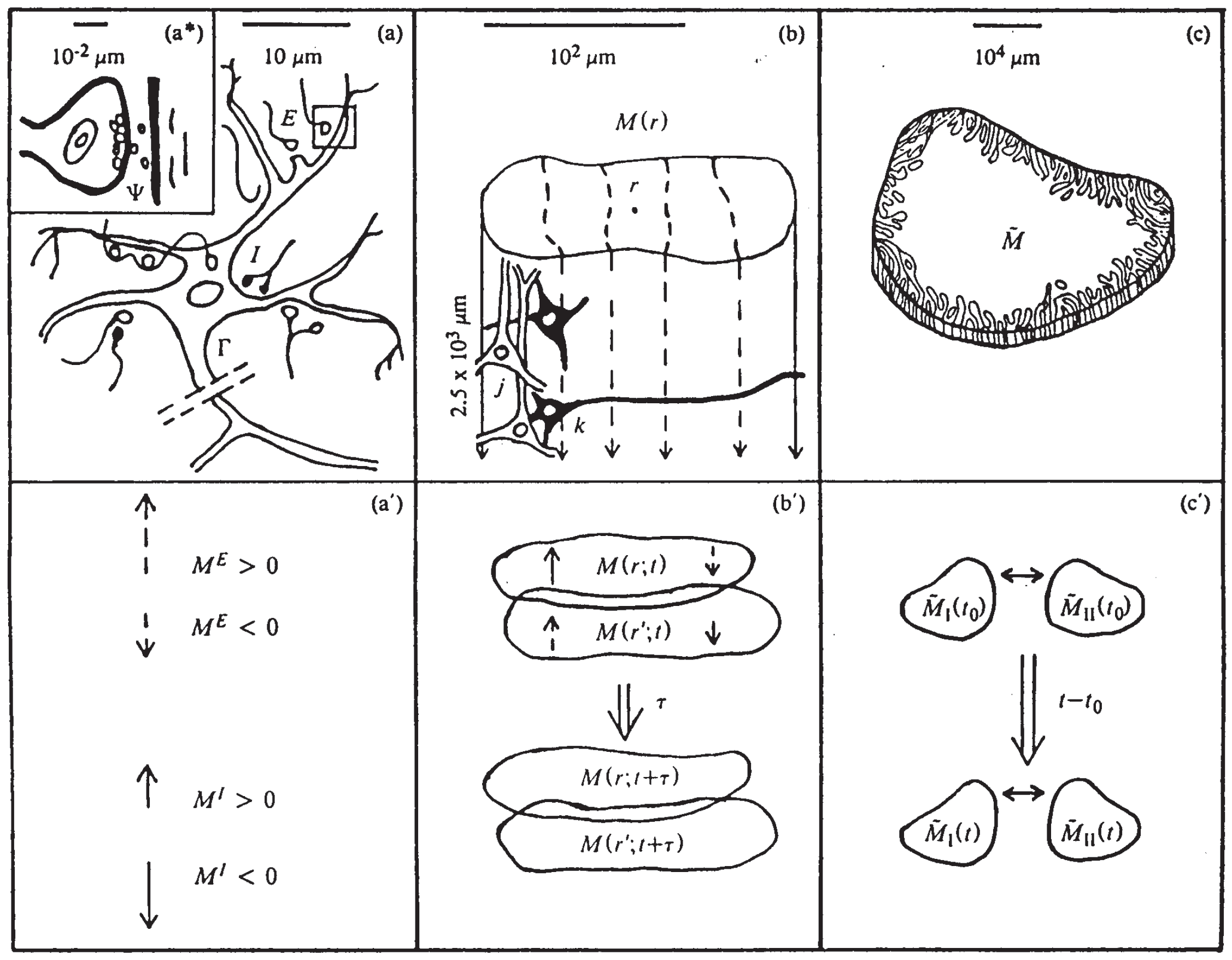
Figure 2.
Illustrates SMNI STM Model BC at the evolution at 5 [33].
Figure 2.
Illustrates SMNI STM Model BC at the evolution at 5 [33].
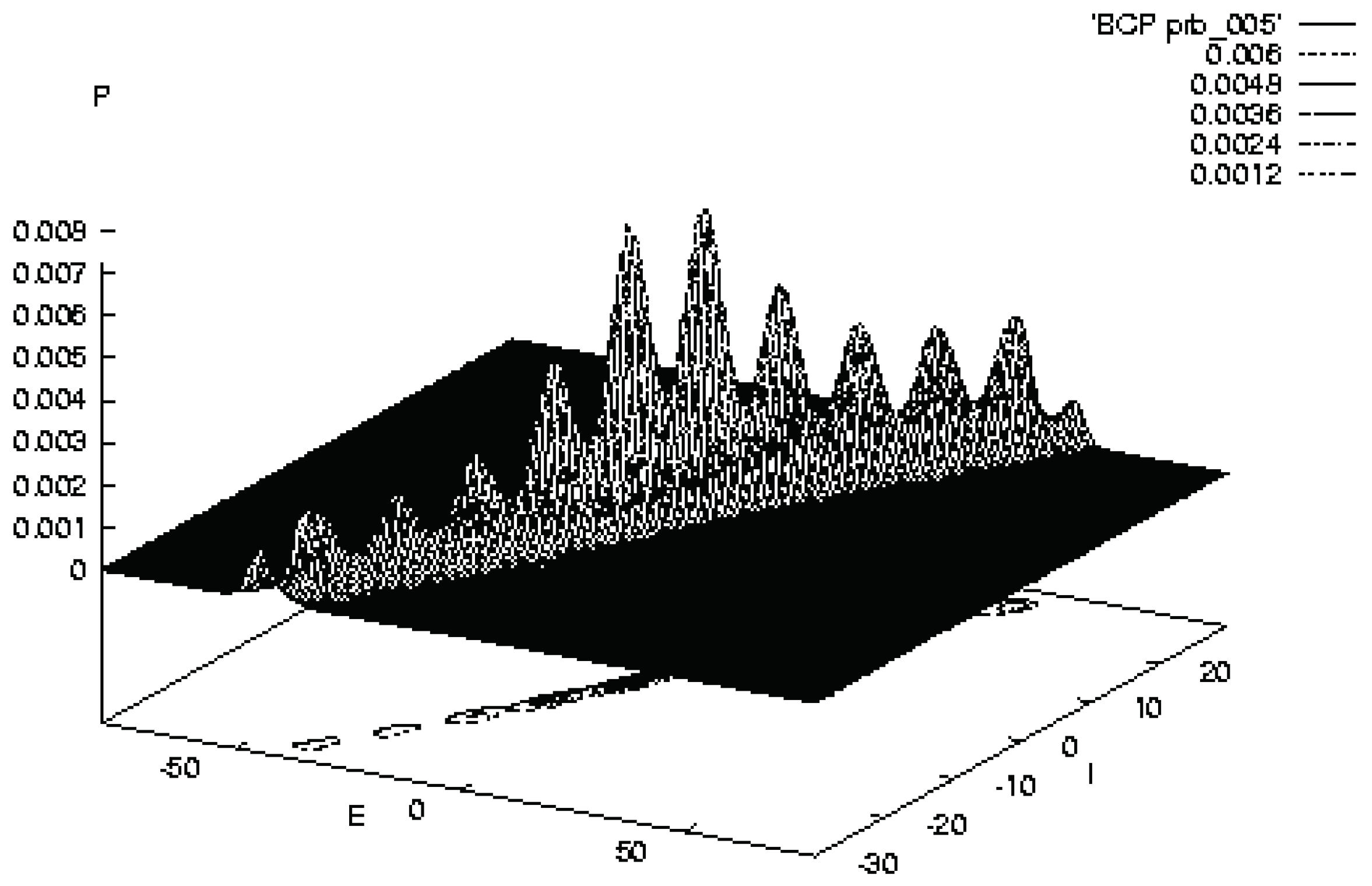
Figure 3.
Illustrates SMNI STM Model BCV at the evolution at 10 [33].
Figure 3.
Illustrates SMNI STM Model BCV at the evolution at 10 [33].

Table 1.
Column 1 is the subject number; the other columns are cost functions. Columns 2 and 3 are no-A model’s Training (TR0) and Testing (TE0). Columns 4 and 5 are A model’s Training (TRA) and Testing (TEA). Columns 6 and 7 are switched no-A model’s Training (sTR0) and Testing (sTE0). Columns 8 and 9 are switched A model’s Training (sTRA) and Testing (sTEA).
| Sub | TR0 | TE0 | TRA | TEA | sTR0 | sTE0 | sTRA | sTEA |
|---|---|---|---|---|---|---|---|---|
| s01 | 85.75 | 121.23 | 84.76 | 121.47 | 120.48 | 86.59 | 119.23 | 87.06 |
| s02 | 70.80 | 51.21 | 68.63 | 56.51 | 51.10 | 70.79 | 49.36 | 74.53 |
| s03 | 61.37 | 79.81 | 59.83 | 78.79 | 79.20 | 61.50 | 75.22 | 79.17 |
| s04 | 52.25 | 64.20 | 50.09 | 66.99 | 63.55 | 52.83 | 63.27 | 64.60 |
| s05 | 67.28 | 72.04 | 66.53 | 72.78 | 71.38 | 67.83 | 69.60 | 68.13 |
| s06 | 84.57 | 69.72 | 80.22 | 64.13 | 69.09 | 84.67 | 61.74 | 114.21 |
| s07 | 68.66 | 78.65 | 68.28 | 86.13 | 78.48 | 68.73 | 75.57 | 69.58 |
| s08 | 46.58 | 43.81 | 44.24 | 49.38 | 43.28 | 47.27 | 42.89 | 63.09 |
| s09 | 47.22 | 24.88 | 46.90 | 25.77 | 24.68 | 47.49 | 24.32 | 49.94 |
| s10 | 53.18 | 33.33 | 53.33 | 36.97 | 33.14 | 53.85 | 30.32 | 55.78 |
| s11 | 43.98 | 51.10 | 43.29 | 52.76 | 50.95 | 44.47 | 50.25 | 45.85 |
| s12 | 45.78 | 45.14 | 44.38 | 46.08 | 44.92 | 46.00 | 44.45 | 46.56 |
© 2019 by the author. Licensee MDPI, Basel, Switzerland. This article is an open access article distributed under the terms and conditions of the Creative Commons Attribution (CC BY) license (http://creativecommons.org/licenses/by/4.0/).
Share and Cite
MDPI and ACS Style
Ingber, L. Quantum Calcium-Ion Interactions with EEG. Sci 2019, 1, 20. https://doi.org/10.3390/sci1010020
AMA Style
Ingber L. Quantum Calcium-Ion Interactions with EEG. Sci. 2019; 1(1):20. https://doi.org/10.3390/sci1010020
Chicago/Turabian StyleIngber, Lester. 2019. "Quantum Calcium-Ion Interactions with EEG" Sci 1, no. 1: 20. https://doi.org/10.3390/sci1010020
APA StyleIngber, L. (2019). Quantum Calcium-Ion Interactions with EEG. Sci, 1(1), 20. https://doi.org/10.3390/sci1010020