

Fractality–Autoencoder-Based Methodology to Detect Corrosion Damage in a Truss-Type Bridge

 ,
,  ,
,  ,
,  and
and 
Abstract
1. Introduction
2. Theoretical Background
2.1. Fractal Dimension
2.1.1. Katz Fractal Dimension
2.1.2. Higuchi Fractal Dimension
2.1.3. Box Counting Fractal Dimension
2.1.4. Petrosian Fractal Dimension
2.1.5. Sevcik Fractal Dimension
2.1.6. Castiglioni Fractal Dimension
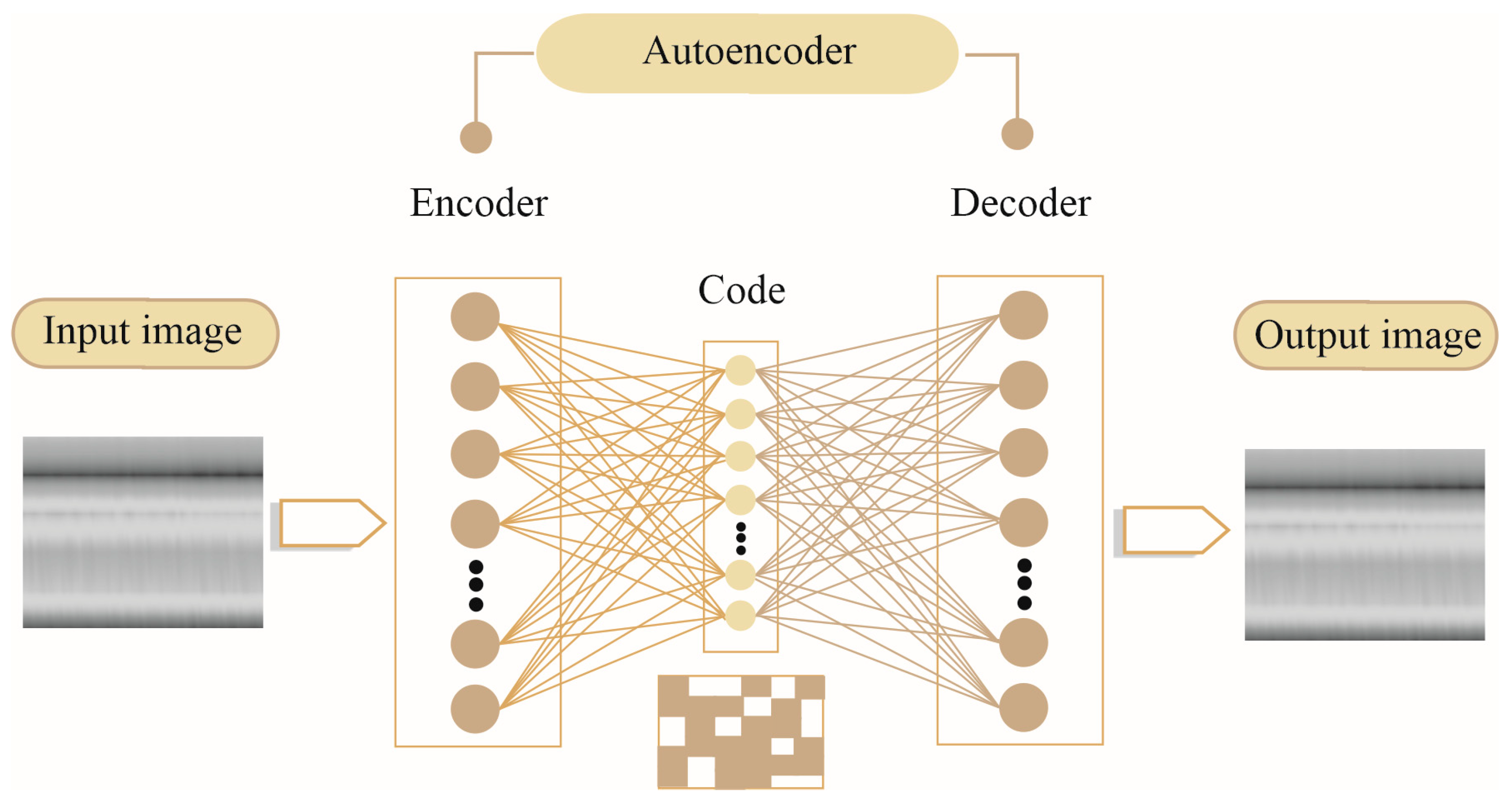
2.2. Autencoder
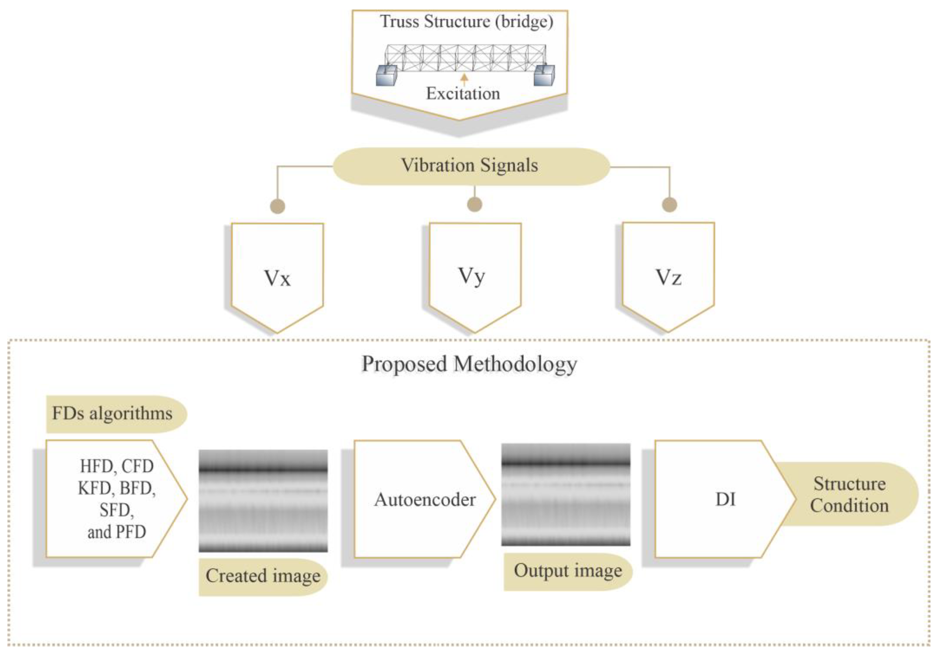
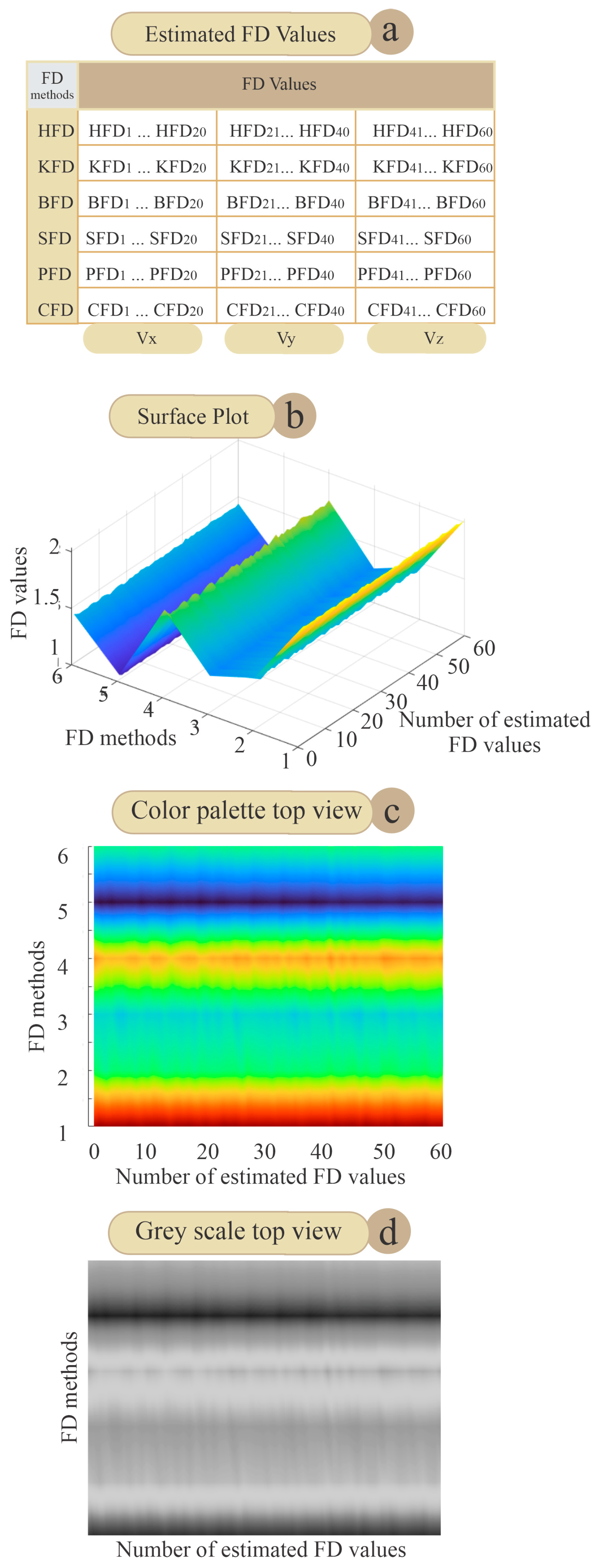
3. Methodology
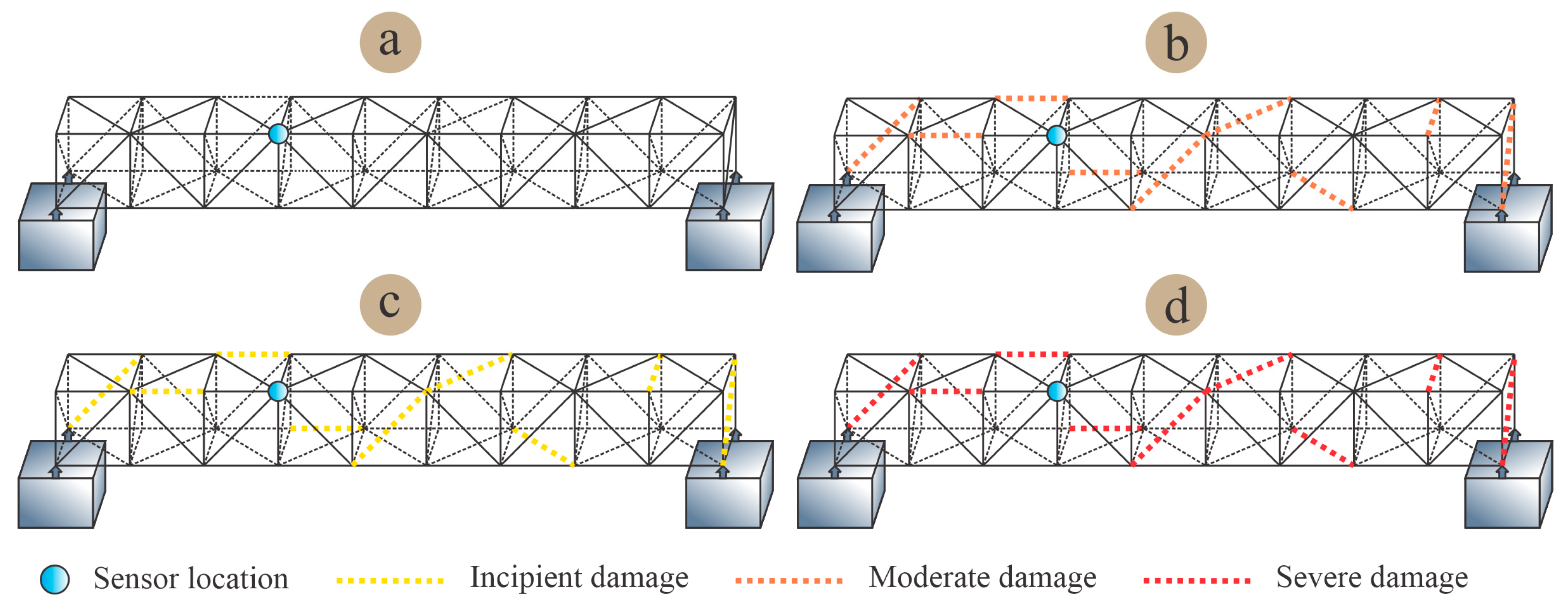
4. Experimental Setup
Damaged Elements
5. Results
6. Discussion
7. Conclusions
Author Contributions
Funding
Institutional Review Board Statement
Informed Consent Statement
Data Availability Statement
Conflicts of Interest
References
- Gonzalez, A.; Schorr, M.; Valdez, B.; Mungaray, A.; Gonzalez, A.; Schorr, M.; Valdez, B.; Mungaray, A. Bridges: Structures and Materials, Ancient and Modern. In Infrastructure Management and Construction; IntechOpen: London, UK, 2020; ISBN 978-1-78984-549-5. [Google Scholar]
- Hao, H.; Bi, K.; Chen, W.; Pham, T.M.; Li, J. Towards next Generation Design of Sustainable, Durable, Multi-Hazard Resistant, Resilient, and Smart Civil Engineering Structures. Eng. Struct. 2023, 277, 115477. [Google Scholar] [CrossRef]
- van de Velde, M.; Vandecruys, E.; Verstrynge, E.; Reynders, E.; Lombaert, G. Vibration Monitoring and Acoustic Emission Sensing during Progressive Load Tests of Corroded Reinforced Concrete Beams. Eng. Struct. 2024, 306, 117851. [Google Scholar] [CrossRef]
- Schofield, M.J. 33—Corrosion. In Plant Engineer’s Reference Book, 2nd ed.; Snow, D.A., Ed.; Butterworth-Heinemann: Oxford, UK, 2002; pp. 33-1–33-25. ISBN 978-0-7506-4452-5. [Google Scholar]
- Kruger, J.; Begum, S. Corrosion of Metals: Overview. In Reference Module in Materials Science and Materials Engineering; Elsevier: Amsterdam, The Netherlands, 2016; ISBN 978-0-12-803581-8. [Google Scholar]
- Ameli, Z.; Nesheli, S.J.; Landis, E.N. Deep Learning-Based Steel Bridge Corrosion Segmentation and Condition Rating Using Mask RCNN and YOLOv8. Infrastructures 2024, 9, 3. [Google Scholar] [CrossRef]
- Amezquita-Sanchez, J.P.; Adeli, H. Signal Processing Techniques for Vibration-Based Health Monitoring of Smart Structures. Arch. Computat. Methods Eng. 2016, 23, 1–15. [Google Scholar] [CrossRef]
- Melchers, R.E. Probabilistic Models for Corrosion in Structural Reliability Assessment—Part 1: Empirical Models. J. Offshore Mech. Arct. Eng. 2003, 125, 264–271. [Google Scholar] [CrossRef]
- Melchers, R.E. Modeling of Marine Immersion Corrosion for Mild and Low-Alloy Steels—Part 1: Phenomenological Model. Corrosion 2003, 59, 319–334. [Google Scholar] [CrossRef]
- Melchers, R.E. The Effect of Corrosion on the Structural Reliability of Steel Offshore Structures. Corros. Sci. 2005, 47, 2391–2410. [Google Scholar] [CrossRef]
- Huras, L.; Zembaty, Z.; Bońkowski, P.A.; Bobra, P. Quantifying Local Stiffness Loss in Beams Using Rotation Rate Sensors. Mech. Syst. Signal Process. 2021, 151, 107396. [Google Scholar] [CrossRef]
- Sokołowski, D.; Kamiński, M. Stochastic Reliability-Based Design Optimization Framework for the Steel Plate Girder with Corrugated Web Subjected to Corrosion. Materials 2022, 15, 7170. [Google Scholar] [CrossRef]
- Melchers, R.E. Corrosion Uncertainty Modelling for Steel Structures. J. Constr. Steel Res. 1999, 52, 3–19. [Google Scholar] [CrossRef]
- Mishra, M.; Lourenço, P.B.; Ramana, G.V. Structural Health Monitoring of Civil Engineering Structures by Using the Internet of Things: A Review. J. Build. Eng. 2022, 48, 103954. [Google Scholar] [CrossRef]
- Agyemang, I.O.; Zhang, X.; Adjei-Mensah, I.; Acheampong, D.; Fiasam, L.D.; Sey, C.; Yussif, S.B.; Effah, D. Automated Vision-Based Structural Health Inspection and Assessment for Post-Construction Civil Infrastructure. Autom. Constr. 2023, 156, 105153. [Google Scholar] [CrossRef]
- Smarsly, K.; Dragos, K.; Stührenberg, J.; Worm, M. Mobile Structural Health Monitoring Based on Legged Robots. Infrastructures 2023, 8, 136. [Google Scholar] [CrossRef]
- Avci, O.; Abdeljaber, O.; Kiranyaz, S.; Hussein, M.; Gabbouj, M.; Inman, D.J. A Review of Vibration-Based Damage Detection in Civil Structures: From Traditional Methods to Machine Learning and Deep Learning Applications. Mech. Syst. Signal Process. 2021, 147, 107077. [Google Scholar] [CrossRef]
- Hasani, H.; Freddi, F. Operational Modal Analysis on Bridges: A Comprehensive Review. Infrastructures 2023, 8, 172. [Google Scholar] [CrossRef]
- Amezquita-Sanchez, J.P. Entropy Algorithms for Detecting Incipient Damage in High-Rise Buildings Subjected to Dynamic Vibrations. J. Vib. Control. 2021, 27, 426–436. [Google Scholar] [CrossRef]
- Deng, Z.; Huang, M.; Wan, N.; Zhang, J. The Current Development of Structural Health Monitoring for Bridges: A Review. Buildings 2023, 13, 1360. [Google Scholar] [CrossRef]
- Luo, J.; Zheng, F.; Sun, S. A Few-Shot Learning Method for Vibration-Based Damage Detection in Civil Structures. Structures 2024, 61, 106026. [Google Scholar] [CrossRef]
- Poorghasem, S.; Bao, Y. Review of Robot-Based Automated Measurement of Vibration for Civil Engineering Structures. Measurement 2023, 207, 112382. [Google Scholar] [CrossRef]
- Hou, R.; Xia, Y. Review on the New Development of Vibration-Based Damage Identification for Civil Engineering Structures: 2010–2019. J. Sound Vib. 2021, 491, 115741. [Google Scholar] [CrossRef]
- Yu, X.; Fu, Y.; Li, J.; Mao, J.; Hoang, T.; Wang, H. Recent Advances in Wireless Sensor Networks for Structural Health Monitoring of Civil Infrastructure. J. Infrastruct. Intell. Resil. 2024, 3, 100066. [Google Scholar] [CrossRef]
- Avci, O.; Abdeljaber, O.; Kiranyaz, S.; Hussein, M.; Inman, D.J. Wireless and Real-Time Structural Damage Detection: A Novel Decentralized Method for Wireless Sensor Networks. J. Sound Vib. 2018, 424, 158–172. [Google Scholar] [CrossRef]
- Amezquita-Sanchez, J.P.; Adeli, H. Nonlinear Measurements for Feature Extraction in Structural Health Monitoring. Sci. Iran. 2019, 26, 3051–3059. [Google Scholar] [CrossRef]
- Vafaei, M.; Alih, S.C. Adequacy of First Mode Shape Differences for Damage Identification of Cantilever Structures Using Neural Networks. Neural Comput. Appl. 2018, 30, 2509–2518. [Google Scholar] [CrossRef]
- Datteo, A.; Lucà, F.; Busca, G. Statistical Pattern Recognition Approach for Long-Time Monitoring of the G.Meazza Stadium by Means of AR Models and PCA. Eng. Struct. 2017, 153, 317–333. [Google Scholar] [CrossRef]
- Datteo, A.; Busca, G.; Quattromani, G.; Cigada, A. On the Use of AR Models for SHM: A Global Sensitivity and Uncertainty Analysis Framework. Reliab. Eng. Syst. Saf. 2018, 170, 99–115. [Google Scholar] [CrossRef]
- Shi, B.; Qiao, P. A New Surface Fractal Dimension for Displacement Mode Shape-Based Damage Identification of Plate-Type Structures. Mech. Syst. Signal Process. 2018, 103, 139–161. [Google Scholar] [CrossRef]
- Li, H.; Bao, Y.; Ou, J. Structural Damage Identification Based on Integration of Information Fusion and Shannon Entropy. Mech. Syst. Signal Process. 2008, 22, 1427–1440. [Google Scholar] [CrossRef]
- Kankanamge, Y.; Hu, Y.; Shao, X. Application of Wavelet Transform in Structural Health Monitoring. Earthq. Eng. Eng. Vib. 2020, 19, 515–532. [Google Scholar] [CrossRef]
- Azami, M.; Salehi, M. Response-Based Multiple Structural Damage Localization through Multi-Channel Empirical Mode Decomposition. J. Struct. Integr. Maint. 2019, 4, 195–206. [Google Scholar] [CrossRef]
- Jiang, X.; Adeli, H. Pseudospectra, MUSIC, and Dynamic Wavelet Neural Network for Damage Detection of Highrise Buildings. Int. J. Numer. Methods Eng. 2007, 71, 606–629. [Google Scholar] [CrossRef]
- Tibaduiza, D.; Torres-Arredondo, M.Á.; Vitola, J.; Anaya, M.; Pozo, F. A Damage Classification Approach for Structural Health Monitoring Using Machine Learning. Complexity 2018, 2018, 5081283. [Google Scholar] [CrossRef]
- Rabcan, J.; Levashenko, V.; Zaitseva, E.; Kvassay, M.; Subbotin, S. Non-Destructive Diagnostic of Aircraft Engine Blades by Fuzzy Decision Tree. Eng. Struct. 2019, 197, 109396. [Google Scholar] [CrossRef]
- Padil, K.H.; Bakhary, N.; Abdulkareem, M.; Li, J.; Hao, H. Non-Probabilistic Method to Consider Uncertainties in Frequency Response Function for Vibration-Based Damage Detection Using Artificial Neural Network. J. Sound Vib. 2020, 467, 115069. [Google Scholar] [CrossRef]
- Lin, T.-K.; Chen, Y.-C. Integration of Refined Composite Multiscale Cross-Sample Entropy and Backpropagation Neural Networks for Structural Health Monitoring. Appl. Sci. 2020, 10, 839. [Google Scholar] [CrossRef]
- Ruocci, G.; Cumunel, G.; Le, T.; Argoul, P.; Point, N.; Dieng, L. Damage Assessment of Pre-Stressed Structures: A SVD-Based Approach to Deal with Time-Varying Loading. Mech. Syst. Signal Process. 2014, 47, 50–65. [Google Scholar] [CrossRef]
- Abu-Mahfouz, I.; Banerjee, A. Crack Detection and Identification Using Vibration Signals and Fuzzy Clustering. Procedia Comput. Sci. 2017, 114, 266–274. [Google Scholar] [CrossRef]
- Valtierra-Rodriguez, M.; Rivera-Guillen, J.R.; Basurto-Hurtado, J.A.; De-Santiago-Perez, J.J.; Granados-Lieberman, D.; Amezquita-Sanchez, J.P. Convolutional Neural Network and Motor Current Signature Analysis during the Transient State for Detection of Broken Rotor Bars in Induction Motors. Sensors 2020, 20, 3721. [Google Scholar] [CrossRef]
- Cha, Y.-J.; Ali, R.; Lewis, J.; Büyüköztürk, O. Deep Learning-Based Structural Health Monitoring. Autom. Constr. 2024, 161, 105328. [Google Scholar] [CrossRef]
- Eltouny, K.; Gomaa, M.; Liang, X. Unsupervised Learning Methods for Data-Driven Vibration-Based Structural Health Monitoring: A Review. Sensors 2023, 23, 3290. [Google Scholar] [CrossRef]
- Ghazimoghadam, S.; Hosseinzadeh, S.A.A. A Novel Unsupervised Deep Learning Approach for Vibration-Based Damage Diagnosis Using a Multi-Head Self-Attention LSTM Autoencoder. Measurement 2024, 229, 114410. [Google Scholar] [CrossRef]
- Sarwar, M.Z.; Cantero, D. Probabilistic Autoencoder-Based Bridge Damage Assessment Using Train-Induced Responses. Mech. Syst. Signal Process. 2024, 208, 111046. [Google Scholar] [CrossRef]
- Giglioni, V.; Venanzi, I.; Poggioni, V.; Milani, A.; Ubertini, F. Autoencoders for Unsupervised Real-Time Bridge Health Assessment. Comput.-Aided Civ. Infrastruct. Eng. 2023, 38, 959–974. [Google Scholar] [CrossRef]
- Coraça, E.M.; Ferreira, J.V.; Nóbrega, E.G.O. An Unsupervised Structural Health Monitoring Framework Based on Variational Autoencoders and Hidden Markov Models. Reliab. Eng. Syst. Saf. 2023, 231, 109025. [Google Scholar] [CrossRef]
- Junges, R.; Rastin, Z.; Lomazzi, L.; Giglio, M.; Cadini, F. Convolutional Autoencoders and CGANs for Unsupervised Structural Damage Localization. Mech. Syst. Signal Process. 2024, 220, 111645. [Google Scholar] [CrossRef]
- Li, P.; Pei, Y.; Li, J. A Comprehensive Survey on Design and Application of Autoencoder in Deep Learning. Appl. Soft Comput. 2023, 138, 110176. [Google Scholar] [CrossRef]
- Hoxha, E.; Vidal, Y.; Pozo, F. Damage Diagnosis for Offshore Wind Turbine Foundations Based on the Fractal Dimension. Appl. Sci. 2020, 10, 6972. [Google Scholar] [CrossRef]
- Bao, Y.; Li, H. Machine Learning Paradigm for Structural Health Monitoring. Struct. Health Monit. 2021, 20, 1353–1372. [Google Scholar] [CrossRef]
- Xu, N.; Zhang, Z.; Liu, Y. 14—Spatiotemporal Fractal Manifold Learning for Vibration-Based Structural Health Monitoring. In Structural Health Monitoring/Management (SHM) in Aerospace Structures; Yuan, F.-G., Ed.; Woodhead Publishing Series in Composites Science and Engineering; Woodhead Publishing: Sawston, UK, 2024; pp. 409–426. ISBN 978-0-443-15476-8. [Google Scholar]
- Katz, M.J. Fractals and the Analysis of Waveforms. Comput. Biol. Med. 1988, 18, 145–156. [Google Scholar] [CrossRef]
- Higuchi, T. Approach to an Irregular Time Series on the Basis of the Fractal Theory. Phys. D Nonlinear Phenom. 1988, 31, 277–283. [Google Scholar] [CrossRef]
- Petrosian, A. Kolmogorov Complexity of Finite Sequences and Recognition of Different Preictal EEG Patterns. In Proceedings of the Proceedings Eighth IEEE Symposium on Computer-Based Medical Systems, Lubbock, TX, USA, 9–10 June 1995; pp. 212–217. [Google Scholar]
- Sevcik, C. A Procedure to Estimate the Fractal Dimension of Waveforms. Complex Int. 1998, 5, 1–19. Available online: https://arxiv.org/pdf/1003.5266 (accessed on 23 July 2024).
- Wang, B. Detection of Structural Damage Using Fractal Dimension Technique. Zhendong Yu Chongji (J. Vibr. Shock) 2005, 24, 87–88. [Google Scholar]
- Castiglioni, P. What Is Wrong in Katz’s Method? Comments on: “A Note on Fractal Dimensions of Biomedical Waveforms”. Comput. Biol. Med. 2010, 40, 950–952. [Google Scholar] [CrossRef]
- Medina, R.; Sánchez, R.-V.; Cabrera, D.; Cerrada, M.; Estupiñan, E.; Ao, W.; Vásquez, R.E. Scale-Fractal Detrended Fluctuation Analysis for Fault Diagnosis of a Centrifugal Pump and a Reciprocating Compressor. Sensors 2024, 24, 461. [Google Scholar] [CrossRef] [PubMed]
- Captur, G.; Karperien, A.L.; Hughes, A.D.; Francis, D.P.; Moon, J.C. The Fractal Heart—Embracing Mathematics in the Cardiology Clinic. Nat. Rev. Cardiol. 2017, 14, 56–64. [Google Scholar] [CrossRef] [PubMed]
- Du, B.; Xiong, W.; Wu, J.; Zhang, L.; Zhang, L.; Tao, D. Stacked Convolutional Denoising Auto-Encoders for Feature Representation. IEEE Trans. Cybern. 2017, 47, 1017–1027. [Google Scholar] [CrossRef] [PubMed]
- Liu, P.; Zheng, P.; Chen, Z. Deep Learning with Stacked Denoising Auto-Encoder for Short-Term Electric Load Forecasting. Energies 2019, 12, 2445. [Google Scholar] [CrossRef]
- Agarwala, A.; Pennington, J.; Dauphin, Y.; Schoenholz, S. Temperature Check: Theory and Practice for Training Models with Softmax-Cross-Entropy Losses. arXiv 2020, arXiv:2010.07344. [Google Scholar]
- Tabiatnejad, D.; Tabiatnejad, B.; Khedmatgozar Dolati, S.S.; Mehrabi, A. Damage Detection in External Tendons of Post-Tensioned Bridges. Infrastructures 2024, 9, 103. [Google Scholar] [CrossRef]
- Moghadam, A.; Melhem, H.G.; Esmaeily, A. A Proof-of-Concept Study on a Proposed Ambient-Vibration-Based Approach to Extract Pseudo-Free-Vibration Response. Eng. Struct. 2020, 212, 110517. [Google Scholar] [CrossRef]
- Abdeljaber, O.; Avci, O.; Kiranyaz, S.; Gabbouj, M.; Inman, D.J. Real-Time Vibration-Based Structural Damage Detection Using One-Dimensional Convolutional Neural Networks. J. Sound Vib. 2017, 388, 154–170. [Google Scholar] [CrossRef]
- Hagara, M.; Stojanović, R.; Bagala, T.; Kubinec, P.; Ondráček, O. Grayscale Image Formats for Edge Detection and for Its FPGA Implementation. Microprocess. Microsyst. 2020, 75, 103056. [Google Scholar] [CrossRef]
- Blachowski, B.; An, Y.; Spencer, B.F., Jr.; Ou, J. Axial Strain Accelerations Approach for Damage Localization in Statically Determinate Truss Structures. Comput.-Aided Civ. Infrastruct. Eng. 2017, 32, 304–318. [Google Scholar] [CrossRef]
- Khodabandehlou, H.; Pekcan, G.; Fadali, M.S. Vibration-Based Structural Condition Assessment Using Convolution Neural Networks. Struct. Control. Health Monit. 2019, 26, e2308. [Google Scholar] [CrossRef]
- Rafiei, M.H.; Adeli, H. A Novel Machine Learning-based Algorithm to Detect Damage in High-rise Building Structures. Struct. Des. Tall Spec. Build. 2017, 26, e1400. Available online: https://onlinelibrary.wiley.com/doi/abs/10.1002/tal.1400 (accessed on 23 July 2024). [CrossRef]
- Sydenham, P.H. Chapter 11—Vibration. In Instrumentation Reference Book, 4th ed.; Boyes, W., Ed.; Butterworth-Heinemann: Boston, MA, USA, 2010; pp. 113–125. ISBN 978-0-7506-8308-1. [Google Scholar]
- Lin, J.-F.; Xu, Y.-L.; Law, S.-S. Structural Damage Detection-Oriented Multi-Type Sensor Placement with Multi-Objective Optimization. J. Sound Vib. 2018, 422, 568–589. [Google Scholar] [CrossRef]
- Affonso, L.O.A. 7—Corrosion. In Machinery Failure Analysis Handbook; Affonso, L.O.A., Ed.; Gulf Publishing Company: Houston, TX, USA, 2006; pp. 83–99. ISBN 978-1-933762-08-1. [Google Scholar]
- Liu, D.; Qiu, X.; Shao, M.; Gao, J.; Xu, J.; Liu, Q.; Zhou, H.; Wang, Z. Synthesis and Evaluation of Hexamethylenetetramine Quaternary Ammonium Salt as Corrosion Inhibitor. Mater. Corros. 2019, 70, 1907–1916. [Google Scholar] [CrossRef]
- Pang, B.; Qian, J.; Zhang, Y.; Jia, Y.; Ni, H.; Pang, S.D.; Liu, G.; Qian, R.; She, W.; Yang, L.; et al. 5S Multifunctional Intelligent Coating with Superdurable, Superhydrophobic, Self-Monitoring, Self-Heating, and Self-Healing Properties for Existing Construction Application. ACS Appl. Mater. Interfaces 2019, 11, 29242–29254. [Google Scholar] [CrossRef]
- Park, S.; Park, S.-K. Quantitative Corrosion Monitoring Using Wireless Electromechanical Impedance Measurements. Res. Nondestruct. Eval. 2010, 21, 184–192. [Google Scholar] [CrossRef]
- Moreno-Gomez, A.; Amezquita-Sanchez, J.P.; Valtierra-Rodriguez, M.; Perez-Ramirez, C.A.; Dominguez-Gonzalez, A.; Chavez-Alegria, O. EMD-Shannon Entropy-Based Methodology to Detect Incipient Damages in a Truss Structure. Appl. Sci. 2018, 8, 2068. [Google Scholar] [CrossRef]
- Marcot, B.G.; Hanea, A.M. What Is an Optimal Value of k in K-Fold Cross-Validation in Discrete Bayesian Network Analysis? Comput. Stat. 2021, 36, 2009–2031. [Google Scholar] [CrossRef]
- Yang, L.; Fu, C.; Li, Y.; Su, L. Survey and Study on Intelligent Monitoring and Health Management for Large Civil Structure. Int. J. Intell. Robot. Appl. 2019, 3, 239–254. [Google Scholar] [CrossRef]
- Babajanian Bisheh, H.; Ghodrati Amiri, G.; Nekooei, M.; Darvishan, E. Damage Detection of a Cable-Stayed Bridge Using Feature Extraction and Selection Methods. Struct. Infrastruct. Eng. 2019, 15, 1165–1177. [Google Scholar] [CrossRef]
- Yang, J.; Li, P.; Yang, Y.; Xu, D. An Improved EMD Method for Modal Identification and a Combined Static-Dynamic Method for Damage Detection. J. Sound Vib. 2018, 420, 242–260. [Google Scholar] [CrossRef]
- Chen, Z.; Pan, C.; Yu, L. Structural Damage Detection via Adaptive Dictionary Learning and Sparse Representation of Measured Acceleration Responses. Measurement 2018, 128, 377–387. [Google Scholar] [CrossRef]
- Zamani HosseinAbadi, H.; Amirfattahi, R.; Nazari, B.; Mirdamadi, H.R.; Atashipour, S.A. GUW-Based Structural Damage Detection Using WPT Statistical Features and Multiclass SVM. Appl. Acoust. 2014, 86, 59–70. [Google Scholar] [CrossRef]


| No. Neurons | Loss Value | Estimated Error |
|---|---|---|
| 100 | 1.8456 × 10⁻⁴ | 1.7902 × 10⁻⁴ |
| 90 | 2.3020 × 10⁻⁴ | 1.9357 × 10⁻⁴ |
| 80 | 3.9727 × 10⁻⁴ | 3.2216 × 10⁻⁴ |
| 70 | 4.2435 × 10⁻⁴ | 4.0953 × 10⁻⁴ |
| 60 | 2.2616 × 10⁻⁴ | 2.1101 × 10⁻⁴ |
| 50 | 2.6931 × 10⁻⁴ | 2.5435 × 10⁻⁴ |
| 40 | 2.6117 × 10⁻⁴ | 2.3685 × 10⁻⁴ |
| 30 | 1.6913 × 10⁻⁴ | 1.5919 × 10⁻⁴ |
| 20 | 2.2099 × 10⁻⁴ | 2.0457 × 10⁻⁴ |
| 10 | 2.4064 × 10⁻⁴ | 2.0065 × 10⁻⁴ |
| Truss Structure Condition | Predicted | Effectiveness (%) | ||
|---|---|---|---|---|
| Healthy | Corrosion | |||
| Actual | Healthy | 30 | 0 | 100 |
| Corrosion | 10 | 2690 | 99.6 | |
| Total accuracy (%) | 99.8 | |||
Disclaimer/Publisher’s Note: The statements, opinions and data contained in all publications are solely those of the individual author(s) and contributor(s) and not of MDPI and/or the editor(s). MDPI and/or the editor(s) disclaim responsibility for any injury to people or property resulting from any ideas, methods, instructions or products referred to in the content. |
© 2024 by the authors. Licensee MDPI, Basel, Switzerland. This article is an open access article distributed under the terms and conditions of the Creative Commons Attribution (CC BY) license (https://creativecommons.org/licenses/by/4.0/).
Share and Cite
Valtierra-Rodriguez, M.; Machorro-Lopez, J.M.; Yanez-Borjas, J.J.; Perez-Quiroz, J.T.; Rivera-Guillen, J.R.; Amezquita-Sanchez, J.P. Fractality–Autoencoder-Based Methodology to Detect Corrosion Damage in a Truss-Type Bridge. Infrastructures 2024, 9, 145. https://doi.org/10.3390/infrastructures9090145
Valtierra-Rodriguez M, Machorro-Lopez JM, Yanez-Borjas JJ, Perez-Quiroz JT, Rivera-Guillen JR, Amezquita-Sanchez JP. Fractality–Autoencoder-Based Methodology to Detect Corrosion Damage in a Truss-Type Bridge. Infrastructures. 2024; 9(9):145. https://doi.org/10.3390/infrastructures9090145
Chicago/Turabian StyleValtierra-Rodriguez, Martin, Jose M. Machorro-Lopez, Jesus J. Yanez-Borjas, Jose T. Perez-Quiroz, Jesus R. Rivera-Guillen, and Juan P. Amezquita-Sanchez. 2024. "Fractality–Autoencoder-Based Methodology to Detect Corrosion Damage in a Truss-Type Bridge" Infrastructures 9, no. 9: 145. https://doi.org/10.3390/infrastructures9090145
APA StyleValtierra-Rodriguez, M., Machorro-Lopez, J. M., Yanez-Borjas, J. J., Perez-Quiroz, J. T., Rivera-Guillen, J. R., & Amezquita-Sanchez, J. P. (2024). Fractality–Autoencoder-Based Methodology to Detect Corrosion Damage in a Truss-Type Bridge. Infrastructures, 9(9), 145. https://doi.org/10.3390/infrastructures9090145