Article

Analyzing Wind Effects on Long-Span Bridges: A Viable Numerical Modelling Methodology Using OpenFOAM for Industrial Applications

1
B-Fluid, D02 FK19 Dublin, Ireland
2
Arup, D04 T6X0 Dublin, Ireland
3
School of Mechanical and Materials Engineering, University College Dublin, D04 V1W8 Dublin, Ireland
4
School of Civil Engineering, University College Dublin, D04 V1W8 Dublin, Ireland
*
Author to whom correspondence should be addressed.
Infrastructures 2023, 8(9), 130; https://doi.org/10.3390/infrastructures8090130
Submission received: 12 May 2023 / Revised: 21 August 2023 / Accepted: 23 August 2023 / Published: 26 August 2023
(This article belongs to the Special Issue Bridge Modeling, Monitoring, Management and Beyond)

Abstract

:
Aerodynamic performance is of critical importance to the design of long-span bridges. Computational fluid dynamics (CFD) modelling offers bridge designers an opportunity to investigate aerodynamic performance for long-span bridges during the design phase as well as during operation of the bridge. It offers distinct advantages when compared with the current standard practice of wind tunnel testing, which can have several limitations. The proposed revisions to the Eurocodes offer CFD as a methodology for wind analysis of bridges. Practicing engineers have long sought a computationally affordable, viable, and robust framework for industrial applications of using CFD to examine wind effects on long-span bridges. To address this gap in the literature and guidance, this paper explicitly presents a framework and demonstrates a workflow of analyzing wind effects on long-span bridges using open-source software, namely FreeCAD, OpenFOAM, and ParaView. Example cases are presented, and detailed configurations and general guidance are discussed during each step. A summary is provided of the validation of this methodology with field data collected from the structural health monitoring (SHM) systems of two long-span bridges.

1. Introduction

Assessment of the wind effects on long-span bridges is a critical aspect of their safe design. When wind blows on a bridge, it exerts a distributed pressure force on the structure, which is related to the velocity of the wind. Forces are resisted by bridges and transferred to the ground through mechanisms of bending, torsion, and shear. In exposed sites, wind loads can sometimes have a greater impact than any other bridge load, such as thermal loading and traffic loading [1]. An essential role of any bridge engineer is to estimate the effects of prevailing wind conditions on a bridge and suitably design the various bridge elements for this loading, yet the forces that bridges experience in high winds are poorly understood. More specifically, when designing long-span bridges, engineers can face aerodynamic and aeroelastic challenges due to wind effects, such as buffeting [2], flutter [3], vortex-induced vibrations [4], galloping [5], and cable vibrations [6]. To predict and estimate the influences of these problems on bridge design, several key parameters are of interest, namely the aerodynamic coefficients, vortex shedding frequencies, and flutter derivatives. The aerodynamic coefficients are typically the most frequently used. They are dimensionless coefficients that are used in calculations of aerodynamic forces and flutter derivatives.
The accepted state of the art is that bridge design is based on wind tunnel testing [7,8,9,10]. Although wind tunnel testing for design offers data, the data are limited due to assumptions of stationarity and scalability, particularly of Reynolds and Strouhal numbers. Furthermore, locations of sensors must be decided a priori and can only provide information at discrete measurement points. Flow visualization of the entire domain (e.g., PIV) is typically prohibitively complicated and expensive. Scheduling time at a wind tunnel facility can prove expensive both in terms of time and cost, particularly when repeat tests might need to be conducted. Aerodynamic admittance, based on the seminal work of both Davenport and Scanlan, is assumed to act strip wise (1D) for bridges to create the buffeting forces, and only recently have new analytical forms been proposed [11] to reflect the growing length and complexity of bridges. This increasingly means that 1D and zero-yaw angle winds are no longer reasonable assumptions, and together with the previous limitations, this makes wind tunnel testing hugely limiting for this application.
The opportunities afforded by the advent of greater computational capacity offers the use of computational fluid dynamics (CFD) as an alternative method [12,13,14,15,16,17]. Even in the early stages of development, when computational power was significantly limited, some pioneers [18,19,20,21,22,23] demonstrated the capacity of CFD simulations in this area. CFD has been used to assess the non-uniform wind characteristics in mountainous areas and its effects on the flutter performance of a long-span suspension bridge [24]. In July 2008, a benchmark study on the aerodynamics of rectangular cylinders was initiated with the aim of analyzing the turbulence and separated flow around an elongated rectangular cylinder, analogous to a bridge [25,26,27,28,29,30]. Analyses have used both CFD and WTT, and results have yielded valuable insights. Computational methods have been used to investigate the edge degree-of-sharpness and free-stream turbulence scale effects on the aerodynamics of a bridge deck [31] to investigate the impact of gap distance between twin-box decks [32], as well as to optimize the shape of bridge decks considering aeroelastic and structural constraints [33,34]. More recently, authors have begun to investigate the effects of bridge deck movement as part of these computational analyses [35,36,37,38].
Currently, the Eurocode on wind actions [39] provides guidance on calculating wind effects under specific conditions with sets of equations and recommends wind tunnel testing in all other conditions. CFD is not yet specified in the Eurocode as a means of estimating wind effects on long-span bridges. Interestingly, the Eurocodes are currently undergoing revision, and the latest draft includes an annex permitting the use of CFD in certain circumstances [40]. However, there is a lack of prescriptive guidance to accompany these design codes for bridge design engineers. There is demand from bridge designers, bridge owners, and bridge operators for a CFD methodology that they can use in assessing their existing bridge stock for adverse impacts due to prevailing wind conditions, as well as assessing newly planned bridges [41]. According to Zhang et al. [42], many publications that present analysis of wind effects on bridges using CFD have provided descriptions of their methodology in relatively little detail and rather choose to focus on analyses of the results [43,44,45]. Most currently available online guidance does not consider the unique application of wind effects on long-span bridges. The National Standards Authority of Ireland is currently leading the Irish participation in revisions to the Eurocode on Wind, and therefore this paper directly supports that work. It explicitly articulates an approach to CFD model development that is sufficiently generic as to accommodate many different forms of long-span bridges and that is viable for industrial applications, with enough detail for bridge designers to use in studying wind effects on a sample long-span bridge using OpenFOAM. Crucially, this methodology has been tested and validated with structural health monitoring (SHM) data collected from two long-span bridges in the author’s previous work on the Queensferry Crossing in Edinburgh [22,23] and the Rose Fitzgerald Kennedy Bridge in Ireland [21,46]—further details provided in Section 11. While more sophisticated and more computationally demanding modelling (such as a large eddy simulation incorporating fluid structure interaction) might yield more accurate results, this methodology has been demonstrated to be sufficiently accurate when compared to field data, with a level of computational capacity that makes it viable in industrial applications.
The workflow presented in this paper starts with defining some modelling assumptions in Section 2 followed by developing the geometry, as described in Section 3. After sketching and exporting the 3D geometries to STL files, the configuration of an OpenFOAM case is initiated by creating the computational domain and the mesh (described in Section 4). Next, in Section 5, boundary conditions are specified for different patches. The paper then presents the configurations for multiple dictionaries related to discretization (Section 6), the algorithm solvers (Section 7), and parallel decomposition (Section 8). The process of conducting a mesh sensitivity study is then presented in Section 9. Finally, Section 10 describes the post-processing steps where both quantitative and visualized results are considered. Figure 1 provides an overview of the workflow proposed in this paper.

2. Modelling Assumptions

In an analysis of a typical bridge, the wind velocity at the site will normally have a Mach number that is much smaller than 0.3, and so an assumption of incompressible flow is valid for CFD analysis [47]. Furthermore, the temperature and gravity effects in bridge aerodynamic studies are often neglected, as their contribution to the forces are negligible. During bridge design, aerodynamic coefficients are often used to estimate the aerodynamic performance of a bridge [48,49,50]. These parameters can be calculated from simulations using the Reynolds-averaged Navier–Stokes (RANS) formulations (for example, as implemented in simpleFoam):
∇ · U = 0,
∂U/∂t + ∇ ⋅ (UU) = ∇ ⋅ [νeff (∇U + (∇U)T)] − ∇p
where U is the Reynolds-averaged velocity, p is the Reynolds-averaged kinematic pressure (pressure divided by density), and νeff is the effective kinematic viscosity, which is the summation of laminar kinematic viscosity (ν) and the turbulent kinematic viscosity (νt). The value of the laminar kinematic viscosity, ν, can be configured in the transportProperties file in the constant/directory, which is related to the temperature of the flow. For instance, ν has a value of 1.47 × 10⁻⁵ m2/s at a temperature of 15 °C. In Equation (2), the ∂U/∂t term accounts for transience in the system (URANS) but is omitted for steady-state RANS simulations.
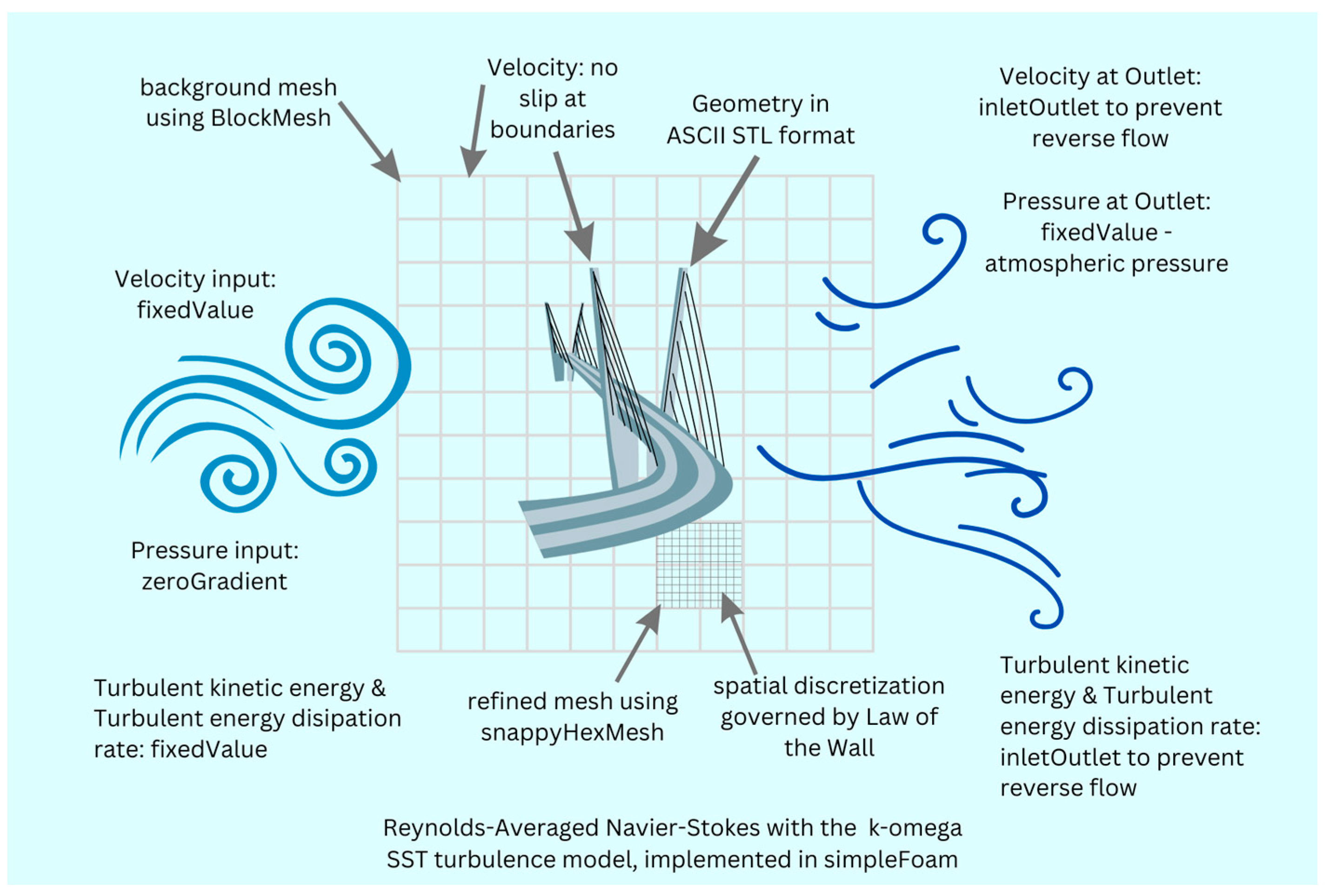
The unknown νt in RANS and URANS simulations can be calculated using various turbulence models. The use of the k-ω SST turbulence model [51] has become popular in the study of bridge aerodynamics [52,53,54] due to its ability to model turbulence behavior in the boundary layer [55]. It should be noted that there are more complex models that might deliver more accurate results, such as the four-equation  v 2 ¯ -f model [56], the four-equation γ-Reθ model [57], and the seven-equation SSG/LRR-ω full Reynolds stress model [58]. Since these models contain more transport equations than the two-equation k-ω SST model, they often require significantly more computational power and are more challenging to converge. Furthermore, the implementation of some of these models, such as the γ-Reθ, also needs empirical correlations to configure inlet parameters, which requires greater effort in calibrating the model to fit specific engineering problems. Given that the purpose of the workflow in this paper is for the engineering design of long-span bridges, computational affordability is of significant importance. In this application, the k-ω SST turbulence model is both affordable and reliable and hence has been proposed for the application of modelling wind effects on bridges in RANS and URANS simulations. To solve the aforementioned governing equations with the k-ω SST turbulence model in OpenFOAM, the simpleFoam solver should be used for RANS simulations, and the pimpleFoam or pisoFoam solver should be used for URANS simulations. In the example case of URANS simulations, the pimpleFoam solver is used because it allows for large time steps, which potentially speeds up the transient simulations. It should be noted that if accurate predictions of turbulence structures are of interest, large-eddy simulations (LESs) [59] and detached-eddy simulations (DESs) [60] are recommended. These simulations can also be performed using the pimpleFoam or pisoFoam solver. However, compared to URANS, LESs and DESs require significantly more computational power. Figure 2 visually depicts key elements of the framework, including boundary conditions, the turbulence model, and discretization methods.

3. Geometry Development

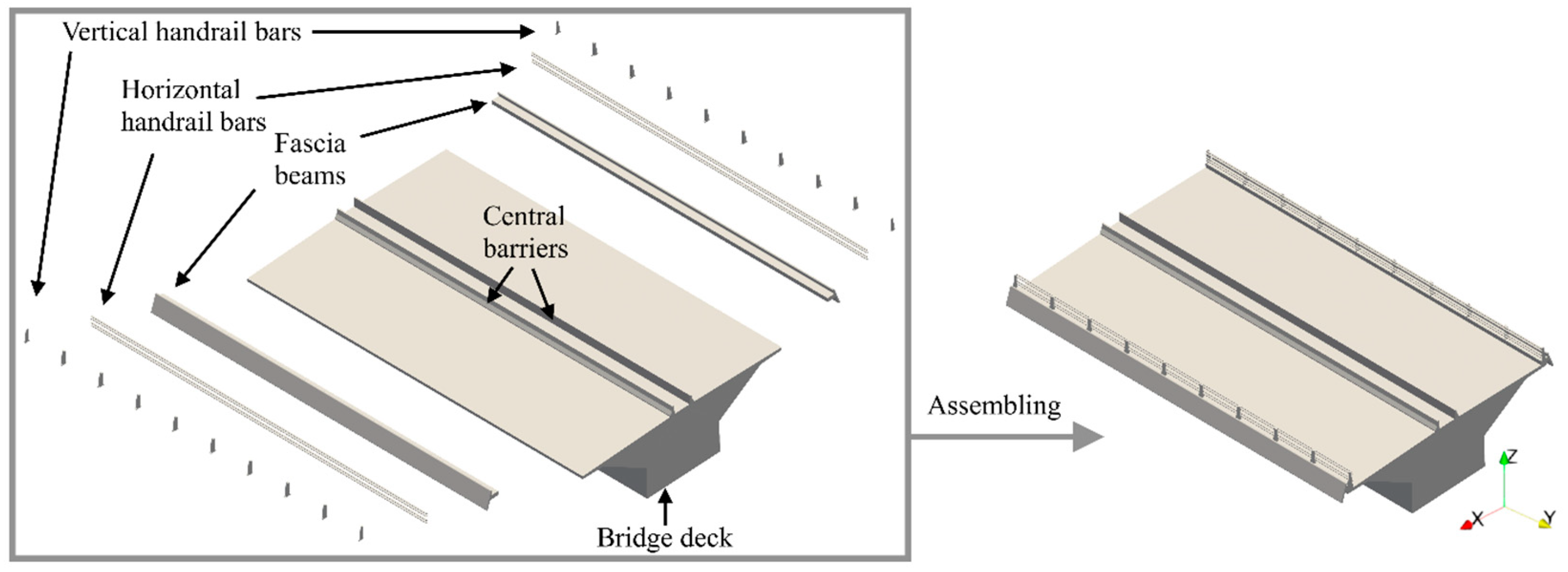
A geometry file describing the bridge structure is a required input of OpenFOAM. There are several software options that can generate 3D bridge geometries. One option is to generate 3D geometries based on 2D sketches using AutoCAD version 2021, commonly used software in civil engineering designs. Based on the authors’ experience, 3D solids sketched in AutoCAD often contain redundant lines and points and sometimes unclosed curves, which affect the quality of the geometry. The graphic user interface (GUI) of AutoCAD was designed to work in 2D and is not user-friendly when sketching in 3D. The authors recommend using software that adopts a parametric design approach, such as SOLIDSWORKS [61] and FreeCAD [62]. While SOLIDSWORKS 2021 version 29 offers the most mature and reliable solutions for industrial design, it is a commercial software that requires a license fee. In contrast, the Python-based software, FreeCAD, is an open-sourced alternative that offers the parametric design approach and a large suite of highly customizable modules. Figure 3 shows a 3D geometry of an example case generated by FreeCAD (version 0.19). The model contains five components, namely vertical handrail bars, horizontal handrail bars, fascia beams, central barriers, and the bridge deck. These components were sketched separately and then assembled. The bridge deck geometry was then configured with different pitching angles (from −10 degrees to +10 degrees) to prepare for simulations of the bridge decks under different angles of attack (Figure 4).
After creating the geometry, users need to export the file into a format readable by OpenFOAM. While OpenFOAM can read geometry files of various formats, the authors recommend exporting geometries as ASCII STL files, where keywords within the files can be edited by text editors.

4. Creating the Mesh

There are various approaches to creating the internal mesh for computing in OpenFOAM. For example, structured meshes can be generated using the blockMesh utility. Unstructured meshes can be generated by the snappyHexMesh utility or the cfMesh library. Alternatively, users can import meshes from third-party mesh generators, such as ICEM [63] and Gmsh [64]. However, 3D geometries of the bridge might contain superfluous details, and therefore an unstructured mesh can be more practical. For this application, the bridge model is contained within a hexahedron-dominated unstructured mesh generated from the snappyHexMesh utility of OpenFOAM. Firstly, the blockMesh utility is used to define the computational domain and generate the structured background mesh. Figure 5 shows the dimensions and patch names of the domain for an example case. The domain dimensions presented here are typical of the size of wind tunnels used for bridge assessments. The authors propose that users should select a domain size that is relative for their application so as to maintain the blockage ratio below 5% [65,66].
Upon creation of the domain and background mesh, snappyHexMesh is used to perform cell refinement. The development of a mesh is not straightforward as there are various quality requirements. Firstly, the mesh should be fine enough at the bridge surface so that details of the bridge geometries are resolved and accounted for in the simulation [67]. Secondly, the mesh boundary layer at the bridge surface should be fine enough to provide a mean y+ value below 1 so that the use of k-ω SST turbulence is valid [51]. This is especially important for simulations with geometries containing small details. In these cases, cells within the near-wall region are refined to fully resolve the geometric details and so often correspond to a small y+ value of less than 30, i.e., low-Reynolds-Number (Low-Re) wall condition [68]. While OpenFOAM provides wall functions that can be adopted in Low-Re wall condition [69], wall functions do not perform well in the buffer zone where y+ ranges from 5 to 30 [70]. Therefore, the most commonly adopted approach is to refine the boundary layer so that the buffer zone is avoided and the viscous sublayer is resolved by the mesh, i.e., the y+ value is less than 1. Thirdly, the maximum non-orthogonality and the maximum value of skewness of internal and boundary cells within the mesh should be below 65, 4, and 20 degrees, respectively [67]. Finally, simulations with the selected mesh scheme should also be affordable. More specifically, the mesh is expected to have a cell count of less than 64 million, estimated by multiplying the maximum number of CPU cores (128) used for the study with the maximum number of cells proposed to be distributed on each CPU core (500 thousand). It would be expected that RANS simulations of this type of study with a limit on the cell count would be expected to be completed within 20 h for approximately 8000 SIMPLE iterations. However, transient simulations require significantly more computational efforts, and so URANS simulations of 1 s in this study with the same mesh as in RANS simulations are expected to be completed within a week. Due to these requirements, the development of a suitable mesh is an iterative process. Here, Figure 6 shows a proposed final mesh developed for this example case. A mesh sensitivity study for this example is presented later in Section 9.
As shown in Figure 6, cells within the background mesh have a thickness of 0.05 m. In this case, the y+ values at patches of the domain walls are approximately 250 to 300, which is valid for the use of wall functions [67]. The y+ value at the bridge surface should be lower than 1. In this example, a refinement of six levels is applied using snappyHexMesh, where five buffer layers were added between adjacent levels to provide a smooth transition between cells of different sizes. In addition, to better capture the flow characteristics in the region that is close to the geometry, a refinement box was used where cells were firstly refined to level 4 and then refined to level 6 at the surface of the geometry. This led to a thickness of approximately 7.8125 × 10⁻⁴ m for the smallest internal cells, so the smallest geometrical detail with a thickness of 1.0 × 10⁻³ m would be captured. Afterwards, the addLayerControl in snappyHexMeshDict was enabled to insert eight layers of boundary cells. All of the above schemes would lead to a mesh with approximately 30 million cells, with most of them hexahedrons. In this case, the y+ value at the bridge surface was determined to be 0.45. The aspect ratio was 3.47.

5. Boundary Conditions

Boundary conditions are specified by configuring the dictionary file of each parameter in the 0/directory. Table 1 presents a summary of boundary conditions for each parameter at different patches for this example case of modelling wind effects on bridges.
At the inlet patch, fixed values of P1, P2, and P3 are given to U, k, and ω, where P2 and P3 are related to P1, turbulence intensity (I), and turbulence length scale (l) and can be calculated using Equations (3) and (4):
k = 3/2 (UI)2
ω = 0.09 − 1/4√k/l
In engineering practices, these values can be determined from multiple sources. One option is that there might be an anemometer installed near the bridge site, from which P1 can be determined for the period of interest, and I and l can subsequently be determined. Another possibility is that there may be a nearby weather station from which data can be obtained. A third option is to perform complex meteorological simulations based on weather data, the results of which can also provide P1, I, and l. In some cases, for bridge construction projects, prior wind tunnel tests are sometimes performed, from which these values could be taken.
It should be noted that this workflow omits consideration of the atmospheric boundary layer (ABL). Should the ABL be of concern, say in a full-bridge simulation that includes terrain effects, U, k and ω can be configured with conditions of atmBoundaryLayerInletVelocity, atmBoundaryLayerInletK, and atmBoundaryLayerInletOmega, respectively, at the inlet patch. In this workflow, at the outlet patch, the inletOutlet condition is configured for U, k, and ω to prevent the reverse flow, which could be replaced by the freestream condition if the ABL is to be modelled. At wall patches of the computational domain, corresponding y+ values are larger than 30, and hence kqRWallFunction, omegaWallFunction, and the nutkWallFunction are used for k, omega, and nut, respectively. At the patch of the bridge deck, the y+ value is below 1, so the viscous sub-layer is resolved within the boundary cells. Theoretically, k can be configured with a value of 0 m2/s2. But it is configured with a small value (1 × 10⁻¹⁰ m2/s2) to avoid float point issues related to division by a zero. It is noted that omegaWallFunction in OpenFOAM is a linear wall condition that fits both high-Reynolds-number and low-Reynolds-number conditions, and so it is configured for ω at the bridge patch. In contrast, the nutLowReWallFunction is configured for νt at the bridge patch, which, according to Liu [69], is designed for νt at the low-Reynolds-number condition.

6. Discretization of the Equations—fvSchemes

All terms in the governing equations are discretized using the nominally second-order cell-centered finite volume method [71] except for terms in turbulence models. Figure 7 shows the content of the fvSchemes file in the system directory of each RANS simulation case, where detailed numerical schemes of each term of the governing equations are configured. Gradient terms are discretized using Gaussian integration with linear interpolation, namely the Gauss linear scheme, due to its computational efficiency. Divergence terms are discretized using different schemes, where the linearUpwind scheme is applied for ∇∙U, the upwind scheme is applied for ∇∙k and ∇∙ω, and the Gauss linear scheme is applied for ∇∙νeff(∇U)T. Laplacian terms are all discretized using the Gauss linear scheme with non-orthogonality correction. Interpolations are calculated using the linear scheme. Surface normal gradients are discretized using the non-orthogonality correction scheme, namely corrected. Wall distance is calculated using the meshWave method. It is noted that these spatial schemes are also used in the URANS simulations except that the time scheme is changed from steadyState to backward, which is a second-order implicit scheme for time discretization.

7. Solving Algorithms—fvSolution

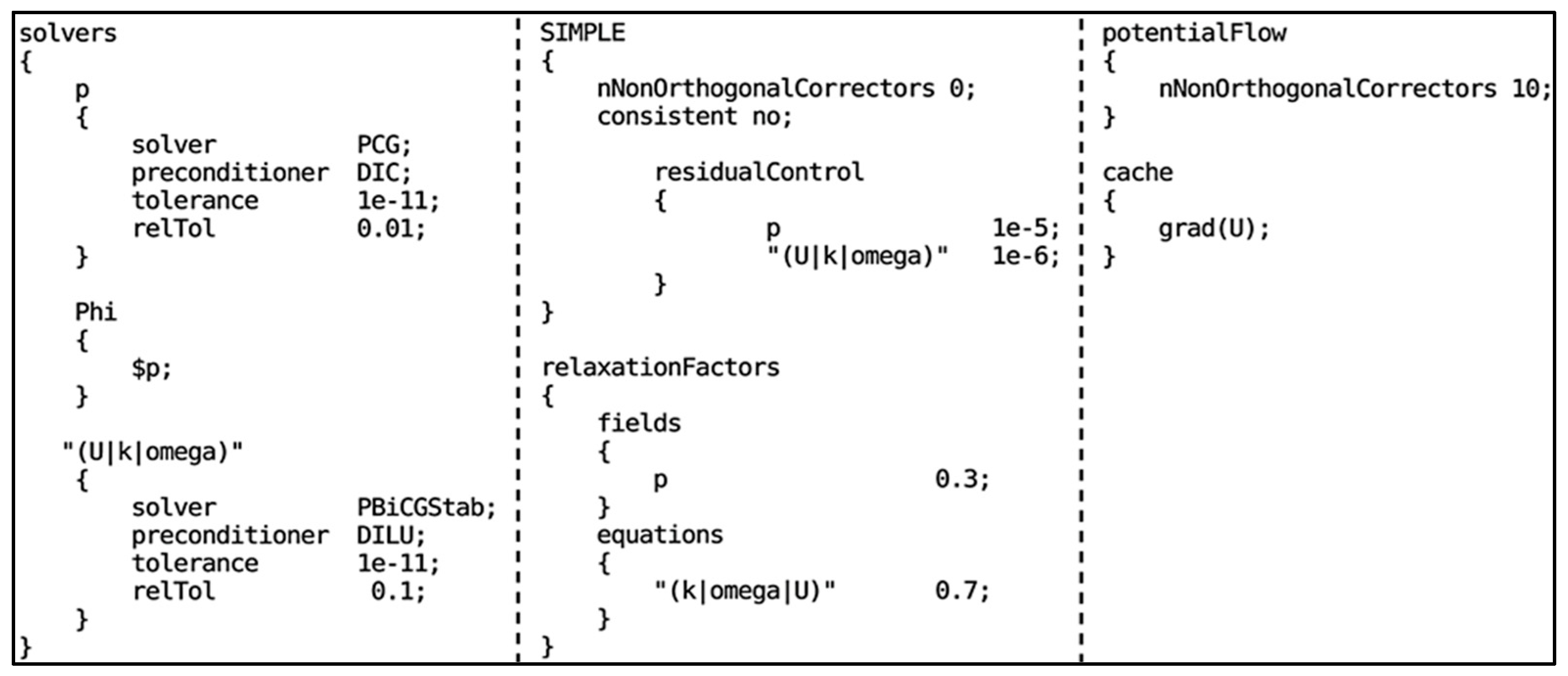
The fvSolution file of RANS simulations in the example case is shown in Figure 8. The preconditioned conjugate gradient (PCG) linear solver [72] with the diagonal-based incomplete Cholesky (DIC) preconditioner is used to solve matrices of pressure and flux. Matrices of the rest parameters are solved by the preconditioned bi-conjugate gradient (PBiCGStab) linear solver [73] with the diagonal-based incomplete lower-upper (DILU) preconditioner. Both solvers have a solving tolerance of 1 × 10⁻¹¹. The SIMPLE algorithm [74] is used to perform the pressure-velocity coupling. In OpenFOAM, the simpleFoam solver can adopt both the SIMPLE algorithm and the SIMPLEC algorithm [75], where the former is selected by setting the consistent variable to a false value. Before running the simpleFoam solver, the potentialFoam solver is run for 10 iterations to initialize velocity, pressure, and flux fields. The gradient of the velocity field is cached to speed up the solver.
The fvSolution file of the URANS simulations in the example case is shown in Figure 9. For URANS simulations in the example case, the pimpleFoam solver is utilized, which adopts a hybrid algorithm of PISO [76] and SIMPLE. Configurations of linear solvers in the URANS simulation are similar to those in the RANS simulations, except that the relative tolerance of these linear solvers is set to be zero at the final iteration of the outer corrector for each parameter. The value of nCorrectors is set to be 2, which is within the recommended values (1 to 3) in the OpenFOAM user guide v9 [67]. Although the user guide also suggests that the nOuterCorrectors take a value from 50 to 1000, we use a larger value (2000) to ensure that the outer correction converges. The outer correction iterations work like the SIMPLE iterations, and so under-relaxation factors are applied.

8. Parallel Configurations—decomposeParDict

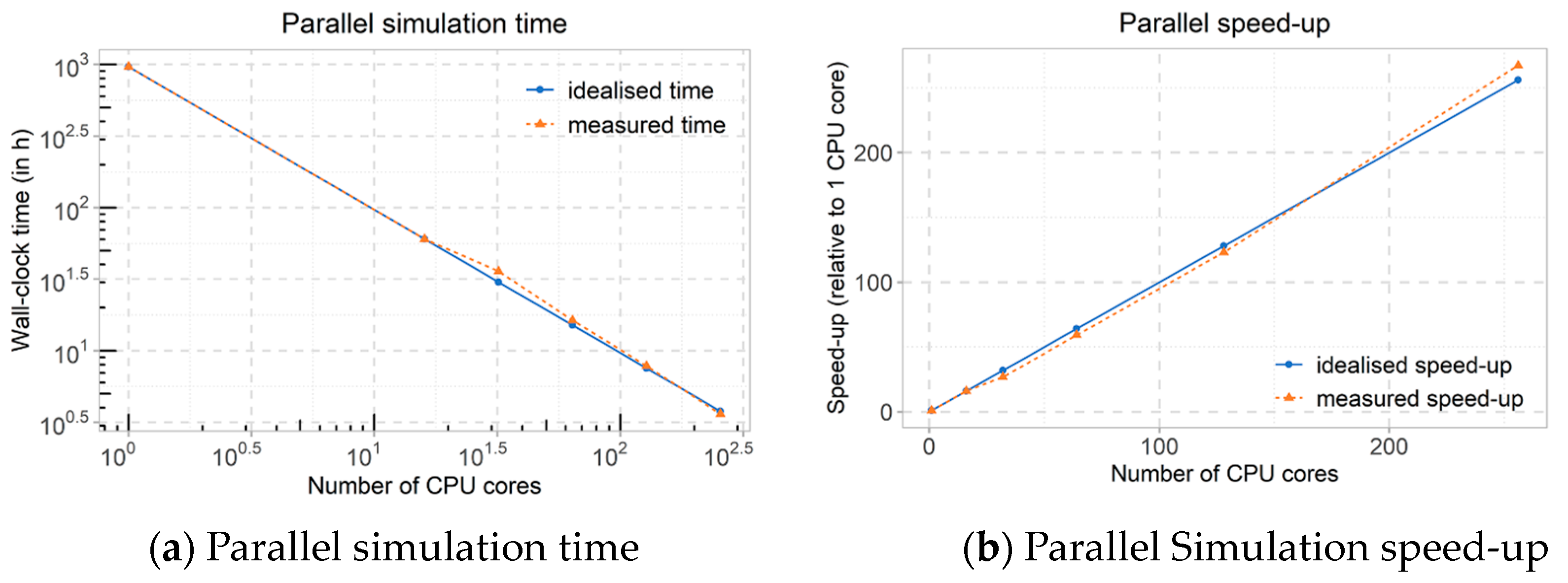
Simulations in this example case would likely have cell counts of over 30 million, and so running simulations in parallel is necessary. The SCOTCH algorithm [77] should be selected in the decomposeParDict file to perform mesh decomposition. For our research applications, simulations were performed on 128 CPU cores (Intel Xeon Gold 6148 processors running at 2.4 GHz) of the Irish Centre for High-End Computing (ICHEC) Kay server. For commercial applications, alternative processing capability would need to be sourced. The use of 128 CPU cores is not random but a decision based on a strong scalability test on the server where the RANS simulation is run for 6000 iterations with different numbers of CPU cores. Details of these tests are summarized in Table 2. Figure 8 shows the simulation time and the simulation speed-up. In an ideal condition, the simulation should scale linearly, i.e., using 64 CPU cores should speed up the simulation 64 times. However, Figure 10b shows that using 64 or fewer cores does not reach the idealized speed-up rate. On the contrary, a super-linear parallel speed-up is seen, where using 256 cores speeds up the simulation by a factor of 267 versus using 1 CPU core. This can be explained by the cache effects in parallel computing [78]. Similar super-linear parallel speed-up due to the cache effects was also reported in simulations by Cardiff et al. [79]. Although the computing time of the simulation using 256 cores is over 3 h shorter than using 128 cores, the queueing time on the server is significantly increased. Therefore, using 128 CPU cores provides a balance between the queueing time and the computing time for the example case.

9. Mesh Sensitivity Study

As mentioned in Section 3, the mesh quality can affect the accuracy of simulation results. Hence, a mesh sensitivity study should be performed. Typically, this involves creating a coarser mesh and a finer mesh, running the simulations for each, and comparing results. Ideally, the finer mesh will give results that are the same as the starting mesh. This indicates that there is no benefit to using the finer mesh and it would be wasteful of computational effort. Ideally, the coarser mesh will give different results, indicating that it is not accurate enough. In doing this, one can have confidence that the chosen mesh is appropriate for the task at hand. Figure 11 presents four meshes for our example case study to represent a mesh sensitivity study. The mesh described in Section 3 is represented here in Figure 11c.
The coarse mesh in Figure 11a has a background mesh where cells within have a length of 0.1 m. Based on this background mesh, refinement of six levels was applied, where two buffer layers were added between adjacent levels. The smallest cell within the coarse mesh has a thickness of 1.5625 × 10⁻³ m, which corresponds to a y+ value of approximately 10. The medium mesh (Figure 11b) has a background mesh that is one level finer than the coarse mesh. To better capture the flow characteristics in the region that is close to the geometry, a refinement box was used, where cells were firstly refined to level 4 and then refined to level 6 at the surface of the geometry. The smallest cell within the medium mesh has a thickness of approximately 7.8125 × 10⁻⁴ m, which corresponds to a y+ value of approximately 5. The finer mesh in Figure 11d has a similar scheme as the fine mesh (Figure 11c), except that it has a finer background mesh where cells within have a thickness of 0.03 m. Accordingly, the y+ value of the finer mesh (approximately 0.25) is smaller than that of the fine mesh (approximately 0.45). Table 3 shows the cell counts of these meshes. It should be noted that with different configurations of the angle of attack, cell counts slightly vary for each mesh.
It is straightforward to perform a mesh sensitivity study in simulations using 2D structured meshes, where they can compare parameters calculated from simulations using meshes of different mesh density, i.e., different cell counts. However, for modelling wind effects on bridges where meshes should be 3D and unstructured, the cell count is no longer suitable to illustrate the mesh density. This is because meshes with a similar cell count can have very different cell sizes at the near-wall region, which is of interest in this type of study when using different refining schemes. Here, average cell sizes at the patch of interest (the bridge) should be used as an indicator of mesh density. Figure 12 demonstrates a mesh sensitivity study using the four meshes.
Aerodynamic coefficients are calculated using the presented four meshes and corresponding numerical configurations in the following sections. It can be found that the use of the coarse mesh and medium mesh can determine results that are up to over 80% different from the results determined using the finer mesh. In contrast, there is no appreciable change in results between using the fine mesh and the finer mesh where relative differences are below 2%. In addition, the use of the finer mesh requires more than three times the computational power than the fine mesh. Therefore, based on the results of the mesh sensitivity study, the fine mesh is deemed to be the suitable mesh for the study.
It should be noted that only four mesh schemes are presented here to provide readers with a sense of how a suitable mesh is developed using snappyHexMesh in OpenFOAM. However, in reality, it is likely that far more than four meshes would be developed and analyzed before choosing a final mesh.

10. Post Processing

10.1. Aerodynamic Force Coefficients

During each SIMPLE iteration and PISO or PIMPLE time step, aerodynamic forces, namely the drag force (Fx), lift force (Fz), and pitching moment (My), are calculated using the force function.
As this is an incompressible case, the air density (at 15 °C) is specified with a constant value of 1.225 kg/m3. The porosity variable is given a false value since porous effects are not considered in bridge deck aerodynamic studies. The CofR variable defines the center of rotation for calculating the pitching moment.
Output of the force function is stored in the postprocessing/directory, where both viscous and pressure parts of drag forces (Fx), lift forces (Fz), and pitching moments (My) are recorded at each time step and SIMPLE iteration in URANS simulations and RANS simulations, respectively. Summations of the viscous and pressure parts of each force should be taken to determine their full values. Then, aerodynamic coefficients of the bridge deck, namely the drag coefficient (CFx), lift coefficient (CFz), and moment coefficient (CMy), are calculated in Equations (5)–(7) based on aerodynamic forces:
CFx = 2 Fx/ρU2 HL
CFz = 2 Fz/ρU2 BL
CMy = 2 My/ρU2 B^2 L
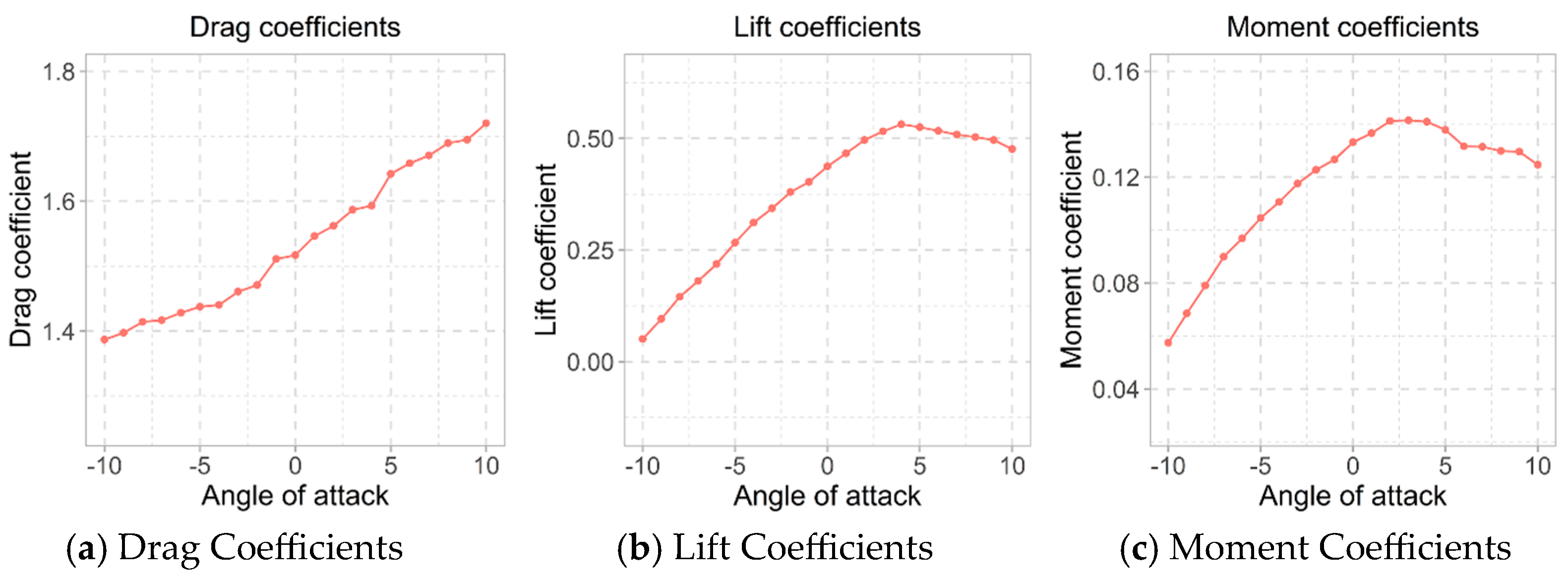
where Fx, Fz, My are drag force, lift force, and pitching moment, respectively; ρ is the density of the air, which is 1.225 kg/m3 and corresponds to the temperature at 15 °C; U is the reference velocity (P1); B is the effective width of the bridge deck (P4); H is the depth of the bridge deck (P5); and L is the span of the bridge deck (P6). Figure 13 shows the sample aerodynamic coefficients that would be calculated from the simulation results. These coefficients are essential to bridge design, especially in the topological optimization of bridge decks.

10.2. Visualization

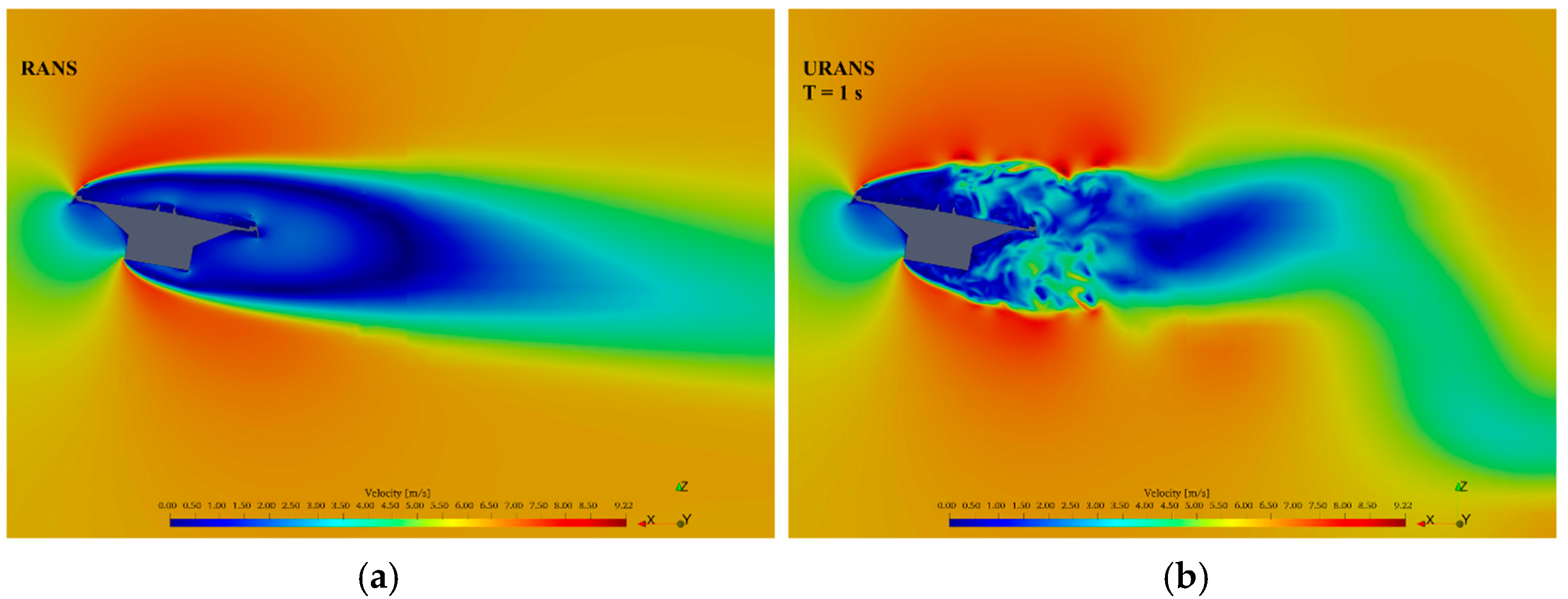
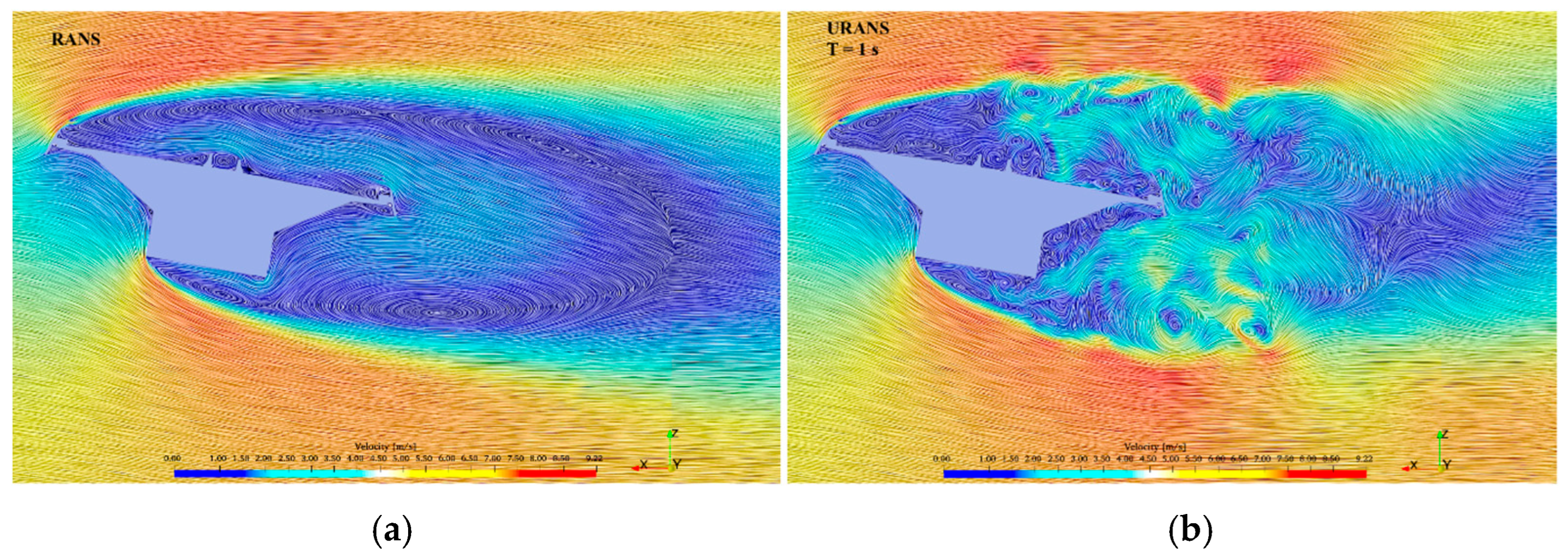
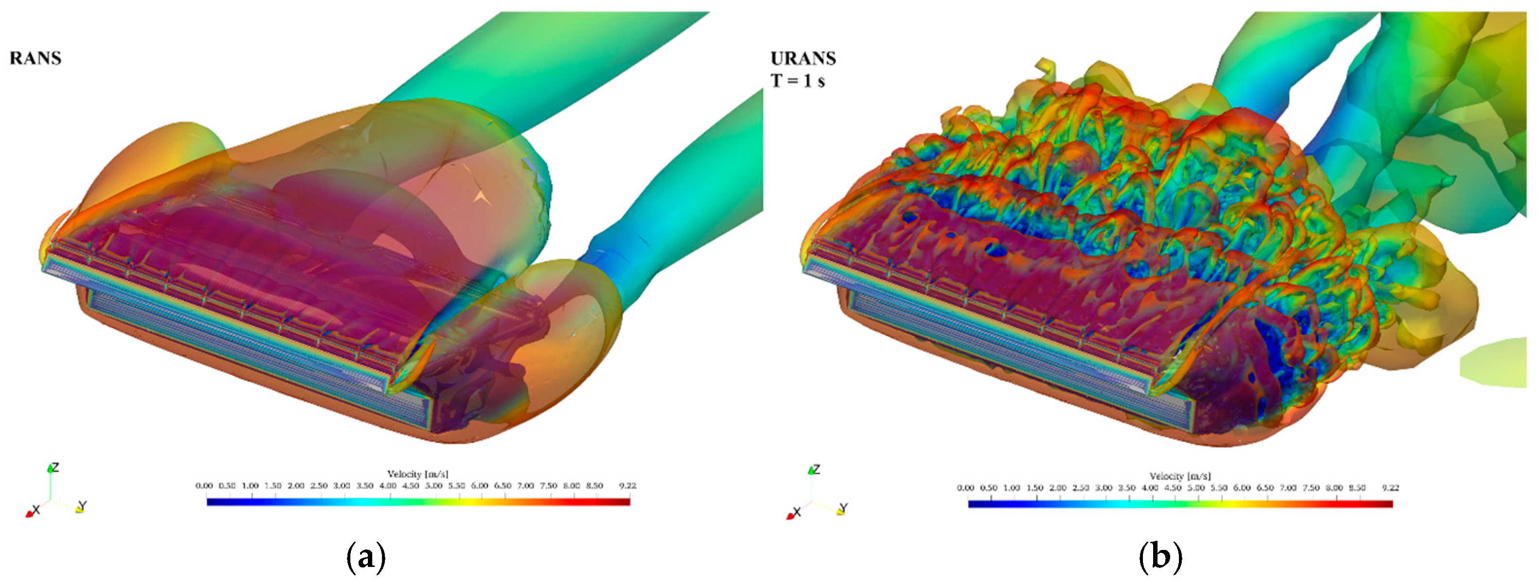
Apart from the quantitative results that can be calculated using the various functions, simulation results can also be visualized. The authors recommended that this be done in ParaView [80]. There are many ways to visualize results. Figure 14a,b shows typical velocity plots that would be generated from our example case of RANS and URANS simulations, respectively. To illustrate the flow circulations, the line integral convolution (LIC) representation is used in Figure 15. The images clearly illustrate the simplifications of a steady-state analysis whereby the velocities appear smooth in Figure 14a and Figure 15a and more rotational in Figure 14b and Figure 15b. The URANS simulation better captures the intricacies of complex flow analysis. Figure 16 shows another parameter that bridge engineers are interested in, the wall shear stress on the bridge deck surface, where Figure 16a shows wall shear stress from a RANS simulation and Figure 16b shows that from a URANS simulation. Evidence of flow structures are present in Figure 16b that are not present in Figure 16a. Finally, using the Q-criterion, Figure 16a,b show the turbulence structures from RANS simulations and URANS simulations, respectively. The Q-criterion (Figure 17) defines vortices as areas where the vorticity magnitude is greater than the magnitude of the rate of strain.
These visualizations provide a powerful tool for bridge designers to help communicate results of wind effects on bridges. They offer an opportunity to visually demonstrate to architects, clients, planning authorities, and others involved in the design and commissioning process of new bridges the implications of one design over another. They offer a similarly useful tool for existing bridges where a variety of remediation works are being considered.

11. Validation of the Methodology

The methodology presented in this paper has been deliberately developed to be sufficiently generic so as to accommodate many types of long-span bridges while still being viable for industrial applications. It is designed to have enough detail for bridge designers to use that can also be trusted based on its implementation with two real bridges—the Queensferry Crossing in Edinburgh [22,23] and the Rose Fitzgerald Kennedy Bridge in Ireland [21,46].
Zhu et al. [23] simulated a full-scale three-dimensional CFD model of the middle span and central tower of the Queensferry Crossing that was created in OpenFOAM with the k-ω SST turbulence model. Atmospheric boundary layer inflows were configured based on wind profiles provided by a full-scale weather research and forecasting (WRF) model. CFD predictions were validated with field data, which were collected from an on-site structural health monitoring system. The simulated fluctuating wind field closely satisfied the characteristics of field data and demonstrated that the modelling approach had good potential to be used in practical bridge aerodynamic studies. Figure 18 below, reproduced from [23], shows wind velocities at a particular location estimated from CFD simulations with three different mesh refinements and verified with the field data recorded at the same location, indicating an average difference of just 10%.
Zhang et al. [46] developed a full-scale 3-dimensional CFD simulation model to replicate wind conditions at the Rose Fitzgerald Kennedy Bridge in Ireland. Wind velocities at four different points calculated by CFD simulations were compared with corresponding data collected from SHM field measurements. The calculated time-averaged wind velocities at four different locations on the bridge were shown to have relative differences of less than 10% to the measured wind velocities by anemometers 90% of the time. Figure 19, reproduced from [46], demonstrates these results for one of the sensors. In this example, the average relative difference within the comparison is 6%, and the underlying behavior within the time history of the wind velocity is generally predicted by the CFD simulations.

12. Conclusions

In this paper, a workflow is presented to develop CFD models in OpenFOAM to assess wind effects on long-span bridges that are computationally viable for industrial applications. Detailed configurations and corresponding considerations are described within each step. Comments on the validation of this methodology with field data collected from two-long span bridges are provided. By adopting this workflow, OpenFOAM can be used as an efficient tool that provides bridge engineers with key parameters in their design of long-span bridges against wind effects. In addition, the open-source nature makes this tool more affordable compared to commercial alternatives. Therefore, it can be foreseen that OpenFOAM will have an increasingly large community among civil engineering users.

Author Contributions

Conceptualization, R.M., J.K. and Y.Z.; methodology, J.K., P.C. and Y.Z.; software, Y.Z.; validation, Y.Z.; formal analysis, Y.Z.; investigation, Y.Z.; writing—original draft preparation, Y.Z.; writing—review and editing, J.K. and P.C.; visualization, Y.Z.; supervision, J.K. and P.C.; project administration, J.K.; funding acquisition, J.K. All authors have read and agreed to the published version of the manuscript.

Funding

This research was funded by China Scholarship Council, grant number 201808300003. The field measurement data were pro-vided by Transport Infrastructure Ireland (TII). Information on the terrain at the site of the Rose Fitzgerald Kennedy Bridge was provided by Ordnance Survey Ireland (OSI) mapping agency.

Data Availability Statement

No new data were created or analyzed in this study. Data sharing is not applicable to this article.

Conflicts of Interest

The authors declare no conflict of interest. The funders had no role in the design of the study; in the collection, analyses, or interpretation of data; in the writing of the manuscript; or in the decision to publish the results.

References

  1. Simiu, E.; Yeo, D. Wind Effects on Structures: Modern Structural Design for Wind; Wiley Online Library: Hoboken, NJ, USA, 2019. [Google Scholar]
  2. Xu, Y.; Sun, D.; Ko, J.; Lin, J. Fully coupled buffeting analysis of Tsing Ma suspension bridge. J. Wind. Eng. Ind. Aerodyn. 2000, 85, 97–117. [Google Scholar] [CrossRef]
  3. Scanlan, R.H.; Tomko, J.J. Airfoil and bridge deck flutter derivatives. J. Eng. Mech. Div. 1971, 97, 1717–1737. [Google Scholar] [CrossRef]
  4. Wu, T.; Kareem, A. An overview of vortex-induced vibration (VIV) of bridge decks. Front. Archit. Civ. Eng. 2012, 6, 335–347. [Google Scholar] [CrossRef]
  5. Ge, Y.; Lin, Z.; Cao, F.; Pang, J.; Xiang, H. Investigation and prevention of deck galloping oscillation with computational and experimental techniques. J. Wind. Eng. Ind. Aerodyn. 2002, 90, 2087–2098. [Google Scholar] [CrossRef]
  6. Ni, Y.; Wang, X.; Chen, Z.; Ko, J. Field observations of rain-wind-induced cable vibration in cable-stayed Dongting Lake Bridge. J. Wind. Eng. Ind. Aerodyn. 2007, 95, 303–328. [Google Scholar] [CrossRef]
  7. Gao, D.; Chen, W.; Eloy, C.; Li, H. Multi-mode responses, rivulet dynamics, flow structures and mechanism of rain-wind induced vibrations of a flexible cable. J. Fluids Struct. 2018, 82, 154–172. [Google Scholar] [CrossRef]
  8. Sukamta; Guntorojati, I. Fariduzzaman Flutter analysis of cable stayed bridge. Procedia Eng. 2017, 171, 1173–1177. [Google Scholar] [CrossRef]
  9. Mei, H.; Wang, Q.; Liao, H.; Fu, H. Improvement of flutter performance of a streamlined box girder by using an upper central stabilizer. J. Bridg. Eng. 2020, 25, 04020053. [Google Scholar] [CrossRef]
  10. Niu, H.; Zhu, J.; Chen, Z.; Zhang, W. Dynamic performance of a slender truss bridge subjected to extreme wind and traffic loads considering 18 flutter derivatives. J. Aerosp. Eng. 2019, 32, 04019082. [Google Scholar] [CrossRef]
  11. Li, S.; Li, M.; Larose, G.L. Aerodynamic admittance of streamlined bridge decks. J. Fluids Struct. 2018, 78, 1–23. [Google Scholar] [CrossRef]
  12. Anas, S.; Alam, M.; Umair, M. Experimental and Numerical Investigations on Performance of Reinforced Concrete Slabs under Explosive-Induced Air-Blast Loading: A State-of-the-Art Review. In Structures; Elsevier: Amsterdam, The Netherlands, 2021; Volume 31, pp. 428–461. [Google Scholar] [CrossRef]
  13. Helgedagsrud, T.A.; Bazilevs, Y.; Mathisen, K.M.; Øiseth, O.A. Computational and experimental investigation of free vibration and flutter of bridge decks. Comput. Mech. 2019, 63, 121–136. [Google Scholar] [CrossRef]
  14. Jing, H.; He, X.; Wang, Z. Numerical modeling of the wind load of a two-dimensional cable model in rain–wind-induced vibration. J. Fluids Struct. 2018, 82, 121–133. [Google Scholar] [CrossRef]
  15. Xu, F.; Zhang, Z. Free vibration numerical simulation technique for extracting flutter derivatives of bridge decks. J. Wind. Eng. Ind. Aerodyn. 2017, 170, 226–237. [Google Scholar] [CrossRef]
  16. Zhang, T.; Sun, Y.; Li, M.; Yang, X. Experimental and numerical studies on the vortex-induced vibration of two-box edge girder for cable-stayed bridges. J. Wind. Eng. Ind. Aerodyn. 2020, 206, 104336. [Google Scholar] [CrossRef]
  17. Selvam, R.P. Computational Fluid Dynamics for Wind Engineering; John Wiley & Sons: Hoboken, NJ, USA, 2022. [Google Scholar] [CrossRef]
  18. Kuroda, S. Numerical simulation of flow around a box girder of a long span suspension bridge. J. Wind. Eng. Ind. Aerodyn. 1997, 67–68, 239–252. [Google Scholar] [CrossRef]
  19. Murakami, S.; Mochida, A. 3-D numerical simulation of airflow around a cubic model by means of the k-ϵ model. J. Wind Eng. Ind. Aerodyn. 1988, 31, 283–303. [Google Scholar] [CrossRef]
  20. Selvam, R.P.; Tarini, M.J.; Larsen, A. Computer modelling of flow around bridges using LES and FEM. J. Wind. Eng. Ind. Aerodyn. 1998, 77–78, 643–651. [Google Scholar] [CrossRef]
  21. Zhang, Y.; Cardiff, P.; Cahill, F.; Keenahan, J. Assessing the Capability of Computational Fluid Dynamics Models in Rep-licating Wind Tunnel Test Results for the Rose Fitzgerald Kennedy Bridge. CivilEng 2021, 2, 1065–1090. [Google Scholar] [CrossRef]
  22. Zhu, L.; McCrum, D.; Keenahan, J. Capability analysis of computational fluid dynamics models in wind shield study on Queensferry Crossing, Scotland. In Proceedings of the Institution of Civil Engineers-Bridge Engineering; Thomas Telford Ltd.: London, UK, 2022; pp. 1–13. [Google Scholar] [CrossRef]
  23. Zhu, L.; McCrum, D.; Sweeney, C.; Keenahan, J. Full-scale computational fluid dynamics study on wind condition of the long-span Queensferry Crossing Bridge. J. Civ. Struct. Health Monit. 2023, 13, 615–632. [Google Scholar] [CrossRef]
  24. Tang, H.; Li, Y.; Shum, K.; Xu, X.; Tao, Q. Non-uniform wind characteristics in mountainous areas and effects on flutter performance of a long-span suspension bridge. J. Wind. Eng. Ind. Aerodyn. 2020, 201, 104177. [Google Scholar] [CrossRef]
  25. Bruno, L.; Coste, N.; Fransos, D. Simulated flow around a rectangular 5:1 cylinder: Spanwise iscretization effects and emerging flow features. J. Wind. Eng. Ind. Aerodyn. 2012, 104–106, 203–215. [Google Scholar] [CrossRef]
  26. Bruno, L.; Fransos, D.; Coste, N.; Bosco, A. 3D flow around a rectangular cylinder: A computational study. J. Wind. Eng. Ind. Aerodyn. 2010, 98, 263–276. [Google Scholar] [CrossRef]
  27. Bruno, L.; Salvetti, M.V.; Ricciardelli, F. Benchmark on the Aerodynamics of a Rectangular 5:1 Cylinder: An overview after the first four years of activity. J. Wind. Eng. Ind. Aerodyn. 2014, 126, 87–106. [Google Scholar] [CrossRef]
  28. Mannini, C.; Marra, A.M.; Pigolotti, L.; Bartoli, G. The effects of free-stream turbulence and angle of attack on the aerodynamics of a cylinder with rectangular 5:1 cross section. J. Wind. Eng. Ind. Aerodyn. 2017, 161, 42–58. [Google Scholar] [CrossRef]
  29. Patruno, L.; Ricci, M.; de Miranda, S.; Ubertini, F. Numerical simulation of a 5:1 rectangular cylinder at non-null angles of attack. J. Wind. Eng. Ind. Aerodyn. 2016, 151, 146–157. [Google Scholar] [CrossRef]
  30. Mannini, C.; Šoda, A.; Schewe, G. Unsteady RANS modelling of flow past a rectangular cylinder: Investigation of Reynolds number effects. Comput. Fluids 2010, 39, 1609–1624. [Google Scholar] [CrossRef]
  31. Fransos, D.; Bruno, L. Edge degree-of-sharpness and free-stream turbulence scale effects on the aerodynamics of a bridge deck. J. Wind. Eng. Ind. Aerodyn. 2010, 98, 661–671. [Google Scholar] [CrossRef]
  32. Nieto, F.; Montoya, M.C.; Hernández, S.; Kusano, I.; Casteleiro, A.; Álvarez, A.J.; Jurado, J.; Fontán, A. Aerodynamic and aeroelastic responses of short gap twin-box decks: Box geometry and gap distance dependent surrogate based design. J. Wind. Eng. Ind. Aerodyn. 2020, 201, 104147. [Google Scholar] [CrossRef]
  33. Cid Montoya, M.; Hernández, S.; Nieto, F. Shape optimization of streamlined decks of cable-stayed bridges considering aeroelastic and structural constraints. J. Wind Eng. Ind. Aerodyn. 2018, 177, 429–455. [Google Scholar] [CrossRef]
  34. Montoya, M.C.; Nieto, F.; Hernández, S.; Kusano, I.; Álvarez, A.; Jurado, J. CFD-based aeroelastic characterization of streamlined bridge deck cross-sections subject to shape modifications using surrogate models. J. Wind. Eng. Ind. Aerodyn. 2018, 177, 405–428. [Google Scholar] [CrossRef]
  35. Álvarez, A.; Nieto, F.; Nguyen, D.; Owen, J.; Hernández, S. 3D LES simulations of a static and vertically free-to-oscillate 4:1 rectangular cylinder: Effects of the grid resolution. J. Wind. Eng. Ind. Aerodyn. 2019, 192, 31–44. [Google Scholar] [CrossRef]
  36. Mannini, C.; Sbragi, G.; Schewe, G. Analysis of self-excited forces for a box-girder bridge deck through unsteady RANS simulations. J. Fluids Struct. 2016, 63, 57–76. [Google Scholar] [CrossRef]
  37. Nguyen, D.T.; Hargreaves, D.M.; Owen, J.S. Vortex-induced vibration of a 5:1 rectangular cylinder: A comparison of wind tunnel sectional model tests and computational simulations. J. Wind. Eng. Ind. Aerodyn. 2018, 175, 1–16. [Google Scholar] [CrossRef]
  38. Nieto, F.; Owen, J.; Hargreaves, D.; Hernández, S. Bridge deck flutter derivatives: Efficient numerical evaluation exploiting their interdependence. J. Wind. Eng. Ind. Aerodyn. 2015, 136, 138–150. [Google Scholar] [CrossRef]
  39. EN Eurocode 1—Actions on Structures—Part 1–4: General Actions—Wind Actions—Irish National Annex; CEN: Paris, France, 2010.
  40. CEN/TC 250. In Eurocode 1—Actions on Structures—Part 1–4: General Actions—Wind Actions. Third Draft: October 2019 Version; CEN: Paris, France, 2019.
  41. Keenahan, J. (Ed.) Reamonn MacReamoinn. CFD Development in Bridge Engineering, 2022. [Google Scholar]
  42. Zhang, Y.; Cardiff, P.; Keenahan, J. Wind-Induced Phenomena in Long-Span Cable-Supported Bridges: A Comparative Review of Wind Tunnel Tests and Computational Fluid Dynamics Modelling. Appl. Sci. 2021, 11, 1642. [Google Scholar] [CrossRef]
  43. Hu, C.; Zhao, L.; Ge, Y. Mechanism of suppression of vortex-induced vibrations of a streamlined closed-box girder using additional small-scale components. J. Wind. Eng. Ind. Aerodyn. 2019, 189, 314–331. [Google Scholar] [CrossRef]
  44. Li, H.; Chen, W.-L.; Xu, F.; Li, F.-C.; Ou, J.-P. A numerical and experimental hybrid approach for the investigation of aer-odynamic forces on stay cables suffering from rain-wind induced vibration. J. Fluids Struct. 2010, 26, 1195–1215. [Google Scholar] [CrossRef]
  45. Szabo, G.; Gyorgyi, J.; Kristof, G. Advanced flutter simulation of flexible bridge decks. Coupled Syst. Mech. 2012, 1, 133–154. [Google Scholar] [CrossRef]
  46. Zhang, Y.; Sweeney, C.; Cardiff, P.; Cahill, F.; Keenahan, J. Quantifying the Impact of Bridge Geometry and Surrounding Terrain: Wind Effects on Bridges. In Proceedings of the Institution of Civil Engineer: Bridge Engineering; Thomas Telford Ltd.: London, UK, 2023; pp. 1–18. [Google Scholar] [CrossRef]
  47. Ferziger, J.H.; Peric, M. Computational Methods for Fluid Dynamics; Springer Science & Business Media: Berlin, Germany, 2012. [Google Scholar]
  48. Lee, H.; Moon, J.; Chun, N.; Lee, H.E. Effect of beam slope on the static aerodynamic response of edge-girder bridge-deck. Wind Struct. 2017, 25, 157–176. [Google Scholar]
  49. Liu, L.; Zhang, L.; Wu, B.; Chen, B.; Aecom, P. Effect of Accessory Attachment on Static Coefficients in a Steel Box Girder for Long—Span Suspension Bridges. J. Eng. Sci. Technol. Rev. 2017, 10, 68–83. [Google Scholar] [CrossRef]
  50. Kusano, I.; Jakobsen, J.B.; Snæbjörnsson, J.T. CFD simulations of a suspension bridge deck for different deck shapes with railings and vortex mitigating devices. IOP Conf. Ser. Mater. Sci. Eng. 2019, 700, 012003. [Google Scholar] [CrossRef]
  51. Menter, F.R.; Kuntz, M.; Langtry, R. Ten years of industrial experience with the SST turbulence model. Turbul. Heat Mass Transf. 2003, 4, 625–632. [Google Scholar]
  52. Anina, H.; Rüdiger, H.; Stanko, B. Numerical simulations and experimental validations of force coefficients and flutter derivatives of a bridge deck. J. Wind Eng. Ind. Aerodyn. 2015, 144, 172–182. [Google Scholar]
  53. Zhang, H.; Xin, D.; Ou, J. Wake control using spanwise-varying vortex generators on bridge decks: A computational study. J. Wind. Eng. Ind. Aerodyn. 2019, 184, 185–197. [Google Scholar] [CrossRef]
  54. Chen, X.; Qiu, F.; Tang, H.; Li, Y.; Xu, X. Effects of secondary elements on vortex-induced vibration of a streamlined box girder. KSCE J. Civ. Eng. 2021, 25, 173–184. [Google Scholar] [CrossRef]
  55. Könözsy, L. The k-ω Shear-Stress Transport (SST) Turbulence Model. In A New Hypothesis on the Anisotropic Reynolds Stress Tensor for Turbulent Flows: Volume I: Theoretical Background and Development of an Anisotropic Hybrid k-omega Shear-Stress Transport/Stochastic Turbulence Model; Springer: Berlin/Heidelberg, Germany, 2019; pp. 57–66. [Google Scholar]
  56. Lien, F.-S.; Kalitzin, G. Computations of transonic flow with the v2–f turbulence model. Int. J. Heat Fluid Flow 2001, 22, 53–61. [Google Scholar] [CrossRef]
  57. Langtry, R.B.; Menter, F.R. Correlation-based transition modeling for unstructured parallelized computational fluid dy-namics codes. AIAA J. 2009, 47, 2894–2906. [Google Scholar]
  58. Cécora, R.-D.; Eisfeld, B.; Probst, A.; Crippa, S.; Radespiel, R. Differential Reynolds stress modeling for aeronautics. AIAA J. 2015, 53, 739–755. [Google Scholar] [CrossRef]
  59. Smagorinsky, J. General circulation experiments with the primitive equations: I. The basic experiment. Mon. Weather Rev. 1963, 91, 99–164. [Google Scholar] [CrossRef]
  60. Spalart, P.R. Comments on the Feasibility of LES for Wings and on the Hybrid RANS/LES Approach. In Proceedings of the First AFOSR International Conference on DNS/LES, Ruston, LA, USA, 4–8 August 1997; pp. 137–147. [Google Scholar]
  61. Solidworks; Dessault Systemes: Vélizy-Villacoublay, France, 2019.
  62. FreeCAD. 2016.
  63. An Introduction to ANSYS Fluent 2021; SDC Publications: Mission, KS, USA, 2021.
  64. Geuzaine, C.; Remacle, J.-F. Gmsh: A 3-D finite element mesh generator with built-in pre- and post-processing facilities. Int. J. Numer. Methods Eng. 2009, 79, 1309–1331. [Google Scholar] [CrossRef]
  65. Tominaga, Y.; Mochida, A.; Yoshie, R.; Kataoka, H.; Nozu, T.; Yoshikawa, M.; Shirasawa, T. AIJ guidelines for practical applications of CFD to pedestrian wind environment around buildings. J. Wind Eng. Ind. Aerodyn. 2008, 96, 1749–1761. [Google Scholar] [CrossRef]
  66. Franke, J.; Hellsten, A.; Schlünzen, H.; Carissimo, B. Best Practice Guideline for the CFD Simulation of Flows in the Urban Environment. COST Action 732: Quality Assurance and Improvement of Microscale Meteorological Models (2007). In Proceedings of the 11th Conference on Harmonisation within Atmospheric Dispersion Modelling for Regulatory Purposes, Hamburg, Germany, May 2007. [Google Scholar]
  67. Greenshields, C.J. OpenFOAM User Guide; OpenFOAM Foundation Ltd.: London, UK, 2015; Volume 3, p. 47. [Google Scholar]
  68. Bradshaw, P.; Huang, G.P. The law of the wall in turbulent flow. Proc. R. Soc. London. Ser. A Math. Phys. Sci. 1995, 451, 165–188. [Google Scholar]
  69. Liu, F. A thorough Description of How Wall Functions are Implemented in OpenFOAM. Proceedings of CFD with OpenSource Software, 2016; Volume 34. [Google Scholar]
  70. Pinier, B.; Mémin, E.; Laizet, S.; Lewandowski, R. A model under location uncertainty to predict the mean velocity in wall bounded flows. arXiv 2018, arXiv:1812.02947. [Google Scholar]
  71. Jasak, H. Error Analysis and Estimation for the Finite Volume Method with Applications to Fluid Flows. Ph.D. Thesis, Philosophy of the University, London, UK, June 1996. [Google Scholar]
  72. Barrett, R.; Berry, M.; Chan, T.F.; Demmel, J.; Donato, J.; Dongarra, J.; Eijkhout, V.; Pozo, R.; Romine, C.; Van der Vorst, H. Templates for the Solution of Linear Systems: Building Blocks for Iterative Methods. In Society for Industrial and Applied Mathematics; SIAM: Philadelphia, PA, USA, 1994. [Google Scholar] [CrossRef]
  73. Van der Vorst, H.A. Bi-CGSTAB: A fast and smoothly converging variant of Bi-CG for the solution of nonsymmetric linear systems. SIAM J. Sci. Stat. Comput. 1992, 13, 631–644. [Google Scholar] [CrossRef]
  74. Patankar, S.V.; Spalding, D.B. A Calculation Procedure for Heat, Mass and Momentum Transfer in Three-Dimensional Parabolic Flows. In Numerical Prediction of Flow, Heat Transfer, Turbulence and Combustion; Elsevier: Amsterdam, The Netherlands, 1983; pp. 54–73. [Google Scholar]
  75. Van Doormaal, J.P.; Raithby, G.D. Enhancements of the SIMPLE method for predicting incompressible fluid flows. Numer. Heat Transf. 1984, 7, 147–163. [Google Scholar]
  76. Issa, R. Solution of the implicitly discretised fluid flow equations by operator-splitting. J. Comput. Phys. 1986, 62, 40–65. [Google Scholar] [CrossRef]
  77. Chevalier, C.; Pellegrini, F. PT-Scotch: A tool for efficient parallel graph ordering. Parallel Comput. 2008, 34, 318–331. [Google Scholar] [CrossRef]
  78. Venkatesh, T.; Sarasamma, V.; Rajalakshmy, S.; Sahu, K.C.; Govindarajan, R. Super-linear speed-up of a parallel multigrid Navier–Stokes solver on Flosolver. Curr. Sci. 2005, 88, 589–593. [Google Scholar]
  79. Cardiff, P.; Karač, A.; Ivanković, A. A large strain finite volume method for orthotropic bodies with general material ori-entations. Comput. Methods Appl. Mech. Eng. 2014, 268, 318–335. [Google Scholar]
  80. Ayachit, U. The ParaView Guide: A Parallel Visualization Application; Kitware, Inc.: Clifton Park, NY, USA, 2015. [Google Scholar]
Figure 1. An overview of the OpenFOAM workflow for bridge aerodynamic studies.
Infrastructures 08 00130 g001
Figure 2. Key elements of the modelling framework.
Infrastructures 08 00130 g002
Figure 3. The 3D geometry used in the example case.
Infrastructures 08 00130 g003
Figure 4. Bridge deck geometries with different pitching angles.
Infrastructures 08 00130 g004
Figure 5. The computational domain of the example case.
Infrastructures 08 00130 g005
Figure 6. Final mesh developed for the example case.
Infrastructures 08 00130 g006
Figure 7. Content of the fvSchemes file.
Infrastructures 08 00130 g007
Figure 8. An example of the fvSolution file for RANS simulations.
Infrastructures 08 00130 g008
Figure 9. An example of fvSolution file for URANS simulations.
Infrastructures 08 00130 g009
Figure 10. Parallel simulation time and speed-up.
Infrastructures 08 00130 g010
Figure 11. Four meshes compared in the mesh sensitivity study.
Infrastructures 08 00130 g011aInfrastructures 08 00130 g011b
Figure 12. Results of the mesh sensitivity study.
Infrastructures 08 00130 g012
Figure 13. Aerodynamic coefficients of the bridge deck in the example case.
Infrastructures 08 00130 g013
Figure 14. Velocity plot on the central cross-section of the bridge deck. (a) Velocity plot of a RANS simulation. (b) Velocity plot of a URANS simulation.
Infrastructures 08 00130 g014
Figure 15. LIC representation of the velocity plot on the central cross-section of the bridge deck. (a) LIC representation of the velocity plot of a RANS simulation. (b) LIC representation of the velocity plot of a URANS simulation.
Infrastructures 08 00130 g015
Figure 16. Wall shear stress plot on the bridge deck surface. (a) Wall shear stress on the bridge deck surface of a RANS simulation. (b) Wall shear stress on the bridge deck surface of a URANS simulation.
Infrastructures 08 00130 g016
Figure 17. Turbulence structures illustrated by the Q-criterion. (a) Turbulence structures in a RANS simulation. (b) Turbulence structures in a URANS simulation.
Infrastructures 08 00130 g017
Figure 18. Effects of changes in mesh refinement level for velocities at Point CW on the QFC bridge, reproduced from [23].
Infrastructures 08 00130 g018
Figure 19. Comparison of wind velocity magnitudes from the field data and CFD simulations for point A on the RFK bridge, reproduced from [46].
Infrastructures 08 00130 g019
Table 1. Summary of boundary conditions applied in the example case.
Patch NameParameterType of Condition in OpenFOAMValueUnit
InletUfixedValueP1m/s
pzeroGradient-m2/s
kfixedValueP2m2/s
ωfixedValueP3s−1
νtcalculated-m2/s
OutletUinletOutlet-m/s
pfixedValue0m2/s2
kinletOutlet-m2/s2
ωinletOutlet-s−1
νtcalculated-m2/s
Side wallsUnoSlip0m/s
pzeroGradient-m2/s2
kkqRWallFunction-m2/s2
ωomegaWallFunction-s−1
νtnutkWallFunction-m2/s
BridgeUnoSlip0m/s
pzeroGradient-m2/s2
kfixedValue1 × 10m2/s2
ωomegaWallFunction-s−1
νtnutLowReWallFunction-m2/s
Table 2. Results of the strong scalability test.
Number of CPU CoresWall-Clock Time (in h)Speed-UpCells Per CPU Core
1965.28 (estimated)-33,189,094
1660.33161,937,500
3235.8826.903968,750
6416.3159.172484,375
1287.84123.023242,188
2563.61267.175121,094
Table 3. Cell counts of different meshes.
ConfigurationsCoarse MeshMedium MeshFine MeshFiner Mesh
−10°1,962,32414,607,63633,242,17085,922,392
1,973,22714,575,02033,189,09486,008,513
10°1,972,35514,608,86033,227,28986,441,092
Disclaimer/Publisher’s Note: The statements, opinions and data contained in all publications are solely those of the individual author(s) and contributor(s) and not of MDPI and/or the editor(s). MDPI and/or the editor(s) disclaim responsibility for any injury to people or property resulting from any ideas, methods, instructions or products referred to in the content.