Forecasting the Capacity of Open-Ended Pipe Piles Using Machine Learning

Abstract

Pile design is an essential component of geotechnical engineering practice, and pipe piles, in particular, are increasingly being used for the support of a variety of infrastructure projects. These piles are being used with dimensions that exceed those used in the development of the most widely used design approaches. At the same time, the growth in pile dimensions calls for the evolution of the state-of-the-art at a similar pace. The objective of this study is to provide an improved prediction of pile capacity. A database of 112 load tests on pipe piles ranging in diameter from 10 to 100 in. (0.25–2.5 m) and in length from 10 to 320 ft. (3–98 m) was employed in this study. First, design capacities were computed using four popular design methods and compared to capacities interpreted from a load test. For the employed dataset, the Revised Lambda method was found to best predict capacities of pipe piles obtained from a load test, among the four examined methods, and was thus employed as a reference standard for assessing the performance of ML methods. Next, eight ML regression models were trained to compute the capacity of pipe piles. Several trained ML models predicted capacities for the testing data set on par with the Revised Lambda method, and three were selected for further investigation. A variety of pile dimensions and soil properties were examined as input properties for ML and the trained models performed surprisingly well with only the pile dimensions used as input. In addition, ML models exhibited satisfactory diameter and length effects, which have been areas of concern for some traditional design approaches. The work thus demonstrates the feasibility of employing machine learning (ML) for determining the capacity of pipe piles. A web application was also developed as a tool for forecasting the capacity of pipe piles using ML.

1. Introduction

Open-ended pipe piles are one of the most widely used pile types in practice. These piles are being used with increasing pile diameters and lengths due to the growth in their use for support of bridge structures and high-rise buildings, along with their continued use for support of offshore structures [1]. Estimating the load-carrying capacity of a single pile is mostly being done using design methods to calculate the static design capacity and confirming the design capacity through one of many possible load testing approaches. Even though design methods are developed using certain types and dimensions of piles in certain soil conditions, they are commonly being used out of their scope and results are mostly the extrapolation of the dataset. This situation raises questions about the efficacy of the current practice for designing piles.

The growth in pile dimensions calls for the evolution of the state-of-the-art of pile design, at the same pace. A set of machine learning (ML) regression models were trained for calculating pile capacity. The ML models being used in this study are: (I) K-Nearest Neighbors Regression, (II) Support Vector Regression, (III) Decision Tree Regression, (IV) Ridge Regression, (V) Stochastic Gradient Descent Regression, (VI) Elastic Net Regression, (VII) Bayesian Ridge Regression, and (VIII) Kernel Ridge Regression.

To date, ML has been applied to a few applications in geotechnical engineering. Notably, ML was employed for a number of classification tasks, such as classification of sand [2]. The technique has also been introduced for automatic identification and classification of mineral and volcanic ash particles, spatial prediction of shallow landslides, and determining the plugging conditions of piles [3,4,5,6,7]. Application of ML in regression problems includes prediction of the swelling index of cohesive soils, estimating the pile-bearing capacity using deep neural networks, and predicting the critical buckling load of I-shaped cellular beams [8,9,10].

The performance of the ML models is compared to that of four widely used design methods, namely, the Federal Highway Administration (FHWA) Method [11,12], the United States Army Corps of Engineers (USACE) Method [13], American Petroleum Institute (API) Method [14], and the Revised Lambda Method [15]. The best-performing among these methods was used as a reference datum for assessing the performance of the developed ML models.

Performance of all approaches for forecasting the capacity was assessed by comparing the computed capacity, Q_c, to the measured capacity, Q_m, interpreted from load tests on individual piles. Measured pile capacities were recorded in the databases and interpreted from static load tests using the Original Davisson’s criterion [16]. These interpreted (measured) capacities were used without any additional alteration. APILE software was used for all calculations of pile capacity using traditional approaches [17]. ML was carried out using a scikit-learn package in Python [18]. Python scripts were utilized to create APILE input files and extract data from APILE output files. Various other scripts were also used to compare the interpreted and estimated capacities.

2. Dataset

For this study, a dataset of 112 pipe pile load tests was assembled from three different sources. Sixty-two load tests were publicly available from the FHWA Deep Foundation Load Test Database (DFLTD) Version 2.0 (v.2) [19]. Forty-eight load tests were collected from Prof. Olson’s Database [20,21,22], a private database collected by Professor Roy Olson and made available to the corresponding author. Finally, two load tests were added to the database from the Iowa Department of Transportation (Iowa DOT) Database [23]. The distribution of the length and diameters of the employed piles in this study is provided in Figure 1 below, where the piles are also labeled with a Data Quality Factor (DQF), where 5 stands for the highest quality and 1 for the lowest.

The employed dataset also included soil information to facilitate pile capacity calculations; however, some of the needed data were missing. Therefore, the research team thoroughly analyzed the data and determined the missing soil parameters using the correlations provided by the Naval Facilities (NAVFAC) Design Manual [24] and Peck et al. [25]. A detailed description of the data augmentation is provided by Rizk et al. [26]. Figure 2 shows principal soil information as a nested pie chart where the distribution of the predominant soil type is shown on the outer level, and the breakdown of the bearing soil layer on the inner chart per each predominant soil type.

3. Pile Design Methods under Consideration

Four conventional design methods were employed in this study. These methods have been chosen due to their wide acceptance in the industry and their availability in the APILE software. The performance of these four methods serves as a basis for assessing the developed ML methods. A summary of each conventional design method is provided as follows:

3.1. Federal Highway Administration (FHWA) Method

For cohesionless soils, FHWA utilizes Nordlund’s [27] method for calculating the capacity, Q_c, while the α-method proposed by Tomlinson [28] is employed for cohesive soils. Nordlund provides several charts to factor in the effects of pile taper, material, type, slenderness ratio, soil displacement, and friction angle. For the side resistance calculations, there are no maximum and minimum limits, while such limits are being employed for the tip resistance of piles. The α-method uses α reduction factors that increase with the increase in the clay’s undrained shear strength ($s_u$) to account for the decrease in adhesion between the skin of the pile and the soil, for stronger soils. Additionally, Tomlinson recommends reduction factors in mixed soil profiles to account for dragging weaker soils into stiffer layers that occur during driving, which consequently decreases the side resistance.

3.2. United States Army Corps of Engineers (USACE) Method

The USACE method theorizes that in cohesionless soil, the pile skin friction increases linearly up to a specific depth, defined as the critical depth ($D_c$), after which skin friction stays constant [13]. Critical depth depends on the pile diameter and the sand density. USACE also introduces the soil interface friction angle ($\delta$) based on the pile roughness and lateral earth pressure depending on the soil type and direction of loading (tensile or compressive). For cohesive soils, the USACE uses an α-method similar to the FHWA.

3.3. American Petroleum Institute (API) Method

The API design method was proposed for offshore platforms where determining the soil characteristics is difficult; hence, it is largely based on the visual description of soils [14]. The API design method uses a table to determine friction angles and limit skin friction values for piles in cohesionless soils based on the relative density and the soil’s classification (sand, silt, gravel). Additionally, for each soil type/density, the bearing capacity factor, $N_q$, and a limiting value on unit end-bearing, is determined. For cohesive soils, the α-method approach is once more employed.

3.4. Revised Lambda Method

Revised Lambda is typically employed for offshore application to calculate the capacity in cohesive soils where piles are frequently longer, and clays are typically normally consolidated. The Revised Lambda method was proposed by Kraft et al. [15] and offers equations to calculate the skin friction in clays only. When calculating side resistance for sand, APILE transforms the sand layer to an equivalent clay layer. APILE also computes the end-bearing in sands and clays using the API design method, which is customary practice in the United States.

4. Employed Machine Learning Models

All machine learning models employed were based on regression. Regression can be defined as a statistical method to estimate the relationship between a dependent variable to one or multiple independent variables. For a straightforward linear regression problem, one of the simplest methods is ordinary least squares regression, where the objective is to minimize the loss function, which is typically the sum of squared errors. This can be explained by the formula below:

$$Loss={\displaystyle \sum }_{i=1}^n{\left(y_i-{\displaystyle \sum }_{j=1}^p{w}_{ij}{x}_i\right)}^2$$

(1)

where y is the true value or dependent variable, w is a weighing coefficient, and x is the feature or independent variable. There are some complex situations where linear regression may not be able to represent the behavior with a linear set of functions. To overcome this problem, improved linear models, or more complex techniques such as Decision Trees, Support Vectors, and k-Nearest Neighbors are often used.

In this study, eight regression models were used to forecast the relationship between the ultimate bearing capacity of an axially loaded open-ended pipe pile and a number of pile and soil properties. These eight models were selected due to their availability in the scikit package employed, along with their popularity and simplicity. In this study, the models were restricted to the simple machine learning models. More advanced techniques such as ensemble methods or neural networks are not explored in this study because of the small size of the dataset. A description of these models is provided in scikit-learn documentation [18]. A summary is provided next.

4.1. k-Nearest Neighbors (kNN) Regression

kNN is one of the simplest and most intuitive approaches for non-parametric discrimination problems [29]. In classification tasks, the algorithm predicts the class of a data point based on majority voting, while in regression it predicts the target variable by taking the average of the (k) nearest points. The nearest neighboring points are determined based on the proximity between the points measured as a Euclidean distance. Calculating a weighted average based on the proximity is also common practice; however, for this study, k was set to 4 and weights were not assigned based on distance. In geotechnics, kNN has been applied to sand classification problems [30].

4.2. Decision Tree Regression

Decision trees are widely used in ML to produce a treelike model of decisions [31]. A tree-based algorithm works in a way that recursively partitions the data and sample space [32]. The name comes from the general practice of visualizing this partitioning in the form of a tree. In each step of the partitioning process, the test is selected in such a way to minimize the loss function, which is usually the mean squared error. For example, the method starts splitting by considering the diameter in the training data. The mean of the responses of a particular group is considered to be the prediction for the group. The objective of each split is to minimize the mean squared error. Both features and targets are supported in both categorical and continuous forms in tree-based algorithms. Decision Tree Regression has been employed in modelling the peak rotation and stability of shallow foundations [33].

4.3. Ridge Regression

Ridge Regression is a linear model that is optimized against the correlated features by assigning a penalty term to the weights w in Equation (1) [34]. This technique aims to minimize the weights and hence reduce the loss. This is an effective tool when more than one feature in a set is correlated to each other. Ridge regression has been successfully deployed for predicting the compressive strength of concrete [35].

4.4. Bayesian Ridge Regression

Bayesian Ridge Regression is a Bayesian approach to the Ridge Regression described above [17]. In the original model, the penalty term is set manually. In the Bayesian Ridge Regression model, the penalty term is treated as a random variable that follows a Gaussian Distribution. The implementation of this model requires that the initial values for the penalty terms are given and updated in order to minimize loss. Bayesian Ridge Regression was applied in a study of congestion’s impact on urban expressway safety [36].

4.5. ElasticNet Regression

ElasticNet Regression is another linear model that employs Ridge Regularization along with Lasso Regularization. Ridge Regularization, as explained for ridge regression, involves reducing the effect of the correlated features. However, Ridge Regression cannot “select” features since its coefficient never goes to zero, meaning it cannot eliminate any feature. However, Lasso Regularization can go one step further and can eliminate entirely the feature considering its collinearity, leading to autonomous feature selection [37]. However, Lasso Regularization tends to easily eliminate features, sometimes causing information loss or bias. Elastic Net Regression provides a solution for this downside by combining both Lasso and Ridge methods which allows the algorithm to create a simple model by selecting the best predictor features.

4.6. Stochastic Gradient Descent Regression (SGDR)

Gradient Descent Regression [38] is an algorithm that tries to minimize the cost function of linear regression with the predicted target being $w_i{x}_i+c$. In Gradient Descent Regression, a partial derivative of the cost function with respect to w and c are taken separately and the values for the variables in each iteration are plugged into both functions. The output of these two functions is, say, $D_c$ and $D_w$. In the next step, w and c are updated as $w_{i+1}=w_i-a\times D_{wi}$ and $c_{i+1}=c_i-a\times D_{ci}$, where a is the step size. This process is repeated until the cost function is minimized. In Stochastic Gradient Descent Regression, the process is performed on subsets of the dataset having a given batch size instead of implementing the process on the full dataset. SGDR is particularly useful when the number of samples is very large. Thus, the method is often applied for optimization of neural networks.

4.7. Support Vector Regression (SVR)

Support Vector Regression stems from the Support Vector Machines (SVM) algorithm where the objective is to find a hyperplane that separates the classes using nearby data points known as support vectors. The data points may be any features employed for analysis. SVM tries to find a hyperplane that has the maximum overall distance from its support vectors. In SVR, a new term, ε, is introduced to create a region around the function which effectively creates a tube. Next, SVR finds the flattest tube that contains most of the training dataset [39]. Finally, the flattest hyperplane that fits within the tube is deemed to best represent the target. It is important to point out that “tube” is a misnomer since SVR involves higher dimensions. SVR is useful for predicting continuous functions, while SVM is used for classification problems. Thus, SVM has been adopted for a variety of geotechnical classification applications, such as predicting the plugging condition of pipe piles [7] and for sand classification [2], while SVR has been previously employed for computing pile capacity [40].

4.8. Kernal Ridge Regression (KRR)

Kernal Ridge Regression computes the inner products between the data points instead of explicitly working with each of them [41]. The approach is used to gather kernel functions that represents the mapping of the inner products. Ridge regression is combined with the kernel approach to create a space with the relevant kernel and data, then KRR adapts a linear function to the space. The method is similar to SVR; however, the solution vector for KRR depends on all the training input. SVR uses a subset of training input by creating support vectors, and the loss function of SVR is also ε-insensitive while KRR uses squared error loss. KRR is not commonly employed in geotechnics, but it has been applied for prediction of wind speed [42] and sediment transport in open channel flow [43].

5. Analysis Methodology

ENSOFT’s APILE software was employed for the calculation of the pile capacity (Q_c) using the conventional design methods under investigation. APILE was chosen due to its popularity among practicing engineers and to rule out the possibility of calculation errors that could have been caused by manual calculations. Several Python scripts have been developed to create data files for APILE, and then after running each calculation, scraping the output file created by the software to extract (Q_c) Furthermore, additional Python scripts were developed by the authors to conduct the analyses. The calculated capacities (Q_c) were compared with the interpreted (measured) capacities from static load tests. The measured capacities (Q_m) were determined using the Original Davisson criterion [16]. To obtain a uniform datum of comparison, the normalized capacity (Q_c/Q_m) was calculated for each pile in this study. A Q_c/Q_m equal to 1 means that the calculated capacity is equal to the measured capacity, which is ideal.

Several statistical metrics were employed in this study to evaluate the performance of the design methods and the machine learning models, namely: (i) Coefficient of Determination, $R^2$; (ii) Mean Q_c/Q_m; (iii) Standard Deviation of Q_c/Q_m; (iv) Mean Absolute Error (MAE); and (v) Mean Absolute Percentage Error (MAPE). An $R^2$ with a value equal to 1 indicates that the regression analysis perfectly predicts the data, while a value of 0 indicates that the regression analysis failed in predicting any of the data. Mean Absolute Error is the division of the total absolute errors by the number of samples. Mean absolute percentage error is the sum of the ratio of absolute errors with the actual values divided by the number of samples. This is a better metric than MAE since it is unitless and gives a better insight on the accuracy of the prediction. For the Standard Deviation, Mean Absolute Error, and Mean Absolute Percentage Error, an ideal value would be 0, and the closer the values get to 0, the better the performance of the evaluated method or model.

To establish a baseline for evaluation of the efficacy of various machine learning models, the performance of the four traditional design methods was evaluated using the dataset employed in this study. The best-performing design method was then chosen as the datum of comparison for the machine learning models. Next, the dataset was divided randomly into a 70% training subset to train the machine learning models and a 30% testing subset used to evaluate their performance.

Several pile and soil properties were used for training the models, including: (1) diameter; (2) embedded length; (3) cross-sectional area; (4) circumference; (5) wall thickness; (6) predominant soil type; and (7) soil type at the toe of the pile. The models were trained in seven iterations. In the first iteration, they were trained using the diameter, then using the diameter and embedded length in the second iteration, and in every following iteration an additional feature was added as an input until the seventh iteration, where all the seven features were used to train the machine learning models.

6. Performance of Traditional Design Methods

To evaluate the performance of the four traditional design methods, the measured capacities (Q_m) were plotted versus the calculated capacities (Q_c) on a logarithmic scale in Figure 3. To facilitate the comparison, 1:1, 1:0.5, and 1:2 lines were also plotted. The statistical metrics associated with each design method are also presented in an inset table in the figure.

The FHWA design method exhibited the worst performance among the design methods, with an average Q_c/Q_m of 1.32 and a standard deviation of 1.15. It also had the highest MAE and MAPE, which suggests that the FHWA consistently over-predicts the capacity. The USACE exhibited a similar performance to the API design method with an average Q_c/Q_m of 1.11; however, the API method had a slightly better standard deviation (0.89) compared to the USACE (0.96). The API also had a better MAE and MAPE compared to the USACE and the FHWA. Contrarily, the Revised Lambda method was the most accurate with a mean Q_c/Q_m of 1.03, and the lowest scatter with a standard deviation of 0.72. It also exhibited the lowest MAE and MAPE of 771.25 and 0.51, respectively. This is consistent with the finding of previous studies that investigated the performance of the design method for LDOEPs and for other pile types [26,44]. Although the Revised Lambda was superior in comparison to the other methods, its mean absolute percentage error of 51% and a standard deviation of 0.72 suggests the method still has flaws.

It was concluded that the Revised Lambda method is the most consistent method for open-ended pipe piles with respect to the mean Q_c/Q_m, standard deviation of Q_c/Q_m, the mean absolute error (MAE), and the mean absolute percentage error (MAPE). Therefore, the Revised Lambda method was chosen as the datum of comparison for evaluating the performance of the Machine Learning models in the next phase of the study since it performed best among the examined traditional design methods for the employed dataset.

It is noteworthy that the performance of the traditional methods showed considerable weaknesses in terms of mean absolute percentage error. Previous analyses were carried out considering only the mean and the standard deviation of Q_c/Q_m; however, values larger and smaller than 1 were offsetting each other in terms of mean Q_c/Q_m, hence the performance looked much better. This analysis also shows that using both Q_c/Q_m and mean absolute percentage error provides more information when evaluating the performance of a design method.

7. Performance of Machine Learning Models

After establishing a datum for comparison from the available design methods, a total of 63 machine learning models (9 machine learning models × 7 features combination = 63 models in total) were evaluated to predict the pile capacity using pile and soil properties as input features. The performance of these models in training and in testing is presented in

Table 1. Training performance of the models with the various features.

Models	D			D & L			D, L, & A			D, L, A, & t			D, L, A, t, & Circ			D, L, A, t, Circ, & Predom. Soil			D, L, A, t, Circ, Predom. Soil, & Soil at Toe
	$\mu$†	$\sigma$‡	MAPE *	$\mu$	$\sigma$	MAPE	$\mu$	$\sigma$	MAPE	$\mu$	$\sigma$	MAPE	$\mu$	$\sigma$	MAPE	$\mu$	$\sigma$	MAPE	$\mu$	$\sigma$	MAPE
SVR	1.27	1.07	0.64	1.10	0.63	0.44	1.19	0.87	0.59	1.11	0.68	0.46	1.22	0.71	0.47	1.16	0.72	0.46	1.07	0.62	0.40
kNN	1.29	0.82	0.56	1.34	0.97	0.56	1.23	0.73	0.47	1.23	0.73	0.47	1.16	0.54	0.38	1.16	0.54	0.38	1.16	0.54	0.38
Decision Tree	1.22	0.66	0.41	1.10	0.37	0.25	1.08	0.32	0.21	1.08	0.32	0.21	1.08	0.32	0.21	1.08	0.32	0.21	1.09	0.35	0.23
Ridge Regression	1.35	1.47	0.92	0.91	1.84	1.08	0.92	1.84	1.08	1.00	1.67	1.03	1.02	1.73	1.02	0.96	1.82	1.05	0.98	1.76	1.04
SGD	1.43	1.37	0.87	1.01	1.67	1.02	0.98	1.72	1.04	1.02	1.65	1.02	1.02	1.65	1.02	1.00	1.69	1.03	1.08	1.54	0.99
Lasso	1.35	1.47	0.92	0.91	1.83	1.08	0.92	1.84	1.08	1.06	1.60	1.01	1.08	1.63	0.99	1.02	1.70	1.02	1.05	1.63	1.02
ElasticNet	1.62	1.23	0.85	1.20	1.39	0.92	1.20	1.39	0.92	1.23	1.37	0.92	1.13	1.47	0.96	1.07	1.55	0.97	1.09	1.52	0.97
Bayesian Ridge	1.38	1.42	0.90	0.95	1.75	1.04	0.98	1.72	1.03	1.05	1.60	1.00	1.03	1.62	1.01	0.99	1.70	1.03	1.02	1.63	1.01
Kernel Ridge	1.75	1.44	0.97	1.34	0.76	0.56	1.38	1.20	0.69	1.27	0.91	0.61	1.11	0.92	0.63	1.07	1.12	0.72	1.06	1.07	0.72

^† $\mu$: Mean Q_c/Q_m. ^‡ $\sigma$: Standard Deviation Q_c/Q_m. * MAPE: Mean Absolute Percentage Error.

and

Table 2. Testing performance of the models with the various features.

Models	D			D & L			D, L, & A			D, L, A, & t			D, L, A, t, & Circ			D, L, A, t, Circ, & Predom. Soil			D, L, A, t, Circ, Predom. Soil, & Soil at Toe
	$\mu$†	$\sigma$‡	MAPE *	$\mu$	$\sigma$	MAPE	$\mu$	$\sigma$	MAPE	$\mu$	$\sigma$	MAPE	$\mu$	$\sigma$	MAPE	$\mu$	$\sigma$	MAPE	$\mu$	$\sigma$	MAPE
SVR	1.16	0.85	0.60	1.13	0.72	0.51	1.05	0.57	0.44	1.15	0.78	0.56	1.16	0.79	0.57	1.21	0.70	0.54	1.10	0.64	0.51
kNN	1.14	0.96	0.53	1.74	1.49	1.05	1.53	1.20	0.79	1.53	1.20	0.79	1.14	0.66	0.47	1.14	0.66	0.47	1.14	0.66	0.47
Decision Tree	1.20	0.95	0.63	1.07	0.75	0.50	1.07	0.72	0.44	1.03	0.73	0.46	1.03	0.73	0.46	1.01	0.73	0.47	1.00	0.73	0.47
Ridge Regression	1.21	1.10	0.86	0.51	1.47	1.16	0.55	1.47	1.16	0.65	1.30	1.04	0.54	1.39	1.10	0.44	1.60	1.22	0.45	1.55	1.19
SGD	1.31	1.12	0.85	0.64	1.31	1.06	0.60	1.36	1.09	0.67	1.29	1.04	0.72	1.26	1.01	0.67	1.35	1.08	0.76	1.21	0.97
Lasso	1.21	1.10	0.86	0.51	1.47	1.16	0.55	1.47	1.16	0.72	1.21	0.96	0.62	1.28	1.01	0.50	1.51	1.17	0.52	1.43	1.12
ElasticNet	1.54	1.24	0.83	0.89	1.04	0.83	0.88	1.04	0.83	0.94	1.01	0.79	0.85	1.10	0.88	0.75	1.25	1.00	0.76	1.22	0.98
Bayesian Ridge	1.25	1.11	0.85	0.57	1.39	1.11	0.62	1.35	1.09	0.71	1.23	0.99	0.73	1.24	0.99	0.63	1.41	1.11	0.67	1.33	1.06
Kernel Ridge	1.68	1.32	0.88	1.35	0.88	0.62	1.25	0.82	0.58	1.23	0.77	0.59	1.14	0.82	0.64	1.19	1.17	0.85	1.18	1.30	0.92

^† $\mu$: Mean Q_c/Q_m. ^‡ $\sigma$: Standard Deviation Q_c/Q_m. * MAPE: Mean Absolute Percentage Error.

, respectively.

In general, it was observed that the Decision Tree model exhibited the best performance in training and testing among the evaluated models, followed by the SVR and the kNN models. Another noteworthy observation is that introducing additional features as an input improved the performance of most of the evaluated models. However, it is notable that this cannot be generalized, since some models performed worse with the introduction of an extra feature. Nevertheless, on average, using all the available pile and soil properties as input generally exhibited the best performance.

The performance of the models using everything as an input in training and testing is shown in Figure 4, along with the Revised Lambda method to facilitate the comparison. The scoring matrices for the training and testing are also shown in the inset table for each model. It can be observed that, except for the kNN, SVR, and Decision Tree, all other models exhibited an inferior performance compared to the bar set by the Revised Lambda method across all the applied metrics. In fact, all the models were too conservative in testing compared to training, except the Kernel Ridge model which was not conservative in training and testing as well. While being conservative is desirable in foundation engineering practice, the optimal outcome is to predict a capacity equal to, or as close as possible, to the measured capacity, and rely on the application of a reasonable factor of safety to ensure the safeness of the proposed design. Therefore, SDG, Elastic Net, and Ridge-type models were deemed unsuitable for the prediction of the pile capacity, and the performance of only the kNN, SVR, and Decision Tree models was further considered in the analysis.

It is noteworthy that the Decision Tree model achieved a near identical performance to the Revised Lambda method, and performed slightly better on some scoring metrics, which is encouraging. However, despite all efforts to prevent the model from overfitting, it is important to note the Decision Tree model is prone to memorizing the data and is thus not so suitable for small datasets like this study. The kNN model also deserves commendation for its consistent performance in training and in testing, as well as its slightly better performance in comparison to the Revised Lambda method on all scoring metrics except for the average Q_c/Q_m, where the kNN overpredicted the capacity by 15% on average.

8. Forecasting Pile Capacity Based Solely on Pile Dimensions

While the three chosen models were able to achieve a satisfactory performance when using all the available pile dimensions and soil properties as input features, a closer look at the importance of each feature shows that the pile properties were more important than the soil properties. This can be seen from Figure 5, where the importance of each input feature to the Decision Tree model is shown as a percentage of the total importance. This figure is created using the built-in feature importance attribute associated with the Decision Tree function in the scikit_learn package. It can be observed that the soil properties constitute a mere 12.5% of the total importance, while the pile dimensions represented 87.5% of the importance to the Decision Tree model, with the circumference and the length being the most important features with an importance of 56.5% and 18.6%, respectively. Therefore, the authors attempted to evaluate the efficacy of the best-performing models using only the pile dimensions. This would be beneficial for feasibility studies and early planning of design projects before soil investigations become available.

The efficacy of kNN, SVR, and decision tree models using only pile dimensions as an input in training and testing is shown in Figure 6, along with the Revised Lambda method to facilitate the comparison. The scoring matrices for the training and testing are also shown in the inset table for each model. Three observations can be made, where the first and most noticeable is that the performance of the kNN model remained unchanged with the exclusion of the soil properties from the input, suggesting that the model might have only relied on the pile dimensions regardless of the included soil properties. The second observation is that the performance of the SVR model deteriorated with the exclusion of the soil properties, which suggests that the model relied, to a certain degree, on the soil properties. The final observation is that the decision tree model exhibited slightly better performance when compared to its earlier performance.

Overall, this confirms the earlier finding that the pile dimensions are more important than the soil properties for the chosen models. Moreover, a simple decision tree model relying solely on the pile dimensions can achieve a similar performance to the more intricate Revised Lambda design method, which is encouraging.

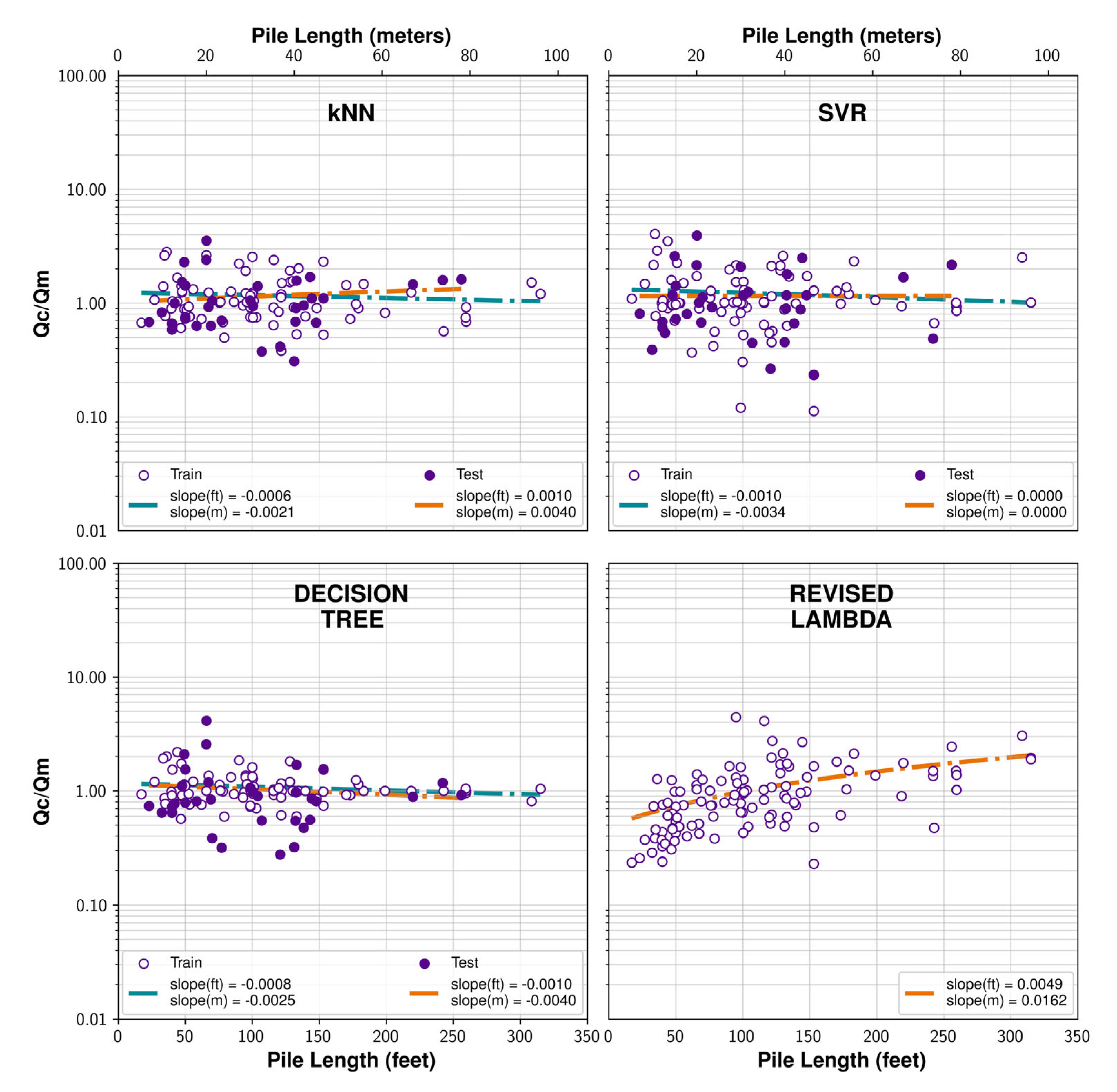
9. Effect of Diameter and Length on the Performance of the Machine Learning Models

Many design methods are notorious for exhibiting large length and diameter effects. For example, the API design method has a well-known length effect [23,26,45,46,47]. Similarly, the FHWA design method also has well-known length and diameter effects [40]. Therefore, it is important to verify the lack of diameter and length effects for the proposed machine learning models.

In our analyses, the Revised Lambda method exhibited the lowest diameter and length effects among the traditional methods explored. Therefore, it was employed as a reference standard for assessing the performance of the best-performing machine learning models. Thus, the predicted capacities in training and testing were normalized with the target variable and plotted versus the diameter and length in Figure 7 and Figure 8, respectively, along with best fit lines for both training and testing as well. It is encouraging that none of the machine learning models exhibited a strong diameter effect, and their performance is on par with that of the Revised Lambda method. With respect to length, the performance of the machine learning models was decidedly better than the Revised Lambda method, as well as the other traditional methods which are not shown here since their performance was inferior to the Revised Lambda with respect to length.

10. Web Application

A web application was developed by the authors to aid readers with exploring the use of ML for prediction of pile capacity. The application returns the forecasted pile capacity given only the diameter, length, and thickness, and the algorithm calculates the area and the circumference and uses them as the input to the Decision Tree model. The application is available at: http://cue3.engineering.nyu.edu:5020/app (accessed on 3 January 2023).

11. Limitations

This study experienced several limitations. The main limitation was the scarce number of available load tests on piles for the analysis. This number diminishes significantly when the focus is limited to only open-ended pipe piles with sufficient soil information for the capacity computation as well as load test data for capacity interpretation. Nevertheless, this is a consistent issue pertinent to data availability in the geotechnical field. Nevertheless, data availability at the present time should not discourage the adoption of ML in geotechnical engineering, especially considering the promising results of this work.

The second limitation pertains to the quality of available geotechnical data for these projects. The 48 cases pooled from the private database prepared by Professor Olson took several decades to collect and clean, and yet some cases were tagged with a low data quality factor (DQF). Moreover, the 62 cases curated from the FHWA required the experience of a practicing engineer with 15+ years of experience to carry out significant data augmentation and cleaning. However, these great efforts managed to prepare a reasonable dataset by geotechnical engineering standards which allowed for exploring the potential of machine learning in geotechnical design. The potential would be magnified with the availability of more higher quality data in the future.

12. Conclusions

This study evaluated the potential of several machine learning models to forecast the pile capacity using pile dimensions and soil properties as input. The performance of these machine learning models was compared to the performance of the best design method out of four traditional widely used methods. The analysis was carried out on a dataset of 112 open-ended pipe piles that were split into training and testing. Although the number of load tests available is barely sufficient to carry out ML analyses, several conclusions were drawn from the study, as follows:

• The Revised Lambda design method was the best among the four traditional design methods and was consequently employed as the reference of evaluation to the performance of the machine learning models.
• A variety of possible combinations of pile dimensions and soil properties was examined, and the machine learning models performed best when all available parameters were used as an input.
• Surprisingly, the most important features for predicting pile capacity were pile diameter and length, rather than the soil properties.
• Out of the evaluated models, kNN, SVR, and Decision Tree exhibited the best performance among the rest and achieved an on-par performance with the Revised Lambda method.
• The performance of these three models did not change significantly when only the pile dimensions were used as input, which is more convenient in feasibility studies and early project stages.
• The performance of the kNN model remained unchanged with the exclusion of the soil properties from the input, suggesting it did not rely on this information in the first place.
• The performance of the SVR model slightly declined with elimination of soil properties, which suggests that the model relies to a certain degree on soil information.
• The decision tree model exhibited the best performance among the evaluated models and achieved a comparable performance to the Revised Lambda method without the need for carrying out lengthy calculations.
• Machine learning models provided satisfactory diameter and length effects on par with the Revised Lambda method.

A web application was developed as a tool for practicing engineers to forecast the pile capacity using the decision tree model and only took the pile dimensions (diameter, length, and thickness) as an input. It is hoped that this application would be of use to practicing engineers.

References

- NCHRP (National Cooperative Highway Research Program). National Cooperative Highway Research Program (NCHRP) Synthesis 478: Design and Load Testing of Large Diameter Open-Ended Driven Piles; National Academies Press: Washington, DC, USA, 2015. [Google Scholar]
- Li, L.; Iskander, M. Use of Machine Learning Methods for Classification of Sand Particles. Acta Geotech. 2022, 17, 4739–4759. [Google Scholar] [CrossRef]
- Carey, C.; Boucher, T.; Mahadevan, S.; Bartholomew, P.; Dyar, M.D. Machine learning tools for mineral recognition and classification from Raman spectroscopy. J. Raman Spectrosc. 2015, 46, 894–903. [Google Scholar] [CrossRef]
- Liu, Z.; Gilbert, G.; Cepeda, J.M.; Lysdahl, A.O.K.; Piciullo, L.; Hefre, H.; Lacasse, S. Modelling of shallow landslides with machine learning algorithms. Proc. Geosci. Front. 2021, 12, 385–393. [Google Scholar] [CrossRef]
- McCoy, J.; Auret, L. Machine learning applications in minerals processing: A review. Miner. Eng. 2019, 132, 95–109. [Google Scholar] [CrossRef]
- Shoji, D.; Noguchi, R.; Otsuki, S.; Hino, H. Classification of volcanic ash particles using a convolutional neural network and probability. Sci. Rep. 2018, 8, 8111. [Google Scholar] [CrossRef]
- Kodsy, A.; Ozturk, B.; Iskander, M.G. Forecasting of Pile Plugging Using Machine Learning. Acta Geotech. 2023; In press. [Google Scholar]
- Benbouras, M.A.; Petrisor, A.-I. Prediction of Swelling Index Using Advanced Machine Learning Techniques for Cohesive Soils. Appl. Sci. 2021, 11, 536. [Google Scholar] [CrossRef]
- Benbouras, M.A.; Petrişor, A.-I.; Zedira, H.; Ghelani, L.; Lefilef, L. Forecasting the Bearing Capacity of the Driven Piles Using Advanced Machine-Learning Techniques. Appl. Sci. 2021, 11, 10908. [Google Scholar] [CrossRef]
- Ly, H.-B.; Le, T.-T.; Le, L.M.; Tran, V.Q.; Le, V.M.; Vu, H.-L.T.; Nguyen, Q.H.; Pham, B.T. Development of Hybrid Machine Learning Models for Predicting the Critical Buckling Load of I-Shaped Cellular Beams. Appl. Sci. 2019, 9, 5458. [Google Scholar] [CrossRef]
- Hannigan, P.J.; Goble, G.G.; Likins, G.E.; Rausche, F. Design and Construction of Driven Pile Foundations Reference Manual; Report No. FHWA-NHI-05-042; National Highway Institute, Federal Highway Administration, U.S. Department of Transportation: Washington, DC, USA, 2006; Volume I.
- Hannigan, P.J.; Goble, G.G.; Likins, G.E.; Rausche, F. Design and Construction of Driven Pile Foundations Reference Manual; Report No. FHWA-NHI-05-043; National Highway Institute, Federal Highway Administration, U.S. Department of Transportation: Washington, DC, USA , 2006; Volume II.
- U.S. Army Corps of Engineers (USACE). Design of Pile Foundations. Engineer Manual; U.S. Army Corps of Engineers: Washington, DC, USA, 1991; ISBN 1110-2-2906.
- American Petroleum Institute. API Recommended Practice for Planning, Designing, and Constructing Fixed Offshore Platforms, Report RP-2A; American Petroleum Institute, Production Department: Austin, TX, USA, 1993. [Google Scholar]
- Kraft, L.M., Jr.; Focht, J.A., Jr.; Amerasinghe, S.F. Friction Capacity of Piles Driven into Clay. J. Geotech. Eng. Div. 1981, 107, 1521–1541. [Google Scholar] [CrossRef]
- Davisson, M.T. High Capacity Piles. In Proceedings of the Lecture Series on Innovations in Foundation Construction, Chicago, IL, USA, January–May 1972; ASCE: Reston, VA, USA, 1972; Volume 52, pp. 81–112. [Google Scholar]
- Wang, S.T.; Arrellaga, J.A.; Vasquez, L. APILE v2019—Technical Manual: A Program for the Study of Driven Piles under Axial Loads; ENSOFT: Austin, TX, USA, 2019. [Google Scholar]
- Pedregosa, F.; Varoquaux, G.; Gramfort, A.; Michel, V.; Thirion, B.; Grisel, O.; Blondel, M.; Prettenhofer, P.; Weiss, R.; Dubourg, V.; et al. Scikit-learn: Machine Learning in Python. J. Mach. Learn. Res. 2011, 12, pp. 2825–2830.
- Petek, K.; Mitchell, R.; Ellis, H. FHWA Deep Foundation Load Test Database Version 2.0 User Manual; U.S. Department of Transportation Federal Highway Administration: McLean, VA, USA, 2016.
- Dennis, N.D.; Olson, R.E. Axial Capacity of Steel Pipe Piles in Clay. In Proceedings of the Conference on Geotechnical Practice on Offshore Engineering, Austin, TX, USA, 27–29 April 1983; ASCE: Reston, VA, USA, 1983; pp. 370–388. [Google Scholar]
- Dennis, N.D.; Olson, R.E. Axial Capacity of Steel Pipe Piles in Sand. In Proceedings of the Conference on Geotechnical Practice on Offshore Engineering, Austin, TX, USA, 27–29 April 1983; ASCE: Reston, VA, USA, 1983; pp. 389–402. [Google Scholar]
- Olson, R.; Iskander, M. Axial Load Capacity of Pipe Piles in Sands. In From Soil Behavior Fundamentals to Innovations in Geotechnical Engineering; GSP No. 233; ASCE Press: Reston, VA, USA, 2014. [Google Scholar] [CrossRef]
- Roling, M.J.; Sritharan, S.; Suleiman, M.T. Development of LRFD Procedures for Bridge Piles in Iowa Volume I: An Electronic Database for Pile Load Tests (PILOT). 2011. Available online: https://intrans.iastate.edu/app/uploads/2018/03/tr-573_lrfd_vol_1_w_cvr.pdf (accessed on 20 December 2022).
- Naval Facilities Engineering Command. Design Manual 7.01 (DM-7.01) Soil Mechanics; NAVFAC: Alexandria, VA, USA, 1986. [Google Scholar]
- Peck, R.B.; Hanson, W.E.; Thornburn, T.H. Foundation Engineering, 2nd ed.; John Wiley and Sons: New York, NY, USA, 1974. [Google Scholar]
- Rizk, A.; Kodsy, A.; Machairas, N.; Iskander, M. Efficacy of Design Methods for Predicting the Capacity of Large Diameter Open-Ended Piles ASCE Geotech. Geoenviron. Eng. J. 2022, 148, 04022078. [Google Scholar] [CrossRef]
- Nordlund, R.L. Bearing Capacity of Piles in Cohesionless Soils. J. Soil Mech. Found. Div. 1963, 89, 1–36. [Google Scholar] [CrossRef]
- Tomlinson, M.J. Foundation Design and Construction, 4th ed.; Pitman Advanced Publishing Program: Boston, MA, USA, 1980; p. 793. [Google Scholar]
- Hall, P.; Park, B.U.; Samworth, R.J. Choice of neighbor order in nearest-neighbor classification. Ann. Stat. 2008, 36, 2135–2152. [Google Scholar] [CrossRef]
- Li, L.; Iskander, M. Evaluation of Roundness Parameters in Use for Sand. J. Geotech. Geoenviron. Eng. 2021, 147, 04021081. [Google Scholar] [CrossRef]
- Friedl, M.A.; Brodley, C.E. Decision tree classification of land cover from remotely sensed data. Remote Sens. Environ. 1997, 61, 399–409. [Google Scholar] [CrossRef]
- Loh, W.-Y. Regression Trees With Unbiased Variable Selection and Interaction Detection. Stat. Sin. 2002, 12, 361–386. [Google Scholar]
- Gajan, S. Data-driven modeling of peak rotation and tipping-over stability of rocking shallow foundations using machine learning algorithms. Geotechnics 2022, 2, 781–801. [Google Scholar] [CrossRef]
- Yahya, W.B.; Olaifa, J.B. A note on ridge regression modeling techniques. Electron. J. Appl. Stat. Anal. 2014, 7, 343–361. [Google Scholar] [CrossRef]
- Chopra, P.; Sharma, R.K.; Kumar, M. Ridge regression for the prediction of compressive strength of concrete. Int. J. Innov. Eng. Technol. 2013, 2, 106–111. [Google Scholar]
- Shi, Q.; Abdel-Aty, M.; Lee, J. A Bayesian ridge regression analysis of congestion’s impact on urban expressway safety. Accid. Anal. Prev. 2016, 88, 124–137. [Google Scholar] [CrossRef]
- Melkumova, L.; Shatskikh, S. Comparing Ridge and LASSO estimators for data analysis. Procedia Eng. 2017, 201, 746–755. [Google Scholar] [CrossRef]
- Li, T.; Liu, L.; Kyrillidis, A.; Caramanis, C. Statistical Inference Using SGD. Proc. AAAI Conf. Artif. Intell. 2018, 3571–3578. [Google Scholar] [CrossRef]
- Awad, M.; Khanna, R. Support Vector Regression; Apress: Berkeley, CA, USA, 2015. [Google Scholar] [CrossRef]
- Machairas, N.; Highley, G.A.; Iskander, M.G. Evaluation of FHWA Pile Design Method Against the FHWA Deep Foundation Load Test Database Version 2.0. Transp. Res. Rec. 2018, 2672, 268–277. [Google Scholar] [CrossRef]
- Vovk, V. Kernel Ridge Regression; Springer: Berlin/Heidelberg, Germany, 2013. [Google Scholar] [CrossRef]
- Douak, F.; Melgani, F.; Benoudjit, N. Kernel ridge regression with active learning for wind speed prediction. Appl. Energy 2013, 103, 328–340. [Google Scholar] [CrossRef]
- Safari, M.J.S.; Arashloo, S.R. Kernel ridge regression model for sediment transport in open channel flow. Neural Comput. Appl. 2021, 33, 11255–11271. [Google Scholar] [CrossRef]
- Ozturk, B.; Kodsy, A.; Iskander, M.G. In review. Efficacy of Several Design Methods for Predicting the Axial Compressive Capacity of Piles. Transp. Res. Rec. (TRR) J. 2023. [Google Scholar]
- Briaud, J.-L.; Tucker, L.M. Measured and Predicted Axial Response of 98 Piles. J. Geotech. Eng. 1988, 114, 984–1001. [Google Scholar] [CrossRef]
- Iskander, M. Behavior of Pipe Piles in Sand. In Plugging and Pore Water Generation during Installation and Loading; Springer: Berlin/Heidelberg, Germany, 2011; 267p, ISBN 978-3-642-13107-3. [Google Scholar]
- Iskander, M.; Olson, R. Review of API guidelines for pipe piles in sand. In Proceedings of the Conference on Civil Engineering in the Oceans V (CEO V), College Station, TX, USA, 2–5 November 1992; ASCE: Reston, VA, USA; pp. 798–811.