Reliability Analysis of Gravity Retaining Wall Using Hybrid ANFIS

Abstract

Gravity retaining walls are a vital structure in the area of geotechnical engineering, and academicians in earlier studies have conveyed substantial uncertainties involved in calculating the factor of safety against overturning, using a deterministic approach. Hence, to enhance the accuracy and eliminate the uncertainties involved, artificial intelligence (AI) was used in the present research. The main aim of this study is to propose a high-performance machine learning (ML) model to determine the factor of safety (FOS) of gravity retaining walls against overturning. The projected methodology included a novel hybrid machine learning model that merged with an adaptive neuro-fuzzy inference system (ANFIS) and meta-heuristic optimization techniques (particle swarm optimization (PSO), genetic algorithm (GA), firefly algorithm (FFA) and grey wolf optimization (GWO)). In this research, four hybrid models, namely ANFIS-PSO, ANFIS-FFA, ANFIS-GA and ANFIS-GWO, were created to estimate the factor of safety against overturning. The proposed hybrid models were evaluated on two distinct datasets (training 70% and testing 30%) with three input combinations, namely cohesion (c), unit weight of soil (Υ) and angle of shearing resistance (φ). To access the prediction power of different hybrid models, various statistical parameters such as R², AdjR², VAF, WI, LMI, a-20 index, PI, KGE, RMSE, SI, MAE, NMBE and MBE were computed for training (TR) and testing (TS) datasets. The overall performance of the models indicated that ANFIS-PSO provided better results among all four models. The reliability index was computed using the first-order second-moment (FOSM) method for all models, and the probability of failure was also computed. A Williams plot was drawn to check the applicability domain of the hybrid model and to check the influence of different input parameters on the prediction of the factor of safety, and the Gini index was also computed.

1. Introduction

Retaining structures are designed to restrain backfill to irregular slopes. They are used to bind backfills between two different elevations. A retaining wall is a structure designed and constructed to resist the lateral earth pressure of soil when there is a variation in ground altitude that surpasses the angle of repose of the soil. The magnitude of the lateral earth pressure depends upon numeral factors, such as the unit weight of the soil (Υ), cohesion (c) and angle of shearing resistance (φ). Gravity retaining walls are most common among different kinds of retaining walls. Gravity retaining walls generally fail due to rigid body mechanisms such as sliding, overturning or gross instability. That is why an external stability check is an important task in the design of gravity retaining walls. In this research, the reliability of gravity retaining walls was evaluated based on the overturning failure measure. Overturning failure occurs when the resisting moment (M_r) is less than the overturning moment (M_o) acting on the wall. Numerous soil specifications are involved while designing the gravity retaining wall, such as the unit weight of the soil, cohesion and angle of shearing resistance. The retaining wall design is based on a deterministic approach that does not consider the inconsistency of geotechnical parameters. Due to the natural uncertainty of soil properties, reliability analysis design receives more attention in the field of geotechnical engineering in order to diminish construction uncertainties. Three soil parameters, as stated above, were taken as statistical input parameters for this study, and four algorithms of machine learning, namely particle swarm optimization (PSO), genetic algorithm (GA), firefly algorithm (FFA) and grey wolf optimization (GWO), were used to model the gravity retaining wall. In this research, hybrid ANFIS models such as ANFIS-PSO, ANFIS-GA, ANFIS-FFA and ANFIS-GWO were used. Reliability analysis in the area of geotechnical engineering has been established over the years, following the probabilistic approach, and several studies are discussed as follows. Low [1] analyzed retaining walls regarding the factor of safety against sliding. Chan and Low [2] used the second-order reliability method for foundation engineering. Cushing et al. [3] performed a reliability analysis of anchored and cantilevered flexible retaining structures. Low and Tang [4] analyzed the efficient system reliability exemplified in a retaining wall and a soil slope. GuhaRay et al. [5] performed a reliability analysis on a retaining wall subjected to blast loading using the finite element approach. Alghaffar et al. [6] performed a reliability analysis on retaining walls designed in accordance with British and European standards. Kumar and Roy [7] used the reliability method to examine retaining walls using imprecise probability. They used a copula-based approach to probe the influence of copulas for modeling trivariate distributions on system reliability under imperfect probability information. Chouksey and Fale [8] performed a reliability analysis on a counterfort retaining wall. They used the first-order reliability method (FORM), second-order reliability method (SORM) and a Monte Carlo simulation (MCS) to compute the reliability index (β) or probability of failure related to numerous modes of failure. Cherubini [9] used a probabilistic approach to examine the design of anchored sheet pile walls. Yang and Ching [10] used a novel simplified geotechnical reliability analysis technique. In this research, they used the first- and second-order reliability methods (FORM and SORM) and simulation-based techniques such as MCS to find the reliability index. Menon et al. [11] used the FORM, SORM and MCS reliability methods to evaluate the probability of failure linked to the sliding failure of a cantilever retaining wall. Wang et al. [12] used the central point method to analyze the reliability analysis of a gravity retaining wall under a mount torrent load, and the performance functions of the anti-slip stability and overturning stability were obtained. Xiao et al. [13] used FOSM to set up a fuzzy random reliability analysis. Dao-bing et al. [14] performed a reliability analysis of retaining walls with multiple failure modes. In this research, they used the upper-boundary theory of limit analysis to analyze two dissimilar types of retaining wall failures, namely anti-slipping and anti-overturning. Babu and Basha [15] used target reliability practice to scrutinize sheet pile walls. To examine the anchored cantilever sheet pile wall, the inverse first-order reliability technique was used. Low [16] studied the reliability-based design applied to retaining walls. In this research, the author explains practical reliability-based design measures for retaining walls based on the Hasofer–Lind index and first-order reliability method (FORM). Sun and Yuefei [17] used the particle discrete element method (PDEM) to model the simultaneous effects of particle size and porosity in simulating geo-materials. The main idea behind this research was to enable the development of more realistic discrete elements and to help simulate the more complex rock and soil materials. Sun [18] analyzed the hard particle static force in a soft rock fracture. He analyzed the mechanics of particles in rock fissures, especially under the compression of rock from both sides.

However, few studies have dedicated a computational approach in the field of geotechnical engineering. The combination of geotechnical engineering and artificial intelligence (AI) has led to an interdisciplinary approach where different complicated design problems are modeled. Numerous civil engineering areas have practiced combining artificial intelligence algorithms such as genetic algorithm (GA), particle swarm optimization (PSO), firefly algorithm (FFA) and grey wolf optimization (GWO), the most applied technique for tough calculation and modeling, to solve problems accurately and assure certainty as a result. With the emergence of soft computing in geotechnical engineering, simulation models and the involved constitutive models become progressively more comprehensive. However, stochastic analyses require a large number of model evaluations, which may make the probabilistic analysis computationally unaffordable for practitioners. Novel hybrid machine learning models such as ANFIS-PSO, ANFIS-FFA, ANFIS-GA, ANFIS-GWO, etc., can be used in different aspects such as design, monitoring and safety analysis to substitute the large computational models with less computational efforts. Zhang and Wang [19] used a machine learning algorithm (genetic algorithm) to improve the prediction of earthquake-induced soil liquefaction. Harandizadeh et al. [20] analyzed the application of improved ANFIS approaches to compute the bearing capacity of piles. Zhang and Goh [21] analyzed a geotechnical engineering system by using multivariate adaptive regression splines (MARS). Mishra et al. [22] designed a retaining wall using a machine learning approach. In their study, they used numerous machine learning models such as emotional neural network (EmNN), multivariate adaptive regression spline (MARS) and symbiotic organisms search-least square support vector machine (SOS-LSSVM) to predict the factor of safety against sliding. Zhang et al. [23] analyzed the inverse analysis of soil and wall properties in braced excavation by using the machine learning algorithm MARS. Xiang et al. [24] used AI algorithm MARS model for the estimation of maximum wall deflections induced by braced excavation in clays. Zhang et al. [25] estimated lateral wall deflection profiles caused by braced excavations in clays using the MARS approach. Mishra and Samui [26] performed a reliability analysis of retaining walls by using an artificial neural network (ANN) and adaptive neuro fuzzy inference system (ANFIS). Ghani et al. [27] analyzed liquefaction analysis on fine-grained soil by using principal component analysis (PCA)-based hybrid soft computing models. Zhang and Goh [28] used multivariate adaptive regression splines (MARS) and neural network (NN) models for the prediction of pile drivability. Wang et al. [29] used the MARS model for the stability analysis of earth dam slope under transient seepage. Zhang et al. [30] used a soft computing approach for the prediction of surface settlement induced by earth pressure balance shield tunneling. Wang et al. [31] used the extreme gradient boosting method for the efficient reliability analysis of earth dam slope stability. Wu et al. [32] predicted wall deflection by braced excavation in spatially variable soil using a convolutional neural network. Yong et al. [33] used the finite element method (FEM) and artificial neural network (ANN) optimized by the metaheuristic algorithm for the analysis and prediction of diaphragm wall deflection induced by deep braced excavations.

2. The Proposed AI-Based Hybridized Method

As stated in the earlier section, many scholars have studied the reliability analysis of retaining walls by using various statistical parameters. The main goal of the present study is to provide the best hybrid ANFIS models for designers and engineers to compute the factor of safety of a gravity retaining wall against overturning. The subsequent sections deliver a brief background of the ANFIS technique followed by a meta-heuristic optimization technique such as PSO, GA, FFA and GWO.

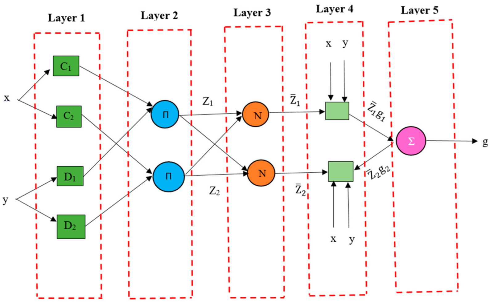
2.1. Adaptive Neuro Fuzzy Inference System (ANFIS)

The adaptive neuro fuzzy inference system (ANFIS) is a class of adaptive networks that are functionally based on Takagi-Sugeno [34] fuzzy inference systems (FIS). It is a machine learning tactic that permits the evolution of an easy-to-use model for resolving complexity. The idea behind ANFIS is to make the stated output and input variables using a set of fuzzy if-then command and appropriate membership functions (MF). The fuzzy rule established for two input (x and y) and one output (z) FIS can be given as follows:

Rule 1: If x is C₁ and y is D_1, then,

g₁ = r₁ x + s₁ y + t₁

(1)

Rule 2: If x is C₂ and y is D_2, then,

g₂ = r₂ x + s₂ y + t₂

(2)

where x and y are the two inputs, and C₁, C₂, D₁ and D₂ are membership functions (MF) linked with inputs x and y linked with the node function. The parameters r₁, s₁, t₁ and r₂, s₂, t₂ are linked with output functions g₁ and g₂, respectively. A typical ANFIS structure is shown in Figure 1, which shows that an ANFIS model contains five layers. The purpose of each of these layers is designated below:

Layer 1: Input layers are converted into a fuzzy membership function (MF) in this layer. Layer 1 parameters are designated as premise parameters. The output of the node can be reckoned as:

$$\begin{gathered} { \mathrm{O}}_{\mathrm{i}}^1={ \mathsf{\mu }}_{\mathrm{Ci}}\left(\mathrm{x}\right) \mathrm{for} \mathrm{i}=1, 2, \\ {\mathrm{O}}_{\mathrm{i}}^1={ \mathsf{\mu }}_{\mathrm{Di}-2}\left(\mathrm{y}\right) \mathrm{for} \mathrm{i}=3, 4. \end{gathered}$$

(3)

Here, x, y are the inputs to node i, and C_i and D_i are fuzzy sets in the parametric form linked with node i.

Layer 2: In this layer, nodes are fixed and act as a multiplier and are named as a neural network layer.

$${ \mathrm{O}}_{\mathrm{i}}^2={\mathrm{w}}_{\mathrm{i}}={\mathsf{\mu }}_{\mathrm{Ci}} \left(\mathrm{x}\right). {\mathsf{\mu }}_{\mathrm{Di}} \left(\mathrm{y}\right) \mathrm{for} \mathrm{i}=1, 2.$$

(4)

Layer 3: In this layer, all nodes are fixed and categorized by N. The firing strengths of fuzzy inference systems rules are normalized. Each node accessible in this layer computes the weight, which is normalized. Outputs are mentioned as normalized firing strengths.

$${ \mathrm{O}}_{\mathrm{i}}^3={\overline{\mathrm{w}}}_{\mathrm{i}}=\frac{{\mathrm{w}}_{\mathrm{i}}}{{\mathrm{w}}_1+{\mathrm{w}}_2} \mathrm{for} \mathrm{i}=1, 2.$$

(5)

Layer 4: In this layer, features of the nodes are adaptable. This is a fuzzy logic node with a parameter set {r_i, si, ti} and the output of preceding layer ${\overline{\mathrm{w}}}_{\mathrm{i}} .$The output of the node is signified below:

$${\mathrm{O}}_{\mathrm{i}}^4={\overline{\mathrm{w}}}_{\mathrm{i}}{\mathrm{g}}_{\mathrm{i}}={\overline{\mathrm{w}}}_{\mathrm{i}}\left({\mathrm{r}}_{\mathrm{i}}\mathrm{x}+{\mathrm{s}}_{\mathrm{i}}\mathrm{y}+{\mathrm{t}}_{\mathrm{i}}\right) \mathrm{for} \mathrm{i}=1, 2.$$

(6)

Layer 5: In this layer, only one node is fixed, and its output is calculated as a total of each incoming signal. The output function of this node is computed as:

$${ \mathrm{O}}_{\mathrm{i}}^5=\sum {\overline{\mathrm{w}}}_{\mathrm{i}}{\mathrm{g}}_{\mathrm{i}}=\frac{{\sum }_{\mathrm{i}}{\mathrm{w}}_{\mathrm{i}}{\mathrm{g}}_{\mathrm{i}}}{{\sum }_{\mathrm{i}}{\mathrm{w}}_{\mathrm{i}}} {\mathrm{O}}_{\mathrm{i}}^4={\overline{\mathrm{w}}}_{\mathrm{i}}{\mathrm{g}}_{\mathrm{i}}={\overline{\mathrm{w}}}_{\mathrm{i}}\left({\mathrm{r}}_{\mathrm{i}}\mathrm{x}+{\mathrm{s}}_{\mathrm{i}}\mathrm{y}+{\mathrm{t}}_{\mathrm{i}}\right) \mathrm{for} \mathrm{i}=1, 2.$$

(7)

2.2. Metaheuristic Optimization Algorithm

2.2.1. Particle Swarm Optimization (PSO)

PSO is one of the bio-inspired algorithms and is a simple one to search for an ideal solution in the space. PSO was proposed by the authors Kennedy and Eberhart in the year 1995 [35]. It practices a numeral of particles (agents) that constitute a swarm moving around in the search space, looking for the best solution. This algorithm executes the hunt of the best solution through agents, referred to as particles, whose routes are attuned by a stochastic and a deterministic component. Each particle is inclined by its ‘best’ achieved position (personnel best or pbest) and the group ‘best’ position (global best or gbest) but have a habit of moving randomly. This practice is repeated till the completion standard is reached.

2.2.2. Genetic Algorithm (GA)

GA is a kind of meta-heuristic optimization that is inspired by Charles Darwin’s theory of natural evolution [36]. GA reflects the procedure of natural selection where the suitable individuals are nominated for reproduction in order to yield offspring of the next generation. It mostly works when the idea is to transfer a population of chromosomes. GA works on three types of processes, viz. selection, crossover and mutation. The selection process chooses the entities called parents that pay to the population of the next generation. In the course of producing offspring, crossover or mutation is used. Over frequent generations, the process determines the best group of chromosomes, which should replicate the best or near-best solution to the problem. This optimization is unique as it governs the best solution to any problem.

2.2.3. Firefly Algorithm (FFA)

This is another meta-heuristic optimization proposed by the author Xin-She Yang [37]. FFA is based on flashing patterns and the behavior of fireflies. This algorithm is used to find the global bests of objective functions based on swarm intelligence, inspecting the searching performance of fireflies. Light variation and appealing formulas are the two important key components of FFA. To ascertain mates for mating, to trace prey and to raise awareness or fear among the swarm, fireflies use these lights.

2.2.4. Grey Wolf Optimization (GWO)

GWO is another meta-heuristic optimization inspired by grey wolves. Mirjalili et al. [38] proposed the grey wolf optimization inspired by the social life of a grey wolf pack. The main aim of GWO is to replicate the activity of grey wolves in nature to hunt in a cooperative way. Alpha wolf, beta wolf, delta wolf and omega wolf are the four different kinds of grey wolves that simulate the headship hierarchy. In addition, the three core phases of hunting, probing for prey, enclosing prey and attacking prey, are executed.

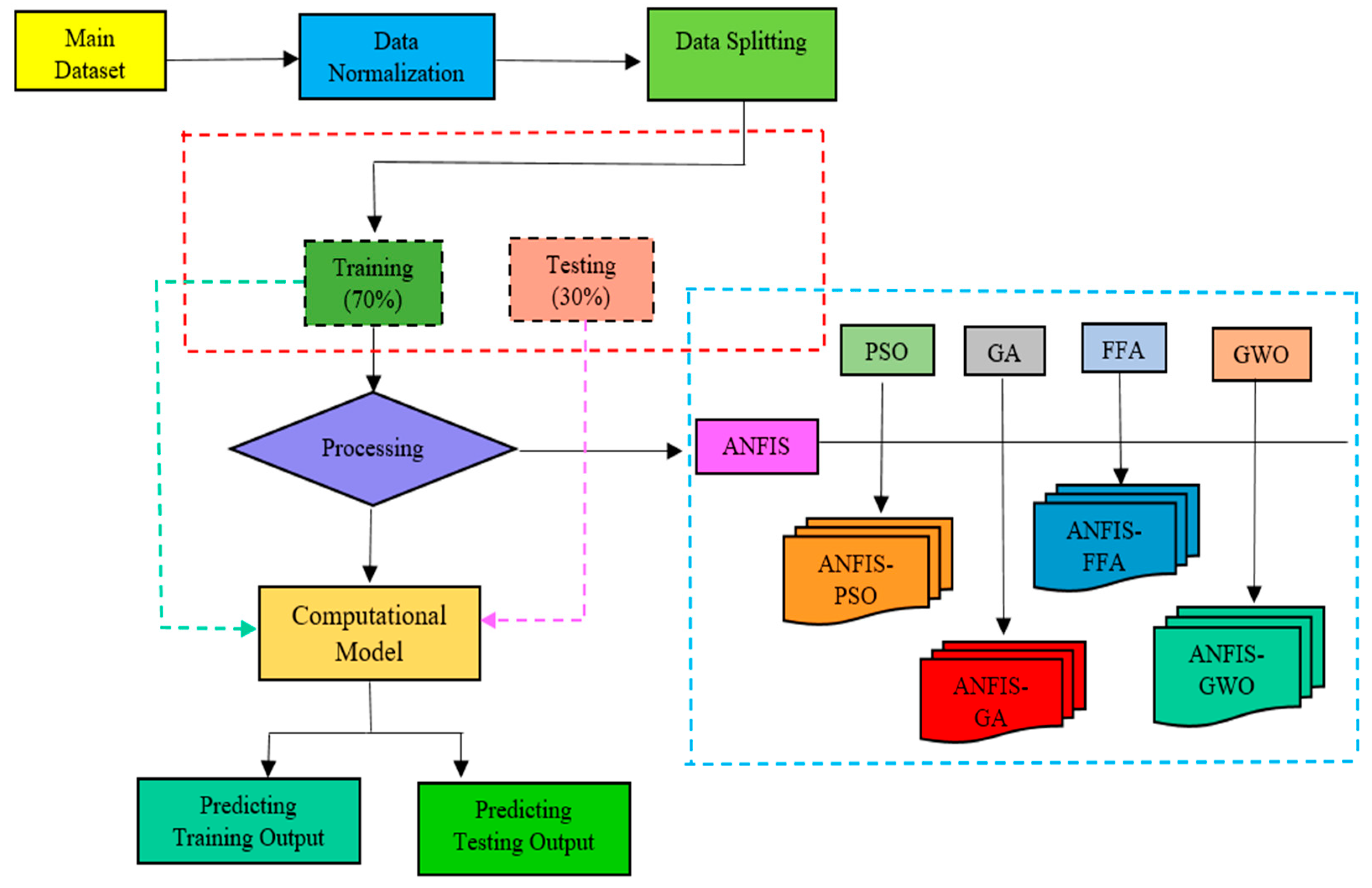
2.3. Hybrid ANFIS Models

The above-mentioned sections have emphasized the importance of the machine learning approach which advocates the necessity and presentation of these practices for judging the factor of safety against the overturning of the wall. However, the effectiveness of these methods can be debated due to the numerous restrictions and shortcomings related to them. So, scholars have established certain approaches that can be suitably accepted for improving their performance. The aforesaid method is the hybridization of these machine learning approaches along with metaheuristic optimization techniques. These meta-heuristic optimization techniques are supreme tools for solving difficult technical problems such as signaling, manufacturing, designing, data processing and many more. When these self-efficient meta-heuristic optimization techniques are pooled with a machine learning technique, the computational intelligence of these meta-heuristic optimization techniques is enriched up to a substantial level, assisting them in attaining perfect predictive validity. Because of the substantial relevancy of this idea and seeing the difficulties involved for the deciding factor of safety against overturning, the authors have implemented the same for the present study. In the present study, the association of the ANFIS model with the meta-heuristic optimization techniques selected (PSO, GA, FFA and GWO) can form the resulting hybrid models; ANFIS-PSO, ANFIS-GA, ANFIS-FFA and ANFIS-GWO, respectively. The various advantages using PSO with ANFIS are that it can be easily parallelized for concurrent processing, there are less algorithm parameters and it has an efficient global search algorithm. However, it also has some drawbacks, for example, its optimum local search ability is poor. The major advantages of using FFA are that it can efficiently deal with non-linear, multi-modal optimization and the convergence speed is very high while finding a global optimized response. High computational time complication is the drawback of PSO. The advantage of GA is that it supports multi-objective function, and it uses a probabilistic transition rule instead of deterministic rules, but it is computationally expensive and needs less information about the problem. As we know that PSO and GWO are swarm intelligence-based algorithms, the major advantage of GWO is also like PSO in that it has less algorithm parameters and magnificent potential in solving the problems but it has poor local searching capability and a slow convergence rate.

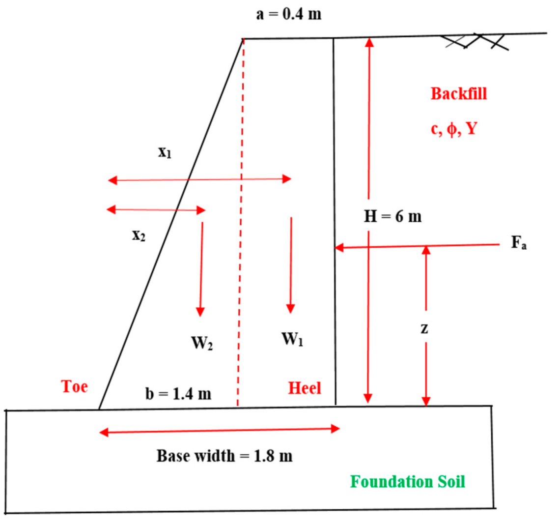
3. Practical Applications to the Gravity Retaining Wall

A gravity retaining wall mainly depends on their bulky weight to hold the material at the back of it and attain stability against numerous modes of failures. A gravity retaining wall is employed to inspect probabilistic analysis. The overturning failure mode is inspected by various hybrid ANFIS models. Figure 2 illustrates the geometry of a gravity retaining wall and the various dimensions considered in the article. The factor of safety (FOS) against overturning can be designated below:

$${\mathrm{FOS}}_{\mathrm{ovt}}=\frac{\sum {\mathrm{M}}_{\mathrm{R}}}{\sum {\mathrm{M}}_{\mathrm{O}}}=\frac{{\mathrm{W}}_1.{ \mathrm{x}}_1+{ \mathrm{W}}_2.{ \mathrm{x}}_2}{{\mathrm{F}}_{\mathrm{a}}. \mathrm{z}}$$

(8)

where M_R and M_O indicate the resisting moment and overturning moment, respectively, W₁ and W₂ are the element weights of the gravity retaining wall (GRW), x₁ and x₂ are the horizontal lever distance from the toe wall, z is the vertical lever distance and Fa is the total active thrust per meter run of the wall. In this work, a classical earth pressure theory, namely Rankine’s theory, is used to compute total active force, which is established on the assumption that the there is no friction between rear of the wall and backfill. For the backfill properties with c, φ and Υ, F_a is given by

$${\mathrm{F}}_{\mathrm{a}}=\frac{1}{2} {\mathrm{k}}_{\mathrm{a}}\mathsf{\gamma }{\mathrm{H}}^2 -2\mathrm{cH}\sqrt{{\mathrm{k}}_{\mathrm{a}}}+\frac{2{\mathrm{c}}^2}{\mathsf{\gamma }}$$

(9)

Here, H is the wall height and k_a is the active earth pressure coefficient, which is the function of φ and expressed as

$${\mathrm{k}}_{\mathrm{a}}=\frac{1-\sin \mathsf{\phi }}{1+\sin \mathsf{\phi }}={\tan }^2 (\frac{\mathsf{\pi }}{4}-\frac{\mathsf{\phi }}{2})$$

(10)

In Figure 2, component weight W₁ and W₂ and lever arm distance can be computed as

$${\mathrm{W}}_1={\mathsf{\Upsilon }}_{\mathrm{wall}} \mathrm{a} \mathrm{H}; {\mathrm{W}}_2=\frac{1}{2}{ \mathsf{{\rm Y}}}_{\mathrm{wall}} \mathrm{b} \mathrm{H}; {\mathrm{x}}_1=\mathrm{b}+\frac{\mathrm{a}}{2} ; {\mathrm{x}}_2=\frac{2}{3}\mathrm{b}; \mathrm{z}=\mathrm{H}/3$$

(11)

As shown in Figure 2, cohesion (c), angle of shearing resistance (φ) and unit weight of backfill (ϒ) have a significant influence on the computation of factor of safety against overturning failure.

This research has much to contribute both to the field of artificial intelligence (AI) and geotechnical engineering. Statistical input parameters are taken as cohesion (c), angle of shearing resistance (φ) and unit weight of soil (Υ), which follows normal distribution function. Other parameters such as H, a, b and ϒ_wall are supposed to be constant so that correlation between c, φ and ϒ can be efficiently explored without intervention from other random variables. For this learning of gravity retaining walls, data were generated and the coefficient of variation (CoV) values were taken from different previous studies [5,39], and statistical depictions of the dataset are mentioned in

Table 1. Statistical depiction of dataset.

Parameters	Cohesion (c)	Unit Weight of Soil (ϒ)	Angle of Shearing Resistance (φ)
Mean	11 kN/m2	16 kN/m3	290
Coefficient of variation (%)	20	6	12
Standard deviation	2.2	0.96	3.48
Minimum	5.64 kN/m2	13.49 kN/m3	21.140
Maximum	16.93 kN/m2	17.84 kN/m3	37.520
Median	11.53	15.98	28.72
Range	11.29	4.34	16.39
Standard Error	0.22	0.096	0.35
Sample Variance	5.85	0.96	11.49
Kurtosis	−0.138	−0.455	−0.105
Skewness	−0.097	−0.019	0.286

.

A correlation plot is drawn for input variables (c, ϒ and φ) and the response variable (FOS) as shown in Figure 3. It is observed from the correlation plot that the input variables (c, ϒ and φ) are highly correlated amongst themselves which improves the difficulty of multicollinearity in the training and testing of computational models. Pearson’s correlation coefficient (R) indicates that there is a linear correlation between two variables and describes the strength of the link between the two variables. The collinearity among cohesion of soil (c) and factor of safety (FOS) was the strongest (c, R = 0.70). Additionally, input parameters such as unit weight of soil (ϒ, R = −0.29) and angle of shearing resistance (φ, R = 0.59) have a substantial extent of correlation to the FOS against overturning. A scatter plot is also drawn in Figure 4 to envisage the correlation among any two sets of data (c vs. FOS, ϒ vs. FOS and φ vs. FOS).

Before the evolution of the machine learning model, the normalization of datasets is one of the key stages. Normalization is performed to remove the dimensionality influence of the variables. Therefore, before generating any model in the present study, the input and output variables were normalized between 0 and 1 using the formulation, as follows:

$${\mathrm{Z}}_{\mathrm{Normalised}}=(\frac{\mathrm{Z}-{\mathrm{Z}}_{\min }}{{\mathrm{Z}}_{\max }-{\mathrm{Z}}_{\min }})$$

(12)

Here, Z_min and Z_max are the minimum and maximum values of the parameter (Z) under consideration, respectively.

After the normalization has been performed, the dataset is then divided into training and testing phases. For this, 70% of the entire dataset is removed to form the training phase, and the remaining 30% of the dataset is used as the testing phase.

ANFIS-PSO, ANFIS-GA, ANFIS-FFA and ANFIS-GWO hybrid models were used to forecast the factor of safety against overturning. Numerous assessments were performed to observe the performance of these models.

4. Statistical Performance Parameters

The prediction accuracy of Hybrid ANFIS models such as ANFIS-PSO, ANFIS-GA, ANFIS-FFA and ANFIS-GWO were examined using various statistical performance parameters and through graphical appraisal (i.e., scatter plot, R-curve, Williams plot and accuracy matrix). Various statistical performance parameters were used such as coefficient of determination (R²), root mean square error (RMSE), variance account factor (VAF), Willmott’s index of agreement (WI), Legate and McCabe’s index (LMI), scatter index (SI), a-20 index, performance index (PI), Kling Gupta efficiency (KGE), normalized mean bias error (NMBE), mean absolute error (MAE) and mean bias error (MBE).

$${\mathrm{R}}^2=\frac{{\sum }_{\mathrm{i}=1}^{\mathrm{n}}{({\mathrm{F}}_{\mathrm{obs},\mathrm{i}}-{\overline{\mathrm{F}}}_{\mathrm{obs}})}^2-{\sum }_{\mathrm{i}=1}^{\mathrm{n}}{({\mathrm{F}}_{\mathrm{obs},\mathrm{i}}-{\mathrm{F}}_{\mathrm{pre},\mathrm{i}})}^2}{{\sum }_{\mathrm{i}=1}^{\mathrm{n}}{({\mathrm{F}}_{\mathrm{obs},\mathrm{i}}-{\overline{\mathrm{F}}}_{\mathrm{obs}})}^2}$$

(13)

$$\mathrm{RMSE}=\sqrt{\frac{1}{\mathrm{n}}} {\sum }_{\mathrm{i}=1}^{\mathrm{n}}{\left({\mathrm{F}}_{\mathrm{obs},\mathrm{i}}-{\mathrm{F}}_{\mathrm{pre},\mathrm{i}}\right)}^2$$

(14)

$$\mathrm{VAF}=(1- \frac{\mathrm{var}\left({\mathrm{F}}_{\mathrm{obs},\mathrm{i}}-{\mathrm{F}}_{\mathrm{pre},\mathrm{i}}\right)}{\mathrm{var}\left({\mathrm{F}}_{\mathrm{obs},\mathrm{i}}\right)})\times 100$$

(15)

$$\mathrm{WI}=1-[\frac{{\sum }_{\mathrm{i}=1}^{\mathrm{n}}{({\mathrm{F}}_{\mathrm{obs},\mathrm{i}}-{\mathrm{F}}_{\mathrm{pre},\mathrm{i}})}^2}{{\sum }_{\mathrm{i}=1}^{\mathrm{n}}{\left(\left|{\mathrm{F}}_{\mathrm{pre},\mathrm{i}}-{\overline{\mathrm{F}}}_{\mathrm{obs}}\right|+\left|{\mathrm{F}}_{\mathrm{obs},\mathrm{i}}-{\overline{\mathrm{F}}}_{\mathrm{obs}}\right|\right)}^2}]$$

(16)

$$\mathrm{LMI}=1-[ \frac{{\sum }_{\mathrm{i}=1}^{\mathrm{n}}\left|{\mathrm{F}}_{\mathrm{obs},\mathrm{i}}-{\mathrm{F}}_{\mathrm{pre},\mathrm{i}} \right|}{{\sum }_{\mathrm{i}=1}^{\mathrm{n}}\left|{\mathrm{F}}_{\mathrm{obs},\mathrm{i}}-{\overline{\mathrm{F}}}_{\mathrm{obs}}\right|} ]$$

(17)

$$\mathrm{SI}= \frac{\sqrt{\frac{1}{\mathrm{n}} {\sum }_{\mathrm{i}=1}^{\mathrm{n}}{\left({\mathrm{F}}_{\mathrm{obs},\mathrm{i}}-{\mathrm{F}}_{\mathrm{pre},\mathrm{i}}\right)}^2}}{{\overline{\mathrm{F}}}_{\mathrm{obs}}}= \frac{\mathrm{RMSE}}{{\overline{\mathrm{F}}}_{\mathrm{obs}}}$$

(18)

$$\mathrm{a}-20 \mathrm{Index}=\frac{\mathrm{m}20}{\mathrm{n}}$$

(19)

PI = AdjR² + 0.01VAF − RMSE

(20)

$${\mathrm{AdjR}}^2=1-\frac{\left(\mathrm{n}-1\right)}{\left(\mathrm{n}-\mathrm{m}-1\right)}\left(1-{\mathrm{R}}^2\right)$$

(21)

$$\mathrm{KGE}=1-\sqrt{{\left({\mathrm{R}}^2-1\right)}^2+{(\frac{{\overline{\mathrm{F}}}_{\mathrm{pre}}}{{\overline{\mathrm{F}}}_{\mathrm{obs}}}-1)}^2+{(\frac{{\mathrm{CoV}}_{\mathrm{pre}}}{{\mathrm{CoV}}_{\mathrm{obs}}}-1)}^2}$$

(22)

$$\mathrm{NMBE}=\frac{\frac{1}{\mathrm{n}} {\sum }_{\mathrm{i}=1}^{\mathrm{n}}\left({\mathrm{F}}_{\mathrm{pre},\mathrm{i}}-{\mathrm{F}}_{\mathrm{obs},\mathrm{i}}\right)}{\frac{1}{\mathrm{n}}{\sum }_{\mathrm{i}=1}^{\mathrm{n}}{\mathrm{F}}_{\mathrm{obs},\mathrm{i}}} \times 100$$

(23)

$$\mathrm{MAE}=\frac{1}{\mathrm{n}} {\sum }_{\mathrm{i}=1}^{\mathrm{n}}\left|\left({\mathrm{F}}_{\mathrm{pre},\mathrm{i}}-{\mathrm{F}}_{\mathrm{obs},\mathrm{i}}\right)\right|$$

(24)

$$\mathrm{MBE}=\frac{1}{\mathrm{n}} {\sum }_{\mathrm{i}=1}^{\mathrm{n}}\left({\mathrm{F}}_{\mathrm{pre},\mathrm{i}}-{\mathrm{F}}_{\mathrm{obs},\mathrm{i}} \right)$$

(25)

Here, F_obs,i and F_pre,i are the actual and predicted ith value, respectively, ${\overline{\mathrm{F}}}_{\mathrm{obs}}$ and ${\overline{\mathrm{F}}}_{\mathrm{pre}}$ are the mean of actual and predicted value, respectively, n is the number of training or testing samples, m is the model input capacity, m20 is the amount of data with observed/predicted value ratio between 0.80 and 1.20. By using Equations (13)–(25), the model has a minimum value of RMSE, NMBE, MBE, MAE and SI and a higher value of R², AdjR², VAF, PI, WI, LMI, KGE, a-20 Index and NS indicates better prediction power of the model.

5. Methodology Flowchart

The methodology of the existing learning can be systematized in the following stages (Figure 5).

Stage 1: In this stage, the main dataset is generated, and after this, the normalization of the dataset is performed.

Stage 2: In this stage, normalized data (100 dataset) are split into two parts, namely training (70%) and testing (30%) datasets.

Stage 3: In this stage, data are processed, and learning and validation is performed. Four AI models, namely ANFIS-PSO, ANFIS-GA, ANFIS-FFA and ANFIS-GWO, were trained using the training dataset. Statistical performance parameters were used to validate the model.

Stage 4: In this stage, the output (FOS) is predicted for the training (TR) and testing (TS) datasets.

6. Results and Analysis

6.1. Prediction Command

In this section, the factor of safety (FOS) against overturning was predicted using four machine learning models, namely ANFIS-PSO, ANFIS-GA, ANFIS-FFA and ANFIS-GWO. The capability of these models was judged by computing the statistical parameters, namely R², AdjR², RMSE, VAF, WI, LMI, SI, a-20 Index, PI, KGE, NMBE, MAE and MBE. The results of the evaluation statistics for the training (TR) and testing (TS) phases are provided in

Table 2. Comparison of model prediction power (training dataset).

Parameters	Ideal Value	ANFIS-GA (Training)	ANFIS-PSO (Training)	ANFIS-FFA (Training)	ANFIS-GWO (Training)
R2	1	0.984	0.997	0.995	0.897
AdjR2	1	0.983	0.996	0.995	0.893
RMSE	0	0.025	0.012	0.014	0.063
VAF	100	98.594	99.617	99.510	89.836
WI	1	0.996	0.999	0.998	0.968
LMI	1	0.882	0.939	0.933	0.724
SI	0.1	0.096	0.047	0.054	0.244
a-20 Index	1	0.841	0.886	0.913	0.786
PI	2	1.944	1.981	1.976	1.728
KGE	1	0.936	0.994	0.922	0.762
NMBE	0	3.347	0.144	0.590	2.4062
MAE	0	0.0182	0.009	0.011	0.042
MBE	0	0.009	0.001	0.002	0.006

and

Table 3. Comparison of model prediction power (testing dataset).

Parameters	Ideal Value	ANFIS-GA (Testing)	ANFIS-PSO (Testing)	ANFIS-FFA (Testing)	ANFIS-GWO (Testing)
R2	1	0.953	0.966	0.989	0.842
AdjR2	1	0.948	0.963	0.988	0.824
RMSE	0	0.048	0.040	0.023	0.087
VAF	100	95.351	96.655	99.005	84.190
WI	1	0.987	0.991	0.997	0.945
LMI	1	0.784	0.842	0.900	0.656
SI	0.1	0.201	0.169	0.095	0.368
a-20 Index	1	0.767	0.733	0.867	0.767
PI	2	1.853	1.889	1.955	1.579
KGE	1	0.913	0.928	0.930	0.664
NMBE	0	2.265	1.374	2.401	1.279
MAE	0	0.031	0.023	0.014	0.050
MBE	0	0.005	0.003	0.006	0.003

. A comparison of four hybrid models was performed based on statistical indices. Based on the outcome, it has been observed that ANFIS-PSO has achieved better prediction power with a higher value of R² = 0.997, VAF = 99.617, WI = 0.999, LMI = 0.939, PI = 1.981 and KGE = 0.994, and a lower value of RMSE = 0.012, SI = 0.047, NMBE = 0.144, MAE = 0.009 and MBE = 0.001 in the training phase, while the same is decreased in the testing phase (R² = 0.966, VAF = 96.655, WI = 0.991, LMI = 0.842, PI = 1.889, KGE = 0.928, RMSE = 0.04, SI = 0.169, NMBE = 1.734, MAE = 0.023 and MBE = 0.003). The performance of the ANFIS-FFA model (R² = 0.995, VAF = 99.51, WI = 0.998, LMI = 0.933, PI = 1.976, KGE = 0.922, RMSE = 0.014, SI = 0.054, NMBE = 0.590, MAE = 0.011 and MBE = 0.002) in the training phase is found to be marginally lower than the ANFIS-PSO model, while a higher predicting power (R² = 0.989, VAF = 99.005, WI = 0.997, LMI = 0.900, PI = 1.955, KGE = 0.930, RMSE = 0.023, SI = 0.095, NMBE = 2.401, MAE = 0.014 and MBE = 0.006) is perceived in the testing part as compared to the ANFIS-PSO model. Overall, we can say that, out of the four hybrid ANFIS models, the ANFIS-PSO model has better predictive power in the training phase and ANFIS-FFA in the testing phase.

6.2. Rank Analysis

In this section, rank analysis is performed, as shown in

Table 4. Rank analysis of hybrid ANFIS model (training and testing dataset).

Hybrid Models	Phase	R2	RMSE	VAF	WI	LMI	SI	a-20 Index	PI	KGE	NMBE	MAE	MBE	Total Rank	Overall Rank
ANFIS-GA	TR	2	3	3	3	3	3	3	3	2	4	3	4	36	70
	TS	3	3	3	3	3	3	2	3	3	3	3	2	34
ANFIS-PSO	TR	1	1	1	1	1	1	2	1	1	1	1	1	13	37
	TS	2	2	2	2	2	2	3	2	2	2	2	1	24
ANFIS-FFA	TR	3	2	2	2	2	2	1	2	3	2	2	2	25	42
	TS	1	1	1	1	1	1	1	1	1	4	1	3	17
ANFIS-GWO	TR	4	4	4	4	4	4	4	4	4	3	4	3	46	86
	TS	4	4	4	4	4	4	2	4	4	1	4	1	40

. After calculating all the statistical indices for the training (TR) and testing (TS) phases, models are ranked consequently. The model value that indicates the best performance is ranked 1, and the model with the worst performance is ranked 4 (as four models are used in this study). Afterward, all the ranks are added to get an overall rank, which is also computed in this learning. The model that has the lowermost rank is treated as the best performing model, and the highest rank indicated the lowest performing model. From Table 4, it is observed that the total ranks and overall ranks are as follows: ANFIS-PSO—Rank_TR = 13, Rank_TS = 24 and overall rank = 37; ANFIS-FFA—Rank_TR = 25, Rank_TS = 17 and overall rank = 42; ANFIS-GA—Rank_TR = 36, Rank_TS = 34 and overall rank = 70; and ANFIS-GWO—Rank_TR = 46, Rank_TS = 40 and overall rank = 86. This provides a complete assessment of the prediction power and presentation of the model. Therefore, the ANFIS-PSO has a very good performance out of all four developed models for predicting FOS against overturning.

6.3. Reliability Analysis

Safety factor concept cannot be directly considered as a reliable output for risk evaluation as a prominent number of uncertainties may be involved. This error can be linked with the backfill properties or analytical method used. Reliability analysis has been carried out to justify uncertainties and to obtain a reliable approach for predicting the factor of safety against overturning. The first-order second moment (FOSM) approach is applied to compute the reliability index (β). In the FOSM method, µ_z and σ_z are the mean value and the standard deviations of the performance function X, respectively. Resisting moment (M_R) and overturning moment (M_O) are represented as R and S, respectively, and ${\mathsf{\mu }}_{\mathrm{R}}$ and ${\mathsf{\mu }}_{\mathrm{S}}$ are the mean values and ${\mathsf{\sigma }}_{\mathrm{R}}$ and ${\mathsf{\sigma }}_{\mathrm{S}}$ are the standard deviations of R and S, respectively.

$$\mathsf{\beta }=\frac{{\mathsf{\mu }}_{\mathrm{X}}}{{\mathsf{\sigma }}_{\mathrm{X}}}=\frac{{\mu }_{\mathrm{R}}-{\mu }_{\mathrm{S}}}{\sqrt{{\mathsf{\sigma }}_{\mathrm{R}}{}^2+{\mathsf{\sigma }}_{\mathrm{S}}{}^2}}$$

(26)

Overturning probability relies significantly on mean and variance of obtained factor of safety; therefore, the reliability index in terms of factor of safety (F) is obtained as:

$$\mathsf{\beta }=\frac{{\mu }_{\mathrm{F}}-1}{{\mathsf{\sigma }}_{\mathrm{F}}}$$

(27)

where ${\mu }_{\mathrm{F}}$ and ${\mathsf{\sigma }}_{\mathrm{F}}$ are the mean and standard deviation of factor of safety, respectively. The probability of failure (P_f) is directly related to the reliability index (β) by assuming that all the normal variables are normally distributed. The probability of failure can be computed as:

P_f = 1 − φ (β)

(28)

where φ (β) is the standard normal cumulative probability. The reliability index (β) of the model is computed using first-order second moment method (FOSM) and compared with the actual value of the reliability index. A higher value of β indicates a greater performance of the model.

Table 5. Comparison of different models on the basis of reliability index (β).

Models	Actual β	Actual Pf	Model’s β	Model’s Pf	Rank
ANFIS-GA	1.421	0.078	1.273	0.102	3
ANFIS-PSO			1.324	0.092	1
ANFIS-FFA			1.320	0.093	2
ANFIS-GWO			1.256	0.105	4

shows that the performance of ANFIS-PSO is the best out of all four models due to the higher value of the reliability index and lower value of the probability of failure (P_f). On the basis of β and P_f, models are ranked accordingly. The better performing model (higher β and lower value of P_f) is ranked 1, and the worst performing model (lower β and higher value of P_f) is ranked 4.

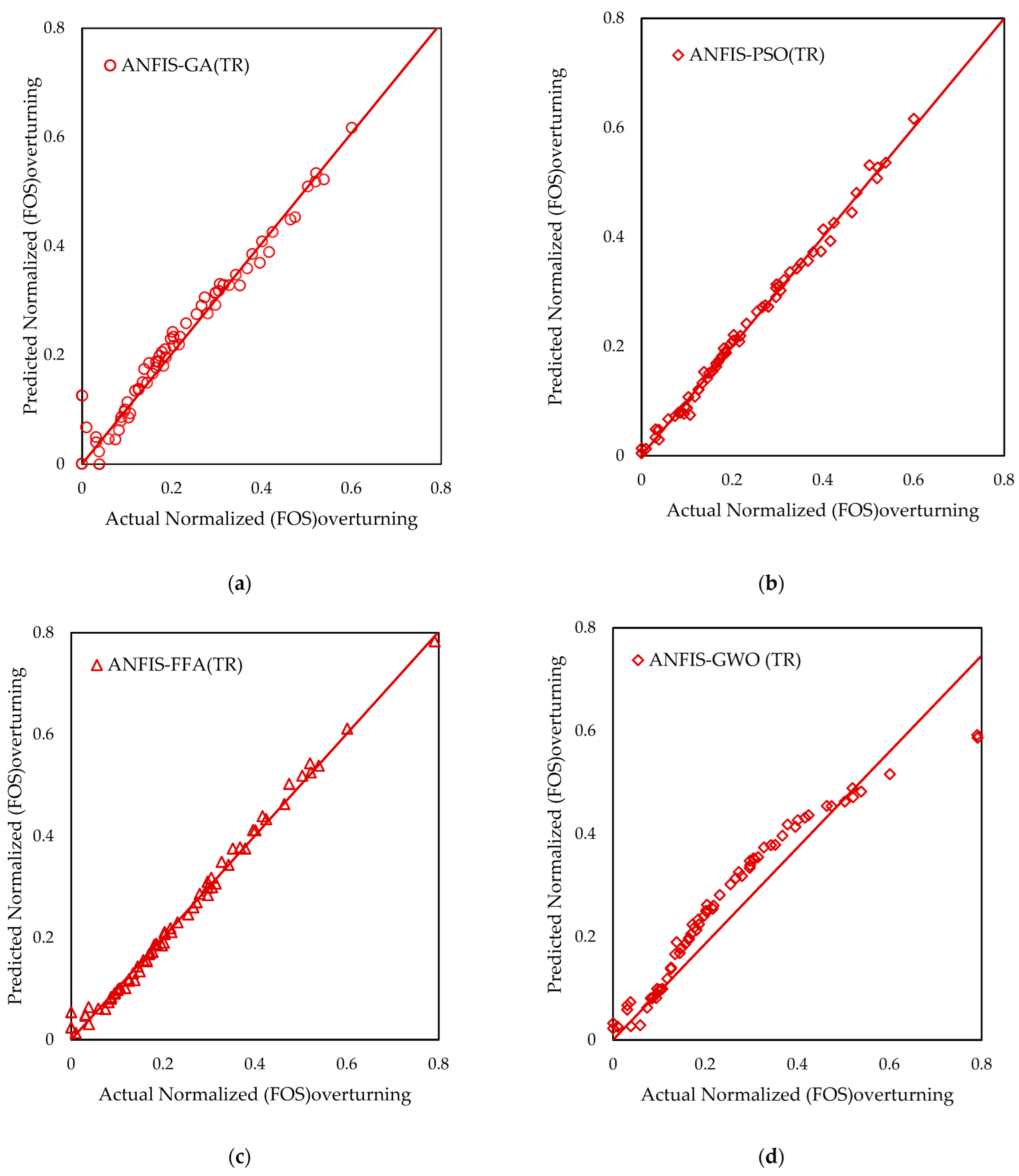
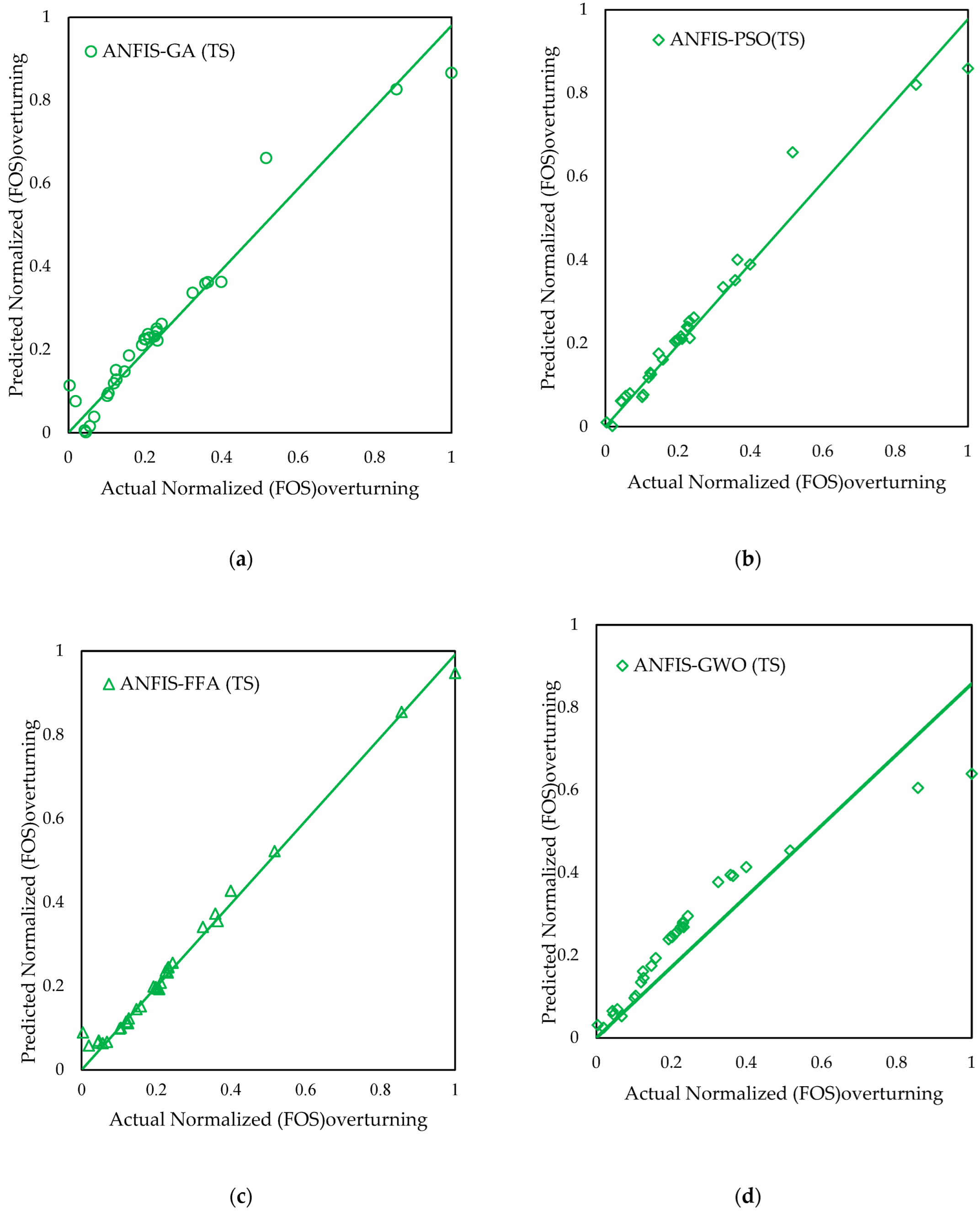
6.4. Regression Curve

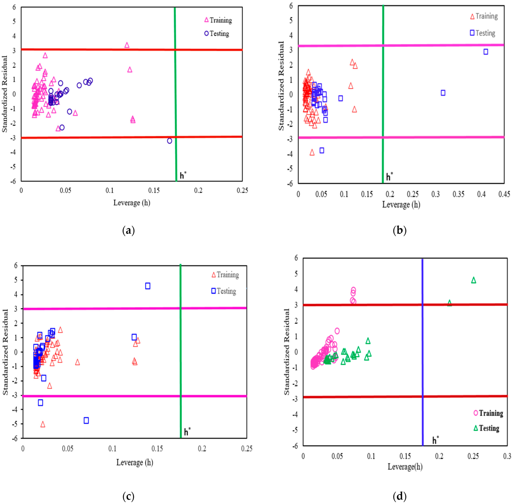
The regression or performance curve is the plot between the actual and predicted value of FOS. It indicates whether the model tracks the reference models. This curve provides an R-value calculated and indicated in the table (Table 2 and Table 3).

Figure 6 and Figure 7 is the plot between the observed FOS (Normalized) and predicted FOS (Normalized) against overturning using the training and testing datasets. From the above plot, it is perceived that the models ANFIS-PSO and ANFIS-FFA overlap each other and follow almost the same style. Minor deviations can be witnessed in the model ANFIS-GA, and significant deviance is observed in ANFIS-GWO for the training and testing datasets. From the other measures, it has been realized that, as compared to the ANFIS-PSO and ANFIS-FFA models, the ANFIS-GA and ANFIS-GWO models have slightly reduced prediction ability.

6.5. Williams Plot

The valuation of the applicability domain of four different AI models is considered a vital stage in deciding whether the model is reliable in making predictions. Applicability domains were recognized for four different AI models by describing the leverage (h) values for both training (TR) and testing (TS) datasets. Figure 8 specifies the Williams plot—a graphical representation of standardized residual on the ordinate and leverages (h) on the abscissa for each compound of the training and testing datasets. From these plots, the applicability domain is enclosed inside a squared zone within $\pm 3$ standard deviations and a leverage threshold h* (h* = 3 p/k, where k is the number of training compounds and p is the number of model parameters plus one). The trial compound with leverages h < h* are reflected to be reliably predicted by the model.

The Williams plot for the training and testing datasets shown in Figure 8a–d finds the applicability domain of the hybrid ANFIS model within standardized residual ($\pm 3 \mathsf{\sigma })$ and a leverage threshold h* = 0.172. From Figure 8a–d, it has been observed that all the compounds of the training and testing dataset have leverage (h) less than h*, but one training and one testing compound lies outside the squared zone ($\pm 3 \mathsf{\sigma })$ for the ANFIS-PSO model, for ANFIS-FFA model one training and one testing compound have leverage (h) less than h* but outside the squared zone ($\pm 3 \mathsf{\sigma })$ and two testing compound have leverage (h) exceeding the leverage threshold (h*), but inside the squared zone ($\pm 3 \mathsf{\sigma })$ for the ANFIS-GA model, all training and testing compounds have leverages less than the leverage threshold, but one training and three testing compounds lie outside the established zone ($\pm 3 \mathsf{\sigma })$, and for the ANFIS-GWO model, all training and testing compounds have h < h* except two testing compounds which have h > h* and also outside the squared zone, and four training compounds have h < h* but are outside the established zone. The above observations from the Williams plot indicates that they are not to be considered outliers but significant compounds.

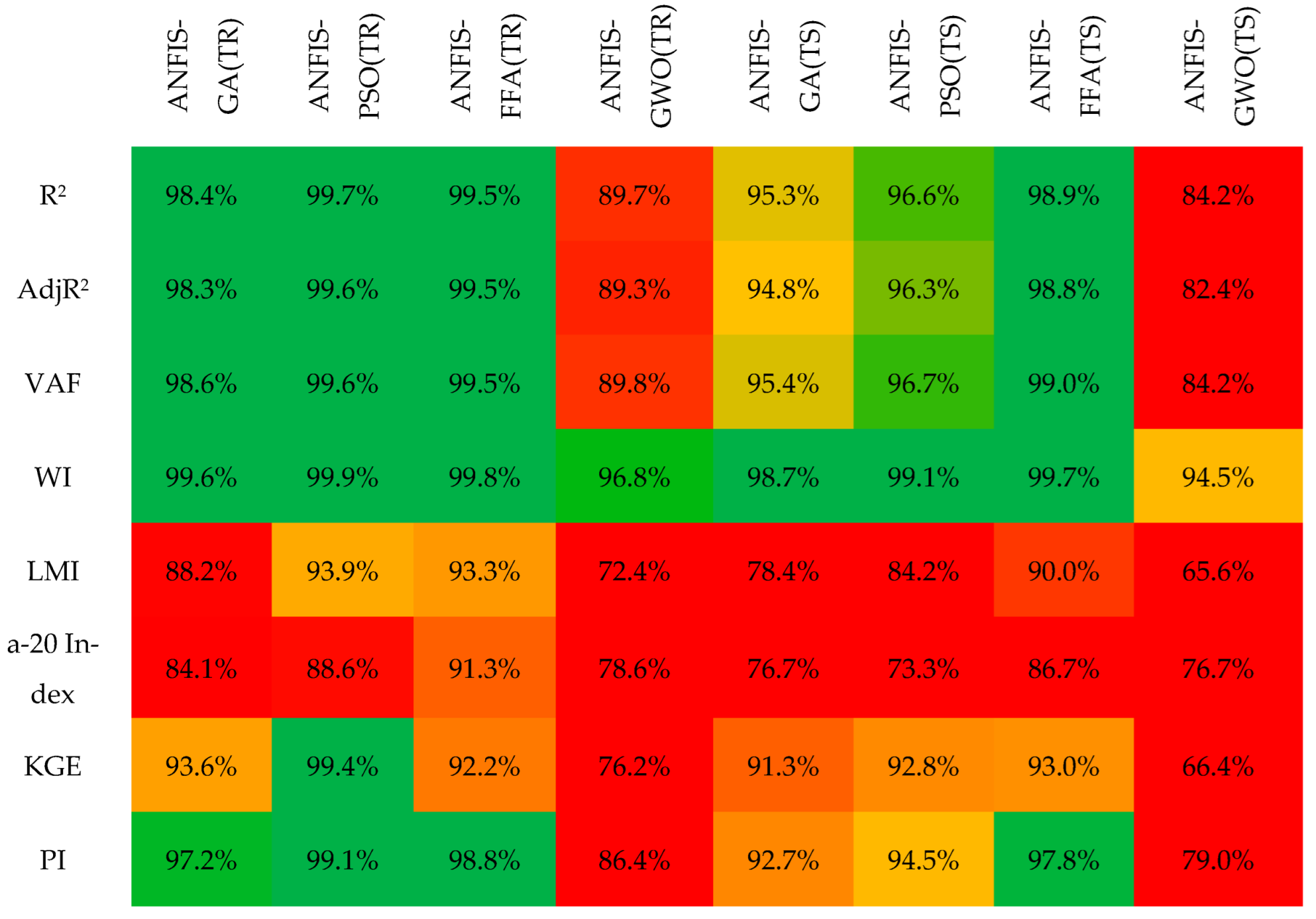
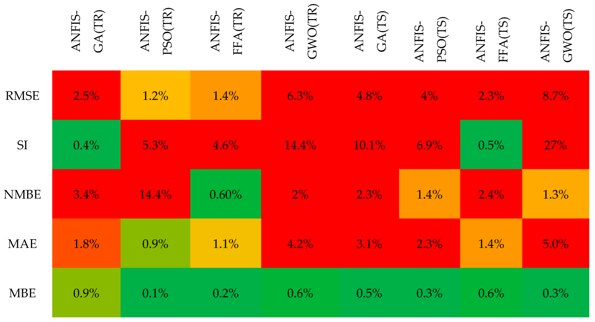
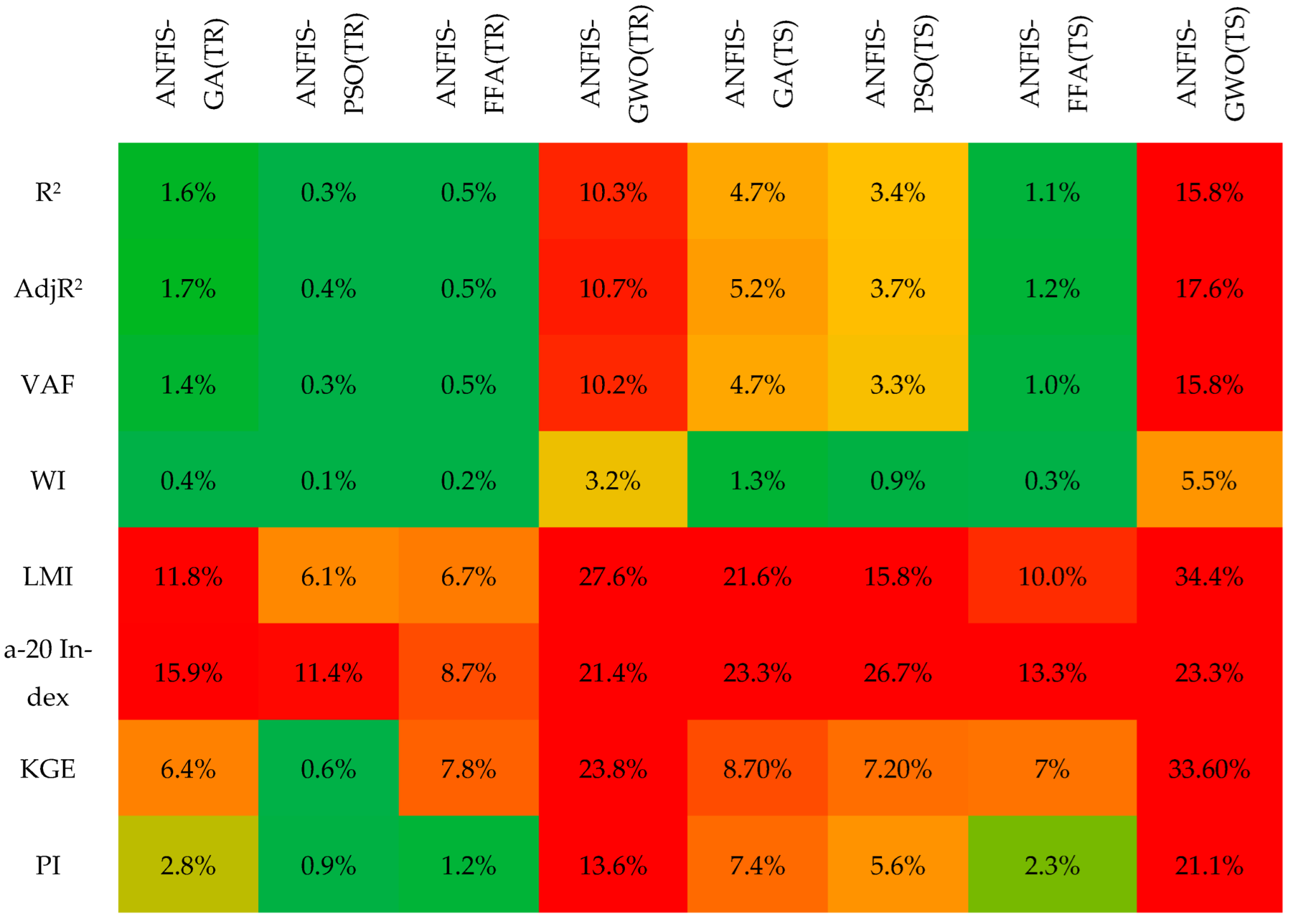
6.6. Accuracy and Error Matrix

An error matrix is a table that allows us to imagine the presentation of a hybrid ANFIS by relating the predicted value of the target variable with its ideal value. It evaluates and offers a graphic depiction of the quantity of error of the predictive models and is assessed contrary to the ideal values of each performance parameter. It also gives the idea of extreme and least values of error of a predictive model. So, the extent of error (ε %) of a predictive model can be computed using the two terms given below for error measuring parameters (RMSE, SI, NMBE, MAE and MBE) and trend measuring parameters (R², AdjR², VAF, WI, a-20 Index, KGE and PI), respectively.

ε_e = |(I_e − |P_e|)| × 100

(29)

$${\mathsf{\epsilon }}_{\mathrm{t}}=\frac{\left({\mathrm{I}}_{\mathrm{r}}-\left|{\mathrm{P}}_{\mathrm{r}}\right|\right)}{{\mathrm{I}}_{\mathrm{r}}} \times 100$$

(30)

where ε_t and ε_e represent the error for trend measuring parameters and error for error measuring parameters, respectively; I_e and I_r are the ideal values for error measuring and trend measuring parameters, respectively; P_e and P_r are the performance indices estimated for error measuring and trend measuring parameters, respectively. Using Equations (29) and (30), error is computed based on different measuring parameters (error measuring and trend measuring parameters), which are indicated in

Table 6. Computed error for error measuring parameters (training dataset).

Error Measuring Parameters	Ideal Value	ANFIS-GA (TR)	Error (εe)	ANFIS-PSO (TR)	Error (εe)	ANFIS-FFA (TR)	Error (εe)	ANFIS-GWO (TR)	Error (εe)
RMSE	0	0.025	2.5%	0.012	1.2%	0.014	1.4%	0.063	6.3%
SI	0.1	0.096	0.4%	0.047	5.3%	0.054	4.6%	0.244	14.4%
NMBE	0	3.347	3.4%	0.144	14.4%	0.590	0.6%	2.4062	2.4%
MAE	0	0.0182	1.8%	0.009	0.9%	0.011	1.1%	0.042	4.2%
MBE	0	0.009	0.9%	0.001	0.1%	0.002	0.2%	0.006	0.6%

,

Table 7. Computed error for error measuring parameters (testing dataset).

Error Measuring Parameters	Ideal Value	ANFIS-GA (TS)	Error (εe)	ANFIS-PSO (TS)	Error (εe)	ANFIS-FFA (TS)	Error (εe)	ANFIS-GWO (TS)	Error (εe)
RMSE	0	0.048	4.8%	0.040	4%	0.023	2.3%	0.087	8.7%
SI	0.1	0.201	10.1%	0.169	6.9%	0.095	0.5%	0.368	26.8%
NMBE	0	2.265	2.3%	1.374	1.4%	2.401	2.4%	1.279	1.3%
MAE	0	0.031	3.1%	0.023	2.3%	0.014	1.4%	0.050	5%
MBE	0	0.005	0.5%	0.003	0.3%	0.006	0.6%	0.003	0.3%

,

Table 8. Computed error for trend measuring parameters (training dataset).

Trend Measuring Parameters	Ideal Value	ANFIS-GA (TR)	Error (εt)	ANFIS-PSO (TR)	Error (εt)	ANFIS-FFA (TR)	Error (εt)	ANFIS-GWO (TR)	Error (εt)
R2	1	0.984	1.6%	0.997	0.3%	0.995	0.5%	0.897	10.3%
AdjR2	1	0.983	1.7%	0.996	0.4%	0.995	0.5%	0.893	10.7%
VAF	100	98.594	1.4%	99.617	0.3%	99.510	0.5%	89.836	10.2%
WI	1	0.996	0.4%	0.999	0.1%	0.998	0.2%	0.968	3.2%
LMI	1	0.882	11.8%	0.939	6.1%	0.933	6.7%	0.724	27.6%
a-20 Index	1	0.841	15.9%	0.886	11.4%	0.913	8.7%	0.786	21.4%
KGE	1	0.936	6.4%	0.994	0.6%	0.922	7.8%	0.762	23.8%
PI	2	1.944	2.8%	1.981	0.9%	1.976	1.2%	1.728	13.6%

and

Table 9. Computed error for trend measuring parameters (testing dataset).

Trend Measuring Parameters	Ideal Value	ANFIS-GA (TS)	Error (εt)	ANFIS-PSO (TS)	Error (εt)	ANFIS-FFA (TS)	Error (εt)	ANFIS-GWO (TS)	Error (εt)
R2	1	0.953	4.7%	0.966	3.4%	0.989	1.1%	0.842	15.8%
AdjR2	1	0.948	5.2%	0.963	3.7%	0.988	1.2%	0.824	17.6%
VAF	100	95.351	4.7%	96.655	3.3%	99.005	1.0%	84.190	15.8%
WI	1	0.987	1.3%	0.991	0.9%	0.997	0.3%	0.945	5.5%
LMI	1	0.784	21.6%	0.842	15.8%	0.900	10%	0.656	34.4%
a-20 Index	1	0.767	23.3%	0.733	26.7%	0.867	13.3%	0.767	23.3%
KGE	1	0.913	8.7%	0.928	7.2%	0.930	7.0%	0.664	33.6%
PI	2	1.853	7.4%	1.889	5.6%	1.955	2.3%	1.579	21.1%

.

Figure 9 indicates the accuracy matrix of the developed hybrid models for both training and testing dataset. From the accuracy matrix plot, we can see that ANFIS-PSO has higher accuracy as compared to other three model for the training dataset but the difference is minimal in case of ANFIS-PSO and ANFIS-FFA. On the other hand, for testing dataset, it has been observed that higher accuracy achieved in ANFIS-FFA model as compared to the other three models but again difference is minimal in the case of ANFIS-FFA and ANFIS-PSO. In all four models, ANFIS-GWO has the least accuracy for both training and testing dataset. The highest range of accuracy is shown by green color and lowest range of accuracy is indicated by red color. Figure 10 and Figure 11 shows the error matrix for error measuring and trend measuring parameters, respectively. In Figure 10, error is computed for both training and testing datasets by considering error measuring parameters, namely RMSE, SI, NMBE, MAE and MBE. ANFIS-FFA has the lowest error based on error measuring parameters out of all four models. The lowermost range of error is shown by green color and maximum error by red color. ANFIS-GWO model is again shown to be the worst-performing model among all four hybrid models because of attainment of maximum error. Figure 11 indicates error matrix (based on trend measuring parameters) of the established hybrid models for the training and testing dataset. The lowest error recorded for ANFIS-PSO model as compared to all three models (ANFIS-FFA, ANFIS-GA and ANFIS-GWO) but ANFIS-PSO model has also shows better prediction as it has lower value of trend measuring error. As usual, ANFIS-GWO has the highest amount of error among all four developed models. In Figure 11, the lowest range of error is depicted in green color, the highest error in red color and moderate error in yellow color. Overall, we can say ANFIS-PSO has better prediction for the training dataset (as it has high accuracy and lowermost error) and ANFIS-FFA has better prediction power for the testing dataset due to it having the highest accuracy and lowermost error for testing dataset.

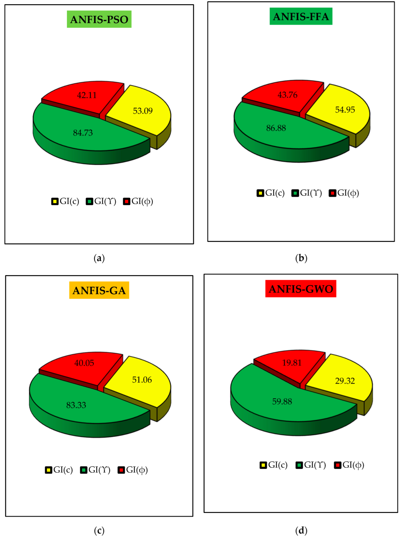
6.7. Gini Index (GI)

In this section, the relative significance of input parameters for prediction factor of safety against overturning is analyzed using the Gini index (GI). The Gini index of each input variable is computed, and the relative importance has been judged. A higher value of the Gini index means more significance of that individual input variable for the prediction of FOS. The Gini index for input parameters c (GI_c), φ (GI_φ) and Υ (GI_ϒ) can be computed as:

$$\mathrm{Gini} \mathrm{Index} ({\mathrm{GI}}_{\mathrm{c}})=|{\sum }_{\mathrm{i}=2}^{\mathrm{n}}{\mathrm{Cumc}}_{\mathrm{i}-1}{\mathrm{CumF}}_{\mathrm{i}}-{\sum }_{\mathrm{i}=2}^{\mathrm{n}}{\mathrm{Cumc}}_{\mathrm{i}}{\mathrm{CumF}}_{\mathrm{i}-1} |$$

(31)

$$\mathrm{Gini} \mathrm{Index} ({\mathrm{GI}}_{\mathsf{\phi }})=|{\sum }_{\mathrm{i}=2}^{\mathrm{n}}{\mathrm{Cum}\mathsf{\phi }}_{\mathrm{i}-1}{\mathrm{CumF}}_{\mathrm{i}}-{\sum }_{\mathrm{i}=2}^{\mathrm{n}}{\mathrm{Cum}\mathsf{\phi }}_{\mathrm{i}}{\mathrm{CumF}}_{\mathrm{i}-1} |$$

(32)

$$\mathrm{Gini} \mathrm{Index} ({\mathrm{GI}}_{\mathsf{\Upsilon }})=|{\sum }_{\mathrm{i}=2}^{\mathrm{n}}{\mathrm{Cum}\mathsf{{\rm Y}}}_{\mathrm{i}-1}{\mathrm{CumF}}_{\mathrm{i}}-{\sum }_{\mathrm{i}=2}^{\mathrm{n}}{\mathrm{Cum}\mathsf{{\rm Y}}}_{\mathrm{i}}{\mathrm{CumF}}_{\mathrm{i}-1} |$$

(33)

Here, Cumc, Cumφ, Cumϒ and CumF are the cumulative values of cohesion, angle of shearing resistance, unit weight of soil and predicted FOS against overturning, respectively.

In Figure 12, the relative significance of each input variable is shown by means of their Gini index. For all four proposed hybrid models, the Gini index values for all three input parameters, namely c, ϒ and φ, are shown in Figure 12. The Gini index value for unit weight of the backfill (ϒ) is higher among all three input parameters, followed by cohesion (c) and angle of shearing resistance (φ) for all four models. On the basis of their GI value, it can be clearly seen that ϒ is the most significant parameter, followed by c and φ for all four developed models.

7. Conclusions

In this research, reliability analysis of the gravity retaining wall is performed by taking c, Υ and φ as input variables, and the performance assessment parameters were computed for four hybrid ANFIS models. All four models were compared with numerous parameters such as statistical indices, R-curve, Williams plot, rank analysis and error matrix, and it showed that for the training phase, ANFIS-PSO gives a better result among all four models (ANFIS-PSO, ANFIS-FFA, ANFIS-GA and ANFIS-GWO), and for the testing phase, ANFIS-FFA gives better prediction power to compute FOS against overturning among all four models. In the training stage, the ANFIS-PSO model attained a total rank of 13 and outperformed the three models by far, while the ANFIS-FFA attained a total rank of 17 in the testing phase. However, when the comparison is made in terms of overall rank (Rank in training + Rank in testing stage) obtained by each model, ANFIS-PSO shows the highest predictive accuracy with an overall rank of 37, which is followed by ANFIS-FFA, ANFIS-GA and ANFIS-GWO. Reliability index (β) and probability of failure (P_f) is also computed for all four models and compared with the actual value. The ANFIS-PSO model gives a higher value of β and lower value of P_f among all the models. Apart from this, the Williams plot is drawn in order to know the applicability domain of the model. The Gini index value is also computed to analyze the influence of input parameters on FOS against overturning. The most influential parameters among the three input variables are unit weight of soil (ϒ), followed by cohesion (c) then angle of shearing resistance (φ).

References

1. Low, B.K.; Tang, W.H. Efficient Reliability Evaluation Using Spreadsheet. J. Eng. Mech. 1997, 123, 749–752. [Google Scholar] [CrossRef]
2. Chan, C.L.; Low, B.K. Practical second-order reliability analysis applied to foundation engineering. Int. J. Numer. Anal. Methods Géoméch. 2011, 36, 1387–1409. [Google Scholar] [CrossRef]
3. Cushing, A.G.; Whitman, J.L.; Szwed, A.; Nowak, A.S. Reliability analysis of anchored and cantilevered flexible retaining structures. In Limit State Design in Geotechnical Engineering Practice: (With CD-ROM); World Scientific: Singapore, 2003; pp. 1–38. [Google Scholar] [CrossRef]
4. Low, B.; Zhang, J.; Tang, W.H. Efficient system reliability analysis illustrated for a retaining wall and a soil slope. Comput. Geotech. 2011, 38, 196–204. [Google Scholar] [CrossRef]
5. GuhaRay, A.; Mondal, S.; Mohiuddin, H.H. Reliability Analysis of Retaining Walls Subjected to Blast Loading by Finite Element Approach. J. Inst. Eng. India Ser. A 2018, 99, 95–102. [Google Scholar] [CrossRef]
6. Alghaffar, M.; Wellington, C. Reliability analysis of retaining walls designed to British and European standards. Struct. Infrastruct. Eng. 2005, 1, 271–284. [Google Scholar] [CrossRef]
7. Kumar, A.; Roy, P. Reliability analysis of retaining wall using imprecise probability. In Proceedings of the 12th International Conference on Structural Safety and Reliability, Vienna, Austria, 6–10 August 2017; pp. 288–296. [Google Scholar]
8. Chouksey, S.K.; Fale, A. Reliability analysis of counterfort retaining wall. Int. J. Civ. Eng. Technol. 2017, 8, 1058–1073. [Google Scholar]
9. Cherubini, C. Probabilistic approach to the design of anchored sheet pile walls. Comput. Geotech. 2000, 26, 309–330. [Google Scholar] [CrossRef]
10. Yang, Z.; Ching, J. A novel simplified geotechnical reliability analysis method. Appl. Math. Model. 2019, 74, 337–349. [Google Scholar] [CrossRef]
11. Menon, D.; Mangalathu, S. Reliability analysis and design of cantilever RC retaining walls against sliding failure. Int. J. Geotech. Eng. 2011, 5, 131–141. [Google Scholar]
12. Wang, H.; Chen, H.; Wang, Y.; Han, L.; Li, H. Reliability analysis for stability of the gravity retaining wall under mountain torrent. Syst. Sci. Control Eng. 2020, 8, 434–440. [Google Scholar] [CrossRef]
13. Xiao, Z.-Q.; Huang, J.; Wang, Y.-J.; Xu, C.-Y.; Xia, H. Random Reliability Analysis of Gravity Retaining Wall Structural System. In Advances in Engineering Research, Proceedings of the 2014 International Conference on Mechanics and Civil Engineering (ICMCE-14), Wuhan, Chian, 13–14 December 2014; Atlantis Press: Amsterdam, The Netherlands, 2014; pp. 199–204. [Google Scholar] [CrossRef] [Green Version]
14. Zhang, D.B.; Sun, Z.B.; Zhu, C.Q. Reliability analysis of retaining walls with multiple failure modes. J. Cent. South Univ. 2013, 20, 2879–2886. [Google Scholar] [CrossRef]
15. Babu, G.L.S.; Basha, M. Optimum design of cantilever sheet pile walls in sandy soils using inverse reliability approach. Comput. Geotech. 2008, 35, 134–143. [Google Scholar] [CrossRef]
16. Low, B.K. Reliability-based design applied to retaining walls. Geotechnique 2005, 55, 63–75. [Google Scholar] [CrossRef]
17. Sun, J.; Yuefei, H. Modeling the simultaneous effects of particle size and porosity in simulating geo-materials. Materials 2022, 15, 1576. [Google Scholar] [CrossRef] [PubMed]
18. Sun, J. Hard particle force in a soft fracture. Sci. Rep. 2019, 9, 3065. [Google Scholar] [CrossRef]
19. Zhang, J.; Wang, Y. An ensemble method to improve prediction of earthquake-induced soil liquefaction: A multi-dataset study. Neural Comput. Appl. 2020, 33, 1533–1546. [Google Scholar] [CrossRef]
20. Harandizadeh, H.; Toufigh, M.M.; Toufigh, V. Application of improved ANFIS approaches to estimate bearing capacity of piles. Soft Comput. 2018, 23, 9537–9549. [Google Scholar] [CrossRef]
21. Zhang, W.; Goh, A. Multivariate adaptive regression splines for analysis of geotechnical engineering systems. Comput. Geotech. 2012, 48, 82–95. [Google Scholar] [CrossRef]
22. Mishra, P.; Samui, P.; Mahmoudi, E. Probabilistic Design of Retaining Wall Using Machine Learning Methods. Appl. Sci. 2021, 11, 5411. [Google Scholar] [CrossRef]
23. Zhang, W.; Zhang, Y.; Goh, A.T. Multivariate adaptive regression splines for inverse analysis of soil and wall properties in braced excavation. Tunn. Undergr. Space Technol. 2017, 64, 24–33. [Google Scholar] [CrossRef]
24. Xiang, Y.; Goh, A.T.C.; Zhang, W.; Runhong, Z. A multivariate adaptive regression splines model for estimation of maximum wall deflections induced by braced excavation in clays. Geomech. Eng. 2018, 14, 315–324. [Google Scholar]
25. Zhang, W.; Zhang, R.; Goh, A.T.C. Multivariate Adaptive Regression Splines Approach to Estimate Lateral Wall Deflection Profiles Caused by Braced Excavations in Clays. Geotech. Geol. Eng. 2017, 36, 1349–1363. [Google Scholar] [CrossRef]
26. Mishra, P.; Samui, P. Reliability Analysis of Retaining Wall Using Artificial Neural Network (ANN) and Adaptive Neuro-Fuzzy Inference System (ANFIS). In Proceedings of the Indian Geotechnical Conference 2019; Springer: Singapore, 2021; pp. 543–557. [Google Scholar] [CrossRef]
27. Ghani, S.; Kumari, S.; Bardhan, A. A novel liquefaction study for fine-grained soil using PCA-based hybrid soft computing models. Indian Acad. Sci. 2021, 46, 113. [Google Scholar] [CrossRef]
28. Zhang, W.; Goh, A.T. Multivariate adaptive regression splines and neural network models for prediction of pile drivability. Geosci. Front. 2016, 7, 45–52. [Google Scholar] [CrossRef]
29. Wang, L.; Wu, C.; Gu, X.; Liu, H.; Mei, G.; Zhang, W. Probabilistic stability analysis of earth dam slope under transient seepage using multivariate adaptive regression splines. Bull. Eng. Geol. Environ. 2020, 79, 2763–2775. [Google Scholar] [CrossRef]
30. Zhang, W.; Li, H.; Wu, C.; Li, Y.; Liu, Z.; Liu, H. Soft computing approach for prediction of surface settlement induced by earth pressure balance shield tunneling. Undergr. Space 2020, 6, 353–363. [Google Scholar] [CrossRef]
31. Wang, L.; Wu, C.; Tang, L.; Zhang, W.; Lacasse, S.; Liu, H.; Gao, L. Efficient reliability analysis of earth dam slope stability using extreme gradient boosting method. Acta Geotech. 2020, 15, 3135–3150. [Google Scholar] [CrossRef]
32. Wu, C.; Hong, L.; Wang, L.; Zhang, R.; Pijush, S.; Zhang, W. Prediction of wall deflection induced by braced excavation in spatially variable soils via convolutional neural network. Gondwana Res. 2022, in press. [Google Scholar] [CrossRef]
33. Yong, W.; Zhang, W.; Nguyen, H.; Bui, X.-N.; Choi, Y.; Nguyen-Thoi, T.; Zhou, J.; Tran, T.T. Analysis and prediction of diaphragm wall deflection induced by deep braced excavations using finite element method and artificial neural network optimized by metaheuristic algorithms. Reliab. Eng. Syst. Saf. 2022, 221, 108335. [Google Scholar] [CrossRef]
34. Takagi, T.; Sugeno, M. Derivation of fuzzy control rules from human operator’s control actions. IFAC Proc. Vol. 1983, 16, 55–60. [Google Scholar] [CrossRef]
35. Kennedy, J.; Eberhart, R. Particle swarm optimization. In Proceedings of the ICNN’95—International Conference on Neural Networks, Perth, WA, Australia, 27 November–1 December 1995; Volume 4, pp. 1942–1948. [Google Scholar]
36. Holland, J.H. Genetic algorithms. Sci. Am. 1992, 267, 66–72. [Google Scholar] [CrossRef]
37. Yang, X.S.; He, X. Firefly algorithm: Recent advances and applications. Int. J. Swarm Intell. 2013, 1, 36–50. [Google Scholar] [CrossRef]
38. Mirjalili, S.; Mirjalili, S.M.; Lewis, A. Grey wolf optimizer. Adv. Eng. Softw. 2014, 69, 46–61. [Google Scholar] [CrossRef]
39. Zhou, G.M.; Li, Y.; Zhang, F. Analysis of Reliability Calculation and System Analysis of Gravity Retaining Walls. Appl. Mech. Mater. 2014, 556–562, 862–866. [Google Scholar] [CrossRef]
Figure 1. Standard illustration of ANFIS structure.
Infrastructures 07 00121 g001
Figure 2. Gravity retaining wall considered for this study.
Infrastructures 07 00121 g002
Figure 3. Correlation plot among input variables (c, ϒ, φ) and response variable (FOS).
Infrastructures 07 00121 g003
Figure 4. Scatter plot among input parameters (a) c and FOS; (b) ϒ and FOS and (c) φ and FOS (variables are in normalized form).
Infrastructures 07 00121 g004
Figure 5. Methodology flowchart.
Infrastructures 07 00121 g005
Figure 6. Plot of actual and predicted FOS of training data (TR) for (a) ANFIS−GA; (b) ANFIS−PSO; (c) ANFIS−FFA; and (d) ANFIS−GWO models.
Infrastructures 07 00121 g006
Figure 7. Plot of actual and predicted FOS of testing data (TS) for (a) ANFIS−GA; (b) ANFIS−PSO; (c) ANFIS−FFA; and (d) ANFIS−GWO models.
Infrastructures 07 00121 g007
Figure 8. Williams plot for hybrid ANFIS model: (a) ANFIS−PSO, (b) ANFIS−FFA, (c) ANFIS−GA and (d) ANFIS−GWO.
Infrastructures 07 00121 g008
Figure 9. Accuracy matrix for hybrid ANFIS model (training and testing dataset).
Infrastructures 07 00121 g009
Figure 10. Error matrix for error measuring parameters (training and testing dataset).
Infrastructures 07 00121 g010
Figure 11. Error matrix for trend measuring parameters (training and testing dataset).
Infrastructures 07 00121 g011
Figure 12. The relative significance of input variables for (a) ANFIS-PSO, (b) ANFIS-FFA, (c) ANFIS-GA and (d) ANFIS-GWO model.
Infrastructures 07 00121 g012