1. Introduction
Bridges are key components of transport and infrastructural systems. Their safety is of paramount importance, considering that their disruption can have a high socio-economic impact and their failure can seriously endanger people’s lives [
1]. Vulnerability and risk analysis procedures for bridges are gaining more and more attention and the scientific literature on the topic is growing, with studies concerning various sources of hazards such as seismic [
2,
3,
4,
5] or flood-induced actions (e.g., scour) [
6,
7,
8].
To date, fragility curves represent a tool widely accepted by the community for the seismic performance assessment of any structural system (buildings and bridges). However, bridges are characterised by a wide spectrum of structural typologies (different static schemes) and potential failure modes (e.g., either ductile or brittle damage can develop on piers, abutments, bearing devices, and so on), and the failure scenario may vary substantially from case to case, especially for existing bridges designed according to inadequate seismic codes and methods.
Therefore, the information provided by fragility curves should not be too synthetic, otherwise, risk and loss may not be estimated properly. For instance, some common practices from past studies, such as estimating fragility curves based on a unique response parameter [
9,
10,
11] or cataloguing bridges within homogeneous fragility classes [
12,
13,
14], may be revealed as inadequate in view of the variability of the specificities of every single bridge structure, although these approaches are certainly useful for a preliminary or global scale analysis.
A detailed analysis of the bridge with its specific features is indeed required in the majority of cases, as also suggested by other authors [
15,
16]. The analysis of bridge fragility can be carried out by focusing either on the global performance of the bridge or on the single structural component response, and an “in-series” system assumption is often adopted for the global failure assessment of bridges [
15,
16,
17,
18,
19].
Some past studies addressed the problem of multiple critical components in seismic assessment by analysing the correlation between pairs of structural component responses and by proposing methodologies to develop probabilistic demand models [
20,
21,
22,
23,
24]. In particular, [
20,
21] focused their attention on the piers’ response by considering both flexural and shear mechanisms and their correlation effects on the bridge’s global fragility, but no other bridge elements were considered as contributing to the system failure. A step forward was made in [
22], where classical fragility curves were provided for a set of bridge components (one curve for each component) to assess the effectiveness of retrofit interventions. In [
23] a similar analysis typology was performed but it was extended at the network level. However, for the purpose of a detailed analysis of the bridge performance and the associated consequences, the evaluation of the contribution to the global fragility of all the failure mechanisms and their mutual relations, as well as the quantification of the damage extension over the bridge by focusing on a single component level, reveal very important information and none of the previous works have addressed these aspects. Finally, it is worth mentioning a relevant interesting study on this topic, i.e., [
24], in which the authors proposed conditional probability importance measures (CIMs) to account for the contribution of different bridge components to the system failure.
In the present paper, a novel easy-to-use and practical-oriented procedure for fragility analysis is proposed with the aim of providing a higher level of information about the possible failure mechanisms of existing bridges, overcoming some limits of classical approaches, and providing rapid and useful data to directly support the decision-making process (e.g., driving risk planning and management activities). More specifically, the proposed strategy is based on a novel organisation of the results coming from Multiple-Stripe Analysis (MSA) [
25], and it is conceived to perform two types of analysis having different but complementary objectives:
The failure mode analysis, consisting of a qualitative estimation of the most significant failure modes and related mutual relations, provides useful insights for the selection of the most suitable retrofit intervention.
The damage extent analysis, consisting of a quantitative assessment of the damage spreading over the system, is useful to perform loss analysis, prioritisation of repair interventions (e.g., within a given infrastructural network), and develop a rational design of retrofit strategies.
The presented method exploits basic probability theory concepts and manipulates them in order to provide, for each of the two tasks listed above, new typologies of fragility functions, namely, multiple damage fragility functions and damage extent fragility functions.
An illustrative application of the method is presented in a realistic case study, a multi-span simply supported reinforced concrete Link Slab (LS) bridge designed according to the Italian codes of the 1970s. This typology is widespread within the Italian infrastructural network [
26,
27] and can be commonly found in the infrastructural stock of many other countries such as Turkey or China [
28,
29,
30]. In this framework, the application also provides insights into the LS bridge’s seismic fragility. A bidirectional seismic input is used, and a stochastic ground motion model is exploited for the generation of sets of earthquake time series to perform nonlinear time history (TH) analyses within the MSA framework. The proposed strategy was revealed to be able to provide a clear overview of the most significant bridge failure modes and the damage extension on the bridge.
2. Proposed Methodology for the Fragility Analysis of Bridges
The methodology proposed below aims to achieve a deeper understanding of the most significant failure modes of the bridge by also highlighting their reciprocal relation and explicitly assessing the damage extent relevant to each mode.
Principal notations adopted throughout the paper are recalled below for the purpose of the presentation. Failure is herein defined as the attainment of unsatisfactory performance, and it is identified by the exceedance of a threshold value of a selected response parameter controlling the behaviour and the damage evolution of a key structural component. Different response parameters can be considered to control all the possible failure mechanisms of the bridge, which can affect piers, abutments, bearings, and so on.
A limit state is described by a set of thresholds relevant to different potential failure modes. Different limit states (sets of thresholds) can be of interest, according to different performance states of the structure, e.g., serviceability or ultimate conditions. Therefore, failures could occur in different components and concern different response parameters and thresholds exceedance (limit states). Limit states are considered one by one in the following.
For this study, failure events are grouped in families related to parameters of interest, and each family is denoted by a capital letter (e.g.,
A,
B,
C,…). For instance, we can suppose a bridge has the following failure modes:
A, pier flexural failure;
B, pier shear brittle failure; and
C, bearings failure due to maximum stroke attainment. A given failure mode (e.g.,
A) may occur in one or more components of the family and the failure of each component is denoted by
Ak, with
k = 1,…
NAk, where
NAk is the number of components that may suffer the type of failure
A. Consequently, the failure event
A occurs if at least one component experiences failure, i.e., one or more
Ak events occur:
Fragility functions can be used to specify the probability of failure (i.e., of any limit state of interest) of a system as a function of some seismic intensity measure,
IM (further discussed later). The fragility function relevant to event
, hereafter called the
Mode A-fragility curve, is defined as
while the fragility curve of a single element,
of the family
is denoted as the
Mode A component-fragility curve and is defined as follows:
Different failure modes (
A,B,C,…) are considered so that a
Global fragility curve,
FGfc, can be defined (Equation (4)) on the union event
U (with
U =
A∪
B∪
C…) denoting the global failure event).
Global fragility curves represent the typical output of the vulnerability analysis carried out according to the existing common practical approaches. Two novel types of analysis and organisation of the outcomes of a seismic analysis are proposed in this paper and discussed in the following sections: the failure modes analysis and the damage extent analysis, each providing different information about the system vulnerability, and a different contribution to the risk assessment and the decision-making process.
2.1. Failure Mode Analysis
The analysis is oriented to provide qualitative information about the bridge vulnerability, giving evidence of typical or recurrent failure modes. For this purpose, the (global failure) event
U is partitioned into subsets of disjoint events
Ml, with
l = 1,…
NM, considering all the
NM possible combinations of failure types, such as the occurrence of only one failure mode and the coupling of two or more failure modes. As an example, if three failure modes
,
and
are possible,
is partitioned into seven sets (
Figure 1):
U\(
B∪
C),
U\(
A∪
C),
U\(
A∪
B), (
A∩
C)\
B, (
B∩
C)
\A, (
A∩
B)\
C, and (
A∩
B∩
C).
The probability of occurrence of
is the sum of the probabilities of
Ml, i.e.,
and the function
characterises the fragility associated with the
l-th failure scenario (combination of given damage modes) and will thus be named the
Multiple damage fragility curve.
These types of fragility functions (i.e., based on the grouping of two or more failure modes) permit not only the highlighting of the most recurrent failure modes of the bridge but also the ability to investigate their probable interactions (probabilities of joint events and relevant variability with the seismic intensity). This information may be crucial to choose the most effective type of seismic risk mitigation strategy for the bridge.
2.2. Analysis of the Damage Extent
With reference to a specific failure mode, the analysis aims to provide a quantitative evaluation of the failure extent; the outcomes can be of interest for the assessment of seismic losses since reconstruction or repair costs depend on the effective number of components undergoing damage. In this case, the single failure type, e.g., A, is studied and the event is partitioned based on its NAk components to obtain information about the damage extent. This partition is based on the number of damaged elements, e.g., subsets Sm, m = 1…NS, that may concern failures occurring in 1 element, 2 elements, … all the NAk = NS elements. It is evident that each subset can collect failures of the same family occurring at different locations along the bridge because only the failure number is counted. In this sense, the approach is not able to provide information about the location of damage but only about the damage spreading.
The number of components is often high, and a rougher partition obtained by joining some subsets (i.e.,
NS <
NAk) is often convenient, considering situations in which failures involve increasing percentages of the elements of the family (e.g., up to 25%, from 25% to 50%, from 50% to 75% and from 75% to 100%). A schematic representation is given in
Figure 2, where the failure mode
A is studied and
S1,
S2,and
S3 are used for events involving damage in 25%, 50%, and 75% of the elements of the family.
Therefore, subsets of disjoint events
Dm can be considered such that,
with
ND being the total number of possible combinations. It follows that the probability of
A can also be defined as follows.
There are different postprocessing analyses that can be consequently performed, each aimed to highlight a specific perspective of the damage situation. One might be interested in the fragility curves of disjoint failure subsets
Relevant to specific intervals of damage extent (e.g., between 25% and 50% of damaged elements). One might be also interested in assessing how the probability of a specific damage condition (e.g., 25% damaged elements) varies over the seismic intensity levels, thus a fragility curve expressed by
can be used. Finally, the exceedance probability of a given damage condition can be expressed through the following fragility function
in which
denotes the complementary event of
.
2.3. Probabilistic Tools for the Proposed Methodology
The methodology proposed in the previous section requires a probabilistic tool to be combined with to collect the data for estimating fragility functions.
Different methods can be used [
25], such as Incremental Dynamic Analysis (IDA), Cloud analysis, and Multiple-Stripe Analysis (MSA) [
31]. In this work, the efficient and widely used MSA is suggested. It consists of performing several nonlinear dynamic analyses at different seismic intensity levels; unlike IDA, different acceleration time series are used at each
IM level, with the possibility of considering changes of the ground motion features with the seismic intensity [
32]. Recorded seismic events are frequently used for this purpose, requiring scaling or spectral matching procedures to achieve the target conditioning to the different intensity levels, operations which often lead to accelerograms with unrealistic features [
33]. More efficiently, a proper stochastic model can be adopted, overcoming the issue of scaling and lack of real high-magnitude records, especially at the highest
IM levels. The latter strategy is adopted in the present work, although the proposed methodology can be applied using recorded accelerograms as well.
In detail, the simple but exhaustive point-source spectrum model of Boore [
34] is herein exploited, in combination with the stochastic ground motion model of Atkinson-Silva [
35], for the generation of bidirectional seismic samples and the characterisation of the
IM hazard curve
νIM (
im), the latter denoting the Mean Annual Frequency (MAF) of exceeding a given value,
im, of the random variable,
IM. As for the choice of the
IM, the most practical and used ones for the 2D analysis of bridges are the Peak Ground Acceleration (PGA) [
15,
22] and the spectral acceleration S
a(1.0) at the period of 1.0 s [
36,
37]. The spectral acceleration Sa (T
1) can be used as well, where T
1 is the period of the first mode of vibration; however, this approach may suffer from the generally large difference between the longitudinal and the transverse periods of the bridge. To cope with this issue, an average period, T, between the transversal (1.15 s) and longitudinal vibration (0.67 s) modes is considered in this study. In order to account for the bidirectional nature of the seismic input (X and Y directions), the maximum spectral acceleration component at the period T is selected as the conditioning parameter [
38,
39], i.e.,
IM = max{S
a,X (T), S
a,Y (T)}.
It is worth noting that the record-to-record variability represents the most important source of uncertainty for the seismic response characterisation of bridges; the other sources of uncertainty (e.g., concerning the structural model, etc.) are thus neglected in this work, given the usually low influence on the response [
40,
41].
Fragility functions
F(im) are analytically evaluated from the output of MSA by following an EDP-based method in which either empirical or parametric approaches can be adopted. The former can be mathematically expressed as follows [
31,
42]:
where
is the total number of ground motion samples per
IM level and
Ik(im) is the indicator function (
Ik = 1 if a failure occurs at the
k-th time-history analysis for
IM =
im,
Ik = 0 otherwise). Alternatively, starting from the count of the fraction of records,
Nfi in each stripe causing failure, a parametric lognormal cumulative distribution,
can be fitted, which is a reasonable assumption for a large set of cases, whose parameters,
(
expressing the median of the fragility function and
β the standard deviation of the natural logarithm of
IM), can be evaluated by maximising the logarithm of the likelihood function [
43]:
with
NIM as the number of
IM levels. Both the empirical and the parametric approaches are used in this work.
2.4. Procedure Implementation
The algorithm for generating fragility curves according to the proposed strategy (which finds a formal mathematical definition in
Section 2.1 and
Section 2.2) is now explained by the means of two simple explicative examples having the role of aiding the interested reader in practical procedures implementation.
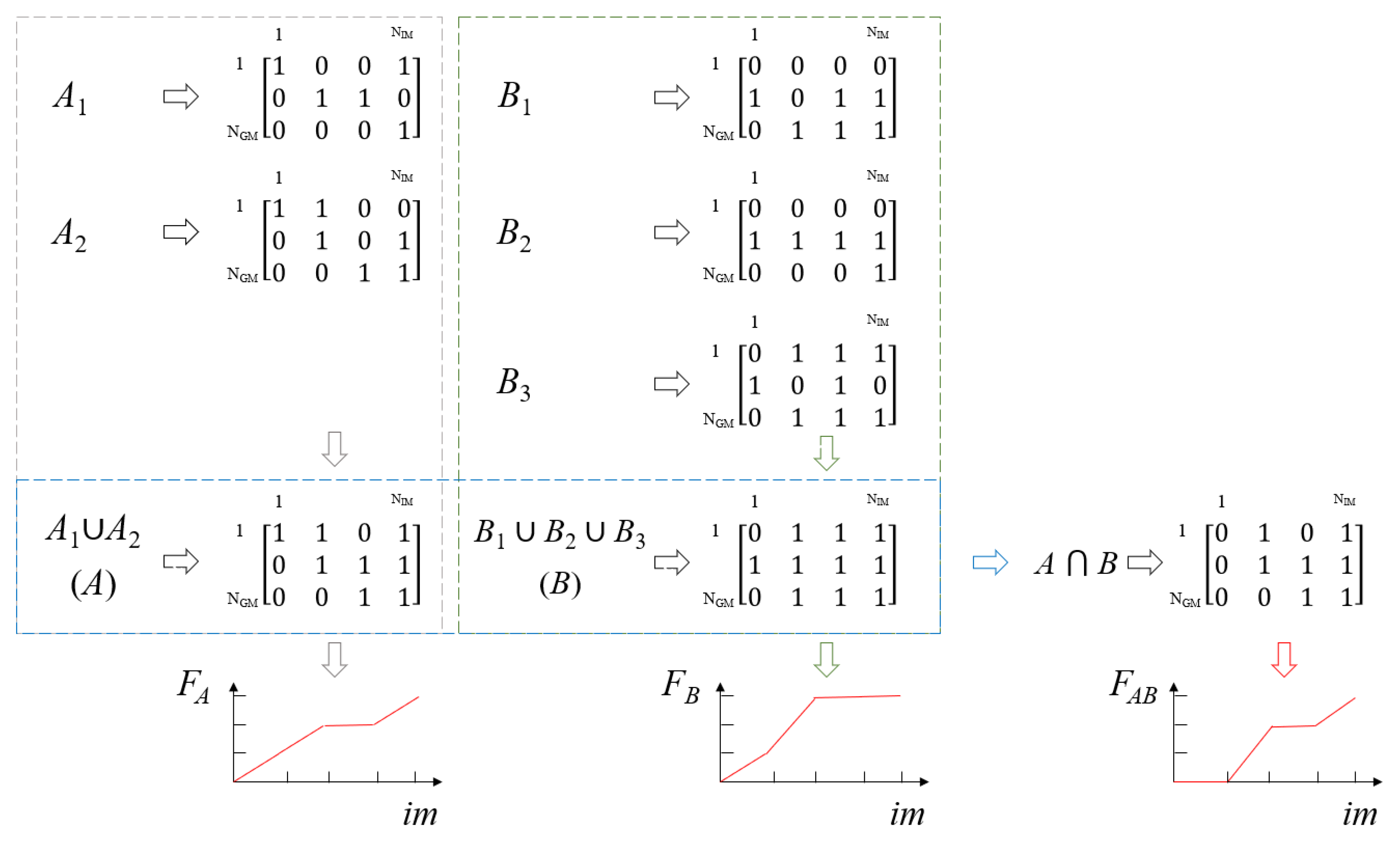
The procedure for building
multiple damage fragility functions is first presented, according to the schematic flowchart given in
Figure 3. For example, suppose having two element families,
A and
B, the former made of two sub-components (e.g., two piers) and the latter constituting three sub-elements (e.g., three kinematic link bars). We perform MSA analysis at four
IM levels by using three ground motion samples (the proposed case is deliberately chosen to be extremely simple at the expense of scarce physical significance) and we want to provide both single component fragility curves (
FA and
FB) and
multiple damage fragility curve FAB. The procedure can be summarised through the following steps:
- (1)
Consider family A; for each element (in this case, A1 and A2) a Boolean NGM × NIM matrix is built collecting 1 s for failure cases (i.e., the EDPs exceed a given threshold value) and 0 s otherwise.
- (2)
Compute the union A1∪A2, which is still a Boolean matrix and characterises the failure states of the whole family A (i.e., failure occurs if at least one component of the family fails).
- (3)
Steps 1 and 2 must be repeated for set B, here supposed to have three sub-elements, hence, three Boolean matrixes are first generated and then the union B1∪B2∪B3 is computed.
- (4)
The resulting union matrixes of A and B can be used individually to evaluate classical single component fragility functions (through either Equation (12) or (13)), i.e., FA and FB.
- (5)
Additionally, the intersection between the resulting union matrixes of A and B can be computed and used to estimate the multiple damage fragility function FAB, which adds information about the occurrence of simultaneous failures to the previous fragility types on the considered components.
The flowchart given in
Figure 4 can be followed concerning the procedure for extracting the
damage extent fragility functions. For example, suppose having the family
B from the previous example:
- (1)
For each element (B1, B2, and B3), a Boolean NGM × NIM matrix is built collecting 1 s and 0 s based on the same criterion presented in step 1 of the previous procedure.
- (2)
Compute the matrix sum B1 + B2 +B3, which is no longer Boolean and contains quantitative information on the number of components that failed in family B.
- (3)
Supposing we are interested in characterising the probabilities of having more than two elements at every IM level, a Boolean NGM × NIM matrix can be built collecting 1 s in the matrix positions where the values are higher than 2 and 0 s where the values are equal or lower than 2.
- (4)
The resulting matrix can be used to build a quantitative damage extent fragility function FB.
3. Case Study
3.1. Seismic Hazard
The seismic scenario is described by the point-source spectrum model of Boore [
34], combined with the stochastic ground motion model of Atkinson-Silva [
35]. The values of the parameters governing the stochastic ground motion model are set in order to provide an
IM hazard curve representative of medium-high seismicity in Italy (
Figure 5a).
Following the recommendations provided in [
31], the
IM curve of
Figure 5a is divided into 20 stripes equally spaced in the log-log plane (highlighted by red circle markers), with the relevant spectral acceleration values summarised in
Table 1. Moreover, a set of 20 ground motion pairs is selected for every
IM level to properly account for the record-to-record variability. For the sake of completeness, the response spectra of both the horizontal components of the seismic input conditional to two intensity levels (i.e.,
IM level 5 and
IM level 10, corresponding to return periods of 50 years and 450 years, respectively) are depicted in
Figure 5b,c.
3.2. Geometrical and Structural Details
A multi-span simply supported pre-stressed concrete bridge is considered in this paper to show the potential of the proposed methodology for fragility analysis. Geometrical and mechanical parameters of the case study are chosen to make it as accurate as possible and representative of a specific bridge class, in order to increase the general validity of the results for the bridge typology. In detail, reference is made to existing Italian bridges constructed in the 1970s, before the emanation of codes introducing seismic detailing and capacity design concepts.
The bridge deck is 130 m long, with five simply supported spans of 25 m each. The cross-section is composed of a cast-in-site slab (12.50 m wide) and three V-shape pre-stressed concrete girders (
Figure 6a). Neoprene bearing supports are installed (
Figure 6b), having the same semi-rigid mechanical behaviour along the two horizontal directions. Spans are connected at the slab level through kinematic links, made by a set of DYWIDAG bars of diameter Ø40 mm; the link zone between two adjacent spans is 200 mm long. A schematic representation of the links and a detail of the joint from a real design project [
44] are provided in
Figure 7. The bar arrangement at each link is determined consistently with the static scheme, having a fixed constraint located at the right abutment (
Figure 6c) for entrusting the longitudinal seismic actions. Moderately slender (10 m tall) RC piers with a circular cross-section of a diameter of 2 m are adopted (having a height/diameter ratio equal to 5). A schematic longitudinal view of the bridge is provided in
Figure 6d.
Gravity loads are derived directly from the deck self-weight, while permanent loads of the superstructure are estimated to be 50 kN/m. A simulated design has been performed according to the Italian Codes [
45,
46], considering both gravity and seismic loads. The latter is modelled as equivalent seismic forces applied separately along the transverse and longitudinal directions of the bridge. Piers are designed as cantilever elements subjected to forces derived from the masses of a single span while links are designed considering the cumulative contributions of the span masses, depending on the link position with respect to the fixed abutment. The equivalent seismic force
Fh, provided by the above codes, is 7% of the gravity loads. By assuming a concrete grade R
ck 300 (cubic characteristic strength equal to 30 MPa) and a steel grade FeB44k (yielding strength equal to 435 MPa), the simulated design requires 59 longitudinal steel rebars of diameter 26 mm for piers and Ø14 mm hoops equally spaced at 25 cm along the whole pier shaft. A longitudinal reinforcement ratio of 1% is assumed for the piers, compatible with the minimum amount required by the code (i.e., 0.6%, [
46]). Links are designed assuming the allowable design stresses foreseen by [
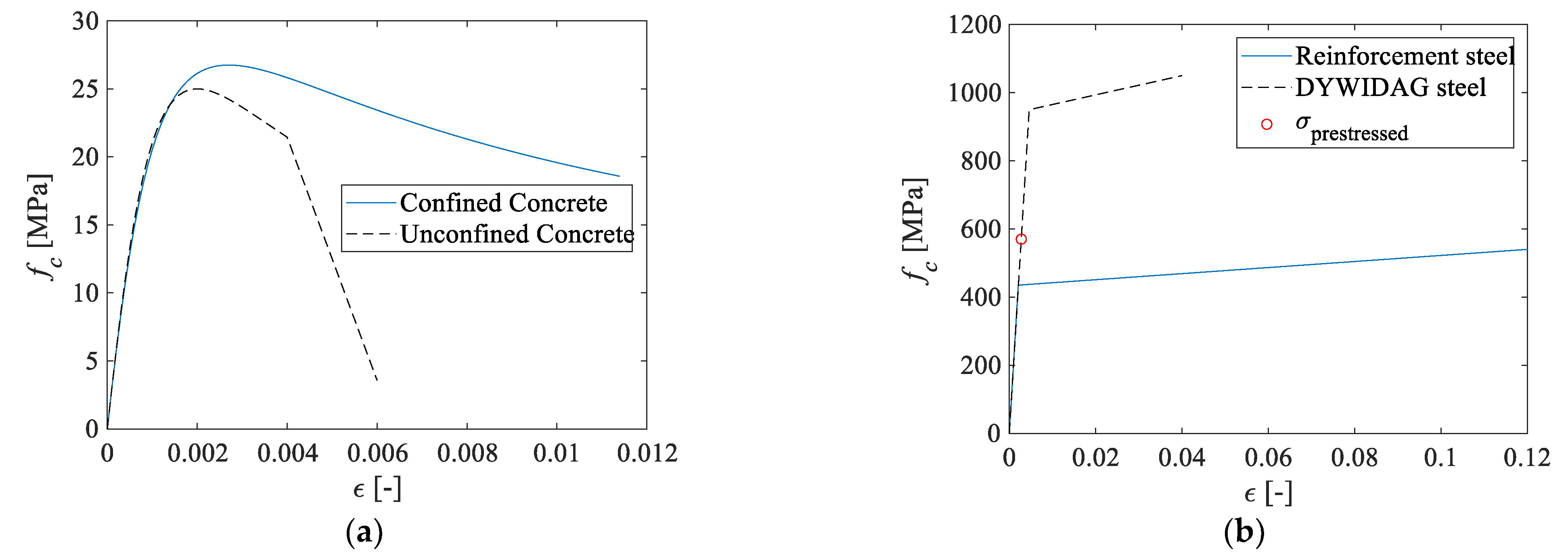
46] for prestressing steel. As for piers, the confinement effect due to stirrups is considered, assuming confined and unconfined compressive strength and ultimate strains for the cover and core concrete, respectively. The DYWIDAG bars are pre-tensioned at 60% of the steel yielding stress. For sake of completeness, the material constitutive laws are depicted in charts in
Figure 8, whereas material properties are reported in
Table 2.
Finally, to sustain gravity and permanent loads, neoprene bearings with supporting area
= 157.5 cm
2, thickness
= 52 mm, and shear modulus
= 1 MPa are adopted [
47].
3.3. Bridge Structural Model
A three-dimensional (3D) nonlinear model is developed in OpenSees [
48]. Deck girders are modelled as elastic beam elements [
17] with nonlinearity concentrated at the joints, within the kinematic links. Each kinematic link has a total length of 200 mm and is composed of DYWIDAG bars which are in part covered by the concrete (link portion inside the slab, 50 mm long) and in part uncovered (bare central part of the bars, 100 mm long) [
29]. According to this configuration, three in-series fibre section sub-elements are adopted to model the links: a straight layer of fibres with
Steel02 elastic-plastic behaviour and pretension stress (60% of yielding stress) are used for the DYWIDAG bars; and
Concrete01 material is used for the slab.
Bearings are modelled according to [
49] by means of
zero-length elements with
Steel01 uniaxial material and elastic stiffness
expressed as a function of the shear modulus
, the supporting area of the device
, and the device thickness
. The maximum force of the bearing is calculated as
, i.e., as the minimum between the force
related to the friction mechanism (
is the vertical load acting on the bearing and
is the sliding coefficient between the concrete surface and neoprene, assumed equal to 0.25), and the shear failure of the neoprene
(
is the maximum allowable shear strain for neoprene, assumed equal to 100%). In this case, the shear rupture of the neoprene pads governs the bearing failure.
Pier caps are assumed as rigid elements connecting the deck beam ends to the bearings. Columns are modelled using displacement-based fibre elements, able to account for the evolution of the plastic hinge at the base of the pier [
22]. Concrete is described by the
Concrete01 material, with parameters assumed according to Mander, Priestley, and Park [
50] (
Figure 8a); longitudinal steel rebars are introduced as line fibres with
Steel02 uniaxial material.
Seat-type abutments resting on piles are considered since this typology is the most widespread on the Italian road networks. The response of the abutments is modelled by evaluating the contribution of both the earth pressure and the structural stiffness in longitudinal and transverse directions. Along the longitudinal direction, the passive resistance mobilised at the abutment back wall is simulated using the hyperbolic soil model proposed by Shamsabadi et al. [
51], assuming a granular soil type. The active response in the longitudinal direction and the transverse forces are instead entirely assigned to piles, whose response is schematised with a trilinear force deformation law (
Figure 8b). Parameters characterising the pile constitutive law are determined following the design recommendations in [
52], assuming a 7 kN/mm/pile resistance and considering yielding force as the inertial force proportional to the mass of the entire bridge deck to be carried by the foundation piles.
The bilinear contact element developed by Muthukumar and DesRoches [
53] is used to model the pounding between the deck and the left abutment, as well as between adjacent spans after the rupture of the link bars at the ultimate strain. In fact, the link bar’s ultimate capacity is explicitly accounted for by the adoption of a
MinMax material that activates once the ultimate strain in the bars is attained.
Distributed masses on deck and pier elements are defined considering a density of 2.5 t/m3 for the RC and lumped nodal masses are instead used for the pier cap. Gravity and permanent loads are directly derived from distributed and nodal masses and applied before the Time History (TH) nonlinear analysis.
A graphical summary of the main details of the modelling strategy is given in
Figure 9. It is worth noting that the modelling strategy detailed in this Section was also validated by performing a comparison in terms of the modal properties (frequencies and mode shapes) between the two models of the bridge: the one developed in OpenSees and a less-refined model developed within commercial software (
Figure 10). The modal properties of the FE model in the commercial software derive from the Operational Modal Analysis results of an existing viaduct in Central Italy [
54].
3.4. Demand Parameters and Capacity Limits
The following demand parameters are monitored to assess the structural response of the bridge: (1) the pier top maximum displacement, controlling the pier ductile mechanism; (2) the bearings maximum displacement; (3) the maximum strain on the link-slab steel bars; (4) the abutment maximum longitudinal displacement for the soil passive response; (5) the abutment maximum longitudinal displacement for the soil active response; and (6) the abutment maximum transverse displacement. It must be noted that the plastic hinge status at the base of the pier is related to the pier top displacement through a suitable moment-curvature sectional analysis of the pier cross-section by assuming a cantilever system. Brittle failure on the piers is not considered because the shear capacity largely overcomes the shear demand (after the hinge opening) for the case study at hand.
Three Performance Levels (PLs) are assessed: the onset of an irreversible damage condition, denoted as d
y (e.g., piers or DYWIDAG bars yielding or sliding activation for bearings); the attainment of the ultimate capacity of the bridge component, denoted as d
u (e.g., the maximum stroke of the bearings, ultimate strains in the DYWIDAG bars or pier collapse); and an intermediate limit state, d
LS, is introduced to represent an extensive damage condition, related to the Life Safety limit state of the current code [
55].
The limit values for every performance level and bridge component (summarised in
Table 3) are based on literature studies [
36] (PLs for abutments), technical documents [
49] (bearings and piers) and seismic codes [
55]. Values assumed for the DYWIDAG bars are consistent with the specific steel grade.
4. Results and Discussion
This section presents the results stemming from the application of the proposed fragility analysis method to the selected case study. The bridge response is examined at different levels of detail. First, the fragilities of each family of elements and related failure modes are discussed (
Section 4.1) according to a classical fragility analysis procedure. Afterwards, fragility analysis is performed according to the proposed approach, with the aim of evaluating: (1) the mechanisms which most contribute to the bridge fragility (
Section 4.2), (2) their mutual interactions (
Section 4.2), and (3) the extent of damage over the bridge (
Section 4.3). Given the specific features of the considered case study, a unique failure mode can be identified for each system component (failures of bearings are only due to strokes, kinematic links failure is governed by the strain of the bar, and piers failure is governed by the pier head displacement). The only components showing three potential failure modes are the abutments, which are characterised by two longitudinal and one transverse failure mode; the three failure modes of the abutments will be enveloped in
Section 4.2 and
Section 4.3 to make the results discussion clearer.
4.1. Failure Modes and Global Fragility Analysis
According to the notation of
Section 2, the
Mode A-fragility function is defined according to Equation (2) and represents the envelope of the fragility curves of single elements
Ak contributing to the given failure mode
A. For the application of the proposed methodology to the present case study, the following quantities are defined:
Mode L-fragility curve characterising the failure of Link (L) bars;
Mode P-fragility curve for the Piers (P);
Mode B-fragility curve for the Bearings (B); and
Mode AP-,
Mode AA-, and
Mode AT-fragility curves characterising the failure of Abutments for Passive (AP), Active (AA), and Transverse (AT) mechanisms, respectively. In
Figure 11, the six failure mode fragility curves (L, P, B, AP, AA, and AT) are compared. Such a representation in the results is quite classical in fragility analysis and allows for the identification of some general trends of the bridge seismic response. For every performance level, the failure modes governing the fragility can be identified based on their relative position within the charts, i.e., ordered from the left (higher fragility) to the right (lower fragility). For the adopted case study, Links are the most vulnerable component while Piers are the less fragile ones. The level of detail of the results is sometimes further reduced by considering a
global fragility representation for every performance level, corresponding to the envelope of the single failure mode fragility curves of
Figure 11. According to this, the Link’s fragility curves would fully represent the fragility of the whole bridge under investigation. Previous considerations make it evident that in the limit of a classical analysis procedure a large amount of information remains hidden, such as: which link, or group of links, is more vulnerable among the family; how many components (e.g., number of Links) are experiencing failure; and which combination of failure modes (e.g., links and bearings) most govern the failure within a given interval of seismic intensities. To provide such a major level of detail to the bridge response characterisation, the fragility method proposed in
Section 2 should be applied, as presented hereafter.
4.2. Multiple Damage Fragility Analysis
As discussed in the previous sections, the knowledge of the relative probabilistic contribution provided by one or more failure mechanisms to the global fragility has great relevance, particularly for organising and managing repair interventions on the bridge. This information can be achieved through
multiple damage fragility curves (i.e.,
(Equation (6))), according to the analysis of the failure modes presented in
Section 2.1.
Since different numbers of mechanisms may undergo damage by varying the IM, multiple damage fragility curves do not necessarily have a monotonically increasing trend, and a broken-line representation is herein preferred.
Three sets of plots are reported in
Figure 12 to show the combination of damage mechanisms at the considered performance levels, and, for each of them, different charts are represented to provide a clearer view of the results. Capital letters, introduced in the previous section (i.e., P, L, B, and A), are used to denote the different mechanisms. In the charts, black thick solid lines represent the global fragility curves for damage, life safety, and collapse performance levels. The
multiple damage fragility curves are shown with thin solid lines with different colours for each combination of mechanisms. Only non-null fragility curves are shown in the figures.
Some illustrative comments are given below for the collapse limit state (
Figure 12c) to show the quality of information that can be derived from the proposed analysis. At the lowest seismic intensities (S
a (T)
0.5 g), link bars are the only components contributing to the collapse fragility (i.e., global fragility overlaps with links fragility); for higher intensities (0.5 g < S
a (T)
1.5 g), bearings start experiencing failure so that the bridge collapse is attained due to a combination of concurring failures on link bars and bearings together; at very high seismic intensities (S
a (T) > 1.5 g), slight participation of the abutments on the global collapse fragility can be observed. The knowledge of the most probable concurring failure mechanisms can help to select the best retrofit intervention and plan monitoring strategies. Moreover, knowing the range of
IMs at which specific failure combinations take place, more informed and focused post-earthquake in-situ inspections could be organised depending on the seismic intensity registered at the bridge location.
4.3. Analysis of the Damage Extent
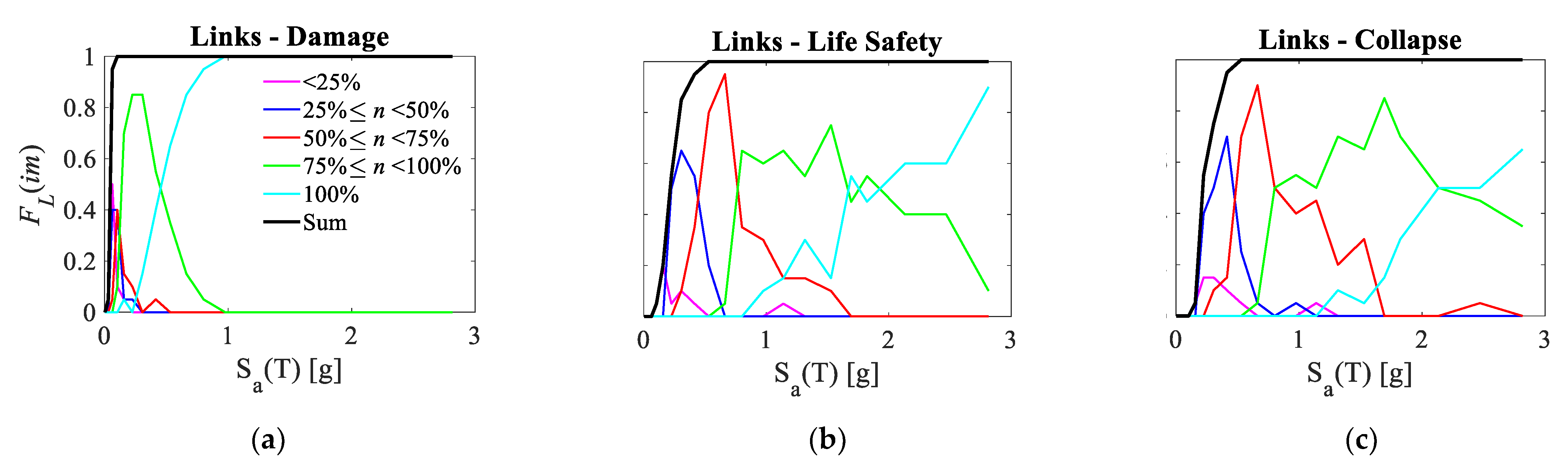
A quantitative evaluation of the damage extent, which may be of interest for the seismic loss assessment, is addressed in this Section. Three types of quantitative fragility functions are examined, as detailed in the next relevant Sections. Unfortunately, the presentation and the discussion of all three fragility types for all the bridge structural components are not feasible due to space limits. For this reason, only one component will be examined for each fragility typology: Type 1 fragility functions are provided for links; Type 2 fragility functions are presented for piers; and Type 3 fragility functions are provided for bearings.
4.3.1. Type 1 Quantitative Fragility Functions
This Section presents fragility curves for specific intervals of damage extent (e.g., between 25% and 50% of damaged elements) obtained by considering disjointed failure subsets according to Equation (9) of
Section 2.2. The current evaluation is performed on the number of individual link bars involved in the failure. Fragility curves for different percent intervals of damage extent are plotted in
Figure 13 and compared to the
Mode L-fragility curve (black thick solid line), representing the envelope (classical) fragility curve for the link bars, and also corresponding to the sum of all the single damage extent fragility curves (being the separated damage intervals and collectively exhaustive for the Links failure event
L).
Several pieces of information could be extracted by interpreting the results of
Figure 13.
For instance, it can be observed that in the range of low-medium seismic intensities (Sa (T) < 1.0 g), there is a quite high probability (up to 85%) that 75% to 100% of the link bars are slightly damaged (
Figure 13a); in the same
IM range, there is also a quite high probability (up to over the 90%) to observe severe damages (
Figure 13b) and collapses (
Figure 13c) on 50% to 75% of link bars. For the damage performance level, the condition of totally damaged link bars presents a high probability of exceedance (i.e., >50%) starting from Sa (T) = 0.5 g The failure condition involving 100% of the link bars has a significant probability of occurrence (i.e., >50%) starting from Sa (T) = 1.7 g (life safety performance level) and 2.1 g (collapse performance level).
4.3.2. Type 2 Quantitative Fragility Functions
Another possible way to organise the analysis results is by evaluating the probability of having exact percentages of failed bridge components, namely: 25%, 50%, 75%, and 100%. Results concerning the piers are shown in
Figure 14 for the damage performance level only. The envelope fragility curve (sum of the plotted quantitative curves) is also reported (black solid line). The highest contributions to the failure are relative to the cases of 50% and 100% piers damaged, with probabilities growing starting from 1.0 g of spectral acceleration. This means that the structural system is more prone to develop a rapid evolution of damage along the bridge rather than a gradual one. More specifically, for 1.0 g < S
a (T) < 2.0 g, the major contribution to the fragility of piers is that 50% of piers are damaged (blue line); at very high
IMs (i.e., S
a (T) > 2.0 g), the condition that all the piers exceed the damage condition is prevalent, with probabilities growing rapidly from about 40% to 80%.
4.3.3. Type 3 Quantitative Fragility Functions
This type of quantitative fragility curve is obtained by computing the probability of observing failure on a number of elements greater or equal to prefixed significative percent thresholds. For illustrative purposes, the family of bearing devices is analysed. Given the high number of elements, bearings are grouped in six sets, each corresponding to deck support (i.e., four sets relevant to piers and two sets relevant to abutments). To assess the damage extent, four percent thresholds are assumed (≥ 25%, ≥ 50%, ≥ 75%, and =100%), with the following correspondence in terms of bearing sets: ≥ two sets of bearings (≥ 25%); ≥ three sets of bearings (≥ 50%); ≥ four sets of bearings (≥ 75%); = six sets of bearings (= 100%).
The outcomes stemming from the analysis are shown in
Figure 15, according to which, the system shows a partially fragile behaviour at damage and life safety performance levels, with the probabilities of exceeding damage for 25% and 50% of the supporting device sets almost equal (compare magenta and blue curves). It is interesting to notice that whatever performance threshold is considered, the failure never involves 100 of the bearing sets.
5. Conclusions
Fragility analyses carried out according to common procedures are typically focused on the evaluation of the global performance of the bridge. They provide a synthetic characterisation of the failure probability of the system but hide the causes behind such failure propensity; the resulting knowledge of the actual bridge’s vulnerability might be thus insufficient for the quantification of the consequences and costs associated with seismic risk, and they are not very effective in supporting the decision-making processes related to seismic prevention.
In this paper, a systematic methodology for the evaluation of bridge fragility is proposed which exploits basic probability theory concepts and organises the results of a multi-stripe analysis. The proposed fragility analysis provides new typologies of “fragility functions”, which provide a higher level of information with respect to conventional fragility curves and make results available that can be more effectively used to plan prevention actions and to predict losses in post-event seismic scenarios.
More specifically, the following two typologies of fragility functions are presented, having different but complementary objectives: multiple damage fragility functions and damage extent fragility functions. The former provides information about the set of the most probable multiple mechanisms contributing to the failure of the bridge and it is of interest for planning effective strengthening actions. This way, the probabilistic information is not limited to the single damage mechanism, as it is common in fragility analysis, but it is extended to all the possible combinations of mechanism activation, hence useful information concerning their mutual correlation is provided as well. It is worth noting that the information extracted by applying this proposed fragility analysis can be conveniently used to choose the best repair action, optimise/prioritise the retrofit interventions in case of occurrence of an earthquake, or for maintenance purposes. In addition, by knowing the seismic intensity at which specific combinations of failure mechanisms are expected, more informed and focused post-earthquake in-situ inspections could be organised based on the real intensity of the occurred seismic event.
Concerning the latter fragility function proposed, three different strategies of results manipulation are presented, all aimed at a probabilistic characterisation of the damage extension of a given failure mechanism and useful to predict the extent of potential losses.
Moreover, the different types of fragility curves presented in this paper can be used within a broader probabilistic framework oriented to seismic risk estimation (i.e., exploiting the convolution integral between fragility and hazard) to perform life-cycle cost analysis and/or estimate the seismic losses. Moreover, the proposed methodology can be extended within frameworks oriented towards path-dependent seismic risk analysis, including ageing and degradation phenomena.
The mathematical formulation of tools proposed in this paper is first presented; then, details concerning the implementation of practical procedures are given, and finally, the methodology is applied to a realistic case study consisting of a reinforced concrete link-slab bridge.
Finally, despite the illustrative purpose of the presented application, some preliminary insights on the seismic fragility of this benchmark case study were obtained through the proposed analysis methodology, such as the extreme vulnerability of the link bars and the bearings. Future studies will be aimed to assess, through the proposed strategy, the vulnerability of other widespread bridge typologies (e.g., steel-concrete composite decks).
Author Contributions
Conceptualization, L.M., F.S., S.C., F.G. and A.D.; methodology, L.M., F.S., and A.D.; software, L.M. and F.S.; validation, L.M., F.S., S.C., F.G. and A.D.; formal analysis, L.M. and F.S.; writing—original draft preparation, L.M., F.S. and S.C.; writing—review and editing, L.M., F.S., S.C., F.G. and A.D.; visualization, L.M. and F.S.; supervision, F.S., S.C., F.G. and A.D. All authors have read and agreed to the published version of the manuscript.
Funding
This research received no external funding.
Conflicts of Interest
The authors declare no conflict of interest.
References
- Deodatis, G.; Ellingwood, B.R.; Frangopol, D.M. (Eds.) Safety, Reliability, Risk and Life-Cycle Performance of Structures and Infrastructures; CRC Press: Boca Raton, FL, USA, 2014. [Google Scholar]
- Tubaldi, E.; Scozzese, F.; De Domenico, D.; Dall’Asta, A. Effects of axial loads and higher order modes on the seismic response of tall bridge piers. Eng. Struct. 2021, 247, 113134. [Google Scholar] [CrossRef]
- Tubaldi, E.; Dall’Asta, A. A design method for seismically isolated bridges with abutment restraint. Eng. Struct. 2011, 33, 786–795. [Google Scholar] [CrossRef]
- Shekhar, S.; Ghosh, J. Improved component-level deterioration modeling and capacity estimation for seismic fragility assessment of highway bridges. ASCE-ASME J. Risk Uncertain. Eng. Syst. Part A Civ. Eng. 2021, 7, 04021053. [Google Scholar] [CrossRef]
- Kilanitis, I.; Sextos, A. Integrated seismic risk and resilience assessment of roadway networks in earthquake prone areas. Bull. Earthq. Eng. 2019, 17, 181–210. [Google Scholar] [CrossRef]
- Tubaldi, E.; Macorini, L.; Izzuddin, B.A.; Manes, C.; Laio, F. A framework for probabilistic assessment of clear-water scour around bridge piers. Struct. Saf. 2017, 69, 11–22. [Google Scholar] [CrossRef]
- Zampieri, P.; Zanini, M.A.; Faleschini, F.; Hofer, L.; Pellegrino, C. Failure analysis of masonry arch bridges subject to local pier scour. Eng. Fail. Anal. 2017, 79, 371–384. [Google Scholar] [CrossRef]
- Ragni, L.; Scozzese, F.; Gara, F.; Tubaldi, E. Dynamic identification and collapse assessment of Rubbianello Bridge. In Proceedings of the IABSE Symposium Guimarães 2019, Guimaraes, Portugal, 27–29 March 2019; pp. 619–626. [Google Scholar]
- Shinozuka, M.; Feng, M.Q.; Lee, J.; Naganuma, T. Statistical analysis of fragility curves. J. Eng. Mech. 2000, 126, 1224–1231. [Google Scholar] [CrossRef]
- Hwang, H.; Liu, J.B.; Chiu, Y.H. Seismic Fragility Analysis of Highway Bridges. Technical Report, Mid-America Earthquake Center CD Release 01–06. 2001. Available online: https://www.ideals.illinois.edu/items/9330 (accessed on 1 September 2022).
- Mackie, K.R.; Stojadinović, B. R-factor parameterized bridge damage fragility curves. J. Bridge Eng. 2007, 12, 500–510. [Google Scholar] [CrossRef]
- Nielson, B.G.; DesRoches, R. Seismic fragility curves for typical highway bridge classes in the Central and South-eastern United States. Earthq. Spectra 2007, 23, 615–633. [Google Scholar] [CrossRef]
- Ramanathan, K.; DesRoches, R.; Padgett, J.E. Analytical fragility curves for multispan continuous steel girder bridges in moderate seismic zones. Transp. Res. Rec. 2010, 2202, 173–182. [Google Scholar] [CrossRef]
- Mangalathu, S.; Jeon, J.S.; Padgett, J.E.; DesRoches, R. ANCOVA-based grouping of bridge classes for seismic fragility assessment. Eng. Struct. 2016, 123, 379–394. [Google Scholar] [CrossRef]
- Stefanidou, S.P.; Kappos, A.J. Methodology for the development of bridge-specific fragility curves. Earthq. Eng. Struct. Dyn. 2017, 46, 73–93. [Google Scholar] [CrossRef]
- Stefanidou, S.P.; Kappos, A.J. Bridge-specific fragility analysis: When is it really necessary? Bull. Earthq. Eng. 2019, 17, 2245–2280. [Google Scholar] [CrossRef]
- Nielson, B.G.; DesRoches, R. Seismic fragility methodology for highway bridges using a component level approach. Earthq. Eng. Struct. Dyn. 2007, 36, 823–839. [Google Scholar] [CrossRef]
- Nowak, A.S.; Cho, T. Prediction of the combination of failure modes for an arch bridge system. J. Constr. Steel Res. 2007, 63, 1561–1569. [Google Scholar] [CrossRef]
- Gehl, P.; D’Ayala, D. Development of Bayesian networks for the multi-hazard fragility assessment of bridge systems. Struct. Saf. 2016, 60, 37–46. [Google Scholar] [CrossRef]
- Lupoi, G.; Franchin, P.; Lupoi, A.; Pinto, P.E. Seismic fragility analysis of structural systems. J. Eng. Mech. 2006, 132, 385–395. [Google Scholar] [CrossRef]
- Gardoni, P.; Mosalam, K.M.; Der Kiureghian, A. Probabilistic seismic demand models and fragility estimates for RC bridges. J. Earthq. Eng. 2003, 7, 79–106. [Google Scholar] [CrossRef]
- Padgett, J.E.; DesRoches, R. Methodology for the development of analytical fragility curves for retrofitted bridges. Earthq. Eng. Struct. Dyn. 2008, 37, 1157–1174. [Google Scholar] [CrossRef]
- Ghosh, J.; Rokneddin, K.; Duenas-Osorio, L.; Padgett, J.E. Seismic reliability assessment of aging highway bridge networks with field instrumentation data and correlated failures, I: Methodology. Earthq. Spectra 2014, 30, 819–843. [Google Scholar] [CrossRef]
- Dueñas-Osorio, L.; Padgett, J.E. Seismic reliability assessment of bridges with user-defined system failure events. J. Eng. Mech. 2011, 137, 680–690. [Google Scholar] [CrossRef]
- Jalayer, F.; Cornell, C.A. Alternative non-linear demand estimation methods for probability-based seismic assessments. Earthq. Eng. Struct. Dyn. 2009, 38, 951–972. [Google Scholar] [CrossRef]
- Briseghella, B.; Siviero, E.; Zordan, T. A composite integral bridge in Trento, Italy: Design and analysis. In Proceedings of the IABSE Symposium: Metropolitan Habitats and Infrastructure, Shanghai, China, 22–24 September 2004; pp. 238–239. [Google Scholar]
- Minnucci, L.; Scozzese, F.; Dall’Asta, A.; Carbonari, S.; Gara, F. Influence of the deck length on the fragility assessment of Italian RC link slab bridges. In Proceedings of the 1st Conference of the European Association on Quality Control of Bridges and Structures, Padua, Italy, 29 August–1 September 2021. [Google Scholar]
- Caner, A.; Zia, P. Behavior and design of link slabs for jointless bridge decks. PCI J. 1998, 43, 68–81. [Google Scholar] [CrossRef]
- Sevgili, G.; Caner, A. Improved seismic response of multisimple-span skewed bridges retrofitted with link slabs. J. Bridge Eng. 2009, 14, 452–459. [Google Scholar] [CrossRef]
- Wang, C.; Shen, Y.; Zou, Y.; Zhuang, Y.; Li, T. Analysis of mechanical characteristics of steel-concrete composite flat link slab on simply-supported beam bridge. KSCE J. Civ. Eng. 2019, 23, 3571–3580. [Google Scholar] [CrossRef]
- Scozzese, F.; Tubaldi, E.; Dall’Asta, A. Assessment of the effectiveness of multiple-stripe analysis by using a stochastic earthquake input model. Bull. Earthq. Eng. 2020, 18, 3167–3203. [Google Scholar] [CrossRef]
- Bradley, B.A.; Cubrinovski, M.; Dhakal, R.P.; MacRae, G.A. Probabilistic seismic performance and loss assessment of a bridge–foundation–soil system. Soil Dyn. Earthq. Eng. 2010, 30, 395–411. [Google Scholar] [CrossRef]
- Goulet, C.A.; Watson-Lamprey, J.; Baker, J.; Haselton, C.; Luco, N. Assessment of ground motion selection and modification (GMSM) methods for non-linear dynamic analyses of structures. In Proceedings of the Geotechnical Earthquake Engineering and Soil Dynamics IV, Sacramento, CA, USA, 18–22 May 2022; pp. 1–10. [Google Scholar]
- Boore, D.M. Simulation of ground motion using the stochastic method. Pure Appl. Geophys. 2003, 160, 635–676. [Google Scholar] [CrossRef]
- Atkinson, G.M.; Silva, W. Stochastic modeling of California ground motions. Bull. Seismol. Soc. Am. 2000, 90, 255–274. [Google Scholar] [CrossRef]
- Ramanathan, K.N. Next Generation Seismic Fragility Curves for California Bridges Incorporating the Evolution in Seismic Design Philosophy. Doctoral Dissertation, Georgia Institute of Technology, Atlanta, GA, USA, 2012. [Google Scholar]
- Xie, Y.; DesRoches, R. Sensitivity of seismic demands and fragility estimates of a typical California highway bridge to uncertainties in its soil-structure interaction modeling. Eng. Struct. 2019, 189, 605–617. [Google Scholar] [CrossRef]
- Iervolino, I.; Spillatura, A.; Bazzurro, P. Seismic reliability of code-conforming Italian buildings. J. Earthq. Eng. 2018, 22, 5–27. [Google Scholar] [CrossRef]
- Pavia, A.; Scozzese, F.; Petrucci, E.; Zona, A. Seismic upgrading of a historical masonry bell tower through an internal dissipative steel structure. Buildings 2021, 11, 24. [Google Scholar] [CrossRef]
- Dolsek, M. Incremental dynamic analysis with consideration of modeling uncertainties. Earthq. Eng. Struct. Dyn. 2009, 38, 805–825. [Google Scholar] [CrossRef]
- Tubaldi, E.; Barbato, M.; Dall’Asta, A. Influence of model parameter uncertainty on seismic transverse response and vulnerability of steel—Concrete composite bridges with dual load path. J. Struct. Eng. 2012, 138, 363–374. [Google Scholar] [CrossRef]
- Pinto, P.E.; Giannini, R.; Franchin, P. Seismic Reliability Analysis of Structures; IUSS Press: Pavia, Italy, 2004. [Google Scholar]
- Baker, J.W. Efficient analytical fragility function fitting using dynamic structural analysis. Earthq. Spectra 2015, 31, 579–599. [Google Scholar] [CrossRef]
- Gara, F.; Regni, M.; Roia, D.; Carbonari, S.; Dezi, F. Evidence of coupled soil-structure interaction and site response in continuous viaducts from ambient vibration tests. Soil Dyn. Earthq. Eng. 2019, 120, 408–422. [Google Scholar] [CrossRef]
- Ministero dei Lavori Pubblici, D.M. 03.03.1975, Approvazione delle Norme Tecniche per le Costruzioni in Zone Sismiche; Official Italian Journal—G.U. n.93, 08.04.1975. Available online: https://www.legislazionetecnica.it/1013502/normativa-edilizia-appalti-professioni-tecniche-sicurezza-ambiente/d-min-llpp-03-03-1975 (accessed on 1 September 2022). (In Italian).
- Ministero dei Lavori Pubblici, D.M. 30.05.1972, Norme Tecniche Alle quali Devono Uniformarsi le Costruzioni in Conglomerato Cementizio, Normale e Precompresso ed a Struttura Metallica. Official Italian Journal—G.U. n.190, 22.07.1972. Available online: www.staticaesismica.it/normative/DM_30_05_1972.pdf (accessed on 1 September 2022). (In Italian).
- CNR (Consiglio Nazionale delle Ricerche). Apparecchi di Appoggio per le Costruzioni. Istruzioni per L’impiego (CNR 10018); Technical Research Document; Consiglio Nazionale delle Ricerche: Rome, Italy, 1999. (In Italian) [Google Scholar]
- McKeena, F.; Fenves, G.; Scott, M. Open system for earthquake engineering simulation (OpenSees). In Pacific Earthquake Engineering Research Center; University of California: Berkeley, CA, USA, 2015. [Google Scholar]
- DSTE/PRS & UNIBAS—Autostrade per l’Italia S.p.A. Manuale Utente della Procedura AVS per la Valutazione della Vulnerabilità e Rischio Sismico dei Ponti e Viadotti Autostradali, Technical Research Document—In Verifiche sismiche NTC 2018—V01, version 2.1; Autostrade per l’Italia: Rome, Italy, 2019.
- Mander, J.B.; Priestley, M.J.; Park, R. Theoretical stress-strain model for confined concrete. J. Struct. Eng. 1998, 114, 1804–1826. [Google Scholar] [CrossRef]
- Shamsabadi, A.; Rollins, K.M.; Kapuskar, M. Nonlinear soil–abutment–bridge structure interaction for seismic performance-based design. J. Geotech. Geoenviron. Eng. 2007, 133, 707–720. [Google Scholar] [CrossRef]
- Caltrans SDC. Caltrans Seismic Design Criteria; California Department of Transportation: Sacramento, CA, USA, 2015. [Google Scholar]
- Muthukumar, S.; DesRoches, R. A Hertz contact model with non-linear damping for pounding simulation. Earthq. Eng. Struct. Dyn. 2006, 35, 811–828. [Google Scholar] [CrossRef]
- Roia, D.; Regni, M.; Gara, F.; Carbonari, S.; Dezi, F. Current state of the dynamic monitoring of the “Chiaravalle viaduct”. In Proceedings of the 2016 IEEE Workshop on Environmental, Energy, and Structural Monitoring Systems (EESMS), Bari, Italy, 13–14 June 2016; pp. 1–6. [Google Scholar]
- EN 1998-2; Eurocode 8: Design of structures for earthquake resistance—Part 2: Bridges. European Committee for Standardization: Brussels, Belgium, 2005.
Figure 1.
Analysis of failure modes corresponding to a global failure (event U): an example with three failure modes A, B, and C.
Figure 1.
Analysis of failure modes corresponding to a global failure (event U): an example with three failure modes A, B, and C.
Figure 2.
Analysis of the damage extent for failure mode A, different subsets of damaged components.
Figure 2.
Analysis of the damage extent for failure mode A, different subsets of damaged components.
Figure 3.
Flowchart for the multiple damage fragility functions estimation.
Figure 3.
Flowchart for the multiple damage fragility functions estimation.
Figure 4.
Flowchart for the damage extent fragility functions estimation.
Figure 4.
Flowchart for the damage extent fragility functions estimation.
Figure 5.
(a) IM hazard curve and relevant IM levels; response spectra of the horizontal components of seismic samples at two intensity levels; (b) Tr = 50 years; (c) Tr = 450 years.
Figure 5.
(a) IM hazard curve and relevant IM levels; response spectra of the horizontal components of seismic samples at two intensity levels; (b) Tr = 50 years; (c) Tr = 450 years.
Figure 6.
View of the example bridge. (a) Pre-stressed concrete deck cross-section; (b) scheme of link bar arrangement at the slab level (c) static scheme of bearings for abutments and piers; and (d) longitudinal view of the bridge.
Figure 6.
View of the example bridge. (a) Pre-stressed concrete deck cross-section; (b) scheme of link bar arrangement at the slab level (c) static scheme of bearings for abutments and piers; and (d) longitudinal view of the bridge.
Figure 7.
(
a) Schematic representation of debonded rebar link slab and (
b) detail of the joining elements between the decks (link slabs). Source:
design project of the road links among SS76 road, A14 highway, Falconara airport, and SS16 road, ANAS, 18.02. 1986 [
44].
Figure 7.
(
a) Schematic representation of debonded rebar link slab and (
b) detail of the joining elements between the decks (link slabs). Source:
design project of the road links among SS76 road, A14 highway, Falconara airport, and SS16 road, ANAS, 18.02. 1986 [
44].
Figure 8.
(a) Concrete constitutive laws; (b) Steel constitutive law.
Figure 8.
(a) Concrete constitutive laws; (b) Steel constitutive law.
Figure 9.
Details of the finite element model of the bridge: (a) deck, link slabs, bearings, and piers; (b) abutments and pounding.
Figure 9.
Details of the finite element model of the bridge: (a) deck, link slabs, bearings, and piers; (b) abutments and pounding.
Figure 10.
Three-dimensional view of the finite element model of the bridge.
Figure 10.
Three-dimensional view of the finite element model of the bridge.
Figure 11.
Failure mode fragility curves compared at specific performance levels: (a) damage; (b) life safety; and (c) collapse.
Figure 11.
Failure mode fragility curves compared at specific performance levels: (a) damage; (b) life safety; and (c) collapse.
Figure 12.
Multiple damage fragility curves at (a) damage; (b) life safety; and (c) collapse performance levels; envelope global fragility curves depicted by black solid lines.
Figure 12.
Multiple damage fragility curves at (a) damage; (b) life safety; and (c) collapse performance levels; envelope global fragility curves depicted by black solid lines.
Figure 13.
Type 1 quantitative fragility functions for link-slab bars: probabilities of occurrence of damage mechanisms for different percentages of involved links at (a) damage; (b) life safety; and (c) collapse performance levels.
Figure 13.
Type 1 quantitative fragility functions for link-slab bars: probabilities of occurrence of damage mechanisms for different percentages of involved links at (a) damage; (b) life safety; and (c) collapse performance levels.
Figure 14.
Type 2 quantitative fragility functions for piers: probabilities of occurrence of damage mechanisms for different percentages of involved piers at collapse performance levels.
Figure 14.
Type 2 quantitative fragility functions for piers: probabilities of occurrence of damage mechanisms for different percentages of involved piers at collapse performance levels.
Figure 15.
Type 3 quantitative fragility curves at (a) slight damage; (b) life safety; and (c) collapse performance levels for bearings: increasing percentages of involved elements (sets of devices).
Figure 15.
Type 3 quantitative fragility curves at (a) slight damage; (b) life safety; and (c) collapse performance levels for bearings: increasing percentages of involved elements (sets of devices).
Table 1.
Correspondence between IM levels and spectral accelerations (in g).
Table 1.
Correspondence between IM levels and spectral accelerations (in g).
| IM levels | 1 | 2 | 3 | 4 | 5 | 6 | 7 | 8 | 9 | 10 |
| Sa (T = 0.9) | 0.004 | 0.030 | 0.063 | 0.103 | 0.157 | 0.225 | 0.306 | 0.415 | 0.531 | 0.663 |
| IM levels | 11 | 12 | 13 | 14 | 15 | 16 | 17 | 18 | 19 | 20 |
| Sa (T = 0.9) | 0.802 | 0.976 | 1.140 | 1.316 | 1.529 | 1.693 | 1.823 | 2.134 | 2.470 | 2.816 |
Table 2.
Steel and concrete mechanical properties.
Table 2.
Steel and concrete mechanical properties.
| | DYWIDAG Steel Bars | Steel Reinforcement | Confined
Concrete | Unconfined
Concrete |
|---|
| Elastic modulus (MPa) | 206,000 | 206,000 | 30,000 | 30,000 |
| Yielding/Peak strength (MPa) | 950 (σprestress = 60% yielding) | 435 | 26.75 | 25.00 |
| Ultimate strength (MPa) | 1050 | 540 | 18.57 | 3.58 |
| Yielding/Peak strain (-) | 0.0046 | 0.00207 | 0.0027 | 0.002 |
| Ultimate strain (-) | 0.04 | 0.12000 | 0.0114 | 0.0060 |
Table 3.
Performance levels and related demand threshold values for the bridge components.
Table 3.
Performance levels and related demand threshold values for the bridge components.
| Performance Level (PL) | Link Bars
εbar (-) | Piers
up (m) | Bearings
ub (m) | Abutment-Passive
uAB-P (m) | Abutment-Active
uAB-A (m) | Abutment-Transverse
uAB-T (m) |
|---|
| Yielding/Damage (dy) | 0.0046 | 0.077 | 0.080 | 0.037 | 0.00975 | 0.00975 |
| Life Safety (dSL) | 3/4 εbar,u | 3/4 up,u | 3/4 ub,u | 1.000 | 0.0072 | 0.0072 |
| Collapse (du) | 0.0400 | 0.234 | 0.200 | 1.000 | 1.000 | 1.000 |
| Publisher’s Note: MDPI stays neutral with regard to jurisdictional claims in published maps and institutional affiliations. |
© 2022 by the authors. Licensee MDPI, Basel, Switzerland. This article is an open access article distributed under the terms and conditions of the Creative Commons Attribution (CC BY) license (https://creativecommons.org/licenses/by/4.0/).


 ,
, 


