Review

State-of-the-Art Review on Probabilistic Seismic Demand Models of Bridges: Machine-Learning Application

by
Farahnaz Soleimani
1 and
Donya Hajializadeh
2,*
1
Georgia Institute of Technology, School of Civil and Environmental Engineering, Atlanta, GA 30309, USA
2
Department of Civil and Environmental Engineering, University of Surrey, Guildford GU2 7XH, UK
*
Author to whom correspondence should be addressed.
Infrastructures 2022, 7(5), 64; https://doi.org/10.3390/infrastructures7050064
Submission received: 4 April 2022 / Revised: 21 April 2022 / Accepted: 22 April 2022 / Published: 24 April 2022
(This article belongs to the Special Issue Structural Performances of Bridges)

Abstract

:
Optimizing the serviceability of highway bridges is a fundamental prerequisite to provide proper infrastructure safety and emergency responses after natural hazards such as an earthquake. In this regard, fragility and resilience assessment have emerged as important means of describing the potential seismic risk and recovery process under uncertain inputs. Generating such assessments requires estimating the seismic demand of bridge components consisting of piers, deck, abutment, bearing, etc. The conventional probabilistic model to estimate the seismic demands was introduced more than two decades ago. Despite an extensive body of research ever attempting to improve demand models, the univariate demand model is the most common method used in practice. This work presents a comprehensive review of the evolution of demand models capturing machine-learning-based methodologies and their advantage in comparison to the conventional model. This study sheds light on understanding the existing demand models and their associated attributes along with their limitations. This study also provides an appraisal of the application of probabilistic demand models to generate fragility curves and subsequent application in the resilience assessment of bridges. Moreover, as a sound reference, this study highlights opportunities for future development leading to enhancement of the performance and applicability of the demand models.

1. Introduction

Demand models are principal components of the performance-based assessment of bridges in which their behavior is evaluated in a postulated seismic hazard scenario. In this process, various sources of aleatory and epistemic uncertainties [1] are involved that are considered in the probabilistic seismic demand analysis (PSDA) [2]. This leads to developing probabilistic seismic demand models (PSDMs), initially introduced by Shome et al. [3], from which fragility curves are generated to provide the probability of exceeding discrete levels of bridge performance. Both PSDMs and fragility curves are used in loss estimation, resilience analysis, and lifecycle assessment. Thereby, how well a PSDM predicts seismic demands directly governs the outcome of risk assessment and subsequent inferences and decisions. Nonetheless, developing or selecting a practical framework for PSDM is a challenging task itself.
To estimate the seismic demand of bridge components consisting of piers, deck, abutment, bearing, etc., the PSDMs were initially formulated about two decades ago. For a particular bridge component and a specific engineering demand parameter (EDP), this formulation provides an estimate of the median value of the demand as a power-law function of a ground motion intensity measure (IM), while it is formed based upon the log-normality assumption of the seismic demands [3,4]. For decades, this conventional form of PSDM has been widely used in the seismic risk analysis of bridges in practice. However, thriving advanced statistical and machine-learning methodologies have led to developing more efficient yet simple PSDMs with the most influential set of predictors. The conventional model can be improved in multiple aspects. For example, from a structural point of view, additional sources of uncertainties such as bridge modeling parameters can be incorporated into the formulation. Additionally, instead of using a single intensity measure, additional ground-motion (GM) characteristics can be counted in the list of predictors. From a statistical analysis point of view, the prediction accuracy of the models can be improved by applying more advanced and promising ML algorithms.
ML methodologies and their applications have evolved drastically over recent years to handle large-scale, complex problems. Consequently, natural hazards engineering is benefiting from the promise of ML approaches to facilitate decision making. In essence, PSDMs can be substantially improved by leveraging ML methods to manage complex datasets, treat various sources of uncertainties, and propose computationally efficient solutions. While a substantial body of research has been conducted during the recent decade to enrich the conventional model, none was found as the most superior one, and the implementation of ML in this domain is still in its early stages. Furthermore, each study is limited to a specific bridge type, a certain number of random variables as the predictors, selective model formats (linear or nonlinear), certain ML or statistical approaches, and specific assumptions. Moreover, there is a clear need to explore the improvements that have been conducted in this space and create an overview of the existing PSDMs that can be useful for research and practice. This can further support structural and bridge engineers to choose the most suitable PSDM based on the requirements in the existing models and the particularities in a real-world problem. Toward advancing PSDMs, it could be beneficial for researchers to determine the best way to expand the formulation by understanding which factors have been considered and which aspects need further investigation.
PSDMs are extensively used in the process of fragility analysis and resilience assessment of bridges. In this process, demand models are combined with the capacity and hazard models to describe structural performance. The general framework is presented in Figure 1 to provide an overview of the entire process, from generating probabilistic seismic demand models to their application in quantifying resilience. Collectively, the literature contains a wide range of definitions, metrics, and measurement techniques for infrastructure resilience quantification; however, there is a consensus in all proposed approaches in which resilience is defined as a function of the key performance indicator that best describes the performance of an asset. As demonstrated in Figure 1, in a PSDM-based resilience assessment, the resilience index is a function of both performance function/indicator/curve and the fragility analysis. Section 3 provides a critical review of the application of demand models in deriving the fragility curves and different techniques in resilience index quantification.
To address the aforementioned needs, this study presents a comprehensive state-of-the-art review of the proposed alternative demand models along with an explanation of their progress and theoretical aspects, advantages they offer over the conventional model, assumptions considered, and challenges. In particular, this study is interested in the efforts made toward applying machine-learning algorithms to improve bridge PSDMs and mainly focuses on the fundamental attributes of applying different methods rather than a critique of the mathematical frameworks. The existing models are compared in the context of their performance, simplicity, considered sources of uncertainty, GM characteristics counted in the model, and development complexity. Furthermore, the study presents an overview of the application of probabilistic seismic demand models and fragility curves in risk and resilience assessment. As the implementation of ML methods is growing, this study elucidates potential opportunities to promote a broader application of ML advances in enhancing PSDMs as a part of addressing needs in natural hazards engineering.

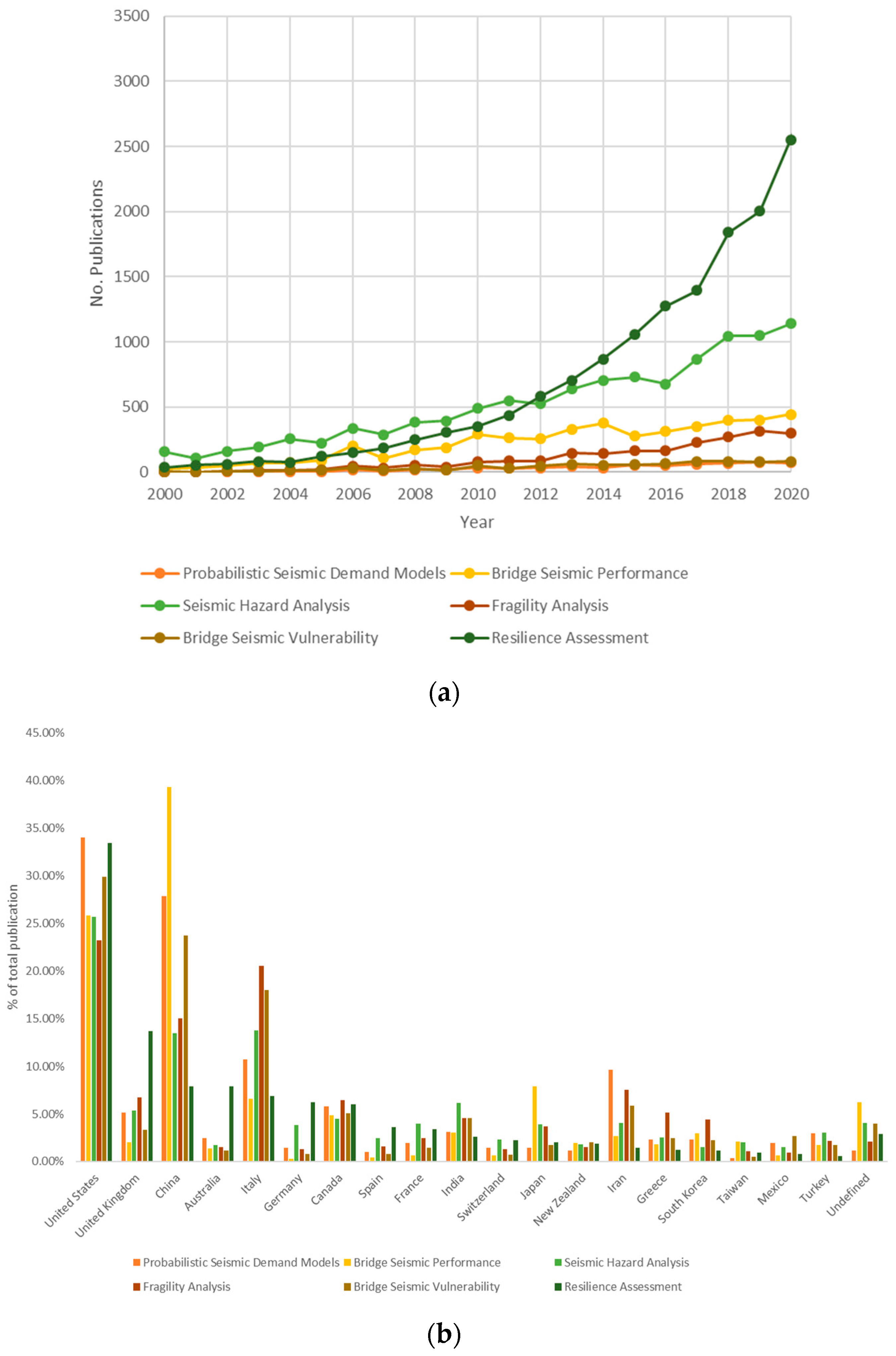
Literature Search Strategy

A structured search strategy was employed to provide an overview of the state-of-the-art literature on machine-learning applications in probabilistic seismic demand models. Our literature review focused on machine-learning approaches and probabilistic seismic demand models, specifically for bridges with the identified keywords: ‘probabilistic seismic demand models’, ‘bridge seismic performance’, ‘bridge seismic vulnerability’, ‘bridge seismic resilience’, ‘seismic hazard analysis’, ‘fragility analysis’, and ‘resilience’. Whilst there is a wide range of studies considering different hazards and different structure types, for the current study, the selected sources were preprocessed to focus the review on seismic hazards (earthquakes) and their impact on bridges.
For the purpose of this study, three literature lists were considered and critically reviewed. These include a primary list of literature following a direct search using the identified keywords. The second list includes the citation from the primary list to perform a forward search, and the reference in both former lists was used for the backward search. Figure 2 provides an overview of the temporal and spatial distribution of the search findings for each keyword.
Our literature sources include all published journal articles, conference proceedings, and well-cited technical reports. The temporal scope of the search was limited to all publications between 2000 and 2020. For this study, Google Scholar and Scopus were used as search engines. Following the initial screening (to assess the relevance to the subject domain), the combined final literature content resulted in a list of 97 articles, proceedings, and reports, and are provided in the reference list.

2. Seismic Vulnerability Assessment Using PSDMs

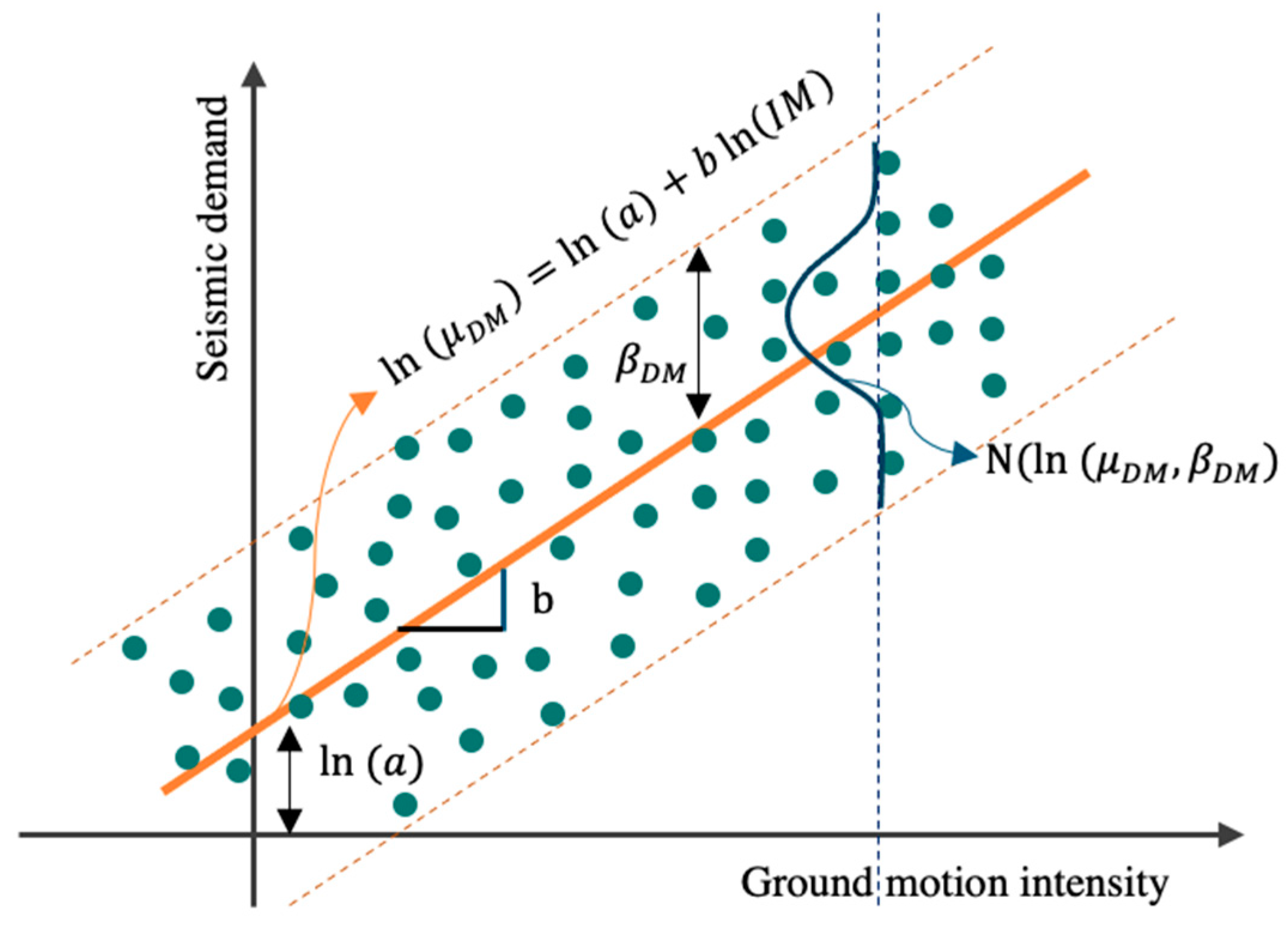
2.1. Description of PSDM and Univariate Linear Model

Defining performance objectives, commonly introduced as the mean annual frequency of decision variable (DV) exceeding a predefined limit value z (Equation (1) [4]), are essential elements to inaugurate a probabilistic performance-based framework. This annual probability is aggregated from measuring damage (DM > y) for EDP conditional to the seismic intensity measure (IM > w), assuming that these components are mutually independent. The parameters y and w correspond to the damage threshold/limit state corresponding to the bridge component and the ground motion intensity of interest corresponding to the bridge location, respectively.
v D V ( z ) = y   w   G D V | D M ( z | y ) | d G D M | I M ( y | w ) | d λ I M ( w )
To this end, Mackie and Stojadinovic [2] presented the development procedure of PSDM for typical highway overpass bridges. In their study, PSDM expressed demands as a function of IMs. They defined an optimal PSDM to be practical, sufficient, effective, and efficient. Effectiveness of a PSDM is defined as being able to find a closed-form solution [4] for Equation (1). To satisfy such a criterion, a log-normal distribution is assumed [3,5] for the structural demand based on which the conventional demand model was formed by a power-law model as Equation (2), where a and b are the regression coefficients, to estimate the median value of demand.
μ D M = a ( I M ) b
To build a practical PSDM, there should be a direct correlation between the demands simulated by the dynamic analysis and practical engineering quantities. To this end, known GM parameters need to be used, yet the relation between IM and EDPs should be independent of the GM characteristics to establish a sufficient PSDM.
Essential steps are required for the successful development of practical and sufficient PSDMs [2], including prudent choice of: a proper suite of GM, an appropriate measure of GM intensity, structural seismic demand measures, and a suitable range of bridge modeling parameters. The PSDMs are typically formulated by statistical analysis of the results of nonlinear dynamic analysis (time history analysis (THA) or incremental dynamic analysis (IDA)) of bridges exposed to a suite of GMs. The GMs need to be selected in an unbiased manner and in a way to capture the seismicity of the region where the bridge is located.
The initial and simplest PSDM formulation introduced in Equation (2) is equivalent to a univariate linear regression model in log–log coordinate space (Figure 3). This linear relationship is expressed in Equation (3), which has been extensively used for decades by researchers to analyze the seismic demand of bridges with various configurations (e.g., [6,7,8,9,10,11]). The variability in the demand values is expressed in terms of dispersion β D M (Equation (4)), which is calculated from the natural logarithm of the regression residuals. In the performance evaluation of the PSDMs, a small dispersion value indicates the model’s efficiency.
ln ( μ D M ) = ln ( a ) + b ln ( I M )
β D M = i = 1 n [ ln ( S D i ) ( ln ( a ) + b   l n ( I M i ) ) ] 2 n 2
In Equations (3) and (4), S D represents the value of seismic demand obtained from nonlinear dynamic analysis, and n is the total number of recorded responses. Although researchers used different IMs in their proposed PSDMs, a unified conclusion has not been made among them to recommend a single IM for bridges. For example, Freddi et al. [12] found spectral acceleration at 1.0 s period (Sa(1.0 s)) and peak ground velocity (PGV) as the most efficient structure-independent IMs, while Ma et al. [13] noted peak ground acceleration (PGA) as the best IM for the drift ratio model of the bridge columns. More discussion on this topic is provided later in the Discussion section.

2.2. Alternative Statistical Models for Seismic Demand Regression

Although the traditional PSDM is known as the simplest model for developing demand models of bridge components, it suffers from several limitations that can lead to inaccurate prediction of the demands and questionable reliability of the associated fragility and resilience evaluations. Researchers attempted to improve the traditional formulation of PSDMs (explained in the previous section) in several different aspects by using diverse approaches. In one aspect, over the years, researchers improved bridge models (e.g., [14,15]). Utilizing the latest bridge modeling and analysis tools provide the feasibility of incorporating prevailing sources of epistemic and aleatory uncertainties [16] inherent in the process of PSDA. In another aspect, sensitivity studies around the choice of GMs (near-field versus far-field) (e.g., [13]) and pertinent characteristics (e.g., [17]), soil conditions (e.g., [18]), geometric and material parameters (e.g., [19]), irregularities in a bridge configuration (e.g., [20]), pier shapes (e.g., [21]), and bridge portfolios (e.g., [22]) helped to understand how the bridge seismic performance is sensitive to these variations. In this section, we differentiate the progress paths of enhancing probabilistic demand models according to the implemented algorithms. The theoretical aspects of the models considered by different researchers are briefly described in each subsection, while details of the demands investigated, the uncertain parameters considered and the ground motion intensity measures, class of bridges studied, and the methodologies implemented are provided in Table 1. Table 2 provides the key aspects of reviewed literature.
A few studies (e.g., [11,23,24]) slightly modified the original formulation of PSDM by involving additional terms. As an example, Ma et al. [13] added a multiplicative factor, as a function of the fundamental period ( T ) of the bridge, to both constant and coefficient of the PSDM in log–log space. The proposed empirical model for the considered EDP, the maximum drift ratio at the top of piers of the studied single-column regular concrete bridge, was expressed as:
ln ( μ D M ) = ln ( a ) [ 10 4.36 T + 1.1 T 2 ] + b [ 10 1.82 T + 0.36 T 2 ] ln ( S a )
Another example is the corrective term introduced by Gardoni et al. [6], Choe et al. [40], Zhong et al. [41], and Huang et al. [23] using a Bayesian approach. For example, Huang et al. [23] presented this framework for the seismic deformation, shear, and bivariate deformation–shear demands of RC bridges with one single-column bent. The corrective terms are added to the commonly used deterministic demand models to produce probabilistic models and to moderate the bias. The corrective term as expressed in Equation (6) is a function of model parameters including unknown parameters. Huang et al. [23] adopted Bayesian updating to assess the unknown model parameters and select the correction terms, accordingly. To find an optimal corrective term, a set of explanatory functions were considered, from which γ was formed with respect to the structural properties and the GMs characteristics.
S D ( x ,   Θ ) = d ^ ( x ) + γ ( x , θ ) + σ ε
In Equation (6), d ^ represents the calculated demand by the deterministic model. In addition, x is a vector of input parameters (such as material properties, member dimensions, and boundary conditions); Θ is a vector of unknown modeling parameters (i.e., θ ) of the deterministic model and its standard deviation ( σ ); and ε stands for a normal random error with zero mean and unit variance.
Many researchers utilized the traditional form of PSDM to investigate the influence of irregular configurations such as skew angle (e.g., [11,42]), curvature (e.g., [43,44]), and tall or nonuniform column heights (e.g., [45,46,47]) on the produced PSDMs of bridges. As an example, Tondini and Stojadinovic [43] evaluated the bridge drift ratio of curved five-span box-girder concrete highway overpass bridges with single circular column bents using both nonlinear static and dynamic responses. The demand in the transverse direction was significantly affected by the bridge deck radius, while this effect was negligible in the longitudinal direction. In line with findings from Freddi et al. [12], Tondini and Stojadinovic [43] found structure-dependent IMs (e.g., Sa(T1)) more efficient than the independent IMs as the former ones induce smaller dispersion values. Among the studies that focused on irregular bridges, a few introduced modifications to the PSDMs.
A more complex modification of PSDMs for irregular bridge configurations was proposed by Soleimani [11] in which both constant and coefficient terms of the traditional PSDM (Equation (2)) were replaced by functions of the geometric irregularity parameters ( τ ) such as skew angle, column heights taller than the normal range, and unequal stiffness between the frames (Equation (7)). Linear functions were found as the best format to be used since monotonic trends were observed between the changes in demands and the variations of the irregularity parameters. The Levenberg–Marquardt method and Bayesian updating were implemented to optimize function parameters.
μ D M = ( a 0 + a 1 τ ) ( I M ) ( b 0 + b 1 τ )

2.3. Multivariate Linear Regression and Feature Selection Techniques

The widely used conventional form of PSDM (Equation (3)) expresses the relation between a single response variable (i.e., estimated seismic demand ( S ^ D )) and a single predictor variable (i.e., IM). This form can be extended to multivariate linear regression (MLR) that relates a single response to multiple predictors. The generated response surface models (RSM) can replace complex and time-consuming computational models (e.g., FEMs). Further, the MLR can be extended to a more general format using multivariate multiple linear regression (MMLR) (e.g., [48]) in which a vector of response variables within the same structure is expressed as a function of a vector of predictor variables. Basically, the latter two models yield equal regression coefficients and residual variance for individual responses. The advantage of using MMLR is automatically computing the residual correlation between the responses, which is beneficial for joint calculation of response measures in the process of damage estimation.
As an extension of univariate PSDMs, researchers proposed MLR-based PSDMs to incorporate the effect of structural modeling parameters together with the geometric and material properties of bridges. Although including all associated random variables and sources of uncertainties seem logical, including all variables in the model increases the risk of data overfitting, complexity, and computational time [49]. Hence, a few of the previous works (e.g., [17,18,20]) moved a step forward and implemented feature selection techniques to optimize the generated MLR.

2.3.1. Stepwise Regression

Researchers incorporated feature selecting techniques to identify the most influential subset of predictor variables to be included in the final PSDM. Stepwise regression [50] has been used for this purpose, in which the variables are either included or excluded in a sequence to optimize a fitness criterion. Once feature selection is utilized, an amendment is typically required in accordance with engineering judgment [17] to avoid overfitting and choosing many similar or correlated features and to revise the features on a physically reasonable basis.
Beginning with the simplest case that is in line with the traditional PSDM format, Xie et al. [17] adopted a generalized linear model (GLM) algorithm (Equation (8)) and stepwise technique for the regression modeling of seismic demands related to single-column highway bridges with rocking isolation. In this formula, α T is the vector of coefficients in the GLM, and x is the vector of input parameters. The variable ε is the normal random error. To estimate the uplift demand, stepwise regression identified PGV for the GM intensity measure and two additional GM parameters including velocity frequency measure and duration-based measure as influential parameters. Other significant factors in predicting demands were the rocking and the column vibrational parameters.
S ^ D = α T x + ε

2.3.2. LASSO

The least absolute shrinkage and selection operator (LASSO) [51] is a feature selection technique based on the linear regression algorithm. This approach minimizes the regression residuals by adding a constraint on the regressors’ coefficients, as shown in Equation (9). This constraint, which is known as the L1 norm regularization, allocates zero values to some of the coefficients, and as a result, the respective features are eliminated from the regression model. In Equation (9), n and k show the number of observations and the number of input parameters, and λ * corresponds to the hyperparameter.
min i = 1 n ( S D i j = 1 k α j x i j ) 2 + j = 1 k λ * || α j || 1
To this end, Soleimani et al. [20] applied LASSO to detect the modeling random variables with the most significant impact on the probabilistic seismic demands. The modeling variables corresponding to the bridge column specifications were identified as the most influential factors in predicting the seismic responses of bridges with geometric irregularities.
Similarly, Xie and DesRoches [18] performed a sensitivity analysis of the seismic demands of a typical two-span highway bridge in California with respect to the variations of 18 random variables corresponding to the soil-structure interaction (SSI) parameters. The SSI parameters were added to the regression demand model in addition to the IM. The two applied feature selection techniques for the linear models including stepwise and LASSO regression provided a comparable predictive capacity to the ordinary least squares regression model. The sensitivity study revealed that demands and fragility components related to the bridge foundations and abutment elements (e.g., unseating, bearing, and shear key) are significantly sensitive to the SSI parameters, whereas the results corresponding to the superstructure elements such as the column and deck are negligibly influenced by the variations in the SSI parameters.

2.4. Seismic Vulnerability Methodology Using Polynomial RSM

A group of researchers (e.g., [25,26]) considered second-order polynomials to generate PSDMs for developing regional seismic fragility curve of bridges. These models are formulated as in Equation (10) in which x i and x j represent input parameters (or predictor variables) and α 0 ,   α i , and α j are the constant term and the regression coefficients.
S ^ D = α 0 + i = 1 k α i x i + i = 1 k j = 1 ,   j i k α i j x i x j
Compared to the linear regression model, Pan et al. [27] attained a better fit by applying a second-order regression model on the response data of a multispan I-girder steel highway bridge, the most typical of continuous bridges in New York State. Different input variables were used in the regression models. As expressed in Equation (11), in the quadratic model, a bridge response was derived from PGA representing the IM. Using MLR, the response is expressed as a function of GM moment magnitude and distance (see Equation (12)). Specifically, the authors do not recommend using linear regression for earthquakes stronger than 0.6 g (PGA) since a nonlinear trend was observed beyond this range.
S ^ D = a ( ln ( P G A ) ) 2 + b ( ln ( P G A ) ) + c
S ^ D = a ( ln ( M w ) ) + b ( ln ( R ) ) + c
In line with the application of poly RSM, Seo and Linzell [25,28,29] focused on horizontally curved steel I-girder bridges. In addition to the PGA, they used macro- and micro level parameters as the input parameters of the model. More specifically, geometric and structural parameters (macro level) consisted of the number of spans, maximum span length, deck width, maximum column height, the radius of curvature, and girder spacing. The microlevel parameters included damping ratio, concrete compressive and tensile strength, Young’s modulus of concrete and reinforcements, and yield strength of reinforcements. Among these, the influential parameters in developing the bridge response models were detected to be the number of spans, maximum span length, the radius of curvature, and girder spacing [28,29]. Models were created to estimate bridge responses including column curvature ductility, abutment deformation, and radial and tangential bearing deformation. Moreover, it was observed that the number of spans, radius of curvature, and the maximum span length had the highest influence on the seismic fragilities [25].
On the basis of second-order polynomial equations, Park and Towashiraporn [30] developed RSM on steel-plate-girder bridges in Korea, considering the PGA and the variables describing the physical configuration of the bridge such as the number of spans, span length, and pier height. Initially, a simple sensitivity test was conducted on the influence of these variables on the bridge responses. This was done in an iterative process for each variable by changing the values of the variable of interest while fixing the value of the remaining variables at their median. Based on the results, bridge damage had a positive correlation (i.e., a linearly increasing trend) with pier height and PGA. Similarly, bridge damage exacerbated for a greater number of spans, particularly for two- to four-span bridges. The study showed that the sensitivity decreased for bridges with more than four spans. In contrast, the seismic damage was not sensitive to the span length variation. Thereby, PGA, pier height, and the number of spans were chosen as the input variables for the RSM, since they significantly affected the seismic damage of the studied bridge. Using the quadratic RSM, Seo and Park [31] generated fragility curves for a portfolio of regional curved-steel I-girder bridges in the Eastern United States. The constructed RSMs estimate the curvature ductility of the bridge columns, maximum deformation of bearing, and abutment as a function of PGA as the IM.
As stated, the polynomial RSMs have been mostly implemented on the seismic demand models of the steel girder bridges. As an example of a few works focused on the concrete bridges, Du et al. [32] utilized the second-order polynomial RSM (PRSM) approach to identify the optimal IM used in PSDMs. An optimization process was proposed to determine how adaptive intensity measures reduce the variability of demand models. In the case of the multispan simply supported concrete bridge, the one-parameter adaptive IMs, particularly the peak fractional ground response, improved the PSDMs. Despite that, similar results were observed whether the nonadaptive or one-parameter adaptive IMs were used in the models. However, a two fractional-order IM (i.e., the spectral acceleration (Sa(T*, ζ*)) at the optimal period T* and optimal damping ratio ζ* proposed by Shafieezadeh et al. [52] significantly improved the models. Polynomial orders higher than two have been rarely considered to estimate S D . Such examples are the works in the context of surrogate models that are explained in a later section.

2.5. Random Forest

Tree-based machine-learning algorithms have rarely been applied to derive PSDMs, which could be because the other algorithms are easier to interpret. Nevertheless, these algorithms have a couple of advantages over the other approaches. For instance, they can easily capture a nonlinear relation between the input and output variables without any prior assumption on the variable distributions. These algorithms construct decision trees by defining cut points for the values of the input variables and setting up targets for those cut points. Random forest (RF) is one of the well-known, widely used tree-based algorithms in which multiple random decision trees are generated, and the results are averaged [53].
Mangalathu and Jeon [33] used RF for a case study of three- and four-span concrete bridges with the characteristics corresponding to the California bridges. The seismic demands studied were related to the column curvature ductility and the displacements of abutments and bearings. Another advantage of RF is ranking how each of the input variables is important in predicting the model output. Using this feature, Mangalathu and Jeon [33] found the geometric modeling parameters such as the span length, deck width, and column height ranked as the most important parameters by RF. This finding is in agreement with the findings from other studies [20,47] on identifying the influential parameters in the process of developing PSDMs.

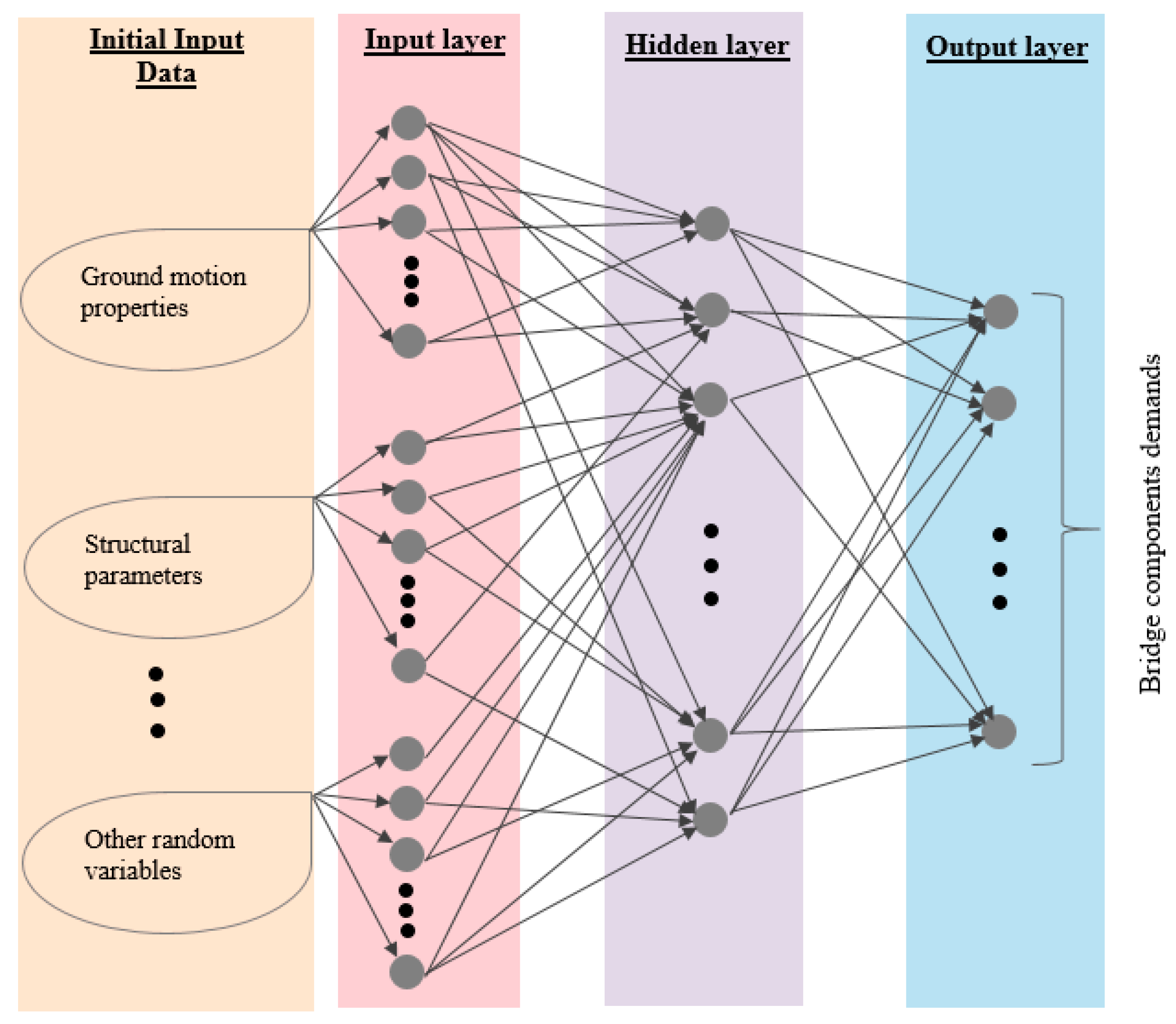
2.6. Artificial Neural Network

Artificial neural network (ANN) has been used in a few studies (e.g., [26,35,36,39]) to estimate S D . Although this algorithm has different model types, the multilayer perceptron (MLP) [54], the radial basis function (RBF) [55], and normalized RBF (NRBF) [56] have been explored.
This algorithm creates a fully interconnected network composed of three types of layers (Figure 4) each for the input variables, a hidden layer to map input and output, and the output layer. To estimate S D , the input layer consists of uncertain geometric, material, and GM parameters. The hidden layer includes a number of nodes (also known as neurons) that are trained to efficiently link the input layer to the output layer. The output layer has the bridge component response from which S ^ D is derived, based on Equation (13).
S ^ D = φ 0 + i = 1 m φ i ϕ i [ . , x ]
In this formulation, φ 0 is the bias and the φ i s are the connection weights between the layers. The values of these weights are iteratively set. The ϕ i [ . , x ] is a nonlinear mapping from the input layer to the hidden layer corresponding to the ith hidden layer of neurons. The main difference between the different network types lies in the type of mapping functions that are implemented by the neurons in the hidden layer. In the MLP network type, various mapping functions are used, such as the sigmoid transfer function (see Equation (14), where ω i j represents the weights assigned for the activity of the jth input parameter linked to the ith neuron).
ϕ i [ ω , x ] = 1 1 + exp ( j = 1 k ω i j x j )
The commonly adopted radial basis function is the Gaussian function as displayed in Equation (15) (for RBF) and Equation (16) (for NRBF), in which c r i stands for the centers of the radial basis functions and ζ i represents a scalar parameter corresponding to the width of the ith radial unit to the maximum distance found between the centers of the basis functions. In this function, the response monotonically changes as the distance from the central point increases. In Equation (16), the activity of neurons is normalized by the total activity of all m hidden neurons.
ϕ i [ c r , x ] = exp ( j = 1 k ( x j c r i j ) 2 2 ζ i 2 )
ϕ i [ c r , x ] = exp ( j = 1 k ( x j c r i j ) 2 2 ζ i 2 ) / i = 1 m ϕ i [ c r , x ]
Pang et al. [35] applied the aforementioned ANN algorithm with the RBF mapping functions and using 16 selected material and geometric parameters to estimate S D values of a three-span continuous bridge with two columns per bent, located in China. The considered demands were related to the displacements of the column, bearing, and abutment. They found that ANN could provide an acceptable approximation of the demand with less computational time compared to the traditional approach. Similarly, Mangalathu et al. [36] applied ANN with the MLP functions to two-, three-, and four-span concrete box-girder bridges with one and two columns per bent and seat type abutments. They used EDPs similar to those used by Pang et al. [35] and, by applying ANN, also found higher prediction accuracy than the conventional approach. Both of these studies used one hidden layer and a certain pre-assumed number of nodes in the layer (e.g., Mangalathu et al. [36] used 10 nodes). Some other researchers [26,39] implemented ANN in the context of the surrogate model that is explained in the following section.

2.7. Surrogate Models

Surrogate demand models (SDMs) for bridges, called also metamodels [57], were proposed by Ghosh et al. [26] with the intention to reduce computation time, yet efficiently reflect the complex relationship between predictor variables and the predicted seismic responses of a bridge component. To this end, Ghosh et al. [26] implemented four algorithms to approximate S D of multispan simply supported concrete bridges. These algorithms were the classical second-order PRSM (Equation (10)), multivariate adaptive regression splines (MARS) (introduced by Friedman [58]), and RBF networks (Equation (15)). They adopted a polyharmonic spline (Equation (17)) for the RBF. In the MARS algorithm (Equations (18) and (19)), S D is expressed as an expansion of spline basis functions, which are composed of linear and cubic splines. In these formulations, nbf represents the number of basis functions and nf represents the number of truncated linear functions multiplied in the ith basis function. The variable t j i is the knot value corresponding to the input parameter x j i and is set by a forward–backward iterative procedure. In addition, s j i is a sign variable that is equal to +1 or −1, which indicates the right or left side of the considered step function.
ϕ i [ ω , x ] = j = 1 k ( x j c r i j ) 2 ζ i 2
S ^ D = ρ 0 + i = 1 n b f ρ i f i [ . , x ]
f i [ . , x ] = j = 1 n f [ s j i ( x j i t j i ) ]
The regression model developed by Ghosh et al. [26] consisted of 11 input variables, extracted from the GM intensity, bridge modeling parameters, and deterioration affected parameters. On the other hand, the outcome variables were selected from the seismic responses of the primary bridge components including the columns, bearings, and abutments. In conclusion, the model with the best overall performance was the one produced by MARS. The surrogate models built up by RBF and PRSM placed second and third, respectively.
Similarly, Kameshwar and Padgett [38] applied PRSM, the adaptive basis function construction (ABFC) [59], and RBF networks with Gaussian basis functions to estimate S D of multispan simply supported concrete bridges. Although the ABFC is similar to the PRSM, the order of polynomials is not predetermined in the ABFC algorithm. Thereby, ABFC can produce generalized polynomial models. They used nine input parameters, including the material and geometric properties of bridges, while using PGA as the IM. The best performing metamodel to estimate S D found by this study was the one developed by ABFC. Moreover, the fourth-order PRSM showed the best overall performance among the polynomial models tested.

2.8. Multivariate Multiple Linear Regression

As stated earlier, MMLR [48] is an extension of the MLR in which a vector of response variables within the same structure is expressed as a function of a vector of predictor variables. As expressed in Equation (20), the k input parameters ( x = [ x i , , x k ] , which can include parameters such as the concrete strength, deck width, superstructure length, etc.) are mapped to a number of responses (such as column curvature ductility, bearing responses, etc.). These two approaches (MMLR and MLR) provide similar regression models with equal regression coefficients and residual variance for individual responses. Nevertheless, MMLR provides the residual correlation between the responses which facilitates the joint calculation of response measures in the process of damage estimation.
In this regard, Du and Padgett [39] used MMLR to estimate eight EDPs, corresponding to column drift ratio and deformations of bearing and abutments, for two case studies of multispan bridges: simply supported concrete girder and continuous steel girder types. Demand models were created based on linear regression, linear and kernel partial least squares regression (L-PLSR and K-PLSR), and the MLP network type of ANN. The PLSR [60] constructs mutually orthogonal principal components from input parameters. Then, the model uses these components to estimate the responses. Typically, the optimal number of components is determined based on a cross-validation test. In addition to the commonly used L-PLSR, K-PLSR models are sometimes applied to capture the nonlinearity. This study uses second- and third-order polynomial kernels. To capture the potential nonlinearity, the kernel function transforms input parameters x to a higher dimensional feature space using a nonlinear mapping (i.e., g ( . ) ), as shown in Equation (21). Multiple structural parameters (i.e., 14 features for the concrete and 16 parameters for steel bridges) were used as the predictors among which the spectral acceleration at Tmed (representing the geometric mean of the first two fundamental periods of bridges) served as the IM.
S ^ D = α T x + E
K ( x i , x j ) = g ( x i ) , g ( x j )
Among all, the model produced by K-PLSR was the best performing model, particularly in terms of prediction accuracy, computational efficiency, and ease of optimizing the tuning parameter. Tuning the modeling parameters in ANN was more time-consuming than the other algorithms. Furthermore, the PLSR models are often robust to the predictors’ multicollinearity.

3. Application of the Demand Models to the Seismic Hazard Analysis

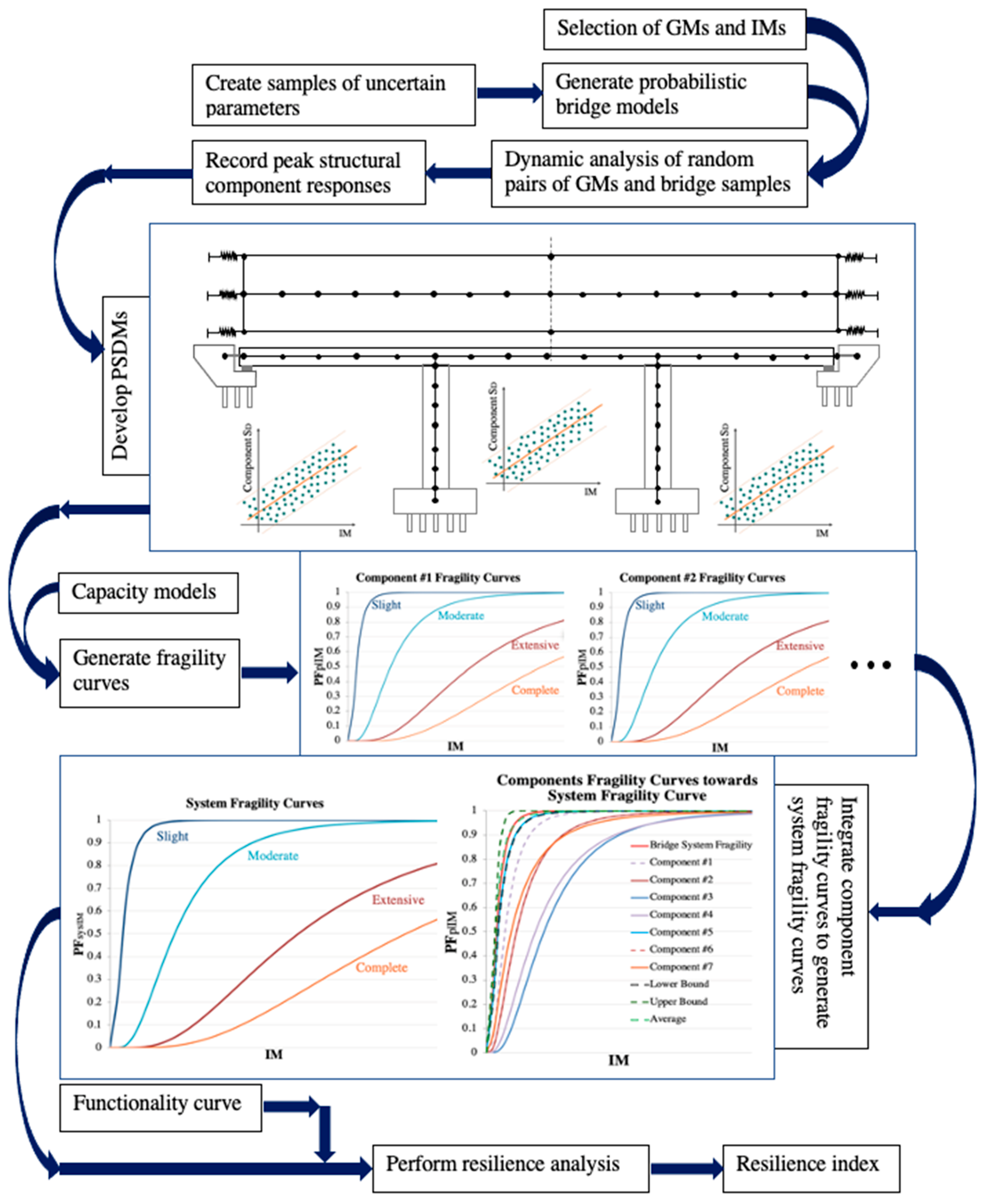
3.1. Fragility Curves

Fragility curves have emerged as essential tools in performance-based earthquake engineering to identify the potential seismic risk during an earthquake. Many researchers (e.g., [6,7,8,9,10,11,22,61,62]) have used PSDMs to generate analytical fragility curves to characterize the conditional reliability of the existing highway transportation network. Analytical fragility curves, initially introduced by Yu et al. [63], were further extended by Hwang, et al. [5], Gardoni, et al. [6], and Zhong, et al. [9]. Seismic fragility curves express the probability of exceeding predefined particular damage states under varying levels of earthquake intensity. These states are typically defined according to the extent of the damage ranging from slight to the collapsed state (e.g., slight, moderate, extensive, and complete) (FEMA, 2009).
The estimate of the bridge system fragility curve is performed through the development of a joint probabilistic seismic demand model, using the correlation between the demands of the various bridge components, in conjunction with Monte Carlo simulations [7]. The upper conservative bound on the system fragility assumes no correlation between the component demands (Equation (22)), while the lower unconservative bound assumes a complete correlation.
max p P F p | I M P F s y s t e m | I M 1 p [ 1 P F p | I M ]
Along with the assumption of log-normally distributed seismic capacity ( S C ), the probability of seismic demand ( S D ) exceeding capacity can be written as the following normal cumulative function (i.e., Φ ( . ) ), for the pth bridge component:
P F p | I M = P [ S D S C | I M ] = Φ ( ln ( μ D M S C ) β D M 2 + β C 2 )
Recently, alternative approaches such as parameterized and surrogated models (e.g., representative studies are [17,64,65,66]), which are primarily based on logistic regression and incorporate various input parameters in the regression model, have been proposed to estimate this probability. Discussion of this probability calculation and potential methods are beyond the scope of this study due to limited space, while interested readers can refer to the review article by Muntasir Billah and Shahria Alam [67] for more details on developments on fragility analysis procedures.

3.2. Resilience

The literature on seismic resilience assessment of bridges is not as expansive as fragility models. This is primarily due to the lack of a consensus definition of resilience and its more complicated procedure. In recent years, resilience and its means of quantification have received particular attention in the engineering community [68]. Given the multidisciplinary and interchangeable nature of the resilience concept, it has often been confused with other concepts such as vulnerability, reliability, and risk.
Woods [69] described resilience around four basic concepts: ’1. Resilience as a rebound from trauma and return to equilibrium; 2. Resilience as a synonym for robustness; 3. resilience as the opposite of brittleness; and 4. Resilience as a network architecture that can sustain the ability to adapt to future surprises as conditions evolve’. Most resilience quantification techniques reported in the literature are aligned with the first definition where resilience is defined as a function of quantifiable and time-dependent system performance indicator/delivery function/figure-of-merit. System performance indicator, often represented by Q ( t ) , defines the functionality of the system. Henry and Ramirez-Marquez [70] used a trapezoid function to describe system behavior in response to a disruptive event and corresponding recovery stage. The area underneath the trapezoid function is then divided by five zones, as shown in Figure 5: Zone 1: represents the status quo equilibrium zone; Zone 2: represents the failure absorption zone; Zone3: is the initiation of recovery; Zone 4: represents the recovery zone; and Zone 5: shows post-recovery equilibrium zone. Hajializadeh and Imani [71] have expanded the trapezoid description to cover different failure absorption and recovery/restoration trajectories for different assets. Both failure absorption and recovery/restoration trajectory functions can be represented by different trajectories/patterns, as shown by shaded areas in Figure 5. The resilience can be then quantified as either the area of loss of functionality (negative connotation) or as the area of remaining functionality (positive connotation), also referred to as the resilience triangle/trapezoid.
Most literature in the field of seismic resilience assessment (also known as lifecycle assessment) expresses resilience as follows:
R ( t ) = t 0 t Q ( t ) d t t t 0
where Q ( t ) represents the system/structure performance/functionality with time, t 0 , the start time and/or time of seismic event occurrence, and t represents investigation time horizon. Sharma [72] proposed additional metrics for quantifying resilience using probability theory analogy: resilience density function, cumulative resilience function, resilience disparity, center of resilience, median of resilience, mode of resilience, resilience bandwidth, and resilience moment. The study presented the mathematical approach in deriving these metrics as a function of the rate of recovery progress, also referred to as the resilience density function.
The performance indicator/functionality Q ( t ) of a bridge is another debatable and versatile component of seismic resilience assessment. This is often described by establishing the relationship between bridge damage level and the associated loss of functionality [19]. To account for the associated uncertainties in these relationships, Decò et al. [73] proposed a probabilistic approach. The studies conducted by Jia et al. [74] and Sharma et al. [75] defined the performance function as instantaneous reliability. For this purpose, the four damage levels of ATC-38 [76] were described in terms of the reliability of the structure, delimited by means of three thresholds. Briaud et al. [77] provided details of specifying these thresholds as a function of the system.
The relationship between the damage level and the corresponding loss of functionality defines the level of performance drop in Zone 2. To the best of authors’ knowledge, the literature in the field of seismic resilience assessment simplifies the failure absorption function as a sudden drop in performance indicator with no consideration of failure absorption time or failure absorption pattern. This assumption is not too unrealistic as a failure because a seismic event is often instantaneous and/or the failure absorption time can be negligible in comparison to the recovery/restoration process (Zone 3–4). FEMA [78] and Decò et al. [73] used fragility curves to provide the probability of the bridge being in a certain damage state and used damage states defined in ATC [79] to quantify the residual functionality associated with the bridge damage level defined. A similar concept has been used in the study by Karamlou and Bocchini [80]. In their study, the authors described functionality as reduced traffic-carrying capacity with a sudden drop in capacity upon the occurrence of a seismic event and defined the expected functionality of the structure at time t as:
Q ¯ ( t ) = s = 1 n I M P ( I M = s ) d = 1 n D S P ( D S = d | I M = s ) Q d ( t )
where P ( I M = s ) is the probability of occurrence of an extreme event with an intensity of I M = s , driven from a typical probabilistic seismic hazard analysis; and P ( D S = d | I M = s ) is the conditional probability of occurrence of damage level d given the event intensity of I M = s , driven from the fragility curve. Q d ( t ) is the functionality recovery function given damage level d . In their study, the recovery functions of ATC-13 [79] are adapted to formulate Q d ( t ) . The literature shows that the efforts in quantifying resilience have been predominantly focused on recovery/restoration trajectories/functions (Zone 4). Gidaris et al. [81] presented an overview of these restoration functions. In general, the proposed bridge seismic recovery/restoration models are grouped into two categories: 1. Probabilistic analytical models; 2. Models driven from expert judgment. One of the versatile theoretical models for recovery is Bocchini et al.’s restoration trajectory, expressed as [82]:
Q ( t > t 0 + δ i ) = Q r + H ( t t 0 δ i ) R s ( t t 0 δ i δ r ) ( Q t Q r )
where t 0 represents the time of occurrence of the seismic event; Q r is the residual functionality upon the occurrence of the event; H ( · ) is the Heaviside step function; Q t is the functionality after completion of the recovery process; δ r is the duration of recovery; δ i is the time lag between the occurrence of the seismic event and the beginning of the recovery, also referred as recovery initiation time; and R s ( · ) is the restoration function. This is one of few studies that considered the time lag between full failure absorption and initiation of recovery. In Bocchini et al.’s study [82], a six-parameter sinusoidal function was considered for R s ( · ) , which captures a variety of restoration from linear [83,84] to trigonometric [85] to exponential [86].
The largest challenge in analytical models is their calibration as it depends on a variety of parameters such as case-specific preparedness and resources for recovery and restoration, logistics, and prioritization strategy. To address this challenge, several studies used expert knowledge to derive recovery and restoration models. Among common models is HAZUS-MH [87], which defined restoration/recovery as a normal cumulative distribution function with the mean and standard deviation of m t , d and σ t , d , respectively. The subscript d and t represent different damage states and time, respectively. This formulation does not consider the versatility of recovery functions as a function of bridge type. This model has been used in several studies to quantify resilience, e.g., [80,88,89]. A similar approach was proposed by Padgett and DesRoches [19] using the CSUS Department of Transportation’s bridge inspectors’ and officials’ opinions. The model was used in the study conducted by [90] to optimize the bridge retrofit program post-earthquake. The basis of ATC [79] recovery functions is also expert opinions that provide the mean time required to reach 30%, 60%, and 100% of the normal functionality of the structure and assuming structure has lost its full 100% capacity. Table 3 provides a summary of studies that have utilized a form of PSDMs to generate fragility curves and assessed the resilience of bridges under seismic hazards. The search strategy for this table covers important studies that have used a form of PDSMs and/or fragility analysis and subsequently have quantified bridge resilience as a function of fragility. In all studies reviewed, the failure propagation pattern is a sudden drop in performance with varying thresholds for each damage state. Apart from the fragility functions’ form, the studies also differ in recovery trajectories. Among the five studies considered, three have quantified resilience as a function of PGA only. This is used to investigate the correlation of the resilience metric versus the fragility curve used to describe the vulnerability of the bridges studied. Figure 6 shows the correlation coefficients for all three studies and for different levels of damage state. The difference in patterns relates to the magnitude of the drop in functionality (i.e., residual functionality), fragility curve parameters, PSDMs model, the assumption on bridge age and its aging behavior, and recovery trajectory functions.

4. Discussion

4.1. Comparative Analysis of Highlighted Methodologies

Despite the extensive works on improving the demand models in a variety of directions, the simplest univariate demand model called the conventional model above (see Section 2.1: Description of PSDM and Univariate Linear Model), is yet commonly used in practice. In fact, the simplest form of the conventional model makes its application convenient. However, it may over- or underestimate the seismic demands of bridge components and consequently the vulnerability of the structure. Furthermore, a number of uncertainties are not quantified explicitly in the response function and the predictions may be biased for a particular range of ground motions. Additionally, none of the existing attempts toward developing PSDMs proposed a generalizable model that could replace the conventional model.
The established ML-based demand models provide a basis for considering various uncertainties for the analytical measurement of seismic demands, but their application is still very limited. Although according to the reviewed articles machine learning seems to be a promising approach to enhance the estimation of demands, the research on improving bridge PSDMs is still growing and yet some challenges need to be addressed in future studies. The applied ML methods possess their advantages, inherent drawbacks, and challenges for practical applications. To elucidate the link across available literature, the key advantages and disadvantages of the commonly proposed approaches are presented in Table 4. This information indicates that despite advances in the analytical demand models, there remains scope for significant improvement.
As described earlier in Section 2 (see Table 1 and Table 2), most of the efforts in this topic proposed models with the focus on regional risk assessments. Since different regions have different bridge types and specifications such as seismicity, design guidelines, and construction practices, the models generated are structure-specific and may not yet be extended to the other bridge types or similar bridges with different material properties, geometry, and location. Furthermore, different studies adopted different modeling and analysis approaches that have been adopted for certain structural types and configurations with specific detailing. Moreover, inconsistency is observed among the studies in this domain in terms of modeling and analysis approaches along with different assumptions to simplify the procedures and the considered uncertain parameters. All these factors render the limitations and lack of generality of developed PSDMs which restrict their applications in seismic performance evaluation of bridges.
Valuable efforts have been made to extend the generalization capability of the demand models. To this end, most studies considered representative bridges with significant variations in the structural parameters to produce demand models of a portfolio of bridges. These models involve multiple predictors to reflect the variation across the considered portfolio. A vast majority of these models incorporate many input variables; this is beneficial in the aspect of including various sources of uncertainty, but in terms of the performance of predictive models, adding many variables could lead to overfitting data and misinterpretation of the estimated demands.
The applied ML methods computational effort by developing predictive demand models to replace the numerical simulations. The literature proved that the general linear models, specifically when having embedded feature selection techniques, with multiple predictors provide a reliable estimate of the seismic demands. Particularly, this method allows the consideration of various uncertain parameters such as geometric, material, aging, and soil properties by expanding the number of input variables in the model. This method suffers from several drawbacks, such as the low prediction power to capture nonlinearity, prior assumption on the log-normality distribution of the demands, and the required specific number of excitations to achieve an acceptable performance. Specifically, the assignment of the prior distribution, while it is often unknown and may not be compatible for all bridge classes, poses subjective bias on the prediction model. Furthermore, in the case of the polynomial response models, the computational time rises drastically with the increasing number of input variables. Moreover, the prediction errors are assumed to fit a normal distribution. To compensate for these drawbacks, other methods such as decision trees are proposed. To overcome the potential overfitting problem associated with a single decision tree, ensemble learning approaches such as random forest implements bagging and aggregating strategies to combine multiple trees. Despite being computationally expensive, random forest outperforms the other methods for predicting the seismic demands of bridge components. Although this method is easily interpretable, the future application of its black-box model is complicated since it does not generate a formulation for the predictive demand model. Similarly, neural network methods indicated great potential in accurately predicting the bridge demands while being able to provide prediction formulation and manage data scarcity without overfitting data.
Overall, the existing PSDMs presented in this paper can be improved in many directions. According to the reviewed literature, we summarize a list of remarks on the current needs and challenges in the existing models, and potential future directions are provided next.

4.2. Challenges to Be Addressed in Future Research

This section highlights the grand challenges and provides recommendations for potential future research advancement to enhance the capability of PSDMs. Particularly, considering these points establish the path for the community to generate credible and practical PSDMs toward more reliable decision-making for the seismic performance assessment of bridges. The remarks follow:
  • The primary reason for the popularity of the univariate conventional model is its simplicity. However, the growing advanced statistical and ML methodologies make it feasible to develop efficient yet simple PSDMs with the most influential set of predictors that would be practical to infer. Despite the existing variety of ML algorithms, there is a gap between all the theoretical aspects and the engineering applications related to the PSDMs. Although there has been a growing body of research to implement the recently developed ML methodologies, such methods have not yet been widely applied in PSDMs, and more studies are needed to apply novel ML approaches on various bridge types. Their application in seismic resilience assessment is also yet to be explored.
  • The log-normality assumption of the demand and capacity needs to be reassessed. As mentioned in the previous sections, a couple of more recent studies proved that this assumption is not compatible with all demands and bridge types. The distribution type can lead researchers to choose the appropriate ML algorithm since every algorithm has its own underlying assumptions for the input and output distribution.
  • Generally, a PSDM model correlates selective input parameters to a specific demand parameter. Although some of the proposed response surface models provide higher accuracy, using too many predictors, on one hand, increases the chance of overfitting and on the other hand, makes the final model impractical to implement in practice. To this end, the design of the experiment or a prior sensitivity analysis was commonly performed to consider specific input parameters in each round of analyses. In fact, this issue can be currently addressed effortlessly as a part of developing the model, using the capabilities of ML approaches such as the feature selecting techniques (such as elastic net, stepwise regression, LASSO, and random forest) that are embedded in the model-training algorithms. These techniques have been used by a few researchers for basic models, but they should be considered as an essential step to integrate with more complex models such as PRSM.
  • As mentioned earlier (see section titled Description of PSDM and Univariate Linear Model), the selection of appropriate IMs is critical for developing a practical PSDM. However, in the conventional form of PSDM (i.e., Equations (2) and (3)), a single IM is chosen to estimate demands. A variety of IMs exists that their level of importance as an input variable in the PSDM needs to be assessed. This can lead to PSDMs with multiparameter IM to include parameters such as the PGA, PGV, etc. As stated earlier, some studies proposed an optimal intensity measure for specific bridge types by iteratively varying IMs in the models while monitoring the resulting variations in the estimated demand. However, these findings may not be generalized to bridges with different characteristics since each study is limited to a particular bridge type and specific structural parameters. For example, spectral acceleration could be a suitable candidate for bridge components whose response is significantly correlated with Sa. This typically happens when the corresponding response has not yet reached a highly inelastic range, and its seismic demand is governed by a single fundamental mode of vibration. On the contrary, alternative IMs need to be investigated to take the effect of inelasticity and the higher modes of vibration. There yet remains a principal milestone to identify the IMs that are highly correlated with the demands of various components of a bridge and to propose a more generalized recommendation for the selection of efficient IMs in developing PSDMs.
  • Previous studies investigated PSDMs for a variety of EDPs (commonly selected arbitrarily or based on engineering judgment) among which the demands associated with the bridge column failure are found to be the most common primary demand in estimating the vulnerability of the bridge system. In order to incorporate the results of PSDMs into the fragility and resilience evaluation of bridges, the PSDMs of the various bridge components need to be derived individually; then, individual fragilities are generated for each component, and these fragilities are combined in a later step to determining the fragility of the bridge system. In this process, the correlation between the EDPs is often assumed, as noted in previous literature. However, this correlation could alter the overall conclusions. Thereby, further research is required to investigate the influence of this correlation on the fragility and resilience analysis. Moreover, the correlation between the responses of the different bridge components can be analyzed using advanced ML approaches to improve the overall assessment. Moreover, there is a potential to incorporate all EDPs of interest into a single multivariate PSDM. In fact, such a model could not only replace the costly derivation of the system’s fragility from individual fragilities but would also be able to capture the correlation between different EDPs.
  • Overall, for the prediction of bridge demands, the application of tree-based ML algorithms and the polynomial orders higher than two and nonlinear methods is limited. Previous studies found decision tree and ANN algorithms effective in terms of capturing the complexity in data. Among the available tree-based methods, only random forest has been tested by a few researchers; hence, future research can investigate the performance of other bagging and boosting algorithms such as least squares boosting. Furthermore, it was noted that the application of ANN in this field is very limited. In this ML approach, the number of hidden layers and the number of nodes influence the efficiency of the ANN algorithm [94]. As stated, previous studies that applied ANN only used one hidden layer and assumed a particular number of nodes for their analysis. However, on the application of ANN for estimating the bridge S D , further studies are needed to determine the optimal number of hidden layers as well as the number of nodes to optimize the model efficiency.
  • As described, PSDMs are extensively used to generate analytical fragility curves that are used to estimate the resilience of bridges. To this end, relatively few studies have focused on applying different ML algorithms to improve fragility functions. In particular, most studies parameterized fragility functions that are primarily developed through logistic regression. Thus, research needs to explore the performance of other methods in terms of fragility analysis of bridges.
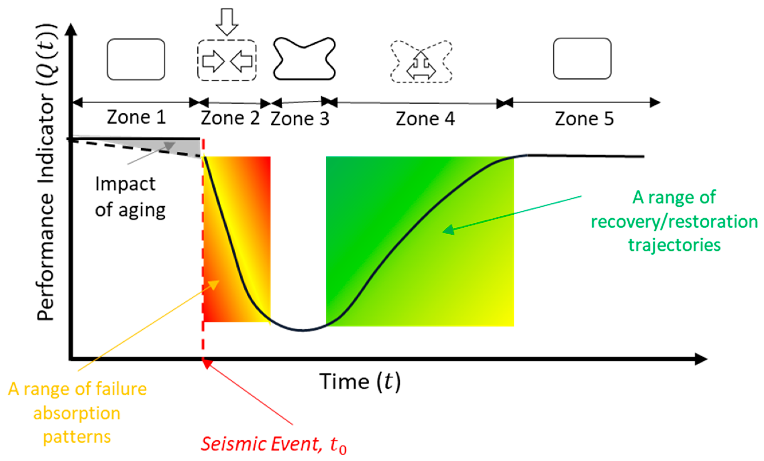
  • Similar to the fragility analysis, the relevant studies on the resilience assessment of bridges need to be expanded. As it is shown in the Resilience section, there is no clear consensus in resilience and lifecycle assessment using PSDMs. The literature is in agreement that the failure absorption patterns upon seismic event occurrence can be simplified as a sudden drop in functionality/performance with an associated probability of exceedance. However, the main difference in approaches seems to be focused on formulating the recovery trajectories. While many have proposed a variety of analytical trajectories to account for different scenarios, some have simplified the recovery/restoration patterns as a sudden rise in functionality with mean recovery time, driven by expert judgment.

4.3. Potential Future Developments

Given the advancements in technologies and computational techniques that lead to the growth of diverse data, ML approaches have a tremendous potential to revolutionize predictions in natural hazard engineering. Despite the growing body of research, the implementation of ML in improving the probabilistic seismic analysis of bridges is in its early stages. Research advances in this domain can be further expanded to leverage the efficiency and advantages that ML methods offer. To this end, this section presents potential future opportunities toward the future growth of ML application in evaluating bridges subjected to seismic hazards.
For developing ML-based PSDMs, different researchers used different suites of ground motions and training data as each study focused on a specific portfolio of bridges. Using a common standard data structure makes the proposed models more comparable and the findings more generalizable. In this regard, establishing a widely acceptable, community-driven platform such as DesignSafe is beneficial for researchers to store, share, and integrate large-scale training data for the future ML application, and also for practicing the tested ML algorithms.
Previous studies proved the importance of the selection of ground motions on the accuracy of derived demand models and the reliability of fragility curves. Therefore, as an initial step, it is critical to creating a suitable, accessible set of ground motions such as the NGA motion database. Moreover, there is a need for further investigation of the optimal number of ground motions and selection of an appropriate IM to develop a reliable model, since there is yet a topic of debate among researchers.
Although several ML algorithms have been implemented to propose improved PSDMs, state-of-the-art still falls short on providing a comprehensive comparative analysis of different methods and identifying the optimal or most suitable approach. To this end, a research study, such as the work by Soleimani [95], is required to focus on a systematic investigation of various ML algorithms in which a well-constructed framework needs to be followed for training, validating, and testing the models. An additional separate procedure for testing the model’s performance on a different dataset or using either case-history data or sensor-based recordings can significantly improve the generalization capability of the models.
Testing the efficiency and accuracy of the PSDMs is essential to find the appropriate model. There are three common evaluation criteria, as described in this section, to assess the performance of predictive models. Although a single criterion can be used, as found in most of the reviewed literature, the assessment performance in which all three criteria are evaluated is recommended for future studies to increase the credibility of the proposed model.
One of these criteria is the root mean squared error (RMSE), global goodness-of-fit measure, which is computed based on Equation (27). Another criterion is R 2 that is also calculated using MSE, as denoted in Equation (28) in which σ 2 is the variance of the response in the original dataset. The other criterion is the relative maximum absolute error (RMAE) that measures the local fitness of a model, as calculated in Equation (29).
R M S E = M S E = i = 1 n ( S D i S ^ D i ) 2 n
R 2 = 1 M S E σ 2
R M A E = max i | S D i S ^ D i | σ 2
Moreover, k-fold cross-validation (CV) is recommended to be applied in the future as a well-known unbiased approach to evaluating the overall performance of an ML-based model that is particularly beneficial in the training–validation process to optimize the hyperparameters. This approach partitions data into random k* subsets that train the model based on (k*−1) subsets and keeps the remaining subset for validation. This process is repeated, and the error measures are averaged over the k-folds.
ANN algorithms have been proven to be efficient ML approaches to solve a vast variety of problems in many disciplines. ANN can outperform other ML methods while overcoming their limitations owing to its capability to capture the high-dimensional nonlinear relationship between the predictors and the EDPs. In this regard, the determination of the optimal network architecture, optimizing the associated solvers, and tuning the hyperparameters that play significant roles in the overall performance of the model needs a thorough investigation in future research, such as the research performed by Soleimani and Liu [96]. Furthermore, future studies on developing new PSDMs can extend the application of classic ANN to a deep neural network to boost the model performance, particularly when managing intricate patterns and scarcity in data or an ill-posed problem. Moreover, simplifying the network complexity can be a potential research topic. To this end, the most informative nodes in the network can be identified and an equivalent network can be constructed with only the most influential nodes without sacrificing the accuracy of the original network.
Another great contribution can be creating a single transparent and robust framework to predict the seismic demands of bridges by integrating advanced approaches. For example, the ANN algorithm can be combined with other artificial intelligence algorithms such as Bayesian updating to facilitate sensitivity analysis of demands to perturbation of parameters, providing confidence bounds, identifying correlated predictors, and handling incomplete datasets. Such an integrated framework provides a promising resource to create a transparent model that can simply be carried out in routine practice. In this framework, identifying the most plausible uncertain parameters in the model is an essential task to prevent or alleviate data overfitting issues. In addition, incorporating modification factors for specific bridge configurations will allow the changes to be easily adopted in the models.
Although researchers reported that the estimated seismic demand values of bridge components significantly depend on the proposed predictive model, implemented algorithms, and associated uncertain parameters, the impact of different model types is still unclear on the overall probabilistic seismic analysis. To this end, it is essential to explore to what extent the fragility and resilience of bridge systems are sensitive to the various seismic demand models and the applied ML algorithms [97].
Eventually, in addition to probe unexplored or less explored ML algorithms, there exists an emerging trend that requires researchers to develop new theory-guided ML algorithms for our application needs considering the physics-based characteristics of seismic demands of bridges.

5. Conclusions

Over recent years, extensive research has been performed to improve the efficiency of the probabilistic seismic demand models (PSDMs) of bridges. Nonetheless, the findings from these studies may not be generalized since each is limited to a specific bridge type, a particular relationship between the IMs and the demand, assumptions on the distribution of the demands, certain analysis methodologies, and also limited in terms of the number of applied excitations, and arbitrarily selected list of demands and IMs. As a result, the conventional simplest form of PSDM that expresses the seismic demand of interest in terms of the ground motion intensity measure continues to be used in practice.
Natural hazard engineering is benefiting from well-established machine-learning (ML) approaches. Although ML implementation is a high-impact research area in earthquake engineering, it is in its rising stages to reliably predict seismic demands of highway bridges. This state-of-the-art review presents the significance of various ML algorithms implemented for improving probabilistic seismic demand models. This article reveals that ML algorithms have potential promise to learn complex interrelations among contributing parameters in estimating the seismic demands, to handle various sources of uncertainty, and to manage large-scale problems having diverse data structures.
Moreover, this study presents a state-of-the-art review of the existing PSDMs with ML application to broaden insight into these models, to increase the usability of the current models, and to extend the research for enhancing the PSDMs. The overview and general conclusions shed light on a way to select an appropriate PSDM based on matching the specifications of a problem and the model attributes provided in this study. The application of proposed PSDMs in fragility analysis and their incorporation into the resilience assessment are also described. Furthermore, according to the overview of the existing models, this study highlights the challenges and current needs to be addressed by future research to facilitate the practical application of the PSDMs. This article can serve as a reference for researchers to encourage and guide broader advances in ML application, providing a more reliable risk assessment tool for highway bridges to ensure the reliability of transport facilities. Since this study is limited to bridges, future studies should explore the efficiency of alternative PSDMs for the seismic demand modeling of other structural systems.

Author Contributions

The authors declare that they have both made substantial contributions to the conception or design of the work, drafted the work for important intellectual content, approved the version to be published, and agree to be accountable for all aspects of the work in ensuring that questions related to the accuracy or integrity of any part of the work are appropriately investigated and resolved. All authors have read and agreed to the published version of the manuscript.

Funding

This research received no external funding.

Institutional Review Board Statement

Not applicable.

Informed Consent Statement

Not applicable.

Data Availability Statement

Not applicable.

Conflicts of Interest

The authors declare no conflict of interest.

References

  1. Ang, A.-S.; De Leon, D. Modeling and analysis of uncertainties for risk-informed decisions in infrastructures engineering. Struct. Infrastruct. Eng. 2005, 1, 19–31. [Google Scholar] [CrossRef]
  2. Mackie, K.; Stojadinovic, B. Probabilistic Seismic Demand Model for California Highway Bridges. J. Bridge Eng. 2001, 6, 468–481. [Google Scholar] [CrossRef] [Green Version]
  3. Shome, N.; Cornell, C.A.; Bazzurro, P.; Carballo, J.E. Earthquakes, Records, and Nonlinear Responses. Earthq. Spectra 1998, 14, 469–500. [Google Scholar] [CrossRef]
  4. Cornell, C.A.; Krawinkler, H. Progress and challenges in seismic performance assessment. PEER CTR News 2000, 3, 1–3. [Google Scholar]
  5. Hwang, H.; Jernigan, B.J.; Lin, W.Y. Evaluation of seismic damage to Memphis bridges and highway systems. J. Bridge Eng. 2000, 5, 322–330. [Google Scholar] [CrossRef]
  6. Gardoni, P.; Mosalam, K.M.; DER Kiureghian, A. Probabilistic seismic demand models and fragility estimates for RC bridges. J. Earthq. Eng. 2003, 7, 79–106. [Google Scholar] [CrossRef]
  7. Nielson, B.G. Analytical Fragility Curves for Highway Bridges in Moderate Seismic Zones. Doctoral Dissertation, Georgia Institute of Technology, Atlanta, GA, USA, 2005. [Google Scholar]
  8. Padgett, J.E.; DesRoches, R. Methodology for the development of analytical fragility curves for retrofitted bridges. Earthq. Eng. Struct. Dyn. 2008, 37, 1157–1174. [Google Scholar] [CrossRef]
  9. Zhong, J.; Gardoni, P.; Rosowsky, D.; Haukaas, T. Probabilistic Seismic Demand Models and Fragility Estimates for Reinforced Concrete Bridges with Two-Column Bents. J. Eng. Mech. 2008, 134, 495–504. [Google Scholar] [CrossRef]
  10. Ramanathan, K.N. Next Generation Seismic Fragility Curves for California Bridges Incorporating the Evolution in Seismic Design Philosophy. Doctoral Dissertation, Georgia Institute of Technology, Atlanta, GA, USA, 2012. [Google Scholar]
  11. Soleimani, F. Fragility of California Bridges-Development of Modification Factors. Doctoral Dissertation, Georgia Institute of Technology, Atlanta, GA, USA, 2017. [Google Scholar]
  12. Freddi, F.; Padgett, J.E.; Dall’Asta, A. Probabilistic seismic demand modeling of local level response parameters of an RC frame. Bull. Earthq. Eng. 2017, 15, 1–23. [Google Scholar] [CrossRef]
  13. Ma, H.-B.; Zhuo, W.-D.; Lavorato, D.; Nuti, C.; Fiorentino, G.; Marano, G.C.; Greco, R.; Briseghella, B. Probabilistic seismic response and uncertainty analysis of continuous bridges under near-fault ground motions. Front. Struct. Civ. Eng. 2019, 13, 1510–1519. [Google Scholar] [CrossRef]
  14. Maleki, S. Deck modeling for seismic analysis of skewed slab-girder bridges. Eng. Struct. 2002, 24, 1315–1326. [Google Scholar] [CrossRef]
  15. Shamsabadi, A.; Rollins, K.M.; Kapuskar, M. Nonlinear soil–abutment–bridge structure interaction for seismic performance-based design. J. Geotech. Geoenviron. Eng. 2007, 133, 707–720. [Google Scholar] [CrossRef]
  16. Monteiro, R.; Delgado, R.; Pinho, R. Probabilistic Seismic Assessment of RC Bridges: Part I—Uncertainty Models. In Structures; Elsevier: Amsterdam, The Netherlands, 2016; Volume 5, pp. 258–273. [Google Scholar]
  17. Xie, Y.; Zhang, J.; Desroches, R.; Padgett, J.E. Seismic fragilities of single-column highway bridges with rocking column-footing. Earthq. Eng. Struct. Dyn. 2019, 48, 843–864. [Google Scholar] [CrossRef]
  18. Xie, Y.; DesRoches, R. Sensitivity of seismic demands and fragility estimates of a typical California highway bridge to uncertainties in its soil-structure interaction modeling. Eng. Struct. 2019, 189, 605–617. [Google Scholar] [CrossRef]
  19. Padgett, J.E.; Desroches, R. Sensitivity of Seismic Response and Fragility to Parameter Uncertainty. J. Struct. Eng. 2007, 133, 1710–1718. [Google Scholar] [CrossRef] [Green Version]
  20. Soleimani, F.; Vidakovic, B.; DesRoches, R.; Padgett, J. Identification of the significant uncertain parameters in the seismic response of irregular bridges. Eng. Struct. 2017, 141, 356–372. [Google Scholar] [CrossRef]
  21. Soleimani, F.; Mangalathu, S.; DesRoches, R. A comparative analytical study on the fragility assessment of box-girder bridges with various column shapes. Eng. Struct. 2017, 153, 460–478. [Google Scholar] [CrossRef]
  22. Mangalathu Sivasubramanian Pillai, S. Performance Based Grouping and Fragility Analysis of Box-Girder Bridges in California. Doctoral Dissertation, Georgia Institute of Technology, Atlanta, GA, USA, 2017. [Google Scholar]
  23. Huang, Q.; Gardoni, P.; Hurlebaus, S. Probabilistic Seismic Demand Models and Fragility Estimates for Reinforced Concrete Highway Bridges with One Single-Column Bent. J. Eng. Mech. 2010, 136, 1340–1353. [Google Scholar] [CrossRef]
  24. Bin Ma, H.; Zhuo, W.D.; Yin, G.; Sun, Y.; Chen, L.B. A Probabilistic Seismic Demand Model for Regular Highway Bridges. Appl. Mech. Mater. 2016, 847, 307–318. [Google Scholar] [CrossRef]
  25. Seo, J.; Linzell, D.G. Use of response surface metamodels to generate system level fragilities for existing curved steel bridges. Eng. Struct. 2013, 52, 642–653. [Google Scholar] [CrossRef]
  26. Ghosh, J.; Padgett, J.E.; Dueñas-Osorio, L. Surrogate modeling and failure surface visualization for efficient seismic vulnerability assessment of highway bridges. Probab. Eng. Mech. 2013, 34, 189–199. [Google Scholar] [CrossRef]
  27. Pan, Y.; Agrawal, A.K.; Ghosn, M. Seismic Fragility of Continuous Steel Highway Bridges in New York State. J. Bridg. Eng. 2007, 12, 689–699. [Google Scholar] [CrossRef]
  28. Seo, J.; Linzell, D.G. Probabilistic Vulnerability Scenarios for Horizontally Curved Steel I-Girder Bridges under Earthquake Loads. Transp. Res. Rec. J. Transp. Res. Board 2010, 2202, 206–211. [Google Scholar] [CrossRef]
  29. Seo, J.; Linzell, D.G. Horizontally curved steel bridge seismic vulnerability assessment. Eng. Struct. 2012, 34, 21–32. [Google Scholar] [CrossRef]
  30. Park, J.; Towashiraporn, P. Rapid seismic damage assessment of railway bridges using the response-surface statistical model. Struct. Saf. 2014, 47, 1–12. [Google Scholar] [CrossRef]
  31. Seo, J.; Park, H. Probabilistic seismic restoration cost estimation for transportation infrastructure portfolios with an emphasis on curved steel I-girder bridges. Struct. Saf. 2017, 65, 27–34. [Google Scholar] [CrossRef]
  32. Du, A.; Padgett, J.E.; Shafieezadeh, A. Adaptive IMs for improved seismic demand modeling of highway bridge portfolios. In Proceedings of the 11th National Conference in Earthquake Engineering, Los Angeles, CA, USA, 25–29 June 2018. [Google Scholar]
  33. Mangalathu, S.; Jeon, J. Stripe-based fragility analysis of multispan concrete bridge classes using machine learning techniques. Earthq. Eng. Struct. Dyn. 2019, 48, 1238–1255. [Google Scholar] [CrossRef]
  34. Soleimani, F. Analytical seismic performance and sensitivity evaluation of bridges based on random decision forest framework. Structures 2021, 32, 329–341. [Google Scholar] [CrossRef]
  35. Pang, Y.; Dang, X.; Yuan, W. An Artificial Neural Network Based Method for Seismic Fragility Analysis of Highway Bridges. Adv. Struct. Eng. 2014, 17, 413–428. [Google Scholar] [CrossRef]
  36. Mangalathu, S.; Heo, G.; Jeon, J.-S. Artificial neural network based multi-dimensional fragility development of skewed concrete bridge classes. Eng. Struct. 2018, 162, 166–176. [Google Scholar] [CrossRef]
  37. Kameshwar, S.; Padgett, J.E. Response and fragility assessment of bridge columns subjected to barge-bridge collision and scour. Eng. Struct. 2018, 168, 308–319. [Google Scholar] [CrossRef]
  38. Kameshwar, S.; Padgett, J.E. Multi-hazard risk assessment of highway bridges subjected to earthquake and hurricane hazards. Eng. Struct. 2014, 78, 154–166. [Google Scholar] [CrossRef]
  39. Du, A.; Padgett, J.E. Multivariate surrogate demand modeling of highway bridge structures. In Proceedings of the 12th Canadian Conference on Earthquake Engineering, Quebec City, QC, Canada, 17–20 June 2019; pp. 17–20. [Google Scholar]
  40. Choe, D.-E.; Gardoni, P.; Rosowsky, D.; Haukaas, T. Seismic fragility estimates for reinforced concrete bridges subject to corrosion. Struct. Saf. 2009, 31, 275–283. [Google Scholar] [CrossRef]
  41. Zhong, J.; Gardoni, P.; Rosowsky, D. Bayesian Updating of Seismic Demand Models and Fragility Estimates for Reinforced Concrete Bridges with Two-Column Bents. J. Earthq. Eng. 2009, 13, 716–735. [Google Scholar] [CrossRef]
  42. Zakeri, B.; Padgett, J.E.; Amiri, G.G. Fragility Analysis of Skewed Single-Frame Concrete Box-Girder Bridges. J. Perform. Constr. Facil. 2014, 28, 571–582. [Google Scholar] [CrossRef]
  43. Tondini, N.; Stojadinovic, B. Probabilistic seismic demand model for curved reinforced concrete bridges. Bull. Earthq. Eng. 2012, 10, 1455–1479. [Google Scholar] [CrossRef]
  44. Soleimani, F.; Yang, C.S.W.; DesRoches, R. The Effect of Superstructure Curvature on the Seismic Performance of Box-Girder Bridges with In-Span Hinges. In Structures Congress; American Society of Civil Engineers: Reston, VA, USA, 2017; pp. 469–480. [Google Scholar]
  45. Abbasi, M.; Zakeri, B.; Amiri, G.G. Probabilistic Seismic Assessment of Multiframe Concrete Box-Girder Bridges with Unequal-Height Piers. J. Perform. Constr. Facil. 2016, 30, 04015016. [Google Scholar] [CrossRef]
  46. Noori, H.Z.; Amiri, G.G.; Nekooei, M.; Zakeri, B. Seismic Fragility Assessment of Skewed MSSS-I Girder Concrete Bridges with Unequal Height Columns. J. Earthq. Tsunami 2016, 10, 1550013. [Google Scholar] [CrossRef] [Green Version]
  47. Soleimani, F. Propagation and quantification of uncertainty in the vulnerability estimation of tall concrete bridges. Eng. Struct. 2020, 202, 109812. [Google Scholar] [CrossRef]
  48. Johnson, R.A.; Wichern, D.W. Applied Multivariate Statistical Analysis, 5th ed.; Prentice-Hall: Englewood Cliffs, NJ, USA, 2002. [Google Scholar]
  49. James, G.; Witten, D.; Hastie, T.; Tibshirani, R. An Introduction to Statistical Learning; Springer: New York, NY, USA, 2013. [Google Scholar]
  50. Miller, A. Subset Selection in Regression; CRC Press: Boca Raton, FL, USA, 2002. [Google Scholar]
  51. Tibshirani, R. Regression Shrinkage and Selection via the Lasso: A retrospective. J. R. Stat. Soc. 2011, 73, 267–288. [Google Scholar] [CrossRef]
  52. Shafieezadeh, A.; Ramanathan, K.; Padgett, J.E.; DesRoches, R. Fractional order intensity measures for probabilistic seismic demand modeling applied to highway bridges. Earthq. Eng. Struct. Dyn. 2012, 41, 391–409. [Google Scholar] [CrossRef]
  53. Ho, T.K. The random subspace method for constructing decision forests. IEEE Trans. Pattern Anal. Mach. Intell. 1998, 20, 832–844. [Google Scholar] [CrossRef] [Green Version]
  54. Heidari, A.A.; Faris, H.; Aljarah, I.; Mirjalili, S. An efficient hybrid multilayer perceptron neural network with grasshopper optimization. Soft Comput. 2019, 23, 7941–7958. [Google Scholar] [CrossRef]
  55. Huang, D.-S. Radial basis probabilistic neural networks: Model and application. Int. J. Pattern Recognit. Artif. Intell. 1999, 13, 1083–1101. [Google Scholar] [CrossRef]
  56. Bugmann, G. Normalized Gaussian Radial Basis Function networks. Neurocomputing 1998, 20, 97–110. [Google Scholar] [CrossRef]
  57. Jin, R.; Chen, W.; Simpson, T. Comparative studies of metamodelling techniques under multiple modelling criteria. Struct. Multidiscip. Optim. 2001, 23, 1–13. [Google Scholar] [CrossRef]
  58. Friedman, J.H. Multivariate adaptive regression splines. Ann. Stat. 1991, 19, 1–67. [Google Scholar] [CrossRef]
  59. Jekabsons, G.; Zhang, Y. Adaptive basis function construction: An approach for adaptive building of sparse polynomial regression models. Mach. Learn. 2010, 1, 127–155. [Google Scholar]
  60. Rosipal, R.; Krämer, N. Overview and Recent Advances in Partial Least Squares. In International Statistical and Optimization Perspectives Workshop “Subspace, Latent Structure and Feature Selection”; SLSFS 2005; Lecture Notes in Computer Science; Springer: Berlin/Heidelberg, Germany, 2006; Volume 3940, pp. 34–51. [Google Scholar]
  61. Jeong, S.-H.; Elnashai, A.S. Probabilistic fragility analysis parameterized by fundamental response quantities. Eng. Struct. 2007, 29, 1238–1251. [Google Scholar] [CrossRef]
  62. Mangalathu, S.; Soleimani, F.; Jeon, J.-S. Bridge classes for regional seismic risk assessment: Improving HAZUS models. Eng. Struct. 2017, 148, 755–766. [Google Scholar] [CrossRef]
  63. Yu, O.; Allen, D.L.; Drnevich, V.P. Seismic vulnerability assessment of bridges on earthquake priority routes in Western Kentucky. In Lifeline Earthquake Engineering; ASCE: Reston, VA, USA, 1991; pp. 817–826. [Google Scholar]
  64. Sichani, M.E.; Padgett, J.E.; Bisadi, V. Probabilistic seismic analysis of concrete dry cask structures. Struct. Saf. 2018, 73, 87–98. [Google Scholar] [CrossRef]
  65. Jeon, J.-S.; Mangalathu, S.; Song, J.; Desroches, R. Parameterized Seismic Fragility Curves for Curved Multi-frame Concrete Box-Girder Bridges Using Bayesian Parameter Estimation. J. Earthq. Eng. 2017, 23, 954–979. [Google Scholar] [CrossRef]
  66. Balomenos, G.P.; Kameshwar, S.; Padgett, J.E. Parameterized fragility models for multi-bridge classes subjected to hurricane loads. Eng. Struct. 2020, 208, 110213. [Google Scholar] [CrossRef]
  67. Muntasir Billah, A.H.M.; Shahria Alam, M. Seismic fragility assessment of highway bridges: A state-of-the-art review. Struct. Infrastruct. Eng. 2015, 11, 804–832. [Google Scholar] [CrossRef]
  68. Hosseini, S.; Barker, K.; Ramirez-Marquez, J.E. A review of definitions and measures of system resilience. Reliab. Eng. Syst. Saf. 2016, 145, 47–61. [Google Scholar] [CrossRef]
  69. Woods, D.D. Four concepts for resilience and the implications for the future of resilience engineering. Reliab. Eng. Syst. Saf. 2015, 141, 5–9. [Google Scholar] [CrossRef]
  70. Henry, D.; Ramirez-Marquez, J.E. Generic metrics and quantitative approaches for system resilience as a function of time. Reliab. Eng. Syst. Saf. 2012, 99, 114–122. [Google Scholar] [CrossRef]
  71. Hajializadeh, D.; Imani, M. RV-DSS: Towards a resilience and vulnerability-informed decision support system framework for interdependent infrastructure systems. Comput. Ind. Eng. 2021, 156, 107276. [Google Scholar] [CrossRef]
  72. Sharma, N.; Tabandeh, A.; Gardoni, P. Resilience analysis: A mathematical formulation to model resilience of engineering systems. Sustain. Resilient Infrastruct. 2018, 3, 49–67. [Google Scholar] [CrossRef] [Green Version]
  73. Decò, A.; Bocchini, P.; Frangopol, D.M. A probabilistic approach for the prediction of seismic resilience of bridges. Earthq. Eng. Struct. Dyn. 2013, 42, 1469–1487. [Google Scholar] [CrossRef]
  74. Jia, G.; Tabandeh, A.; Gardoni, P. Life-Cycle Analysis of Engineering Systems: Modeling Deterioration, Instantaneous Reliability, and Resilience. In Risk and Reliability Analysis: Theory and Applications; Springer International Publishing: Cham, Switzerland, 2017; pp. 465–494. [Google Scholar]
  75. Sharma, N.; Tabandeh, A.; Gardoni, P. Regional resilience analysis: A multiscale approach to optimize the resilience of interdependent infrastructure. Comput. Civ. Infrastruct. Eng. 2020, 35, 1315–1330. [Google Scholar] [CrossRef]
  76. Applied Technology Council (ATC). Database on the Performance of Structures Near Strong-Motion Recordings: 1994 Northridge, California, Earthquake; Rep. No. ATC-38; Applied Technology Council: Redwood City, CA, USA, 2000. [Google Scholar]
  77. Briaud, J.-L.; Gardoni, P.; Yao, C. Statistical, Risk, and Reliability Analyses of Bridge Scour. J. Geotechnol. Geoenviron. Eng. 2014, 140, 04013011. [Google Scholar] [CrossRef]
  78. FEMA. HAZUS-MH MR4–Earthquake Model User Manual; FEMA: Washington, DC, USA, 2009. [Google Scholar]
  79. Applied Technology Council (ATC). Earthquake Damage Evaluation Data for California; Applied Technology Council: Redwood City, CA, USA, 1985. [Google Scholar]
  80. Karamlou, A.; Bocchini, P. Computation of bridge seismic fragility by large-scale simulation for probabilistic resilience analysis. Earthq. Eng. Struct. Dyn. 2015, 44, 1959–1978. [Google Scholar] [CrossRef]
  81. Gidaris, I.; Padgett, J.E.; Barbosa, A.; Chen, S.; Cox, D.; Webb, B.; Cerato, A. Multiple-Hazard Fragility and Restoration Models of Highway Bridges for Regional Risk and Resilience Assessment in the United States: State-of-the-Art Review. J. Struct. Eng. 2017, 143, 04016188. [Google Scholar] [CrossRef]
  82. Bocchini, P.; Decò, A.; Frangopol, D. Probabilistic functionality recovery model for resilience analysis. In Proceedings of the Bridge Maintenance, Safety, Management, Resilience and Sustainability, Stresa, Italy, 8–12 July 2012; pp. 1920–1927. [Google Scholar]
  83. Bocchini, P.; Frangopol, D.M. Optimal Resilience- and Cost-Based Postdisaster Intervention Prioritization for Bridges along a Highway Segment. J. Bridge Eng. 2012, 17, 117–129. [Google Scholar] [CrossRef]
  84. Chandrasekaran, S.; Banerjee, S. Retrofit Optimization for Resilience Enhancement of Bridges under Multihazard Scenario. J. Struct. Eng. 2016, 142, 4015012. [Google Scholar] [CrossRef]
  85. Cimellaro, G.P.; Reinhorn, A.M.; Bruneau, M. Seismic resilience of a hospital system. Struct. Infrastruct. Eng. 2010, 6, 127–144. [Google Scholar] [CrossRef]
  86. Kafali, C.; Grigoriu, M. Rehabilitation decision analysis. In ICOSSAR’05: Proceedings of the Ninth International Conference on Structural Safety and Reliability; IOS Press: Amsterdam, The Netherlands, 2005. [Google Scholar]
  87. Hazus, M.H. Multi-Hazard Loss Estimation Methodology: Earthquake Model Hazus-MH MR5 Technical Manual; FEMA: Washington, DC, USA, 2011. [Google Scholar]
  88. Zhou, Y.; Banerjee, S.; Shinozuka, M. Socio-economic effect of seismic retrofit of bridges for highway transportation networks: A pilot study. Struct. Infrastruct. Eng. 2010, 6, 145–157. [Google Scholar] [CrossRef]
  89. Venkittaraman, A.; Banerjee, S. Enhancing resilience of highway bridges through seismic retrofit. Earthq. Eng. Struct. Dyn. 2014, 43, 1173–1191. [Google Scholar] [CrossRef]
  90. Chang, L.; Peng, F.; Ouyang, Y.; Elnashai, A.S.; Spencer, B.F., Jr. Bridge seismic retrofit program planning to maximize postearthquake transportation network capacity. J. Infrastruct. Syst. 2012, 18, 75–88. [Google Scholar] [CrossRef]
  91. Pang, Y.; Wei, K.; Yuan, W. Life-cycle seismic resilience assessment of highway bridges with fiber-reinforced concrete piers in the corrosive environment. Eng. Struct. 2020, 222, 111120. [Google Scholar] [CrossRef]
  92. Fu, Z.; Gao, R.; Li, Y. Probabilistic Seismic Resilience-Based Cost–Benefit Analysis for Bridge Retrofit Assessment. Arab. J. Sci. Eng. 2020, 45, 8457–8474. [Google Scholar] [CrossRef]
  93. Vishwanath, B.S.; Banerjee, S. Life-Cycle Resilience of Aging Bridges under Earthquakes. J. Bridge Eng. 2019, 24, 04019106. [Google Scholar] [CrossRef]
  94. Rafiq, M.; Bugmann, G.; Easterbrook, D. Neural network design for engineering applications. Comput. Struct. 2001, 79, 1541–1552. [Google Scholar] [CrossRef]
  95. Soleimani, F. Probabilistic seismic analysis of bridges through machine learning approaches. Structures 2022, 38, 157–167. [Google Scholar] [CrossRef]
  96. Soleimani, F.; Liu, X. Artificial neural network application in predicting probabilistic seismic demands of bridge components. Earthq. Eng. Struct. Dyn. 2021, 51, 612–629. [Google Scholar] [CrossRef]
  97. Soleimani, F.; Hajializadeh, D. Bridge seismic hazard resilience assessment with ensemble machine learning. Structures 2022, 38, 719–732. [Google Scholar] [CrossRef]
Figure 1. Illustration of the general framework for the probabilistic seismic analysis of bridges.
Infrastructures 07 00064 g001
Figure 2. Temporal and spatial distribution of the initial literature search: (a) temporal distribution and (b) spatial distribution. (Adopted from Scopus—note that the spatial distribution only covers countries with more than 2% share of the total number of publications).
Infrastructures 07 00064 g002
Figure 3. Schematic illustration of the univariate PSDM in log–log space.
Infrastructures 07 00064 g003
Figure 4. Layout for multilayer artificial neural network to estimate seismic demand.
Infrastructures 07 00064 g004
Figure 5. Schematic demonstration of system performance indicator in response to a failure event.
Infrastructures 07 00064 g005
Figure 6. Correlation coefficient of resilience metric and fragility curves.
Infrastructures 07 00064 g006
Table 1. Summary of main contributions to propose alternative PSDMs for bridges.
StudyBridge Demand ParametersIntensity
Measure
Investigated Input Uncertain
Variables in the Formulation
Bridge TypeMethodology
Huang, Q., Gardoni, P., and Hurlebaus, S., 2010 [23]Seismic univariate deformation and shear, bivariate deformation–shear demandsPseudo-spectral acceleration and peak ground velocity12 parameters including span length, column height, column diameter-to-superstructure depth ratio, reinforcement nominal yield strength, concrete nominal strength, longitudinal reinforcement ratio, transverse reinforcement ratio, degree of skew, bridge dead load, pile soil stiffness, abutment models, two-span ratioReinforced concrete highway bridge with single-column bent and two spansCorrection term as a set of explanatory functions;
using Bayesian updating approach
Ma, H.B., Zhuo, W.D., Yin, G., Sun, Y., and Chen, L.B., 2016 [24]Maximum drift ratio at top of piersThe spectral acceleration at the fundamental period with 5% dampingOne parameter: fundamental period (T)Single column, regular continuous concrete highway bridges with three spans in China—8 representative regular highway bridgesMultiplicative factor as a function of fundamental period
Soleimani, 2017 [11]Column curvature ductility, abutment displacementSpectral acceleration at 1.0 sOne parameter corresponding to a geometric irregularity such as skew angle, tall column height, and unbalanced frame stiffness ratioBox-girder concrete bridges in CaliforniaMathematical optimization techniques; Levenberg–Marquardt method; Bayesian updating
Xie, Y., Zhang, J., DesRoches, R., and Padgett, J. E., 2019 [17]Uplift demand (column drift ratio and normalized uplift angle)Peak ground velocity, frequency duration, cumulative absolute velocity of exceedance, frequency at the largest spectral velocityRocking frequency parameter, effective heightSingle-column concrete box-girder bridge with rocking isolation in CaliforniaGeneral linear model with stepwise regression
Soleimani, F., Vidakovic, B., DesRoches, R., and Padgett, J. E., 2017 [20]Column curvature ductility, foundation rotation and displacement, displacement of deck, abutment, bearing, and shear keySpectral acceleration at 1.0 s42 categorical and numerical parameters including modeling, structural, material, and geometric characteristics of bridgesConcrete box-girder bridges in California with: (i) skew angle, (ii) a frame with unbalanced stiffness, and (iii) tall column heightsGeneral linear model with LASSO
Xie, Y. and DesRoches, R., 2019 [18]Column displacement ductility, displacements of abutment, foundation, bearing, and shear keySpectral acceleration at 1.0 s18 random variables corresponding to soil-structure interaction that cover different soil zonesA two-span prestressed concrete box-girder bridge in California and supported on diaphragm abutments and a two-column central bentGeneral linear model with stepwise regression and LASSO
Seo and Linzell, 2013 [25]Peak radial bearing deformations, peak tangential bearing deformations, peak radial abutment deformations directly adjacent to the bearing seats, peak tangential abutment deformations directly adjacent to the bearing seats, column curvature ductilityPeak ground acceleration13 macrolevel and microlevel parameters;
number of spans, maximum span length, deck width, maximum column height, radius of curvature, girder spacing, cross-frame spacing, damping ratio, compressive and tensile strength and Young’s modulus of concrete, steel reinforced modulus and yield strength
Horizontally curved steel I-girder bridges in Pennsylvania, New York, and Maryland2nd order polynomial response surface model
Ghosh, J., Padgett, J.E., and Dueñas-Osorio, L., 2013 [26]Column curvature ductility, longitudinal and transverse deformations of bearings and abutmentSpectral acceleration at the geometric mean of periods in the longitudinal and transverse directions10 parameters including steel strength, elastomeric bearing pad friction and gap and bar area, column reinforcing bar area, shear modulus of elastomeric bearing pads, concrete cover depth, column height, midspan length, number of columns per bentMultispan (three-span three columns per bent) simply supported concrete girder bridge2nd order polynomial response surface model, multivariate adaptive regression splines, radial basis function networks, and support vector machines
Pan, Y., Agrawal, A.K., and Ghosn, M., 2007 [27]Pier curvature, high and low type rocker bearing displacementPeak ground acceleration, moment magnitude, and epicentral distanceNot availableContinuous multispan I-girder steel highway bridge in New YorkGeneral linear model and 2nd order polynomial response surface model
Seo and Linzell, 2010, 2012 [28,29]Peak radial bearing deformations, peak tangential bearing deformations, peak radial abutment deformations directly adjacent to the bearing seats, peak tangential abutment deformations directly adjacent to the bearing seats, column curvature ductilityPeak ground accelerationNumber of spans, maximum span length, radius of curvature, girder spacing, cross-frame spacingHorizontally curved steel I-girder bridges in Pennsylvania, New York, and Maryland2nd order polynomial response surface model
Park and Towashirapor, 2014 [30]Seismic damage of bearings, piers, and abutments in terms of the maximum value of a response, such as displacement or curvaturePeak ground accelerationPhysical configuration of the bridge including the number of spans, span length, and pier heightFive span steel-plate girder bridges in Korea2nd order polynomial response surface model
Seo and Park, 2017 [31]Peak responses corresponding to radial and tangential abutment components, radial and tangential bearing components, and pier columnsPeak ground accelerationNumber of spans, maximum span length, deck width, maximum column height, radius of curvature, girder spacing, cross-frame spacingCurved steel I-girder bridges in Eastern United States2nd order polynomial response surface model
Du, A., Padgett, J. E., and Shafieezadeh, A., 2018 [32]Column drift, displacement of expansion bearings and displacement of fixed bearingsOne parameter from spectral acceleration and geometric mean of spectral accelerations at several periods, a total of four one-parameter adaptive IMs and two fractional-order adaptive IMs16 structure-related parameters for concrete bridge class and 14 structure-related parameters for slab bridge classTwo case-study highway bridge classes (multispan simply supported concrete girder bridges and multispan continuous slab) in Central and Southeastern United States2nd order polynomial response surface model with stepwise regression
Mangalathu and Jeon, 2019 [33]Column curvature ductility, displacement of abutment and bearing, and superstructure unseatingSpectral acceleration at 1.0 s23 parameters including geometric, material, and structural modeling characteristicsThree four-span concrete box-girder bridges in CaliforniaRandom forest
Soleimani, 2021 [34]Column curvature ductility, displacement of deck, abutment, and bearingSpectral acceleration at 1.0 s24 parameters including geometric, material, and structural modeling characteristicsMultispan concrete box-girder bridges with tall piers within low, medium, and high column height ratiosRandom forest
Pang, Y., Dang, X., and Yuan, W., 2014 [35]Curvatures of cross sections of columns, displacements of bearings and abutmentsPeak ground acceleration16 selected material properties (four parameters for the confined concrete and three parameters for the unconfined concrete) and geometric parameters (span length, column height, deck width, column diameter, gap between girder and abutment and concrete cover)Three-span continuous bridge with two columns per bent in ChinaMultilayer radial basis function neural networks
Mangalathu, S., Heo, G., and Jeon, J.S., 2018 [36]Curvature ductility of column, maximum displacement of abutments, maximum deformation of bearing, maximum unseating deformation of superstructureSpectral acceleration at 1.0 s23 parameters including categorical variables (e.g., the number of columns per bent, backfill type), numerical variables (e.g., the number of spans, the number of columns), and continuous variables (e.g., span length, concrete compressive strength)Two-, three-, and four-span skewed concrete box-girder bridge with single and two columns per bent and seat abutmentArtificial neural networks with sigmoid activation function (one hidden layer with 10 neurons)
Kameshwar and Padgett, 2018 [37]Shear and moment demands on bridge columnsPeak ground acceleration32 parameters design and geometric parameters related to superstructure, column, and sub-structure elements together with soil parameters and the barge collision conditionsSimply supported bridges (with six simply supported spans) on navigable waterways with large circular, elliptical, or wall type columns supported on pile foundations4th order polynomial response surface model with stepwise regression
Kameshwar and Padgett, 2014 [38]Peak column curvature ductility, abutment and bearing displacementsPeak ground accelerationConcrete nominal strength, reinforcement yield strength, span length, column height and diameter, width of deck, number of spans, longitudinal and transverse reinforcement ratiosMultispan simply supported concrete girder bridges located in South CarolinaPolynomial response surface models with three orders, adaptive basis function construction, multivariate adaptive regressive splines, and radial basis function interpolation
Du and Padgett, 2019 [39]Column drift ratio, longitudinal and transverse deformation of expansion bearings and fixed bearings, abutment deformationsSpectral acceleration at the geometric mean of periods in the longitudinal and transverse directions14 parameters for concrete bridges
16 parameters for steel bridges
Two case studies: simply supported concrete girder and continuous steel girder bridge typeMultivariate linear regression, linear and partial kernel 2nd and 3rd order (L-PLSR and K-PLSR), artificial neural networks with a single hidden layer
Table 2. Key aspects of the sample studies reviewed in this article.
StudyKey AspectsApplicability Case Studies
Gardoni, P., Mosalam, K.M., and Der Kiureghian, A., 2003 [6]; Choe, D. E., Gardoni, P., Rosowsky, D., and Haukaas, T., 2009 [40]; Zhong, J., Gardoni, P., and Rosowsky, D., 2009 [41]; Huang, Q., Gardoni, P., and Hurlebaus, S., 2010 [23]Produced probabilistic model from deterministic; moderate bias; improve accuracyGeneral type of bridges
Ma, H.B., Zhuo, W.D., Yin, G., Sun, Y., and Chen, L.B., 2016 [24]Proposed simplified empirical expression for drift ratio of the bridge columnsGeneral type of bridges
Soleimani, 2017 [11]Proposed modified PSDMs to derive EDPs of irregular bridges; stiffness frames of bridgesIrregular bridges including skew angle, tall piers, and unbalanced stiffness frames of bridges.
Xie, Y., Zhang, J., DesRoches, R., and Padgett, J.E., 2019 [17]Accounted for rocking isolation parameters; estimated full contact damage, rocking, and overturning probability of the bridge columnGeneral type of bridges
Soleimani, F., Vidakovic, B., DesRoches, R., and Padgett, J.E., 2017 [20]Identified influential uncertain parameters for bridges with geometric irregularitiesBridges with geometric irregularities
Xie and Desroches, 2019 [18]Investigated the sensitivity of seismic demands to variation in its soil-structure interaction (SSI) modeling parametersTypical highway bridge
Seo and Linzell, 2013 [25];
Seo and Linzell, 2010 [28];
Seo and Linzell, 2012 [29]
Examined the influence of important parameters on their seismic responseHorizontally curved steel I-girder
Gosh, J., Padgett, J.E., and Dueñas-Osorio, L., 2013 [26]Explored four different metamodeling strategies to predict bridge responsesGeneral type of bridges
Pan Y., Agrawal, A.K., and Ghosn, M., 2007 [27]Performed an analytical seismic fragility analysis along with sensitivity assessment if seismic response to variations in superstructure mass, gap size, concrete compressive strength, reinforcing bar yield stress, friction coefficient of expansion bearing, and abutment wall–soil stiffnessTypical steel highway bridge
Park and Towashiraporn, 2014 [30]Used response surface model to median and variation in seismic damageSteel-plate-girder bridges
Du, A., Padgett, J.E., and Shafieezadeh, A., 2018 [32]Established systematic optimization process to adaptively identify the optimal IM parameters to characterize the correlation between IMs and structural responsesGeneral type of bridges
Seo and Park, 2017 [31]Generated restoration curvesPortfolio of regional curved I-girder bridges
Mangalathu and Jeon, 2019 [33]Generated bridge-specific fragility curves using random forestGeneral type of bridges
Soleimani, 2021 [34]Conducted sensitivity analysis of seismic demandsBridges with tall piers
Pang, Y., Dang, X., and Yuan, W., 2014 [35]Proposed an artificial neural network-based prediction scheme to replace the extremely time-consuming process in traditional analytical fragility methodologiesGeneral type of bridges
Mangalathu, S., Heo, G., and Jeon, J.S., 2018 [36]Investigated the applicability of artificial neural network in the generation of seismic fragility curves for regional risk assessment of bridges to reduce computationally intensive procedureGeneral type of bridges
Kameshwar and Padgett, 2018 [37]Developed parameterized polynomial response surface models to predict the shear and flexural response for a wide range of bridge characteristics and collision conditions without model-based simulationGeneral type of bridges
Kameshwar and Padgett, 2014 [38]Generated parametric bridge fragility functions for bridges with different geometric and structural properties given exposure to different hazard typesGeneral type of bridges
Du and Padgett, 2019 [39]Provided a comparative study of four different multivariate surrogate demand modeling approachesGeneral type of bridges
Table 3. Summary of studies utilizing PSDMS and fragility curves for resilient assessment purposes.
StudyFragility ModelsResilience
Quantification
Technique
Recovery
Trajectory Profile
Correlation
Coefficient Range between Resilience and
Fragility Curves
Resilience as
Lifecycle Analysis
Resilience Metric Reporting System
Pang, Wei, and Yuan
(2020) [91]
Analytical fragility using PSDMs in Equations (3) and (4)Equation (24)Equation (26) with positive negative exponential, and trigonometric recovery profile[0.7–0.9]Resilience as a function of time of occurrence and peak ground acceleration
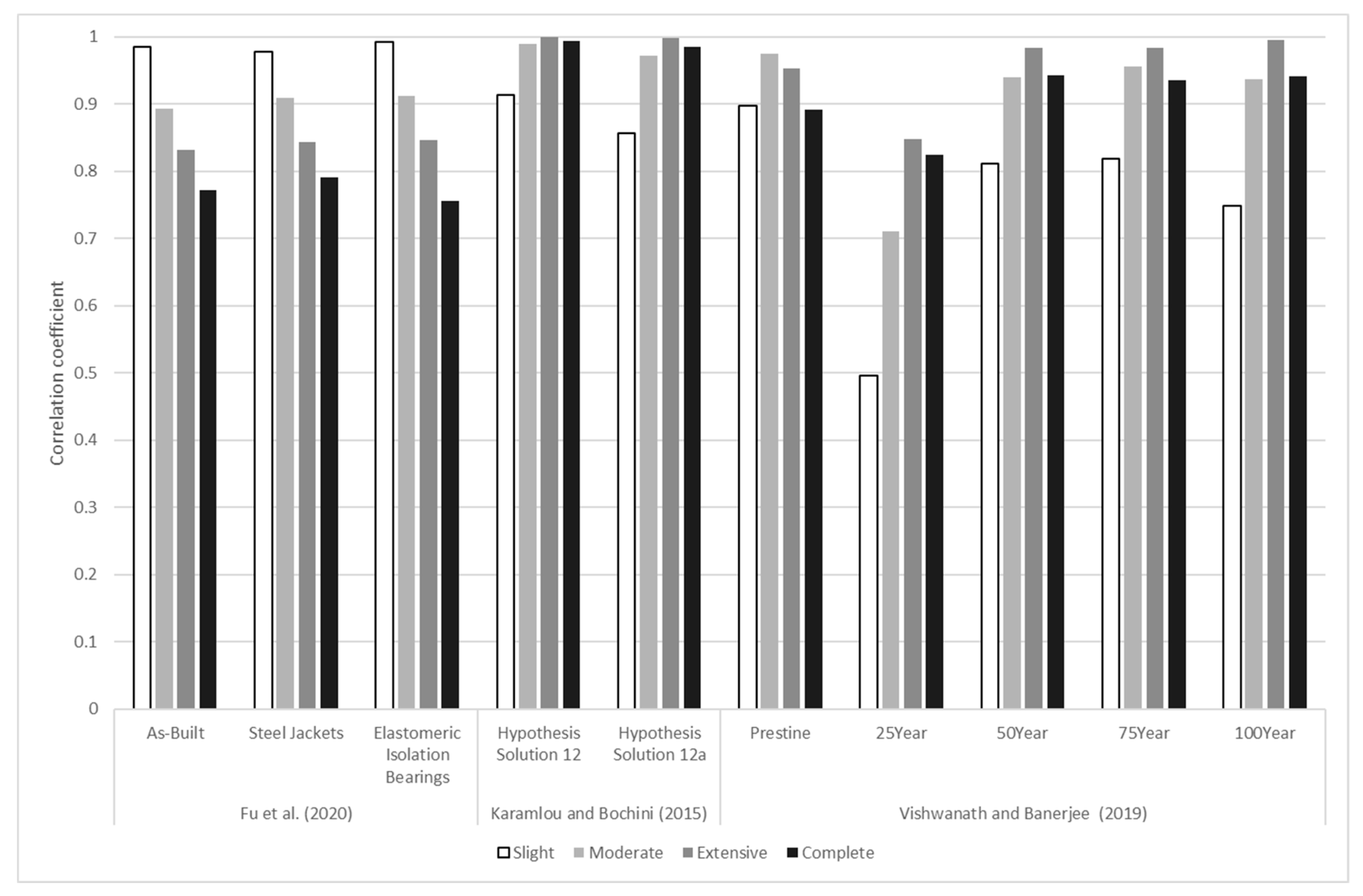
Fu, Gao, and Li (2020) [92]Analytical fragility using PSDMs in Equations (3) and (4)Equation (24) Q ( t ) = γ ( α ( t ) Q 1 ( t ) + β ( t ) Q 2 ( t ) )
And Equation (26) to define Q 1 ( t ) and Q 2 ( t ) and using experimental data for constant parameters
[0.77–0.98]Resilience as a function of peak ground acceleration
Karamlou and Bocchini (2015) [80]Analytical fragility using PSDMs in Equations (3) and (4)Equation (24)ATC-13[0.85–0.99]Resilience as a function of peak ground acceleration
Venkittaraman and Banerjee (2014) [89]Simulation-based analytical fragility without using PSDMsEquation (24)Linear, negative exponential, and trigonometricN/A resilience is not reported as a function of PGAResilience as a function of recovery or control time
Vishwanath and Banerjee (2019) [93]Simulation-based analytical fragility without using PSDMsEquation (24)Equation (26) and sigmoidal recovery profile[0.49–0.99]Resilience as a function of age and peak ground acceleration
Table 4. Comparison of the main approaches of proposed methods for development of probabilistic seismic demand models of bridges.
MethodFundamental AdvantagesFeatured Disadvantages/Drawbacks
Unidimensional linear regression
-
Simple model
-
Easy to implement
-
Based upon log-normality assumption
-
Only one input parameter for different components of a bridge and different classes of bridges
-
Does not take into account uncertain variables other than an IM in the regression model
Modification factors
-
Easily generate PSDMs of bridges with particular characteristics using the already developed PSDMs for typical bridges
-
Can replace finite element modeling and NLTHA for specific bridge types
-
Covers specific bridge types
-
Accounts for restricted uncertain parameters
-
Modification factors need to be developed for a variety of bridges
-
Factors need to be optimized on a comprehensive dataset that leads to costly computations
-
Based upon log-normality assumption
Multiparameter general linear regression models, stepwise regression, LASSO
-
Considers different sources of uncertainty
-
Can replace complex and time-consuming models.
-
Low computational cost for stepwise regression.
-
LASSO is an efficient approach that assigns zero coefficients for redundant parameters
-
General models, without feature selection, have overfitting and complexity issue due to large number of input variables
-
Stepwise regression does not check all combinations of input variables hence it does not provide the best set of input variables
-
LASSO chooses the maximum number of variables to reach the best fit
Polynomial regression
-
Considers different sources of uncertainty
-
Can replace complex and time-consuming models.
-
Provide a better fit to data with no apparent linear correlation
-
Overfitted and complexity happens if feature selection techniques are not incorporated
-
Feature selection will be computationally expensive and sometimes infeasible particularly when interaction between variables is considered
-
Orders higher than 2 will produce complex models and have not been investigated yet
Random forest
-
Easy to interpret
-
Provide level of importance of uncertain parameters
-
Provide a great fit to a nonlinear dataset
-
No prior assumption on distribution of variables
-
Needs high computational power
-
Does not provide an actual formulation of the predictive model which makes it challenging for future application
-
Implementation might be difficult for future application without access to the source code
Artificial neural networks
-
Requires significantly less computational time compared to traditional approaches and other alternatives
-
Covers a wide range of relationships between the input and output variables
-
No prior assumption on distribution of variables
-
Many different algorithms exists so there is yet a need to find the most suitable algorithm for specific applications, demands, and bridge types
Publisher’s Note: MDPI stays neutral with regard to jurisdictional claims in published maps and institutional affiliations.

