Article

Automatic Recognition and Geolocation of Vertical Traffic Signs Based on Artificial Intelligence Using a Low-Cost Mapping Mobile System

Department of Cartographic and Terrain Engineering, Universidad de Salamanca, Calle Hornos Caleros 50, 05003 Ávila, Spain
*
Author to whom correspondence should be addressed.
Infrastructures 2022, 7(10), 133; https://doi.org/10.3390/infrastructures7100133
Submission received: 12 September 2022 / Revised: 27 September 2022 / Accepted: 30 September 2022 / Published: 4 October 2022

Abstract

:
Road maintenance is a key aspect of road safety and resilience. Traffic signs are an important asset of the road network, providing information that enhances safety and driver awareness. This paper presents a method for the recognition and geolocation of vertical traffic signs based on artificial intelligence and the use of a low-cost mobile mapping system. The approach developed includes three steps: First, traffic signals are detected and recognized from imagery using a deep learning architecture with YOLOV3 and ResNet-152. Next, LiDAR point clouds are used to provide metric capabilities and cartographic coordinates. Finally, a WebGIS viewer was developed based on Potree architecture to visualize the results. The experimental results were validated on a regional road in Avila (Spain) demonstrating that the proposed method obtains promising, accurate and reliable results.

1. Introduction

Among the different expenditure items that are part of the life cycle of transport infrastructure, maintenance is one of the most important. The development of transport infrastructure is a major investment for public administrations, and their life cycle can span decades. For that reason, proper maintenance is essential to get the best return on these investments [1]. However, according to data gathered by the European Road Federation (ERF), the volume of investment in inland transport infrastructure has stalled since a significant cut after the 2008 crisis, when it reached its maximum [2]. This is especially worrying considering that the transport of goods and passengers has been steadily growing for the last decade, and the infrastructure is ageing under a context of maintenance budget cuts. According to a study by Calvo-Poyo et al. [3], spending on road maintenance not only prevents deterioration and prolongs the life of the infrastructure, but also increases road safety, reducing the death rate.
The use of new technologies for capturing, managing, and communicating information is essential to optimize the cost of infrastructure maintenance and to increase its security and resilience. Transport infrastructure digitalization is a key concept that is supposed to drive the transition towards the goals of the Sustainable and Smart Mobility Strategy of the European Union [4].
Intelligent Transportation Systems (ITS) apply information and communication technologies to the infrastructure, vehicles and users, interfacing between different modes of transportation and potentially offering data management capabilities for road maintenance, and they are an intrinsic part of the future of transport [5]. Together with ITS, remote sensing technologies are being extensively reported in the literature for transportation infrastructure maintenance and assessment. While technologies such as satellites or aerial drones are used for specific applications such as road network mapping [6] or road traffic monitoring [7], they have several limitations when compared with Mobile Mapping Systems (MMS) in terms of versatility for carrying out different road network maintenance activities [8,9,10]. The main advantage of MMS in this context is the fact that they can be mounted on conventional vehicles, which drive around the infrastructure collecting data automatically, simplifying the field tasks of the operators, reducing their number and exposure to traffic, thus increasing their safety. The MMS are based on mapping technologies, mainly LiDAR and imagery (with laser scanners and cameras, respectively), providing 3D and 2D geometric and radiometric information of the environment, and global positioning technologies (Global Navigation Satellite System (GNSS)) that allow data geolocation. The literature has grown considerably during the last decade with applications of MMS for road infrastructure assessment, maintenance or inventory [11,12,13].
Among the different applications that can be carried out using MMS data, this work will focus on the inventory of vertical traffic signs. Their retro-reflective properties make them one of the most important visual elements when driving, especially at night. This is critically relevant in the context of traffic safety, as a large proportion of traffic fatalities occur at night [14], and the driver receives more than 90% of information visually [15]. Studies as the one in [16] show that the presence of traffic signalling and its correct layout improves driver behaviour, increasing traffic safety.
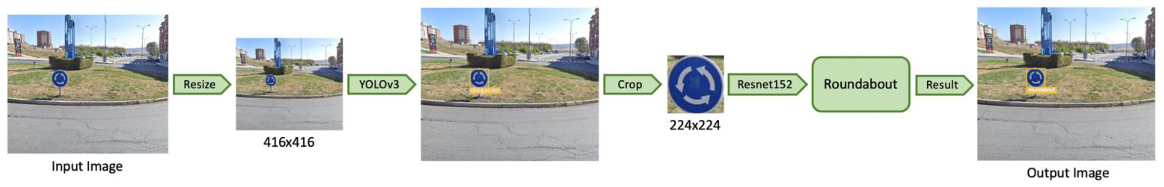
From the data collected by a MMS, the application of traffic sign inventory can have three different approaches, based on: (1) use of images, (2) use of point clouds, and (3) fusion of images and point clouds.
The image-based inventory of vertical traffic signs consists of the manual or automatic annotation of the signs present in images taken with cameras. In practice, the inventory process is still carried out manually or semi-automatically in many cases by maintenance companies, although the state of the art allows automatic processes with very good accuracies. This process can be divided into two parts: detection and recognition. Traffic sign detection involves the annotation of the position in the image coordinate system where the signs are located, while traffic sign recognition involves the assignment of semantics to the signs. In both cases, there are methods that allow an accurate resolution of these problems using architectures based on Deep Learning (DL). For the case of traffic sign detection, early approaches include the implementation of the AdaBoost based learning method and cascade structure [17], and the combination of handcrafted features such as the Histogram of Oriented Gradients (HOG) together with Machine Learning (ML) algorithms such as Support Vector Machines (SVM) [18], which were able to obtain almost perfect results in traffic sign recognition benchmarks, such as the German Traffic Sign Detection Benchmark (GTSDB) [19]. In recent years, many DL strategies have been developed based on Convolutional Neural Networks (CNN), showing state-of-the-art results [20,21]. The CNN-based architectures such as YOLOv3 [22], obtained remarkable results for real-time applications [23,24]. For traffic sign recognition, DL approaches have also a large presence in the literature. Arcos-García et al. [25] employed a combination of convolutional and spatial transformer [26] networks, and report a 99.71% accuracy at the German Traffic Sign Recognition Benchmark (GTSRB). Similar results have been achieved by large CNN ensembles together with data augmentation, as in [27].
Point cloud approaches have also been explored in the literature. The ability of MMS to capture the geometry of the environment and the radiometric properties of materials, provided a promising new research line for applications such as road asset inventory. Pu et al. [28] presented a methodology for structure recognition which, in the case of vertical signs, distinguished rectangular, circular and triangular shapes. Riveiro et al. [29] further developed this idea, making use of the intensity parameter of the point cloud to easily detect vertical traffic sign panels. It was concluded that, although the geometric shapes of the signs could be detected automatically, the resolution of the 3D information was not sufficient to provide the detected signs with semantic information.
Image-based and point cloud approaches have complementary advantages and disadvantages. While semantic recognition in images can be performed accurately with DL-based techniques, the geolocation of signals is not as straightforward as in the case of point cloud-based methods. Therefore, it seems logical to merge both sources of information to carry out inventory tasks. One possible approach is based on detecting signals in the point cloud from the geometric and radiometric properties of traffic signs, and projecting the 3D information onto images where recognition is performed using ML or DL approaches, given that the point cloud and the images are synchronized with each other [30,31]. Other works have a complementary workflow, performing both detection and recognition on the images, and projecting the result on the point cloud to geolocate the position of the road sign [8].
This paper presents a methodology for traffic signal inventory using MMS that follows the latter approach. First, the detection and recognition of traffic signs in images is carried out, and then the geolocation is performed on the point cloud, projecting the results obtained on the images. The contribution of this paper aims to close two gaps from previous works:
(1)
While previous works use high-end MMS (RIEGL VMX-450 in [30], Optech LYNX in [8,31]), which provide the calibration of their cameras and laser scanner system, this work uses a low-cost MMS with a commercial camera that was manually mounted together with the laser scanner. Thus, this methodology offers a complete workflow that includes the calibration between the camera and the laser scanner system to carry out the geolocation of traffic signs.
(2)
The 3D visualization of inventory results is a pending work in the literature. In this work, a 3D WebGIS based on Potree architecture [32] of large point cloud datasets is proposed.
This work is organized as follows. Section 2 will describe the case study data and the proposed methodology for traffic sign inventory. Section 3 will show and discuss the results obtained, focusing on the specific contributions that are being made. Finally, Section 4 will outline the conclusions and future directions of this work.

2. Materials and Methods

2.1. Case Study Data

The 3D point cloud data and 2D imagery for validation in this paper were acquired with a customized assembly of the Phoenix Scout Ultra 32 Mobile LiDAR System. It was a low-cost system equipped with a Velodyne VLP-32C laser scanner, that has a horizontal and vertical field of view of 360° and 40° respectively, and 32 laser beams. The scanner had a scan rate of 600,000 measurements per second and operated at a wavelength of 903 nm. The complete specifications of the scanner can be found in the reference [33]. The global positioning was solved with a single-antenna, dual-frequency RTK-GNNS receiver, whose position with respect to the laser and IMU was known and calibrated. A GNSS Topcon HiPer V, placed at less than 15 km from the trajectory, was used as a base for trajectory postprocessing with Inertial Explorer. A Sony A6000 camera was mounted manually, its position being fixed to that of the mobile mapping system. Due to the way the MMS was mounted on the vehicle and the need for calibration between the LiDAR and the camera, which requires the camera to point in the same direction as the LiDAR beams, the mounting of the camera was sub-optimal, pointing backwards and to the left with respect to the movement of the vehicle, hence offering a more challenging setup for traffic sign detection and recognition tasks (Figure 1a).
The case study consists of a point cloud and images acquired on a 6 km stretch of a regional road in the province of Ávila (Spain). The acquisition was performed in both directions, therefore the total trajectory was approximately 12 km (Figure 1b). The acquisition speed was adapted to the maximum speed limit of the road, which was 80 km/h. The point cloud contains approximately 222 million points. The image acquisition system was set to take one image every second, forming a dataset of 634 images.
Furthermore, a large image dataset was used to train the Deep Learning architectures employed in this work, with more than 56 thousand traffic sign images. The specific distribution of those images are outlined in Section 2.2.

2.2. Methodology

The methodological approach of this work can be conceptualized in two main blocks, as shown in Figure 2. The input data were the images and the 3D point cloud acquired by the MMS. The images were processed by a first block where DL architectures (YOLOv3 and ResNet152) were used to solve the detection and classification of traffic signs. This information, together with the calibration data from the camera and the LiDAR system, was used to extract the geographical position of the detected signs in the geolocation block. In this section, each of these blocks will be described in detail, as well as the calibration process of the camera and the LiDAR system.

2.2.1. Deep Learning Architecture

The Deep Learning part of the workflow consists of two different architectures: YOLOv3 and ResNet152. First, the input image is fed into the YOLOv3 network, which returns a new image in which traffic signs have been identified and classified into six different classes. This output image is then cropped into different images each containing an individual sign. Each of these images is used as an input to the ResNet152 architecture, which further classifies these signs into different subclasses (Figure 3).
YOLOv3 is a deep learning model used for object detection and classification [22]. This architecture uses Convolutional Neural Networks (CNNs) to provide object detection at three different scales that are then merged to produce the output (Figure 4). This output consists of a series of bounding boxes along with the recognized classes.
The ResNet152 architecture is a deep learning model used for image classification [34]. It consists of a Deep Residual Network of up to 152 convolutional layers. The residual network is constructed by adding identity connections between the layers, which adds information from the input of each layer to its output, allowing deeper networks to obtain state-of-the-art performance.
A large image dataset was used to train the Deep Learning architectures employed in this paper, with more than 56 thousand traffic sign images. Following the hierarchical classification schema, the YOLOv3 architecture was trained with 56,111 images, belonging to six traffic sign classes: Stop, yield, no entry, obligation, prohibition, and danger. For the case of obligation and prohibition, where a larger number of images were available, 27,308 images were used to train the ResNet152 architecture, to recognize 11 subclasses of prohibition signs, and 14 subclasses of obligation signs, as depicted in Figure 5. Training parameters are listed in Table 1.

2.2.2. Camera-LiDAR Calibration

The output data of the AI block consists of, on the one hand, images with bounding boxes corresponding to the signal detections, and, on the other hand, a text file including the path of each image together with a text string representing the classified signal, and the coordinates of its bounding box in the image coordinate system as a vector (x, y, w, h), where (x, y) are the pixel coordinates of the upper left corner of the bounding box and (w, h) are its width and height in pixel units.
This process alone is not sufficient for an accurate inventory of vertical signs, as the geographical location of the detected signs is not yet available at this stage. However, with the support of a 3D point cloud, this location can be obtained relatively easily if both 2D and 3D data are temporally and spatially synchronized.
The time synchronization is done from the GNSS of the MMS. Both the camera and the LiDAR store the Time of Week (TOW) from the GNSS: each image, and each point of the 3D point cloud have an associated timestamp, and both are synchronized with each other, so that it is possible to obtain point cloud data of a photographed scene given the time stamp of the acquisition of any image.
Spatial synchronization is more complex to implement. The objective is to know the geometric transformation needed to convert a three-dimensional coordinate in the point cloud to its corresponding two-dimensional coordinate in the image, and vice versa. Thus, it is important to define the coordinate systems that play a role in this step of the process (Figure 6):
  • Global coordinate system [ X w ,   Y w ,   Z w ] : A point P = ( x p ,   y p , z p ) in the 3D point cloud is measured in Universal Transverse Mercator (UTM) coordinates. That is, [ X w ,   Y w ] coordinates go North and East from an origin that depends on the UTM zone.
  • Vehicle coordinate system [ X v ,   Y v ,   Z v ] : It has its origin in the centre of navigation of the MMS, which coincides with the inertial measurement unit (IMU). The position and orientation of this system with respect to the global coordinate system is given in the vehicle trajectory file, with a frequency of 1 Hz (i.e., one point per second) corresponding to the GNSS, including for each point the 3D position and the three orientation angles (roll, pitch, and yaw) coming from the IMU.
  • Sensor co-ordinate system [ X s ,   Y s ,   Z s ] : It has its origin in the LiDAR sensor. The point cloud is initially registered in this coordinate system, and then transformed to the global coordinate system during its pre-processing. The transformation with respect to the vehicle coordinate system is given by the MMS calibration sheet.
  • Camera coordinate system [ X c ,   Y c ,   Z c ] : It defines the position of the optical centre and the orientation of the camera. As it was mounted on the vehicle without being initially related to the MMS, the transformation between this reference system and that of the sensor was unknown. Therefore, the spatial synchronization problem can be solved if this transformation is known, as well as the internal parameters of the camera.
For the calibration process of the transformation matrix between the sensor and camera coordinate systems ( T s c ), as well as for the calibration of the intrinsic parameters of the camera, a checkboard was used. It had 9 × 12 squares, and the side of each square measured 65 mm. The data collection for the calibration consisted of the simultaneous acquisition of images and point clouds from the checkboard. Nine pairs of point clouds and images were obtained for calibration (Figure 7).
First, the intrinsic parameters of the camera were calibrated using the images. All the parameters, including distortion coefficients, were estimated simultaneously using nonlinear least-squares minimization [35,36]. These parameters were internal and fixed to the camera employed, and they included:
  • Focal length, f. Distance between the optical centre of the camera (origin of the camera coordinate system) and the sensor along the optical axis.
  • Intrinsic matrix, M. Transformation between the 3D camera coordinates and the 2D image coordinates. Camera principal point ( c x , c y ) (intersection of the optical axis and the sensor) and focal length were embedded in this matrix (Equation (1)).
  • Coefficients for radial distortion ( k 1 , k 2 ) . They describe the lens distortion as a deviation from an ideal projection following the Gaussian model (Equation (2)), as a function of the distance r to the camera principal point.
    M = [ f 0 c x 0 f c y 0 0 0 ]
    x u = x u ( k 1 r 2 + k 2 r 2 ) ;   y u = y u ( k 1 r 2 + k 2 r 2 )
The results of this process, as well as the calibration error, will be shown and discussed in Section 3.2.
Then, the transformation matrix T s c was computed to perform LiDAR-camera data fusion. From a set of images and point clouds of the same scene it was possible to estimate the geometric relationship between the LiDAR and camera coordinate systems. For this purpose, the checkerboard was used. First, the checkerboard corners in the images and the checkerboard plane in the point cloud were extracted. Then, from a minimum of four image-point cloud pairs, this geometric information was used to obtain the transformation matrix T s c . The process is defined in detail in [37], and the results and calibration errors are shown in Section 3.2.

2.2.3. Geolocation and Inventory Visualization

The geolocation workflow for a single image with a traffic sign detected within the IA block is summarized in Figure 8. First, the input data is described:
  • Image: 2D image that contains a traffic sign, as detected by the IA block.
  • Bounding box: Vector ( x , y , w , h ) bb that contains the pixel coordinates of the upper-left corner, width, and height of the bounding box of the detected traffic sign.
  • Vehicle pose: Vector ( x , y , z ,   ϕ ,   θ ,   ψ ) v that contains the pose of the vehicle coordinate system (position and roll, pitch, yaw angles) at the time stamp the image was taken.
  • Camera intrinsic parameters: Internal parameters of the camera that solve the projection of 3D camera coordinates onto the 2D image coordinate system, as computed in Section 2.2.2.
  • Camera-LiDAR extrinsic parameters: Includes transformation matrices T vs , calibrated by the manufacturer, and T sc , as computed in Section 2.2.2.
  • Traffic sign semantics: Semantic description of the traffic sign.
Point cloud data selection. To perform the 3D point projection on the image, it is convenient to select the part of the point cloud that is around the scene in the image, as the complete point cloud will cover a much larger area than the image, thus the process would be computationally expensive. This can be done in a simple way from the time synchronization, by selecting those points whose time stamp is within ± 2 s of the image time stamp on which to project the 3D points.
3D points projection. To carry out the projection of the point cloud on the image, it is necessary to know all the transformations that have been defined in Figure 7, to describe all the points in LiDAR sensor coordinates and then, from the transformation matrix T s c and the intrinsic parameters of the camera, to define the image coordinates of a 3D point. The transformation between the global coordinate system and the vehicle coordinate system is defined as Equations (3) and (4):
T w v = ( R w v t w v 0 1 x 3 1 )
R w v = ( 1 0 0 0 0 1 0 1 0 ) ( c o s ψ v 0 s i n ψ v 0 1 0 s i n ψ v 0 c o s ψ v ) ( 1 0 0 0 c o s θ v s i n θ v 0 s i n θ v c o s θ v ) ( c o s ϕ v s i n ϕ v 0 s i n ϕ v c o s ϕ v 0 0 0 1 )
where t w v = ( x ,   y ,   z ) v T is the position of the vehicle coordinate system, and (   ϕ ,   θ ,   ψ ) v the orientation of the vehicle for the image that is being processed. The first term in Equation (3) refers to the transformation between the global coordinate system orientation and the reference for the vehicle coordinate system (which is a right-up-backwards coordinate system).
Then, the transformation T v s can be directly applied, as it is given by the calibration sheet of the MMS. The transformation matrix T w s = T w v T v s can be finally employed to define the point cloud coordinates on the sensor coordinate system and project the 3D point cloud in the image, using the camera-LiDAR extrinsic parameters ( T s c ) and the camera intrinsic parameters. The projection, as shown in Figure 9, allows to visualize the points of the cloud projected on the image, as well as to assign colour to the point cloud from the RGB information of the image.
3D traffic sign geolocation. At this point, it is possible to extract the precise position of a road sign from its detection in an image. From the bounding box of the detection and the projection of the point cloud in the image, it is possible to extract the 3D points that are projected inside the bounding box. There is the possibility that, in addition to the traffic sign, points belonging to the terrain or other objects behind it are also projected inside the bounding box. To filter out these points, a Euclidean clustering of all points projected inside the bounding box is computed, and the traffic sign is considered to be the cluster of points closest to the sensor. In addition, it is possible that there are several detections of the same sign in different images, which will result in almost identical positions for several signs in the inventory. To avoid this multiplicity, the position and semantic information corresponding to the bounding box with the largest area among all detections is selected. Finally, a table with the traffic sign inventory is exported, containing the path of the image where the traffic sign was detected, its bounding box, its semantic information, and the centroid of the 3D points from the point cloud that are projected into the bounding box.
Visualization. One of the major drawbacks of carrying out asset inventories in road infrastructure is their 3D visualization. The large number of points that are captured makes it difficult to visualize the 3D point cloud data with traditional viewers on standard hardware. For that reason, a 3D viewer was developed based on Potree architecture. Potree is a 3D viewer powered by WebGL using three.js which runs on a web browser (it works on a web service) and its able to visualize massive point clouds. Potree mainly consists of two parts: Potree Converter and Potree Renderer [38].
Potree Converter is a tool used to convert a point cloud into a multi-resolution octree required by the Potree Renderer. To generate the octree, first the minimum distance between points at its root level is defined. This distance is called spacing. Each subsequent level will reduce this value by half, increasing the resolution. This parameter can be defined by the user, or a default value known as CAABB (cubic axis-aligned bounding box) can be computed. Next, a second parameter is defined, which will indicate the number of levels of the octree. In this way, a hierarchical data structure is built, with level of detail (LoD) selection and view frustrum culling capabilities.
Potree Renderer is the 3D viewer that renders the multi-resolution octree generated by Potree Converter, rendering only the nodes inside the visible region, and favouring those that are close to the viewer position. Therefore, only relevant points and loaded in memory for a given viewer position.
For visualizing the road signs, using the exported table of the previous section and a set of placeholder images for each class of traffic sign, it is possible to draw a texture with the corresponding image of the sign on an invisible surface where the normal vector is perpendicular to the road in the position of the geolocation exported in the table.
As shown in Figure 10, the surface of the texture is above the road so that it is always visible.
Drawing the road signs this way makes a better performance because all the calculations are made in GPU, whereas doing it other way may involve CPU and GPU calculations making this process much slower.

3. Results

3.1. Traffic Sign Detection and Recognition

The traffic sign recognition approach from Section 2.2.1 was validated against a manual inventory of the traffic signs in the road section acquired with the MMS as introduced in Section 2.1. It was a 6 km stretch of a regional road in the province of Ávila (Spain). The acquisition was performed in both directions, thus traffic signs on both sides of the road were visible.
Results for traffic sign detection are shown in Table 2. It shows the precision, recall and f-score of the traffic sign detection step, as well as the mean IoU (intersection over union) for the bounding boxes of the true positives. As the recall metric shows, the number of false positives is considerably high. However, this was mainly because the traffic sign detection algorithm was able to detect traffic signs which were extremely challenging and had been omitted by the manual labeller as the traffic sign was covering only a few pixels for the bounding box to be significative (Figure 11). Thus, the number of false positives may not be relevant in this context, as long as there is at least one detection of each traffic sign that allows an accurate and reliable inventory.
In Table 3, a confusion matrix shows the traffic sign recognition results in the first hierarchical step, where seven global classes were defined, following Figure 5. This shows that traffic sign recognition in this first stage had accurate results. From a total of 99 true positive detections, 96 were correctly recognized. However, it should be noted that the class distribution in the validation dataset did not contain enough data for certain types of signals to draw robust conclusions.
Finally, the prohibition subclasses were analysed, as the validation dataset did not present enough mandatory signs to perform any further analysis. Table 4 shows the results. Note that the number of images differs from the 47 prohibition signs from Table 3. That is because the DL architecture was not trained for some of the prohibition signs in the dataset, and they were omitted to obtain the results.

3.2. Camera-LiDAR Calibration and Data Geolocation

The camera-LiDAR calibration process was carried out with the LIDAR camera calibrator tool in Matlab. It uses a set of images and point clouds where a checkerboard is visible. On the one hand, it will serve for the calibration of the intrinsic parameters of the camera (Table 5), and on the other hand, from the detection of the plane of the checkerboard both in the image and in the point cloud in several image-point cloud pairs, the transformation matrix between the coordinate system of the lidar sensor and that of the camera, T s c , is obtained, together with the errors in the calibration process (Table 6).
T s c = (   0.4691 0.0618 0.8810 0.0813 0.7549 0.4896 0.4364 0.2908 0.4583 0.8698 0.1830 0.1366 0 0 0 1 )
To validate the data geolocation process, the position of the traffic signs obtained with this method were compared with a manually annotated ground truth. Note that only traffic signs belonging to classes that could be detected by the DL architecture were considered, and the ground truth had a total of 47 traffic signs. Table 7 shows the results of this validation. The first row of the table indicates the total number of signs that were detected, recognized or geolocated respectively. The second row indicates the percentage of signs that were processed correctly at each stage. That is, the percentage of recognition and geolocation was calculated over the number of detected images, and the percentage of subclass recognition was calculated over the number of detected signals of the subclasses for which the DL architecture was trained.

3.3. Data Visualization

Finally, the generation time of the 3D visualization together with the corresponding textures of classified road signs was computed. The results are shown in Table 8, with a point cloud of more than 40 million points, where the Octree generation and visualization took less than half a minute on a standard computer (Intel i5-3570 processor, 32 Gb of RAM, and a NVIDIA Quadro 2000 GPU). In Figure 12, the visual result is shown.

4. Discussion

The results obtained raise several questions for discussion in this section. First, the geolocation of road signs depends on their correct detection in the images. That is why for those signs for which the Deep Learning model has not been trained, no detection and therefore no geolocation will be obtained, having a negative impact on the inventory process. However, it should be noted that the methodology is proposed as a combination of image-based and 3D point cloud information, so this disadvantage could be overcome by combining the results of an image-based detection, as in this methodology, and that of a 3D point cloud detection based on the intensity parameter and the geometry of the point cloud. The combination of both types of detection would allow the inventory of traffic signs that are not common as a large enough dataset to train a classification model that includes them is not available.
Exploiting the 3D point cloud data to improve the output of this methodology could have more benefits to the overall performance of the inventory process. While this work focuses on the calibration process of the Camera-Lidar system, and the projection from the image to the point cloud, extracting geometric information to enrich the inventory from the information in the 3D point cloud would be straightforward. Geometric measurements of the signal, or its orientation (towards which direction it points) are parameters that can be extracted from the point cloud and that would improve the level of information output of the method.
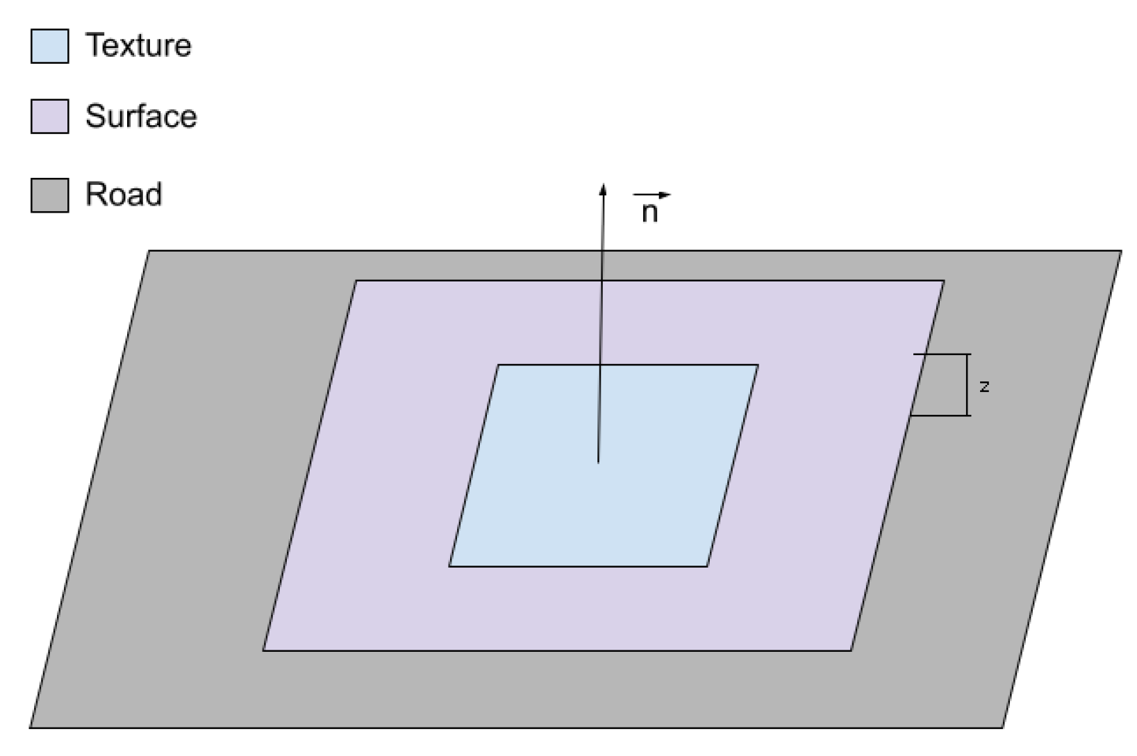
Finally, it is relevant to discuss the possible causes of error in the geolocation of signals that were correctly detected with the DL architecture. As can be seen in Figure 7, the checkboard used for calibration had to be placed on the right-hand side of the image to enable overlap with the lidar beams. This means that, although the reprojection errors were acceptable, they were smaller in the part of the image where the checkboard was placed. This implies that for signals appearing on the left side of the image (which will also be further from the MMS than a traffic sign on the right side of the image), it is possible that the reprojection will not be performed correctly and it will not be possible to geolocate the signal. This disadvantage could be solved in several ways. On the one hand, by redesigning the placement of the sensors so that the signs are captured more optimally: with the camera pointing to the right in the forward direction of the vehicle and positioned in such a way that the lidar system beams overlap with the central part of the image; on the other hand, by taking pictures more frequently, to avoid cases where there is no optimal position of a signal in any image. In any case, the results obtained with this system allow us to ensure that the methodology of calibration and fusion of 2D and 3D data are valid for the inventory of traffic signs.

5. Conclusions

This paper presents a method for the automatic recognition and geolocation of vertical traffic signs, so it can support those inventory works performed in road infrastructures. The input data are based on laser point clouds and images acquired with a low-cost mobile mapping system. In particular, the LiDAR employed is a Phoenix Scout Ultra 32, equipped with a Velodyne VLP-32C laser scanner. Data for this work was collected on a regional road in Avila (Spain). Furthermore, the method was validated using data recorded in the field as “ground truth” by an operator, finding that it can reliably detect, recognize and geolocate the vertical traffic signs. With the proposed method, it is possible to generate an automatic inventory of vertical traffic signs which can be visualized and managed in a WebGIS viewer based on Potree architecture. Therefore, this method can save resources in road maintenance works; to provide an inventory of all the vertical traffic signs with a manual operator requires a lot of time. With this approach an automatic inventory of vertical traffic signs can be obtained, and the data can be collected at conventional driving speeds, with no need for maintenance staff to measure outside of the vehicle (reducing risks and roadblocks). Future steps should be focused on refining the different methodological building blocks and broadening the type of infrastructure assets that can be geolocated with this methodology.

Author Contributions

Conceptualization, M.S. and D.G.-A.; methodology, M.S.; software, H.D., A.M. and M.S.; validation, M.S.; formal analysis, M.S. and D.G.-A.; investigation, H.D., A.M. and M.S.; resources, M.S. and D.G.-A.; data curation, H.D. and M.S.; writing—original draft preparation, H.D., A.M. and M.S.; writing—review and editing, M.S. and D.G.-A.; visualization, A.M.; supervision, M.S. and D.G.-A.; project administration, D.G.-A.; funding acquisition, D.G.-A. All authors have read and agreed to the published version of the manuscript.

Funding

The research leading to these results received funding from the Centro para el Desarrollo Tecnológico Industrial (CDTI) at the INROAD4.0 project (IDI-20181117) under the call 2018 for the strategic program CIEN. This work was partially supported by the Spanish Ministry of Science and Innovation through the grant FJC2018-035550-I funded by MCIN/AIE/10.13039/501100011033.

Informed Consent Statement

Not applicable.

Conflicts of Interest

The authors declare no conflict of interest.

References

  1. European Commission. State of Infrastructure Maintenance. Available online: https://ec.europa.eu/docsroom/documents/34561/attachments/1/translations/en/renditions/native (accessed on 3 August 2022).
  2. European Union Road Federation (ERF). ERF Road Statistics 2021. Available online: https://erf.be/statistics/ (accessed on 3 August 2022).
  3. Calvo-Poyo, F.; Navarro-Moreno, J.; de Oña, J. Road Investment and Traffic Safety: An International Study. Sustainability 2020, 12, 6332. [Google Scholar] [CrossRef]
  4. European Commission. Sustainable & Smart Mobility Strategy. Available online: https://transport.ec.europa.eu/transport-themes/mobility-strategy_en (accessed on 3 August 2022).
  5. European Court of Auditors. Towards a Successful Transport Sector in the EU: Challenges to be Addressed. Available online: https://www.eca.europa.eu/Lists/ECADocuments/LR_TRANSPORT/LR_TRANSPORT_EN.pdf (accessed on 3 August 2022).
  6. Alshehhi, R.; Marpu, P.R. Hierarchical graph-based segmentation for extracting road networks from high-resolution satellite images. ISPRS J. Photogramm. Remote Sens. 2017, 126, 245–260. [Google Scholar] [CrossRef]
  7. Huang, H.; Savkin, A.V.; Huang, C. Decentralized Autonomous Navigation of a UAV Network for Road Traffic Monitoring. IEEE Trans. Aerosp. Electron. Syst. 2021, 57, 2558–2564. [Google Scholar] [CrossRef]
  8. Balado, J.; González, E.; Arias, P.; Castro, D. Novel approach to automatic traffic sign inventory based on mobile mapping system data and deep learning. Remote Sens. 2020, 12, 442. [Google Scholar] [CrossRef] [Green Version]
  9. Holgado-Barco, A.; González-Aguilera, D.; Arias-Sanchez, P.; Martinez-Sanchez, J. Semiautomatic extraction of road horizontal alignment from a mobile LiDAR system. Comput.-Aided Civ. Infrastruct. Eng. 2015, 30, 217–228. [Google Scholar] [CrossRef]
  10. Holgado-Barco, A.; Gonzalez-Aguilera, D.; Arias-Sanchez, P.; Martinez-Sanchez, J. An automated approach to vertical road characterisation using mobile LiDAR systems: Longitudinal profiles and cross-sections. ISPRS J. Photogramm. Remote Sens. 2014, 96, 28–37. [Google Scholar] [CrossRef]
  11. Williams, K.; Olsen, M.J.; Roe, G.V.; Glennie, C. Synthesis of transportation applications of mobile LIDAR. Remote Sens. 2013, 5, 4652–4692. [Google Scholar] [CrossRef] [Green Version]
  12. Ma, L.; Li, Y.; Li, J.; Wang, C.; Wang, R.; Chapman, M.A. Mobile laser scanned point-clouds for road object detection and extraction: A review. Remote Sens. 2018, 10, 1531. [Google Scholar] [CrossRef] [Green Version]
  13. Soilán, M.; Sánchez-Rodríguez, A.; del Río-Barral, P.; Perez-Collazo, C.; Arias, P.; Riveiro, B. Review of Laser Scanning Technologies and Their Applications for Road and Railway Infrastructure Monitoring. Infrastructures 2019, 4, 58. [Google Scholar] [CrossRef] [Green Version]
  14. Plainis, S.; Murray, I.J.; Pallikaris, I.G. Road traffic casualties: Understanding the night-time death toll. Inj. Prev. 2006, 12, 125–138. [Google Scholar] [CrossRef]
  15. Chang, K.; Ramirez, M.V.; Dyre, B.; Mohamed, M.; Abdel-Rahim, A. Effects of longitudinal pavement edgeline condition on driver lane deviation. Accid. Anal. Prev. 2019, 128, 87–93. [Google Scholar] [CrossRef]
  16. Babić, D.; Babić, D.; Cajner, H.; Sruk, A. Mario Fioli Effect of Road Markings and Traffic Signs Presence on Young Driver Stress Level, Eye Movement and Behaviour in Night-Time Conditions: A Driving Simulator Study. Safety 2020, 6, 24. [Google Scholar] [CrossRef]
  17. Chen, T.; Lu, S. Accurate and Efficient Traffic Sign Detection Using Discriminative AdaBoost and Support Vector Regression; Accurate and Efficient Traffic Sign Detection Using Discriminative AdaBoost and Support Vector Regression. IEEE Trans. Veh. Technol. 2016, 65, 4006–4015. [Google Scholar] [CrossRef]
  18. Wang, G.; Ren, G.; Wu, Z.; Zhao, Y.; Jiang, L. A robust, coarse-to-fine traffic sign detection method. In Proceedings of the 2013 International Joint Conference on Neural Networks (IJCNN), Dallas, TX, USA, 4–9 August 2013; pp. 1–5. [Google Scholar] [CrossRef]
  19. Stallkamp, J.; Schlipsing, M.; Salmen, J.; Igel, C. The German Traffic Sign Recognition Benchmark: A multi-class classification competition. In Proceedings of the International Joint Conference on Neural Networks, San Jose, CA, USA, 31 July–5 August 2011; pp. 1453–1460. [Google Scholar] [CrossRef]
  20. Zhang, J.; Xie, Z.; Sun, J.; Zou, X.; Wang, J. A Cascaded R-CNN with Multiscale Attention and Imbalanced Samples for Traffic Sign Detection. IEEE Access 2020, 8, 29742–29754. [Google Scholar] [CrossRef]
  21. Cao, J.; Zhang, J.; Jin, X. A Traffic-Sign Detection Algorithm Based on Improved Sparse R-cnn. IEEE Access 2021, 9, 122774–122788. [Google Scholar] [CrossRef]
  22. Redmon, J.; Farhadi, A. YOLOv3: An Incremental Improvement. arXiv 2018. [Google Scholar] [CrossRef]
  23. Rajendran, S.P.; Shine, L.; Pradeep, R.; Vijayaraghavan, S. Real-Time Traffic Sign Recognition using YOLOv3 based Detector. In Proceedings of the 2019 10th International Conference on Computing, Communication and Networking Technologies, ICCCNT 2019, Kanpur, India, 6–8 July 2019. [Google Scholar] [CrossRef]
  24. Wan, J.; Ding, W.; Zhu, H.; Xia, M.; Huang, Z.; Tian, L.; Zhu, Y.; Wang, H. An Efficient Small Traffic Sign Detection Method Based on YOLOv3. J. Signal Process. Syst. 2021, 93, 899–911. [Google Scholar] [CrossRef]
  25. Arcos-García, Á.; Álvarez-García, J.A.; Soria-Morillo, L.M. Deep neural network for traffic sign recognition systems: An analysis of spatial transformers and stochastic optimisation methods. Neural Netw. 2018, 99, 158–165. [Google Scholar] [CrossRef] [Green Version]
  26. Jaderberg, M.; Simonyan, K.; Zisserman, A.; Kavukcuoglu, K. Spatial Transformer Networks. arXiv 2015. [Google Scholar] [CrossRef]
  27. Jin, J.; Fu, K.; Zhang, C. Traffic Sign Recognition With Hinge Loss Trained Convolutional Neural Networks. IEEE Trans. Intell. Transp. Syst. 2014, 15, 1991–2000. [Google Scholar] [CrossRef]
  28. Pu, S.; Rutzinger, M.; Vosselman, G.; Oude Elberink, S. Recognizing basic structures from mobile laser scanning data for road inventory studies. ISPRS J. Photogramm. Remote Sens. 2011, 66, S28–S39. [Google Scholar] [CrossRef]
  29. Riveiro, B.; Diaz-Vilariño, L.; Conde, B.; Soilán, M.; Arias, P. Automatic Segmentation and Shape-Based Classification of Retro-Reflective Traffic Signs from Mobile LiDAR Data. IEEE J. Sel. Top. Appl. Earth Obs. Remote Sens. 2016, 9, 295–303. [Google Scholar] [CrossRef]
  30. Yu, Y.; Li, J.; Wen, C.; Guan, H.; Luo, H.; Wang, C. Bag-of-visual-phrases and hierarchical deep models for traffic sign detection and recognition in mobile laser scanning data. ISPRS J. Photogramm. Remote Sens. 2016, 113, 106–123. [Google Scholar] [CrossRef]
  31. Arcos-García, A.; Soilán, M.; Alvarez-García, J.A.; Riveiro, B. Exploiting synergies of mobile mapping sensors and deep learning for traffic sign recognition systems. Expert Syst. Appl. 2017, 89, 286–295. [Google Scholar] [CrossRef]
  32. Schuetz, M. Potree: Rendering Large Point Clouds in Web Browsers Diplom-Ingenieur in Visual Computing. Diploma Thesis, Vienna University of Technology, Vienna, Austria, 2016. [Google Scholar]
  33. Velodyne LiDAR Inc. Velodyne LiDAR VLP-32C—Specifications Sheet. Available online: https://www.mapix.com/wp-content/uploads/2018/07/63-9378_Rev-D_ULTRA-Puck_VLP-32C_Datasheet_Web.pdf (accessed on 18 April 2022).
  34. He, K.; Zhang, X.; Ren, S.; Sun, J. Deep Residual Learning for Image Recognition. arXiv 2015. [Google Scholar] [CrossRef]
  35. Heikkila, J.; Silven, O. Four-step camera calibration procedure with implicit image correction. In Proceedings of the IEEE Computer Society Conference on Computer Vision and Pattern Recognition, San Juan, PR, USA, 17–19 June 1997; pp. 1106–1112. [Google Scholar] [CrossRef] [Green Version]
  36. Zhang, Z. A flexible new technique for camera calibration. IEEE Trans. Pattern Anal. Mach. Intell. 2000, 22, 1330–1334. [Google Scholar] [CrossRef]
  37. Zhou, L.; Li, Z.; Kaess, M. Automatic Extrinsic Calibration of a Camera and a 3D LiDAR Using Line and Plane Correspondences. In Proceedings of the 2018 IEEE/RSJ International Conference on Intelligent Robots and Systems (IROS), Madrid, Spain, 1–5 October 2018; pp. 5562–5569. [Google Scholar] [CrossRef]
  38. Martinez-Rubi, O.; Verhoeven, S.; Meersbergen, M. Van; Schuetz, M.; van Oosterom, P.; Gonclves, R.; Tijssen, T. Taming the beast: Free and open-source massive point cloud web visualization. Capturing Real. Forum 2015, 2015, 23–25. [Google Scholar] [CrossRef]
Figure 1. Case study. (a) low-cost mobile mapping system, with a Velodyne VLP-32C laser scanner and a manually mounted Sony A600 camera. (b) 6 km stretch of a regional road in the province of Ávila (Spain).
Infrastructures 07 00133 g001
Figure 2. High-level workflow of the method developed for traffic sign inventory.
Infrastructures 07 00133 g002
Figure 3. Workflow of the DL block, from an input image traffic signs are detected and hierarchically classified.
Infrastructures 07 00133 g003
Figure 4. Schematic representation of the YOLOV3 architecture.
Infrastructures 07 00133 g004
Figure 5. Classes and subclasses of the traffic signs selected.
Infrastructures 07 00133 g005
Figure 6. Camera-LiDAR calibration: Coordinate systems for spatial synchronization.
Infrastructures 07 00133 g006
Figure 7. Calibration between the LiDAR sensor and the camera. (a) image acquired of the checkboard. (b) point cloud acquired of the checkboard.
Infrastructures 07 00133 g007
Figure 8. Geolocation workflow for a single image with a traffic sign detected within the Deep Learning block.
Infrastructures 07 00133 g008
Figure 9. Camera-LiDAR calibration. (a) backward projection of point clouds on the image. (b) forward projection of the image pixel on the point cloud.
Infrastructures 07 00133 g009
Figure 10. Texture placement schema for the visualization of traffic signs with Potree.
Infrastructures 07 00133 g010
Figure 11. Example of an extreme situation where (a) Traffic sign is omitted by the manual labeller. (b) Traffic sign is detected by the deep learning architecture.
Infrastructures 07 00133 g011
Figure 12. 3D visualization of the classified traffic signs using Potree.
Infrastructures 07 00133 g012
Table 1. Training parameters.
ParametersYOLOv3Resnet152
OptimizerAdamSGD
Loss FunctionBinary Cross-EntropyCross-Entropy
Learning Rate0.0010.0001
Momentum0.90.9
Weight Decay0.00050.1
Batch Size168
Training Epochs100100
Table 2. Results of traffic signs detection using the deep learning architecture.
PrecisionRecallF-ScoreMean IoU
0.6110.8680.7170.685
Table 3. Confusion matrix of the traffic sign recognition results.
ProhibitionGive wayDangerMandatoryStopNo Entry
Prohibition4700001
Give way0150000
Danger0032000
Mandatory000100
Stop200000
No entry000001
Table 4. Prohibition subclasses analysis.
Number of Recognized Prohibition SignsNumber of Correct Predictions
3428
Table 5. Camera internal calibration: Results of the intrinsic parameters.
ParameterValue
Focal length (px)(4057.3, 4067.3)
Principal point [cx, cy] (px)(2978.03, 2001.68)
Image Size [rows, cols] (px)(4000, 6000)
Radial Distortion Coeffs.(−0.0749, 0.0976)
Intrinsic matrix (   4057.3 0 0 0 4067.3 0 2978.03 2001.68 1 )
Table 6. Error in the LiDAR-camera calibration process.
ParameterError
Translation0.0259 m
Rotation3.62°
Reprojection30.53 px
Table 7. Validation for the detection, recognition, and geolocation of traffic signs.
DetectedRecognized (Class)Recognized (Subclass)Geolocated
Number of signs45442234
% of signs95.74%97.77%88%75.5%
Table 8. Point cloud visualization with Potree: Generation and loading times.
Number of PointsGeneration Time (s)Loading Time (s)
43,387,673252
Publisher’s Note: MDPI stays neutral with regard to jurisdictional claims in published maps and institutional affiliations.

