Resilience of Railway Transport to Four Types of Natural Hazards: An Analysis of Daily Train Volumes

Abstract

A crucial step in measuring the resilience of railway infrastructure is to quantify the extent of its vulnerability to natural hazards. In this paper, we analyze the vulnerability of the German railway network to four types of natural hazards that regularly cause disruptions in German rail operations: floods, mass movements, slope fires, and tree falls. Using daily train traffic data matched with various data on disruptive events, we quantify the extent to which these four types of natural hazard reduce daily train traffic volumes. With a negative binomial count data regression, we find evidence that the track segments of the German railway network are most vulnerable to floods, followed by mass movements and tree-fall events. On average, floods reduce traffic on track segments by 19% of the average daily train traffic, mass movements by 16%, and tree fall by 4%. Moreover, when more than one type of natural hazard affects the track segment on the same day, train traffic on that segment falls by 34% of the average train traffic. Slope fires have an ambiguous and nonrobust effect on train traffic due to the reverse causality due to its triggering factors. This is the first study that attempts to rank different natural hazards according to their impact on railway traffic. The results have implications for the selection of resilience strategy and can help prioritize policy measures.

1. Introduction

A functioning and efficient transportation system is a basic requirement for a modern economy, supplying society with goods and services. Disruptions or breakdowns in the transportation system affect many areas of life, with prolonged disruptions having lasting impacts on administration and society. Natural hazards such as earthquakes or storms may have fatal impacts on the safe operation of both the rail infrastructure and may even threaten passengers’ lives [1,2]. The impact of disruptions caused by natural hazards can grow to enormous proportions, as recently demonstrated by the flood disaster in Germany and central Europe in July 2021. The heavy rainfall due to the low-pressure system Bernd caused severe flooding across the region that led to many fatalities and considerable damage to infrastructure [3]. For instance, around 600 km of the German railway lines were affected, some of which were completely destroyed. The reconstruction of these lines is predicted to take several years and estimated to cost around EUR 1.3 billion [4].

Compared to road transport, railway transport is especially vulnerable to traffic interruptions because of its relatively lower network density and hence fewer route alternatives [5]. In the event of a disruption, the track is immediately affected in its entirety due to its track-bound nature. Causes of railway disruptions are manifold, e.g., accidents, construction work, or damage to infrastructure, but among the most important of these causes is natural hazards [6,7]. As adverse weather and climate conditions trigger many if not most natural hazards [8], the increase in climate extremes is changing the frequency and magnitude of natural hazards, thereby increasing the vulnerability of the transportation sector [9,10]. According to Molarius et al. [11], the weather phenomena with the most potential harm to rail transport in temperate Central Europe are wind gusts, heat waves with temperatures above +25 °C, and heavy precipitation (>30 L/m² per day). In Germany, regional climate models predict a further increase in extreme climate events, particularly more intense heat waves and longer drought periods, as well as heavy precipitation and storms [12]. It is therefore likely in the future that disruptions to rail operations due to natural hazards will not only occur more frequently, but will also last longer and reach supraregional dimensions more often [13].

In the context of climate change, it is therefore of great importance to ensure rail operations are more resilient to natural hazards. The United Nations Office for Disaster Risk Reduction (UNISDR) defines resilience as:

The ability of a system, community or society exposed to hazards to resist, absorb, accommodate and recover from the effects of a hazard in a timely and efficient manner, including through the preservation and restoration of its essential basic structures and functions [14].

In terms of the transport sector, the European Committee for Standardization (CEN) defines resilience as the “ability to continue to provide service if a disruptive event occurs”. Service here means the safe and sustainable mobility of persons and goods from one point to another within a specified time [15]. The resilience of transport infrastructure is therefore the ability to withstand disruptive events and maintain capacity to provide mobility as a service. According to CEN [15], the resilience of an infrastructure to natural hazards comprises two aspects: absorption and recovery. Absorption is the ability to manage the adverse effects of the natural hazard upon impact, whereas recovery is the process of returning to the original level of service. The first aspect, absorption, by definition encompasses the vulnerability of the infrastructure, i.e., the propensity of the infrastructure to be adversely affected by natural hazards. The first step in measuring resilience is therefore to quantify the extent of an infrastructure’s vulnerability to natural hazards. In this study, we analyzed the vulnerability of railway infrastructure by taking daily train traffic volumes as the level of mobility service and investigating the extent to which the infrastructure is adversely affected by natural hazards using deviations from the standard level of service.

Only a handful of studies have evaluated the effects of natural hazards on railway traffic. Chan and Schofer analyzed the impact of hurricanes and snowstorms on service days lost on urban rail systems in the United States [16]. Kellermann et al. developed a flood damage model for estimating both the structural damage and economic losses to the railway infrastructure [7]. Janić used a deterministic approach to measure the resilience of the Shinkansen high-speed rail network to the Great East Japan Earthquake of 2011 [17]. All three studies have one thing in common: they attempted to measure resilience for isolated cases, either for specific catastrophic events [17] or for a specific type of natural hazard such as floods [7,18] or weather disruptions [16]. One study that investigated different types of disruptions on train delays is Xu et al. [19], but they focused mostly on technical train or infrastructure failures and lumped all natural hazards together into one category. To the best of our knowledge, no previous study has compared the effects of different types of natural hazards in a single empirical framework.

The objective of this study is to quantify the vulnerability of the German railway network to different types of natural hazards, thereby addressing the absorption aspect of infrastructure resilience. We focus on four types of natural hazards that regularly cause disruptions in German rail operations: floods, mass movements, slope fires, and tree falls. We match daily train traffic data with geospatial information on disruptive events along the railway network and conduct a negative binomial regression analysis to quantify the extent to which these natural hazards reduce daily train traffic volumes. Our study aims to answer the following research questions: (1) How do the different natural hazards affect daily train traffic volumes? (2) Which natural hazard has the strongest impact on daily train traffic volumes?

2. Materials and Methods

The empirical basis of this study revolves around two types of data: (1) daily train traffic data and (2) event data on the four different types of natural hazards. In the following sections, we describe each dataset in detail, explain how the datasets are matched, and elaborate on the regression models developed for the analyses.

2.1. Train Traffic Data

Quantifying vulnerability requires a measure of the level of mobility service a transport infrastructure provides. To represent the level of service provided by each track segment of the German railway network, we used data on daily train traffic from DB Netz AG, Frankfurt, a wholly owned subsidiary of Deutsche Bahn (DB) and the largest railway network operator in Germany. A track segment is defined as a section of the railway network between two operating points (Betriebsstelle) along a specific route (Strecke). For this study, DB Netz AG provided extensive panel data on train movement from 12 March 2018 to 31 December 2020 across all track segments of the railway network. For each track segment, the data contain information on whether it is single- or double-tracked as well as daily numbers of passing trains in both directions, counting freight trains as well as long- and short-distance passenger trains. The data consist of 10,705 track segments, of which 9988 have average traffic of at least one train per day within a given year.

The full unbalanced panel dataset consists of 10,040,607 observations. Each observation represents one track segment per day. Every track segment in the dataset therefore appears at most 1026 times, because there are 1026 days between 12 March 2018 and 31 December 2020. Similarly, each day appears at most 9988 times, because there are 9988 relevant track segments in the panel.

Table 1. Descriptive statistics of the variables in the train traffic data with N = 10,040,607 observations.

Variable	Mean	SD	Min	Max
Trains per day	93.84	91.19	0	1001
Single track	0.46	0.5	0	1

presents the descriptive statistics of the variables in the train traffic data. On average, close to 94 trains pass each track segment per day. The track segments are nearly equally distributed between single (46%) and double-tracked (54%).

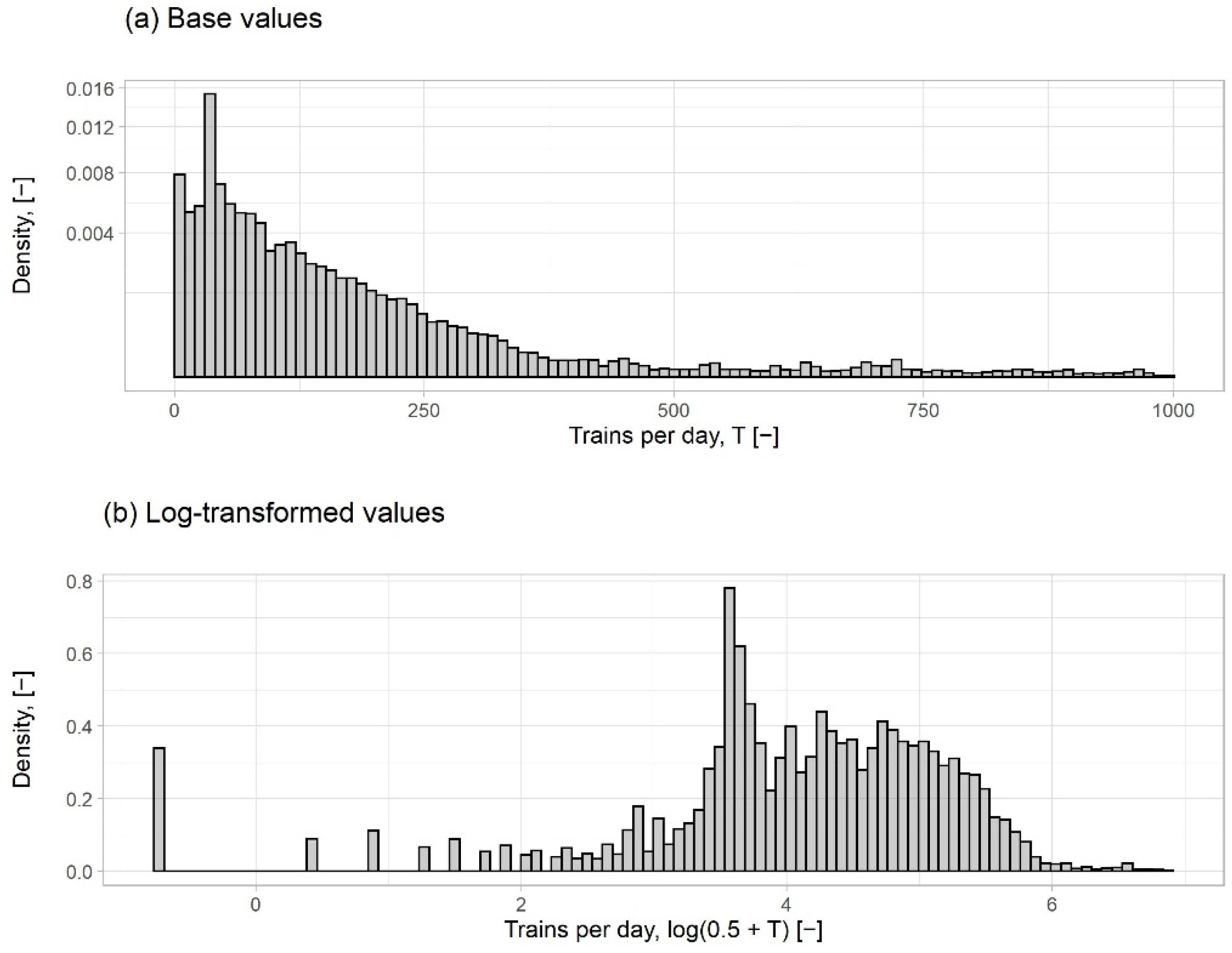
A histogram of daily train counts per day over the investigation period is presented in Figure 1. As expected of count data, the distribution is not normally distributed, as can be seen in Figure 1a, being truncated on the left with a mass of data points around zero. A standard method of dealing with truncated and highly right-skewed distributions is to take the logarithm. When zero values were present, as is common with count data, we used the continuity-corrected transformation $\log \left(0.5+x\right)$ for graphical purposes. After log-transforming (Figure 1b), the shape of the distribution was closer to the normal distribution. However, a mass of data points remained to the left of the distribution, representing the zero values in the untransformed count variable. These zero values were dealt with using the hurdle and zero-inflated models explained in Section 2.4.

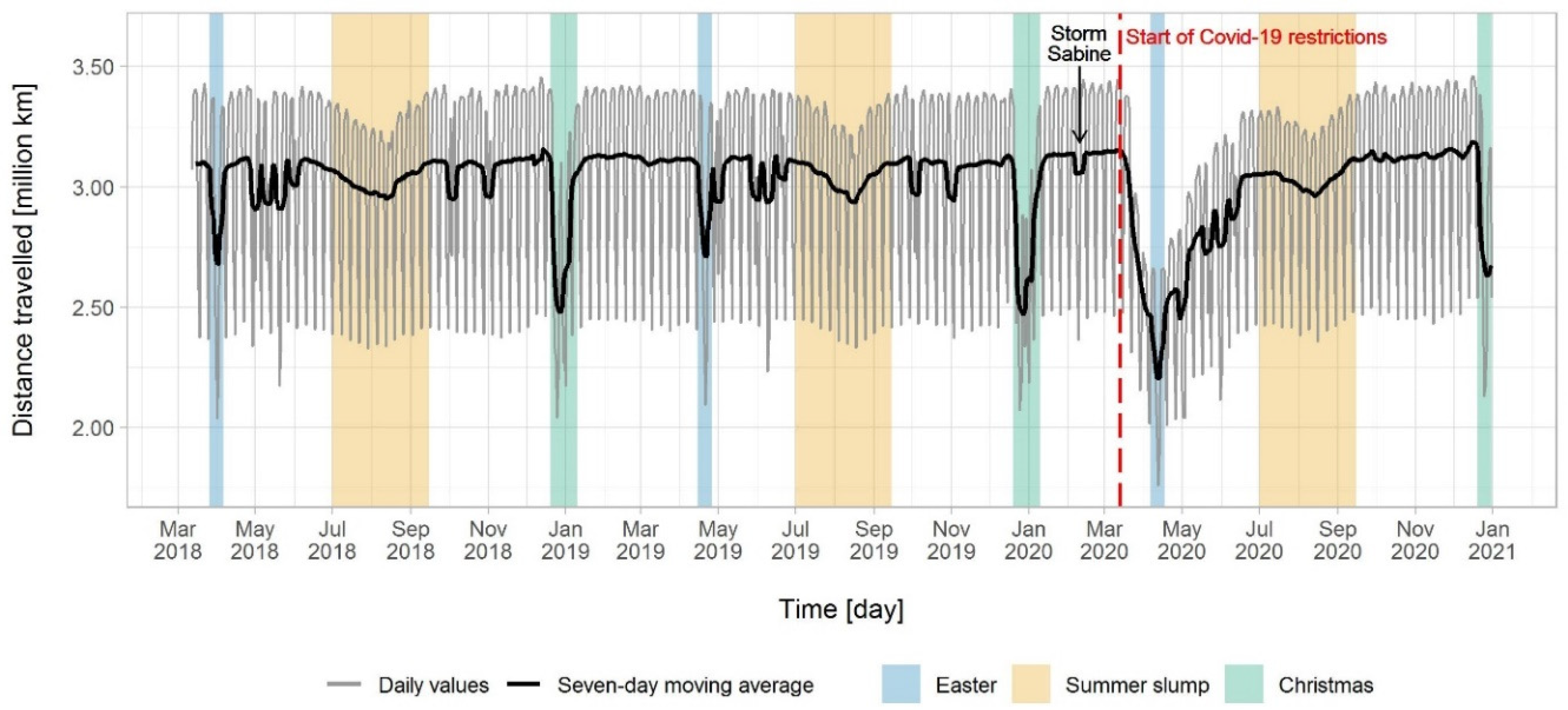
Figure 2 plots the time series of total distance travelled across the whole DB railway network over the sample period. The time series is relatively stable and varies between 2.0 to 3.5 million km travelled per day, with regular fluctuations between the weekdays and the weekends. Of note is the clear decrease in distance travelled during the beginning of the COVID-19 pandemic in March 2020, which took until October of the same year to return to pre-pandemic levels. Furthermore, seasonal variations occur during the German Easter and Christmas holidays. There is also a gradual drop in travelled distance around July that recovers by mid-September. This is when summer break takes place in schools and many employees take weeklong vacations, which the Germans call the summer slump or Sommerloch. Interestingly, despite the significant disruption in 2020 caused by the COVID-19 restrictions, the seasonal variations due to Easter and summer holidays are still clearly observable.

Figure 1. Histogram of daily train counts per day for a track segment with: (a) base values of trains per day and (b) log-transformed values of trains per day.

Figure 1. Histogram of daily train counts per day for a track segment with: (a) base values of trains per day and (b) log-transformed values of trains per day.

Figure 2. Total distance travelled throughout the Deutsche Bahn (DB) railway network over time.

Figure 2. Total distance travelled throughout the Deutsche Bahn (DB) railway network over time.

2.2. Event Data

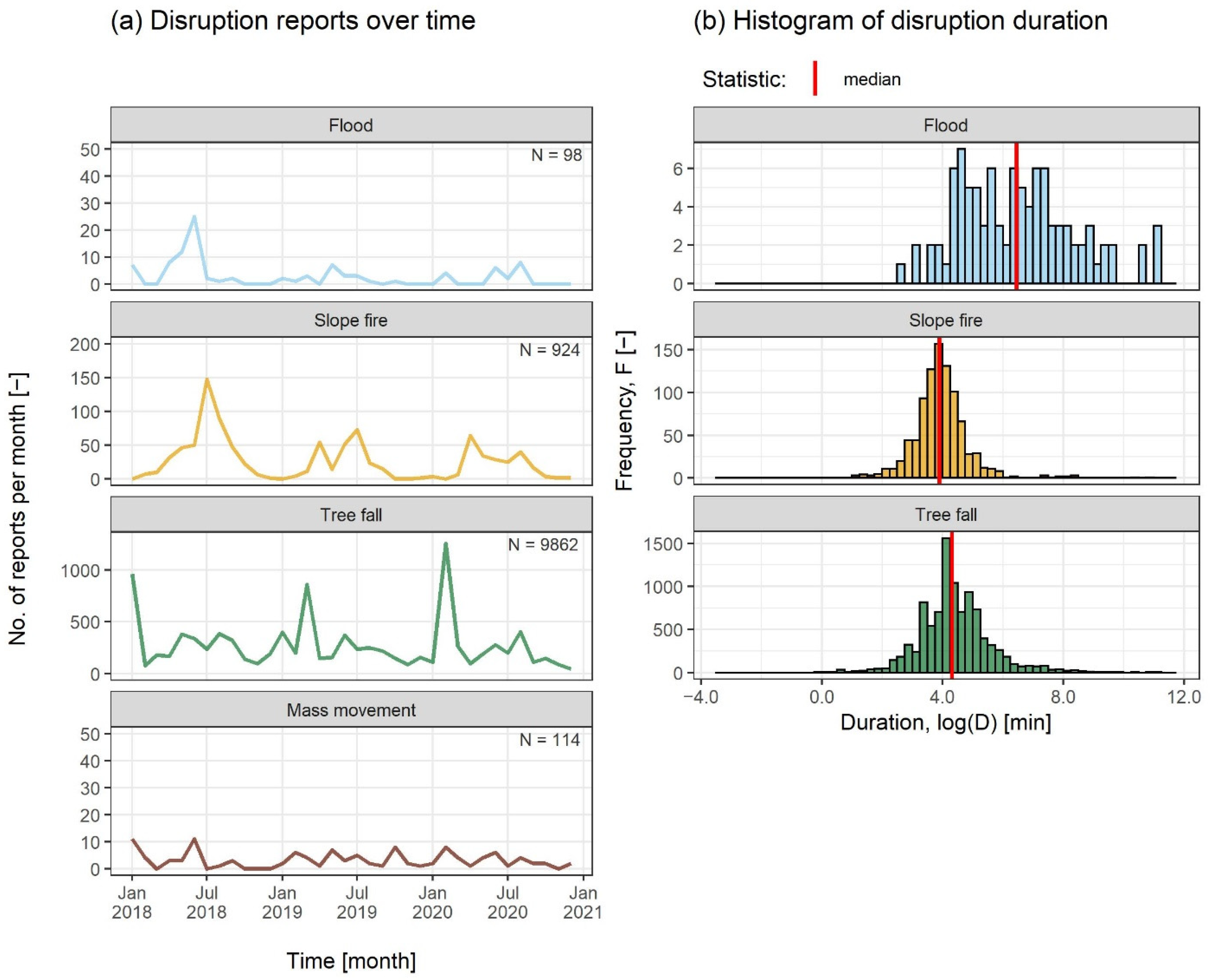
DB Netz AG provided event data from their accident database for four different types of natural hazards for the years 2018 to 2020: floods, mass movements, slope fires, and tree falls. We chose these processes because they regularly cause disruptions to German rail operations [13]. They differ in spatial extent, seasonal occurrence, and triggering factors, thereby covering a broad spectrum of natural event-related disturbances. Information about the date and geographical location of the events are provided in the database. The different natural hazards occur and are reported at different frequencies (

Table 2. Number of reports of the different natural hazards and the duration of the disruption.

Natural Hazard	No. of Reports	Mean Duration (in min) (± SD)	No. of Disruptions > 1 Day (% of Total No. of Reports)
Flood	98	4565.9 (±13,051.9)	32 (32.7%)
Mass movement	114
Slope fire	924	186.6 (±1981.4)	13 (1.4%)
Tree fall	9862	271.5 (±2219.5)	236 (2.4%)

Note: For mass movements, no information on disruption duration was provided.

), with tree falls having the most reports (9862), followed by slope fires (924 reports). Floods (98 reports) and mass movements (114 reports) have the least number of reports during the investigation period, suggesting that they seldom occur along the German railway network. The monthly distribution () shows that tree falls occur mainly during January to March, whereas slope fires occur predominantly from April to August (Figure 3a). Of note is the summer of 2018, where huge spikes in floods, gravitational mass movements, and slope fires can be observed. The summer of 2018 was one of the hottest and driest summers reported in Germany, leading to visible heat- and drought-induced disturbances in installations of the roadway and the control and safety technology [13]. Heavy thunderstorms with torrential rain and localized squalls in late summer caused disruptions due to tree falls, track undermining, and lightning strikes [13].

In all event datasets except for mass movements, information on the start and end times of every disruptive event is provided. The start time is when the event is first noticed, and the end time marks the time when the damage from the event is removed and operations can resume as scheduled. This information allowed us to calculate disruption duration in minutes for floods, slope fires, and tree fall events, shown in the second column of Table 2. The mean duration for all three types of natural hazards exceeds three hours, with floods averaging more than three days. The histograms of log-transformed disruption duration by natural hazard is presented in Figure 3b. The duration of flood events is more variable compared to tree falls and slope fires owing to the fewer number of reports. Nevertheless, it is clear that the curve for floods lies slightly to the right of the curves for slope fires and tree falls, and the median duration of flood events is longer. For floods, around one-third of all reported events last longer than one day, while the proportions of the events lasting longer than one day are very small for slope fires and tree falls (Table 2).

2.3. Matching Traffic and Event Data

Information on the geographic location of the disruptive events differs across event datasets. For the data on mass movements and tree falls, the route number and track kilometer associated with the location of the disruptive event are provided, allowing for a straightforward spatial matching with the train traffic panel. However, the datasets on slope fires and floods have no information on the route number or on the track kilometer where the event took place. Instead, the DB accident database assigns these events only to the nearest operating point. Note that an operating point could belong to intersecting routes on the network, and for every route to which it belongs, it has a different track kilometer. Slope fire and flooding events were therefore matched with the train traffic panel as follows: All track segments along different routes with endpoints associated with the corresponding operating point in the event dataset were counted as having the appropriate disruptive event. This means that each flood or slope fire event may be assigned to at least two track segments. The consequence of this relatively less accurate matching procedure is increased variability in the traffic values associated with slope fires and floods. As a result, slope fires and floods will have larger standard errors in the econometric analyses. This affects the hypothesis testing, potentially resulting in less statistically significant regression estimates.

Among the disruptive event reports present in the four events datasets, we successfully matched 98 reported flood disruptions (match rate 100%), 97 mass movements disruptions (85%), 904 slope-fire disruptions (98%) and 8724 tree-fall disruptions (88%) to a track segment in the train traffic dataset. Events that could not be matched with corresponding train data were those that occurred prior to 12 March 2018, or those that took place on track segments with mean traffic below one train per day. They were therefore excluded from the rest of the analyses.

2.4. Empirical Methods

Due to the count nature of the traffic variable in the dataset, conventional regression methods such as the ordinary least squares (OLS) would yield biased and inefficient results. Several count-data regression models have been proposed to deal with this problem: the Poisson regression model, the negative binomial regression model, the hurdle model, and the zero-inflated regression model.

The most common method for dealing with count data is the Poisson regression model, which yields efficient results as long as the conditional mean of the count variable is equal to its variance. This assumption, called equidispersion, is the biggest shortcoming of the Poisson regression model because most count data in the real word are over-dispersed [20]. In our dataset, the mean value of the train-count variable (93.3) is much smaller than the variance (8315.6), suggesting that the Poisson model might be inappropriate for our analysis. In such cases of overdispersion, the negative binomial regression model is a popular alternative to the Poisson because it introduces a dispersion parameter that allows the variance of the count variable to differ from the conditional mean [21,22], thereby loosening the equidispersion assumption.

One limitation of both the Poisson and negative binomial models, however, is the assumption that zeros and nonzeros come from the same data-generating process. For cases when this assumption is violated, both models insufficiently account for the heteroskedasticity caused by excess zeros. This is where the hurdle model [23] and the zero-inflated model [23,24] are useful. Both methods allow the data-generating processes for zeros and nonzeros to be different by modeling a second binary component that estimates the probability that the value of the dependent variable is zero.

The difference between the hurdle and the zero-inflated model lies in their assumptions about subpopulations of the data sample (in our case, subpopulations of track segments). The hurdle model assumes two types of track segments: (i) those where trains never pass and (ii) those where trains always pass at least once. The zero-inflated model instead assumes subpopulations of track segments where: (i) trains never pass or (iii) trains can pass, but not always [25,26]. More technically, the hurdle model separately estimates the zero values (generated by subpopulation (i)) from the count component of positive values (generated by (ii)). In contrast, the zero-inflated approach, although having a similar binary component estimating “structural” zeros from subpopulation (i), allows the count component to take both positive and zero values (i.e., “sampling” zeros).

In the case of train traffic, we can think of a subpopulation of tracks segments described in (i), i.e., where trains never pass, to be the track segments belonging to decommissioned routes. However, given that our dataset includes only track segments with at least one train per day on average, decommissioned routes and other track segments where trains never pass throughout the investigation period do not appear in the data. Therefore, in our dataset, the zeros and the nonzeros can be safely assumed to come from the same data-generating process, making a hurdle or a zero-inflated model superfluous. For this reason, we employed a negative binomial regression model to estimate the effect of natural hazards on train traffic in track segments.

2.4.1. Negative Binomial Regression Model

The negative binomial regression model estimated from the pooled panel dataset takes the form

$$\log \left(y_{it}\right)={\beta }_0+{\mathsf{\beta }}_1^{\prime }NatHa{z}_{it}+{\mathsf{\beta }}_2^{\prime }{z}_i+u_{it}$$

(1)

where the dependent variable $y_{it}$ is the count variable for the number of trains that pass through track segment $i$ on day $t$, and $NatHa{z}_{it}$ is a vector of mutually exclusive dummy variables indicating the occurrence of each type of natural hazard in track segment $i$ on day $t$. The dummy variables in $NatHa{z}_{it}$ are as follows: flood only, mass movement only, slope fire only, tree fall only, and two or more natural hazard events. This distinction allowed us to separately identify the individual effects of each natural hazard. The base variable is when no natural hazard event occurs.

The vector $z_{it}$ represents the control variables, namely whether a track segment is single-tracked, and dummy variables for day of the week, month, and year. The week dummies (with Friday as the base variable) control for weekday and weekend variation. The month dummies (with January as the base) control for seasonal effects. The year dummies (with 2018 as the base) control for the fact that variations in train traffic differed substantially during the COVID-19 pandemic (year 2020) compared to the other years in the sample. The parameter ${\beta }_0$ is a constant term that represents the log number of trains when all dummy variables are at their base levels. Finally, $u_{it}$ is an error term.

Assuming a negative binomial distribution for $y_{it}$ conditioned on all the regressors in (1), denoted $x_{it}=\left(NatHa{z}_{it},z_{it}\right)$, one parametrization of the probability density function of $y_{it}|x_{it}$ is

$$f\left(y_{it}|x_{it}\right)=\frac{\mathsf{\Gamma }\left(y+\theta \right)}{\mathsf{\Gamma }\left(\theta \right)·y!}·\frac{{\mu }^y{\theta }^{\theta }}{{\left(\mu +\theta \right)}^{y+\theta }}$$

(2)

where $\theta$ is the dispersion parameter and $\mathsf{\Gamma }\left(·\right)$ is the gamma function. This density function has conditional mean $\mu$ and conditional variance $=\mu +\frac{\mu }{\theta }$. Note that the value of $\theta$ determines whether the equidispersion assumption of the Poisson model holds, i.e., as $\theta$ approaches infinity, the conditional variance approaches the mean, and the distribution approximates a Poisson distribution. A maximum likelihood estimation is applied to the negative binomial model in (2) to obtain estimates of the parameter coefficients in (1).

The parameter of interest in Equation (1) is ${\mathsf{\beta }}_1$, which is the coefficient vector of the variables indicating the occurrence of a natural hazard event. Our hypothesis is the following: the occurrence of a natural hazard reduces the number of trains passing by a track segment. We therefore expect negative and significant values for the parameter coefficients ${\mathsf{\beta }}_1$.

2.4.2. Estimating the Effect Sizes of the Natural Hazard Events on Train Traffic

Although the signs and statistical significance of the coefficients could be easily obtained from the regression model in (1), the size of the effects in terms of reductions in the number of trains could not be obtained directly from ${\mathsf{\beta }}_1$ due to the logarithmic nature of the models. To obtain the size of each natural hazard’s effect on train traffic, we computed the average marginal effect (AME). The AME is calculated from the predicted values of the dependent variable $y_{it}$ in its base (non-logarithmic) form, i.e., the predicted number of trains per day. The marginal effect of a dummy variable (e.g., flood) is the difference in the predicted number of trains when the dummy variable has a value of one (i.e., when a flood occurs) versus the base variable (no disruptive event). Since the negative binomial regression is nonlinear, the predicted value and marginal effect depend on the values of all the regressors on the righthand side of Equation (1). This means that the marginal effects differ across all observations in the dataset. When the marginal effects are averaged over all observations, the result is the AME. In our study, the AMEs represent the average deviation in the number of trains per day compared to the base variable (no disruptive event). Using 95% confidence intervals, an estimate of the AME is statistically significant if confidence interval does not include zero. If the confidence interval includes zero, this means that the AME is not significant at the 5% level or that the train count during an event is not statistically different from the train count when no disruptions occur.

3. Results

3.1. Descriptive Statistics

The first column of

Table 3. Descriptive statistics and results from the regression analysis.

Categories	No. of Observations per Category	Median Trains per Day (Log-Transformed Values)	Average Marginal Effect (AME)
			Deviation in Number of Trains (±SD)	95% Confidence Interval
No disruptive event	10,028,672	4.2
Flood	802	4.0	−17.5 (± 2.0)	(−21.5, −13.5)
Mass movement	90	4.3	−14.8 (± 6.2)	(−27.0, −2.6)
Slope fire	3052	4.5	+2.6 (± 1.3)	(0.05, 5.2)
Tree fall	7975	4.0	−4.0 (± 0.7)	(−5.4, −2.7)
2+ disruptive events	16	3.7	−31.5 (± 11.7)	(−54.5, −8.6)
Total no. of observations	10,040,607

presents the frequency counts of the natural hazard events in the matched traffic and event datasets. Note that the counts of disruptive event differs from the number of reports in Table 2 for three reasons: First, one reported disruption could span several days, and each day is counted separately in the matched panel. Second, several reports could be filed for the same track segment on the same day, and third, for slope fires and floods, one report is matched to at least two track segments because only information on the nearest operating point is provided. Looking at the different categories, about 99.88% of the observations belong to the category “no disruptive event”, i.e., no natural hazard event occurred in that specific track segment on that specific day. In other words, disruptions due to either floods, mass movements, slope fires, or tree falls occur in only 0.12% of the observations. The smallest category with only 16 observations is the category of track segments hit by two or more types of natural hazard in the same day. Flood and tree fall events are the two natural hazards that most often occur on the same day as another event.

Figure 4 presents box plots of the train traffic distributions on days with and without natural hazard events. The exact values of the median in the box plots can be found in the second column of Table 3. Compared to days with no disruptive events, days with disruptions due to tree falls and floods have a noticeably lower median, which is statistically different from days without disruptive events based on the Wilcoxon two-sample test. This descriptive result supports our hypothesis. The difference is particularly striking on days with at least two natural hazard events, albeit not statistically significant due to the low number of observations in the sample. On days with mass movements, we found no discernable difference. Days with slope fires have a higher median, on average, than days with no disruptive events, an outcome that we discuss in detail in Section 4.

Although these results already provide an indication of how natural hazards affect train traffic, other factors that may influence this relationship, for instance, seasonal variation, are not taken into account. Controlling for these other factors involves regression analysis, the results of which we present in the next section.

3.2. Results from the Regression Analysis

Table 4. Regression estimates.

	Dependent Variable: Trains per Day
Variable	Negative Binomial (1)	Poisson (2)	Hurdle (3)	Zero-Inflated (4)
Tree fall only	−0.044 ***	−0.088 ***	−0.064 ***	−0.064 ***
	(0.008)	(0.007)	(0.007)	(0.007)
Slope fire only	0.027 *	0.018	0.016	0.016
	(0.014)	(0.012)	(0.012)	(0.012)
Flood only	−0.206 ***	−0.156 ***	−0.184 ***	−0.184 ***
	(0.026)	(0.022)	(0.024)	(0.024)
Gravitational mass movement only	−0.172 *	−0.219 ***	−0.194 **	−0.193 **
	(0.079)	(0.057)	(0.070)	(0.070)
Two or more disruptive events	−0.409 *	−0.606 **	−0.441 **	−0.443 **
	(0.188)	(0.187)	(0.167)	(0.167)
Single-tracked	−1.282 ***	−1.283 ***	−1.255 ***	−1.255 ***
	(0.0005)	(0.0004)	(0.0004)	(0.0004)
Constant	Yes	Yes	Yes	Yes
Week effects	Yes	Yes	Yes	Yes
Month effects	Yes	Yes	Yes	Yes
Year effects	Yes	Yes	Yes	Yes
Observations	10,040,607	10,040,607	10,040,607	10,040,607
Log likelihood	−52,983,781	−231,628,464	−52,332,085	−52,332,078
Dispersion parameter (θ)	1.837 *** (0.001)
Akaike Information Criterion (AIC)	105,967,614	463,256,979	104,664,276	104,664,261

Notes: * p < 0.05; ** p < 0.01; *** p < 0.001; standard errors in parentheses.

presents the estimation results of the negative binomial regression model in column (1). To check for robustness of the results, columns (2) to (4) present the estimates of the other count data models discussed in Section 2.4. The full regression table with the coefficient estimates and standard errors of all independent variables is provided in Appendix A 

Table A1. Full regression table.

	Trains per Day
Variable	Negative Binomial (1)	Poisson (2)	Hurdle (3)	Zero-Inflated (4)
Tree fall only	−0.044 ***	−0.088 ***	−0.064 ***	−0.064 ***
	(0.008)	(0.007)	(0.007)	(0.007)
Slope fire only	0.027 *	0.018	0.016	0.016
	(0.014)	(0.012)	(0.012)	(0.012)
Flood only	−0.206 ***	−0.156 ***	−0.184 ***	−0.184 ***
	(0.026)	(0.022)	(0.024)	(0.024)
Gravitational mass movement only	−0.172 *	−0.219 ***	−0.194 **	−0.193 **
	(0.079)	(0.057)	(0.070)	(0.070)
Two or more disruptive events	−0.409 *	−0.606 **	−0.441 **	−0.443 **
	(0.188)	(0.187)	(0.167)	(0.167)
Single-tracked	−1.282 ***	−1.283 ***	−1.255 ***	−1.255 ***
	(0.0005)	(0.0004)	(0.0004)	(0.0004)
Day of the week: Saturday	−0.210 ***	−0.208 ***	−0.198 ***	−0.198 ***
	(0.001)	(0.001)	(0.001)	(0.001)
Day of the week: Sunday	−0.316 ***	−0.320 ***	−0.295 ***	−0.295 ***
	(0.001)	(0.001)	(0.001)	(0.001)
Day of the week: Monday	−0.060 ***	−0.075 ***	−0.060 ***	−0.060 ***
	(0.001)	(0.001)	(0.001)	(0.001)
Day of the week: Tuesday	−0.0001	−0.0005	−0.001	−0.001
	(0.001)	(0.001)	(0.001)	(0.001)
Day of the week: Wednesday	0.007 ***	0.008 ***	0.006 ***	0.006 ***
	(0.001)	(0.001)	(0.001)	(0.001)
Day of the week: Thursday	0.001	0.003 ***	0.001	0.001
	(0.001)	(0.001)	(0.001)	(0.001)
Month: February	0.022 ***	0.027 ***	0.021 ***	0.021 ***
	(0.001)	(0.001)	(0.001)	(0.001)
Month: March	−0.007 ***	−0.003 ***	−0.006 ***	−0.006 ***
	(0.001)	(0.001)	(0.001)	(0.001)
Month: April	−0.082 ***	−0.079 ***	−0.076 ***	−0.076 ***
	(0.001)	(0.001)	(0.001)	(0.001)
Month: May	−0.041 ***	−0.041 ***	−0.037 ***	−0.037 ***
	(0.001)	(0.001)	(0.001)	(0.001)
Month: June	−0.007 ***	−0.005 ***	−0.003 **	−0.003 **
	(0.001)	(0.001)	(0.001)	(0.001)
Month: July	−0.005 ***	−0.003 *	0.004 **	0.004 **
	(0.001)	(0.001)	(0.001)	(0.001)
Month: August	−0.019 ***	−0.017 ***	−0.008 ***	−0.008 ***
	(0.001)	(0.001)	(0.001)	(0.001)
Month: September	0.010 ***	0.016 ***	0.017 ***	0.017 ***
	(0.001)	(0.001)	(0.001)	(0.001)
Month: October	0.002	0.008 ***	0.010 ***	0.010 ***
	(0.001)	(0.001)	(0.001)	(0.001)
Month: November	0.010 ***	0.015 ***	0.013 ***	0.013 ***
	(0.001)	(0.001)	(0.001)	(0.001)
Month: December	−0.026 ***	−0.028 ***	−0.023 ***	−0.023 ***
	(0.001)	(0.001)	(0.001)	(0.001)
Year: 2019	0.001	0.001	−0.001	−0.001
	(0.001)	(0.001)	(0.001)	(0.001)
Year: 2020	−0.023 ***	−0.022 ***	−0.025 ***	−0.026 ***
	(0.001)	(0.001)	(0.001)	(0.001)
Constant	5.043 ***	5.042 ***	5.048 ***	5.048 ***
	(0.001)	(0.001)	(0.001)	(0.001)
Observations	10,040,607	10,040,607	10,040,607	10,040,607
Log-likelihood	−52,983,781	−231,628,464	−52,332,085	−52,332,078
Dispersion parameter (θ)	1.837 *** (0.001)
Akaike information criterion (AIC)	105,967,614	463,256,979	104,664,276	104,664,261

Notes: * p < 0.05; ** p < 0.01; *** p < 0.001; standard error in parentheses.

.

The log-likelihood and the Akaike information criterion (AIC) provide an indication of the fit of the four count-data models. The higher the log-likelihood and the lower the AIC, the better the model fit. Comparing the log-likelihoods and AIC statistics of all four models, the Poisson model in column (2) of Table 4 is substantially inferior to the negative binomial, hurdle, and zero-inflated models, which indicates that overdispersion is a major issue in the data. The estimated dispersion parameter in the negative binomial model is much smaller (1.87) compared to the mean of the dependent variable (93.8), suggesting that the equidispersion assumption does not hold (recall that equidispersion holds if the dispersion parameter approaches infinity).

After overdispersion was corrected using the negative binomial regression, correcting for zero values no longer provided substantial improvement in the fit of the model. The hurdle and zero-inflated models in columns (3) and (4) of Table 4 have almost the same log-likelihoods and AIC values as the negative binomial in column (1). This is to be expected as our dataset already excludes track segments with fewer than one train per day on average.

Turning now to the parameter estimates, tree fall, flood, and mass movements have negative and significant coefficients in all count data models. This confirms our hypothesis that days with floods, mass movements, or tree-fall events have fewer passing trains compared to days with no disruptions, even after controlling for seasonal and confounding factors. Furthermore, the coefficients are negative and significant in all models, proving that these results are robust to model choice. For slope fires, the coefficients are positive but insignificant in all models except the negative binomial regression. This means that although we obtained a significant estimate, the result does not survive the use of other count-data models. Nevertheless, the positive coefficient in the negative binomial regression warrants deeper consideration, and can be explained by the triggering factors peculiar to slope fires, which we discuss extensively in Section 4.

While Table 4 provides information on the direction and significance of the different natural hazards, the nonlinearity of the regression models makes the magnitude of the coefficients difficult to interpret. For this reason, in Figure 5, we converted the effects into deviations in the number of trains per day via the AMEs and their 95% confidence intervals. The zero line intersecting a confidence interval means that there is no difference in the daily number of trains compared with days without disruptions. Exact values of the AMEs and their confidence intervals can be found in the last two columns of Table 3. Days with two or more natural hazard events have around 32 fewer trains than days without disruptions. This is one -third of the average number of trains per day across all observations (Table 1) and is by far the largest effect. In case of a flood event, there are, on average, 18 fewer trains, reducing the average number of trains by almost one-fifth. On days with mass movement events, the number of trains is lower by around 15, while days with tree-fall events have the smallest effect of only four fewer trains. For floods, mass movements, and tree falls, the AMEs are statistically significant. Looking at the slope-fire variable, the AME is positive at a value of two, meaning that days with slope fires have, on average, two trains more than days without disruptions. However, this estimate is barely significant, with a confidence interval that touches the y-axis at zero.

4. Discussion

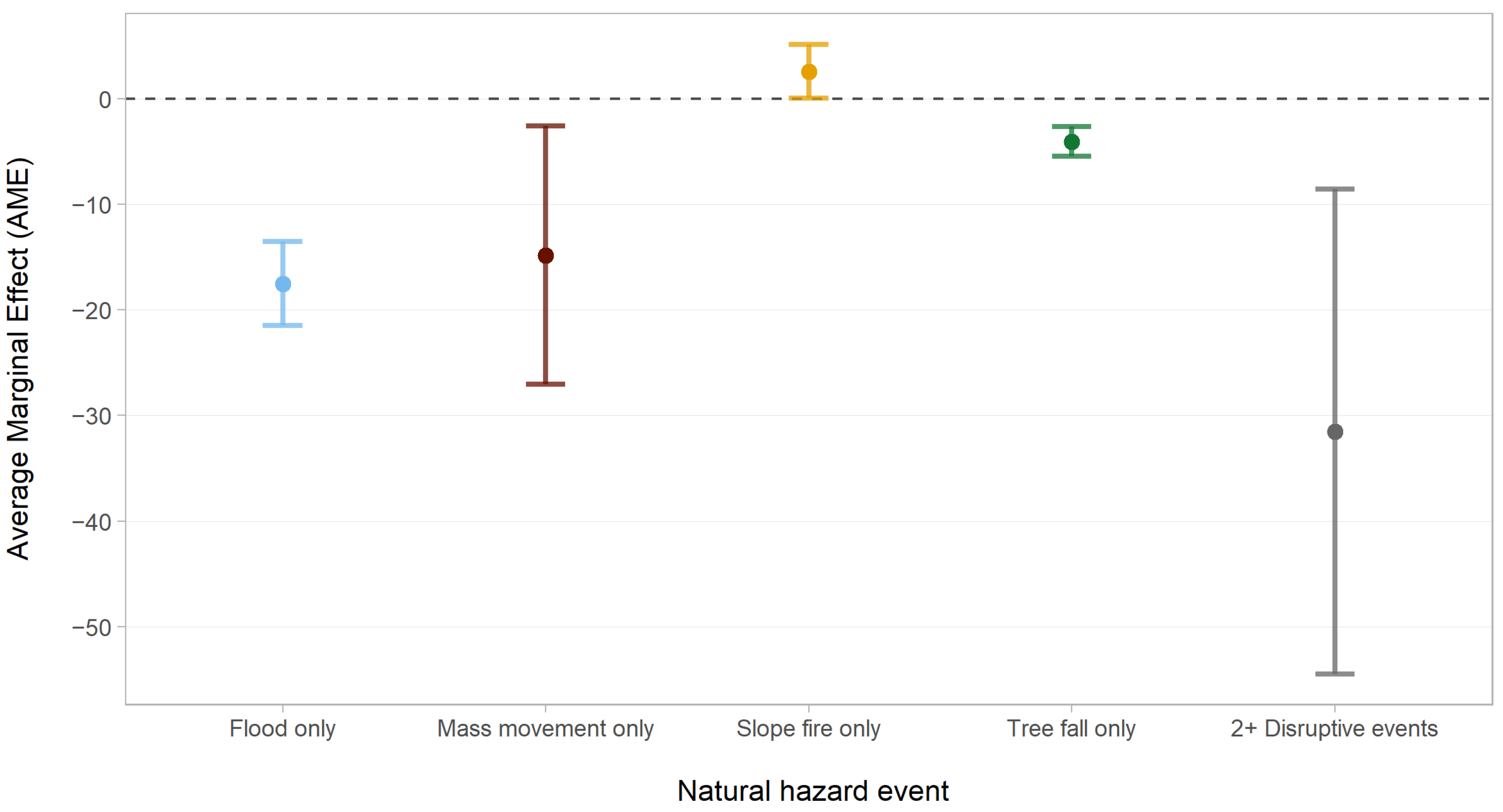
In this study, we analyzed the impact of four different types of natural hazard on railway traffic, which differ in their dimension, spatial distribution and extent, frequency of occurrence, and triggering factors. Mass movements are a major threat to infrastructure in alpine environments (e.g., [27]). In countries such as Germany, railway lines running along river valleys in middle mountain regions are particularly at risk (e.g., [28]), and the events are predominantly small with local effects: only a small number of events related to mass movements are recorded in the event database. When events occur infrequently, other more pressing matters may overshadow the salience of these events, thereby making infrastructure managers more prone to being underprepared when they happen. As a result, the impact of a single infrequent event can be substantial [11]. This could partially explain what we observed in our results, where the two most infrequent events in our dataset, floods and mass movements, have the largest effects on daily traffic among the natural hazards analyzed in this study (Figure 5). A recent example of a large mass movement event with a major impact on the European railway traffic is the Kestert rock fall in March 2021, which took place in the Upper Middle Rhine valley. This disaster resulted in the months-long closure of Europe’s busiest freight train route between Genoa and Rotterdam [29].

The seasonal distributions of flood, mass movement, and tree fall events are quite similar, suggesting that the triggering factors for these processes are closely related. Precipitation is a major trigger of floods and mass movements, specifically heavy precipitation events (>20 L/m² per day) or prolonged precipitation that lasts over several days. Tree-fall hazards are predominantly associated with storm events or strong wind gusts, which are often accompanied by heavy precipitation. Depending on the triggering factor, floods and tree-fall events can either be of local, e.g., thunderstorms in summer, or of regional/nationwide distribution, e.g., a winter storm caused by a large-scale low-pressure area. In the investigation period of 2018 to 2020, both types of triggering events occurred, e.g., the low-pressure area Nadine in August 2018 and Orkan Sabine in February 2020. The occurrence of storm and precipitation events are exogenous and are beyond the influence of infrastructure managers. Nevertheless, one preventive measure in the event of a storm warning is the partial or complete cessation of train operations. Shortly before Orkan Sabine hit Germany in February 2020, the DB put a nationwide stop on all its long-distance trains [30], resulting in a slump in travelled kilometers, which can be observed in Figure 2. Such measures might partially explain why storm-induced hazard events, particularly floods, mass movements, and tree falls, have a significant influence on the number of trains.

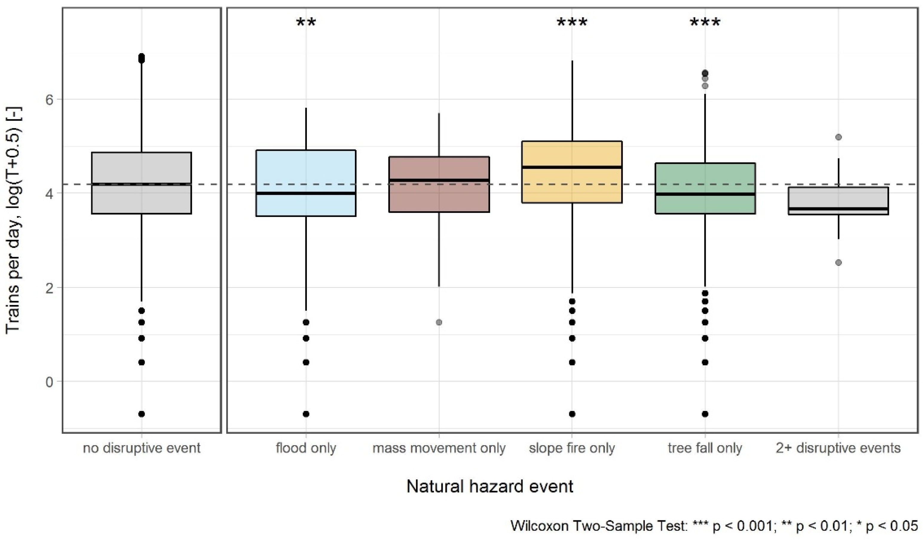
The results of the regression analysis showed that the number of trains fell during days with flood, mass movement, and tree-fall events, which supports our hypothesis. For slope fire events, however, we observed the opposite effect: the number of trains was higher than the average. This can be explained by the triggering factors that are peculiar only to slope fires. Dry vegetation and soils represent initial situations conducive to fires, but events are necessary for their initiation, e.g., sparks caused by technical defects on trains or discarding of burning cigarette butts. Therefore, while the occurrence of floods, mass movements, and tree falls is mainly caused by external factors and not by train operation itself, the occurrence of slope fires is related to the volume passing trains. Some studies have shown that slope fires are frequently caused by fixed brakes [31,32], making slope fires more likely to occur on lines with high train traffic volume, especially freight traffic. In other words, more trains passing a track segment could increase the probability that, under certain conditions, a train ignites a fire in a nearby embankment. If there is a positive feedback effect of the number of passing trains on the incidence of slope fires, the coefficients that are estimated by the regression model will be upward-biased [33]. This is because the relationship between slope fires and traffic consists of two opposing effects: (i) the positive effect from the fact that more passing trains could result in more slope fires, and (ii) the negative effect from the temporary track closures once a slope fire breaks out. These two effects cancel each other out, making the net effect ambiguous. In Table 4 and Figure 5, the estimates show that the net effect is positive, suggesting that the positive effect of (i) trumps the negative effect of (ii). This is not surprising as the temporary track closures due to slope fires are brief (Table 2). The ambiguity of the net effect is reflected in the coefficient of slope fires being significant in only one of the four regression models. Because of the estimation bias caused by (i), we cannot definitively conclude that the impact of slope fires on train traffic is different from zero. A deeper investigation is required that either calculates the size of the estimation bias or removes the estimation bias altogether via instrumental variables.

To answer the questions we posed at the beginning of this study, we estimated the effect sizes using average marginal effects (Figure 5). The results revealed that floods have the strongest impact on the railway system in terms of reduction in train traffic on the affected lines. Mass movements are ranked second, while tree fall events have the smallest impact. This implies that the German railway network is more vulnerable to and potentially less resilient against floods and mass movements than to tree falls. These results, i.e., the extent to which the infrastructure is vulnerable to a specific type of natural hazard, may have implications on the selection of the most appropriate resilience strategy.

According to Chan and Schofer, there are three resilience strategies that transportation systems can employ against natural hazards: hardening, redundancy, and elasticity [16]. For single tree-fall events that reduce daily train traffic by only a few trains, hardening measures may suffice. Hardening measures, such as protective walls, levees, and rock fall nets, are widespread and diverse on the German rail network. Hardening measures alone, however, may not be enough for larger natural hazard events. For events such as floods or mass movements with more substantial negative effects, additional redundancy and elasticity measures might be necessary. Unfortunately, redundancy measures are difficult to implement in railway systems due in part to the prevalence of single-line tracks, the lack of excess capacity, and the limited routing possibilities [5]. Nevertheless, identifying alternate lines as potential detour routes is a viable strategy that can increase resilience (e.g., [34]). The relative infeasibility of redundancy measures for railway makes elasticity measures the second-best alternative to minimize the damage caused by natural hazards. The temporary local or nationwide suspension of train services is a frequent practice in Germany, often implemented in the event of storm warnings or forecasted heavy snowfall.

The occurrence and hence the impact of all four types of natural hazards analyzed in this paper can be influenced by the trackside vegetation, both positively and negatively. Optimized vegetation management is therefore a crucial tool for a more resilient railway traffic. By choosing appropriate tree species and understory vegetation, the risks of tree falls and slope fires can be minimized (e.g., [35]). Additionally, appropriate vegetation has positive impacts on slope stability [36] and can reduce the erosive potential of slopes and railroad embankments during (heavy) precipitation events.

The frequency of simultaneous natural hazards affecting a track segment is very low; however, the importance of simultaneously occurring events and the associated damages and disruptions should not be underestimated. Despite the large confidence intervals of two or more disruptive events in Figure 5, we still identified a statistically significant effect that is at least twice as large as the effect of any natural hazard on its own. There are several reasons for the co-occurrence of different natural hazards in our study having such a low frequency. We assigned the events to track segments, which may be too detailed a spatial resolution, as a track segment is, on average, 6.9 km long. Further uncertainty arises from the event data, since the location is not always exact, so that spatially close events could theoretically have occurred at the same site. Since all the events occurred in the past and are predominantly small events that have no visible long-term traces in the landscape, the exact location can be retrospectively determined only in individual cases. For slope fires and floods, exact localization is not possible at all, since the events in the dataset are only assigned to the nearest operating point. Moreover, although reports were each assigned to one event category, an event can also represent a combination of different processes, e.g., the uprooting of trees due to mass movements or flash floods. Furthermore, the dataset has a short time span of only three years. If we were to study simultaneously occurring events, a route-level analysis with a longer time series of at least 10 years would be more appropriate. Despite these limitations, however, we are convinced that our study demonstrates the potential of matching natural hazard event data with train traffic data. Further efforts should be directed toward this previously under-represented area of rail transportation research.

5. Conclusions

In this study, we analyzed the impact of four different types of natural hazard in terms of the reduction in daily train volumes, and identified floods as having the strongest effect. We are the first to use a multihazard approach to attempt to rank different natural hazards according to their impact on railway traffic, the results of which can help to prioritize appropriate resilience strategies.

The results of this study open the door to further research, ideally with a dataset that has a wider spatial and temporal coverage. Not only will this capture more of the relatively infrequent events, such as simultaneously occurring natural hazards, but it will also provide enough information for forecasting trends in the effects of natural hazards. Furthermore, other potentially confounding factors must be taken into consideration, such as weather and other causes of railway disruptions, which is necessary in order to remove reverse causality and other potential endogeneity in train traffic. With this, less ambiguous and more robust measures of the vulnerability of railway infrastructure can be estimated, especially for natural hazards such as slope fires.

We concentrated on four natural hazards, but the same empirical methodology can be applied to any other type of natural hazard, depending on which threats to the railway network are being considered. Furthermore, it is also possible to apply the empirical method to other types of disruptive events with similar features to natural hazards (e.g., unpredictable and spontaneous), for example, railroad crime, wildlife collisions, and other accidents. Moreover, the same approach can be used to study the vulnerability of other transport modes such as roads and waterways. This study therefore puts forward a method that could potentially be used to compare natural hazard effects across different modes of transport.

In the context of resilience research, infrastructure vulnerability investigation is only a first step in understanding and measuring resilience. The recovery aspect of resilience is another feature that must be analyzed. The next step would be to investigate the determinants of disruption duration and service recovery in more detail toward the aim of completing the whole picture of resilience.