Value of Information of Structural Health Monitoring in Asset Management of Flood Defences

Abstract

One of the most rapidly emerging measures in infrastructure asset management is Structural Health Monitoring (SHM), which aims at reducing uncertainty in structural performance by using monitoring equipment. As earthen flood defence structures typically have large strength uncertainties, such techniques can be particularly promising. However, insight in the key characteristics for successful SHM for flood defences is lacking, which hampers the practical implementation. In this study, we explore the benefits of pore pressure monitoring, one of the most promising SHM techniques for earthen flood defences. The approach is based on a Bayesian pre-posterior analysis, and results are evaluated based on the Value of Information (VoI) obtained from different monitoring strategies. We specifically investigate the effect on long-term reinforcement decisions. The results show that, next to the relative magnitude of reducible uncertainty, the combination of the probability of having a useful observation and the duration of a SHM effort determine the VoI. As it is likely that increasing loads due to climate change will result in more frequent future reinforcements, the influence of scenarios of different rates of increase in future loads is also investigated. It was found that, in all considered possible scenarios, monitoring yields a positive Value of Information, hence it is an economically efficient measure for flood defence asset management both now and in the future.

1. Introduction

Over the past decades, the interest in infrastructure asset management has increased significantly [1]. Asset management is defined by ISO 55000 as “the coordinated activity of an organization to realise value from assets” [2]. Assets are here any “item, thing or entity that has potential or actual value to an organization”. For infrastructure, these two rather wide definitions are translated to a practical working definition that translates to finding strategies of construction, inspection, renovation and maintenance that optimally balance performance, cost and risk over the different life-cycle phases [3,4,5]. It has to be noted that, in literature, a similar definition is used for life-cycle management (e.g., [4,6,7]).

An important development in the field of infrastructure asset management is the increasing popularity of Structural Health Monitoring (SHM). SHM aims at using monitoring equipment (e.g., fiber optic sensors) to assess the development of the health of a structure, for instance by detection of cracks. Ample examples of applications are available, such as monitoring of bridges [8], aircraft and wind turbines [9]. In general terms, SHM aims at using in-field performance observations to better assess and predict the health of a structure. Decision analysis for SHM strategies typically uses Value of Information (VoI) as a metric for the benefits of SHM [10]. The VoI indicates the expected increase of utility due to the additional information. A Bayesian pre-posterior analysis is a popular method to determine this utility value, for which the general approach has been outlined in [10,11,12], and examples are given in [13,14] amongst others. This method is also used in this paper.

For earthen flood defences (also: dikes, embankments or levees), the performance is typically the reliability of a structure, which is directly related to flood risk [15,16]. In the Netherlands, target reliability levels have been derived based on various indicators of flood risk, and prescribed in law [17,18]. The reliability of a flood defence is therefore the main performance indicator to be used in finding optimal asset management strategies. It is found from reliability analysis of flood defences that the most dominant uncertainty is typically the structural response of the subsurface and of the earthen flood defence body under extreme circumstances [19].

One of the major contributions to the development of SHM for flood defences was the FloodControl-IJkdijk research programme in the Netherlands [20]. In this program, numerous monitoring techniques were evaluated and improved using test sites at both real and artificial flood defences [21]. However, the focus was generally on technological development of techniques rather than assessing their value in a decision support context. The specific focus of a SHM system depends on the type of flood defence considered: for flood defences with relatively low reliability requirements, the aim is typically to provide insight into anomalies and system responses during (frequently occurring) crisis situations [22]. For flood defences with relatively high reliability requirements, such observations will be rare, and SHM systems will be mostly aimed at reducing uncertainty in reliability estimates [23,24].

Decision analysis on SHM for flood defences with high reliability requirements typically takes the perspective of a single decision [25] rather than a sequence of decisions or an asset management strategy, except for the cases considered in [23,26]. In [23], it was found for a sea dike that the Value of Information of SHM varied with the period at which monitoring was applied, as well as the magnitude of events that were observed during this period. Hence, to properly value SHM in asset management, this uncertainty in the VoI has to be incorporated. Research in other applications has shown that incorporating SHM as an integral part of asset management strategies can yield large benefits in terms of increased performance, prolonged service life and decreased costs [13,27]. The magnitude of these benefits depends on the characteristics of the application.

The aim of this study is to identify the characteristics of cases where SHM systems are expected to yield the largest benefits. We use a set of case studies that have representative characteristics in terms of uncertainty contributions of load and strength, based on previous flood risk analysis. Using these cases, we identify key characteristics for which a pore pressure monitoring system is particularly beneficial in terms of the VoI over the life-cycle. To obtain this, we calculate life-cycle cost for different strategies that consist of dike reinforcements as well as monitoring campaigns of different durations. To account for observations from monitoring campaigns, we use a Bayesian decision model that is partly based on the model used in [26].

In Section 2, we discuss the rationale for monitoring of flood defences. In Section 3, we elaborate the model structure as well as the case-specific assumptions for the cases that we consider. Section 4 presents the results for the cases. Section 6 and Section 7 present discussion and conclusions of the study.

2. Flood Defence Monitoring from an Asset Management Perspective

About two decades ago, probabilistic methods for design and assessment of flood defences emerged more broadly [28]. In the Netherlands, a probabilistic assessment of all primary flood defences was conducted in the VNK2-project [29]. In this assessment, multiple failure modes were considered, such as overtopping, revetment failure, piping erosion and inner slope instability. One of the major findings was that, especially for geotechnical failure mechanisms such as piping and slope instability, uncertainties in properties of the subsurface and dike body contributed significantly to the rather high failure probabilities that were found in many cases [29]. The practical consequence is that massive earthen stability and piping berms or expensive structural measures such as diaphragm or sheet pile walls are needed to ensure the failure probability requirement is met.

In most literature, uncertainty is classified as either epistemic or aleatory [30,31,32]. Epistemic uncertainties are caused by lack of knowledge (or data), whereas aleatory uncertainties are caused by intrinsic randomness. Epistemic uncertainty is therefore reducible by adding more knowledge or data, while aleatory uncertainty is not [30]. A major part of the uncertainty in reliability analysis of piping and slope stability is epistemic [23,25]. Hence, actions that reduce the uncertainty will lead to a more accurate and often higher reliability estimate. It has to be noted that whether uncertainty is aleatory or epistemic is typically a problem-specific issue: depending on the time and money available, a larger portion of the uncertainty will be classified as epistemic and thus reducible.

There are several options for reducing ground-related uncertainties, such as soundings (e.g., cone penetration testing, borings), geophysical measurements, or monitoring of the pore pressure [32]. Reducing uncertainty in the structural response of parts of the structure that will remain in place for years, such as the subsurface, will influence asset management decisions for a very long time. However, if a longer time horizon is considered, a decision on SHM in the present will also be influenced by uncertainties in future development, such as the potential increase in loads due to climate change and deterioration rate of the structure. In the future, these uncertainties might become more prevalent than the uncertainty in the present strength. Henceforth, if we consider the long-term benefits of SHM for flood defences, we also have to account for these uncertainties.

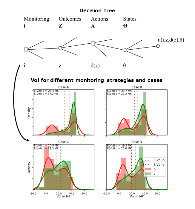
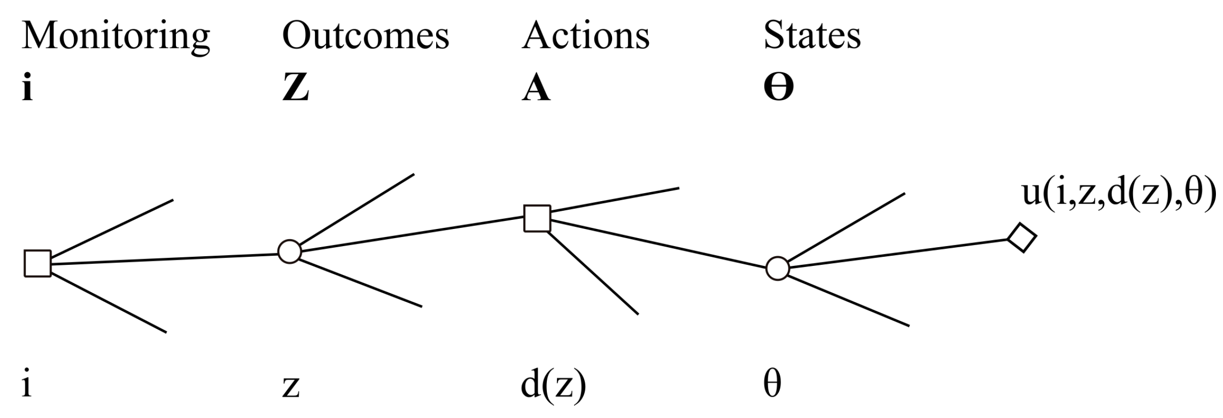
Bayesian decision models are based upon an important distinction between the state of a system and the belief of a decision maker about that state and were first introduced by [10]. These models support decisions by translating sets of actions for acquiring information, and actions following from this information, into estimates for utility. The general goal of such models is to assess the value of certain information in a particular decision problem. A general formulation of such a model is given in Figure 1. The decision tree presented here consists of four levels:

• The action to acquire information $i\in I$, where I is the set of all possible information acquiring actions.
• The outcome of the action to acquire information, $z\in Z$, where Z is the set of all possible outcomes. Note that z is used to update the belief of the decision maker about the state $\theta$ (see the last bullet).
• The action $a\in A$ following the obtained information, where A is the set of all possible actions. Here, it should be noted that this can be formulated by a decision rule which maps different outcomes $a\in A$ to outcomes $z\in Z$. This yields a decision rule $d\left(z\right)$ that assigns an a to each z. Hence, we use a set of decision rules $d\left(z\right)\in A$.
• The state of nature $\theta \in \Theta$ where $\Theta$ is the a priori set of all possible states of nature.

Based on the input values for the different levels of the decision tree, one can compute a utility $u(i,z,d(z),\theta )$ for each combination of information and action (i and $d\left(z\right)$) and realization for the state of nature $\theta$. However, typically we do not know the outcome z of a yet to be obtained information, and here Bayesian pre-posterior decision analysis provides a structured framework to evaluate combinations of $i\in I$ and $d\left(z\right)\in D\left(z\right)$ and obtain the optimal combination based on the a priori information using [11]:

$$u(i,d\left(z\right))=\underset{i\in I,d\left(z\right)\in D\left(z\right)}{max}{E}_{\Theta }\left[E_{z|\Theta }\left[u(i,z,d\left(z\right),\Theta )\right]\right]),$$

(1)

where $D\left(z\right)$ is the set of possible decision rules and $\Theta$ is the prior distribution of state of nature. By comparing this utility to the utility without information i:

$$u\left(d\left(z\right)\right)=\underset{d\left(z\right)\in D\left(z\right)}{max}{E}_{\Theta }\left[u(d\left(z\right),\Theta )\right]),$$

(2)

one can obtain the Value of Information of the action to acquire information i:

$$VoI=u(i,d(z\left)\right)-u\left(d\right(z\left)\right).$$

(3)

Various studies on inspection and Structural Health Monitoring decision trees such as the one in Figure 1 have been extended with additional levels (see, e.g., [11,33]). While decision trees are insightful, they have as a disadvantage that they grow exponentially when multiple sequential decisions are considered [10]. As an analysis of an asset management strategy for 100–200 years consists of multiple sequential and dependent decisions (i.e., a decision in $t+1$ should account for findings at t), simply repeating a decision tree is not practical for this type of problem. Sequential decision problems can be solved by defining policies or strategies, which are sets of decision rules that indicate what action has to be taken under which circumstances at which time step t [11,26,34]. An example is an inspection strategy where an inspection is carried out at interval $\delta t$, possibly followed by a repair given that some parameter $X<x$. The disadvantage of using policies is that it might not yield an optimal solution, although it was found by [35] that the solution can be close to that obtained with other methods that are capable of finding an optimal solution, provided that the heuristics are well formulated. Such a heuristic approach can be combined with any type of time-dependent (Bayesian) decision model [34]. In this study, we use a Bayesian decision model based on First Order Reliability Method calculations for the flood defence reliability in each year. This approach will be further outlined in Section 3.

As our main aim is to examine pore pressure monitoring for various types of flood defences, there is a significant number of parameters that can be varied in order to obtain a policy. Of specific importance is that the outcome of a monitoring action is uncertain as the information obtained depends on the extremity of the observed water levels. Typically, more extreme observations lead to more information [23]. 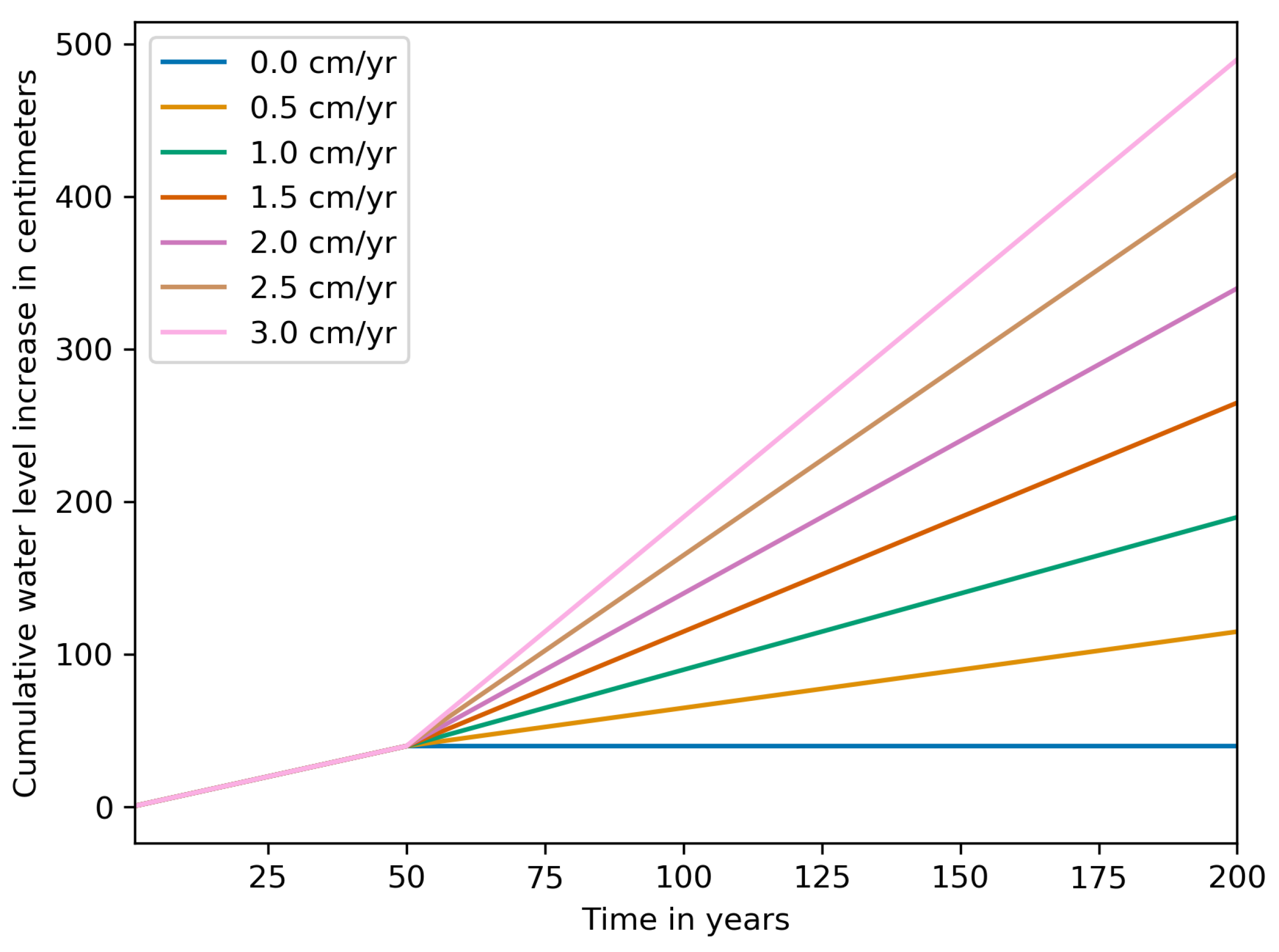Thus, the VoI of a single monitoring action is also uncertain, and dependent on the duration of the action and observed hydraulic loads—or in general terms: even if an action to acquire information i is carried out at year t, it depends on the observed water levels whether observation z can be used to update the belief. In addition, there is considerable uncertainty in future developments, particularly the impact of climate change. Current sea level rise scenarios for the Netherlands range between +0.5 and +3.0 m for the end of the century [36]. If sea level rise is much higher than anticipated, this will dictate the investment pattern for future reinforcements. In such a case, while SHM outcomes might be favourable, the service life extension will be negligible (i.e., a reinforcement is needed in any case), meaning that the VoI of pore pressure monitoring might be reduced for high rates of sea level rise. To obtain insights in the VoI, given different rates of future sea level rise, we analyse the VoI conditional on different rates.

3. Methodology

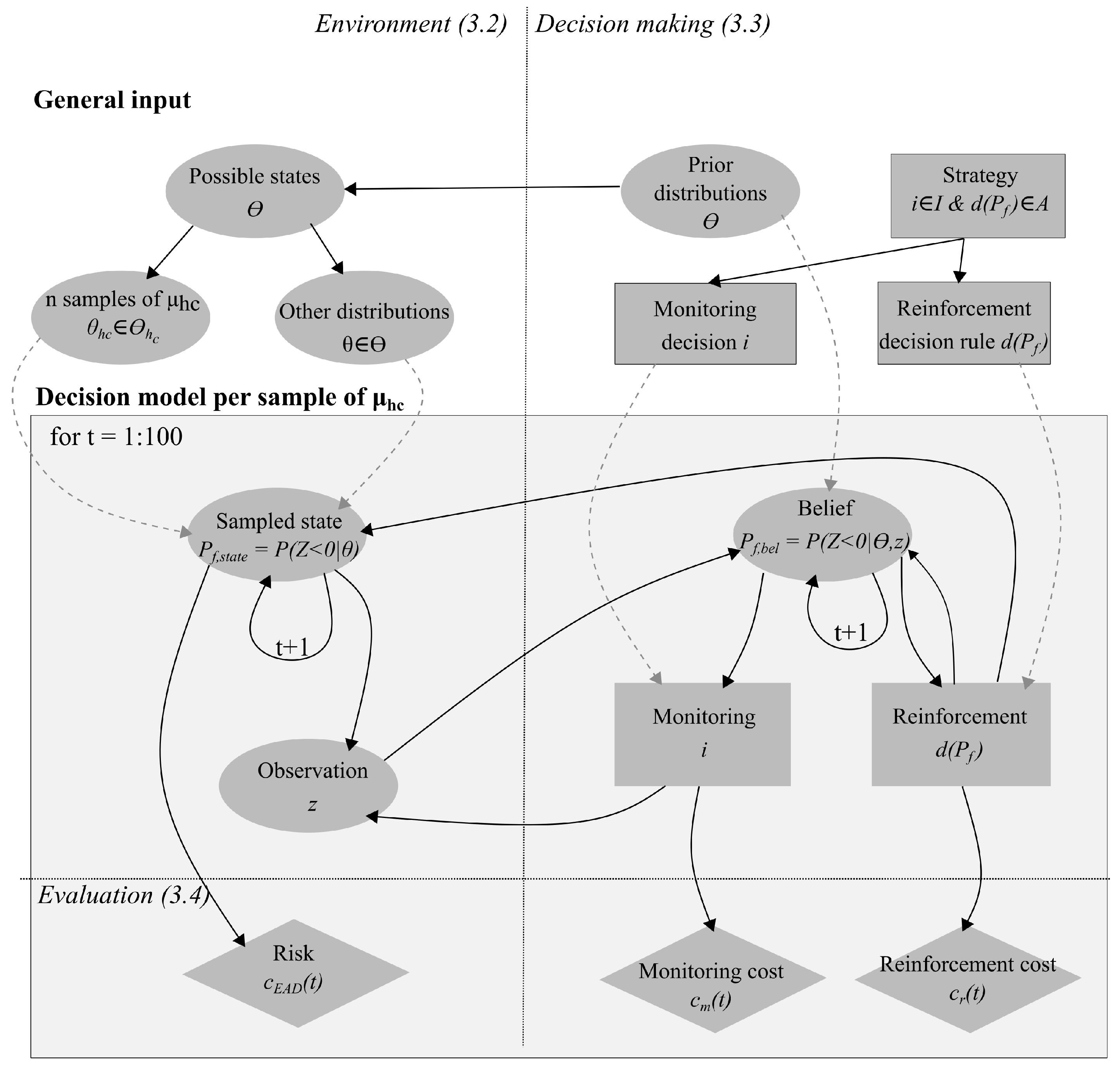
In this paper, a pre-posterior Bayesian decision model is used to derive the cost and VoI of different monitoring strategies for different possible posterior states. These states are a description of the system, should all epistemic uncertainties be reduced. Strategies are defined as sets of heuristic policy rules, and contain all activities taken during the considered time period. Figure 2 gives an overview of the methodology, including the subsections in which each part is discussed in more detail. The figure consists of two main parts: the top part concerns how input is derived for runs of the Bayesian decision model. An influence diagram that represents the Bayesian decision model is shown in the bottom part. For most blocks in the diagram, parameters are given that relate to the parameters in Figure 1. It has to be noted that, in this model, observations z are translated to posterior failure probabilities ($P(Z<0|\Theta ,z$), while, in Figure 1, z was directly translated to actions through decision rule $d\left(z\right)$. Several strategies are evaluated using a set of sampled possible posterior states that are consistent with the prior beliefs. As the failure model is important for all other sections, its general set-up is discussed first in Section 3.1. Next, Section 3.2 describes how prior distributions $\Theta$ are translated to samples of posterior states of the system $\theta$ and observations z; this concerns the left part of the figure (left of the dotted line). Section 3.3 deals with the right part of the figure, most notably how heuristic decision rules for monitoring and reinforcement (i and $d\left(P\mathrm{f}\right)$) are used to update $P_{\mathrm{f}},\mathrm{state}$ and $P_{\mathrm{f}},\mathrm{bel}$. In Section 3.4, how the utility for each run can be translated to estimates for the cost and Value of Information is discussed.

3.1. Time-Dependent Failure Probability Model

While in the decision tree in Figure 1 the state of the observed variable could be translated to utility directly, in our case, the utility depends on the failure probability of the flood defence. Hence, we have to translate observations (z in the decision tree) to a failure probability. In the decision model, we assess the performance of the flood defence by means of a fragility curve [37]. A fragility curve denotes the probability of failure given a realization of some parameter; for flood defences, typically the water level h is used, so $P_{\mathrm{f}}|\mathrm{h}$. For the simple limit state function $Z=h_{\mathrm{c}}-h$, with $h_{\mathrm{c}}$ the critical water level (at which failure occurs) (in m +ref) and h the water level [in m +ref] and $Z<0$ denotes failure, it holds that:

$$P_{\mathrm{f}}=P(Z<0)=P(h>h_{\mathrm{c}})={\int }_{h}P(h>h_{\mathrm{c}}|h)·f_{\mathrm{h}}\left(h\right)\mathrm{d}h={\int }_h{F}_{h_{\mathrm{c}}}\left(h\right)·f_{\mathrm{h}}\left(h\right)\mathrm{d}h,$$

(4)

where $P_f$ is the annual failure probability for the flood defence section considered. We assume that the uncertainty in h is fully aleatory and has irreducible meaning that no measure is available to reduce this uncertainty.

Over time, both $h_{\mathrm{c}}$ and h will change due to, respectively, deterioration (e.g., settlement) and climate change induced increase in extreme water levels. The time-dependent limit state function is then described by:

$$Z\left(t\right)=[h_{\mathrm{c}}\left(t\right)-\Delta h_{\mathrm{c}}\left(t\right)]-[h+\Delta h\left(t\right)],$$

(5)

where $\Delta h_{\mathrm{c}}\left(t\right)$ and $\Delta h\left(t\right)$ denote the deterioration, respectively, water level increase in meters. In our decision problem, we consider the Value of Information from pore pressure monitoring. Pore pressure monitoring would reduce a part of the uncertainty in $h_{\mathrm{c}}$(t). Hence, within the constraints of our decision problem, we consider all other uncertainties to be irreducible. It has to be noted that, in [26], uncertainty reduction in $\Delta h_{\mathrm{c}}\left(t\right)$ and $\Delta h\left(t\right)$ was also considered. For $\Delta h_{\mathrm{c}}\left(t\right),$ this was found to have a very limited effect, whereas $\Delta h\left(t\right)$ is better dealt with using Value of Information conditional on different scenarios for $\Delta h\left(t\right)$. Both are considered to be deterministic in evaluations of this Bayesian decision model in Section 5.1; in Section 5.2, we will consider multiple scenarios for $\Delta h\left(t\right)$.

While pore pressure monitoring can reduce a part of the uncertainty in $h_{\mathrm{c}}$(t), there is also an irreducible part. It should be noted that this part is irreducible by pore pressure monitoring, but there might be other methods to reduce this uncertainty. However, we do not consider these in our decision problem. We can describe the uncertainty in $h_{\mathrm{c}}$ as follows:

$$\begin{array}{cc}\hfill h_{\mathrm{c}}\sim & N({\mu }_{\mathrm{h}}\mathrm{c},{\sigma }_{\mathrm{irr}}),\hfill \end{array}$$

(6)

$$\begin{array}{cc}\hfill {\mu }_{{\mathrm{h}}_{\mathrm{c}}}\sim & N(\mu ,\sigma ),\hfill \end{array}$$

(7)

where ${\mu }_{{\mathrm{h}}_{\mathrm{c}}}$ denotes the mean of a possible state of the flood defence. ${\sigma }_{\mathrm{irr}}$ denotes the part of the uncertainty that is irreducible in the decision problem. How this definition is translated into values for $P_{\mathrm{f}},\mathrm{state}$ and $P_{\mathrm{f}},\mathrm{bel}$ is discussed in the following sections.

3.2. Environment

3.2.1. General Input

The environment describes the state space of the flood defence that consists of all sampled posterior states ($\theta \in \Theta$ in the decision tree). 5 shows that there are four random variables in the Limit State Function that determine this state. In our analysis, we only consider observations of parameter $h_{\mathrm{c}}$. Based on our prior belief (${\Theta }_{\mathrm{h}}\mathrm{c}$), there are many possible posterior states for parameter $h_{\mathrm{c}}$ in Figure 1), which is reflected by the fact that ${\mu }_{{\mathrm{h}}_{\mathrm{c}}}$ is normally distributed with mean $\mu$ and standard deviation $\sigma$ (see Equation (7)). This distribution of ${\mu }_{{\mathrm{h}}_{\mathrm{c}}}$ reflects the epistemic uncertainty of our state space [10]. Thus, it holds that:

$$\begin{array}{cc}\hfill {\Theta }_{\mathrm{h}}\mathrm{c}\sim N(N(\mu ,\sigma ),{\sigma }_{\mathrm{irr}})& ,\hfill \end{array}$$

(8)

$$\begin{array}{cc}\hfill {\theta }_{\mathrm{h}}\mathrm{c},\mathrm{j}\sim N({\mu }_{\mathrm{j}},{\sigma }_{\mathrm{irr}})& \mathrm{with} j=1,2,\dots ,n,\hfill \end{array}$$

(9)

where n is the number of samples drawn from ${\mu }_{{\mathrm{h}}_{\mathrm{c}}}$ (Equation (7)) and ${\theta }_{\mathrm{h}}\mathrm{c},\mathrm{j}$ is the j^th sample of a possible posterior state.

For the variables governed by a temporal process ($\Delta h_{\mathrm{c}}\left(t\right)$ and $\Delta h\left(t\right)$), we use deterministic variables for the rate. In reality, both variables will contain at least some uncertainty, but it was shown by [26] that reducing uncertainty in $\Delta h_{\mathrm{c}}\left(t\right)$ has little influence on decisions. For $\Delta h\left(t\right)$, some recent scenarios show that sea level rise in 2100 might range between 0.5 and 3 m [36], although this has been nuanced by [38]. In the pre-posterior analysis, we do not include this uncertainty such that the effect of monitoring of $h_{\mathrm{c}}$ is more clear from the results. Thus, the prior distribution is a deterministic distribution with a certain annual rate $\Delta h\left(t\right)$. To assess the effect of different future rates of $\Delta h\left(t\right),$ we analyse the Value of Information conditional upon $\Delta h\left(t\right)$. Thus, for each possible value, a separate pre-posterior analysis will be carried out. This will be discussed further in Section 5.2.

3.2.2. Decision Model

For every time step, 5 is re-evaluated in order to account for the temporally changing variables. Thus, for every time step, a failure probability $P_{\mathrm{f}},\mathrm{state}=P(Z<0|\theta )$ is computed. A reinforcement decision might incrementally change the belief of $h_{\mathrm{c}}$ for the next time step. For strategies where monitoring equipment is installed, an observation of $h_{\mathrm{c}}$ is sampled from the state.

3.3. Decision-Making

3.3.1. General Input

Decisions are defined using strategies consisting of heuristic decision rules $S_{\mathrm{j}}$. A heuristic rule typically has the form: if some_variable is larger than some_threshold, we take some_action. The model contains decision rules for monitoring and reinforcement. We consider three different sets of decision rules for monitoring ($i\in I$ in Figure 1):

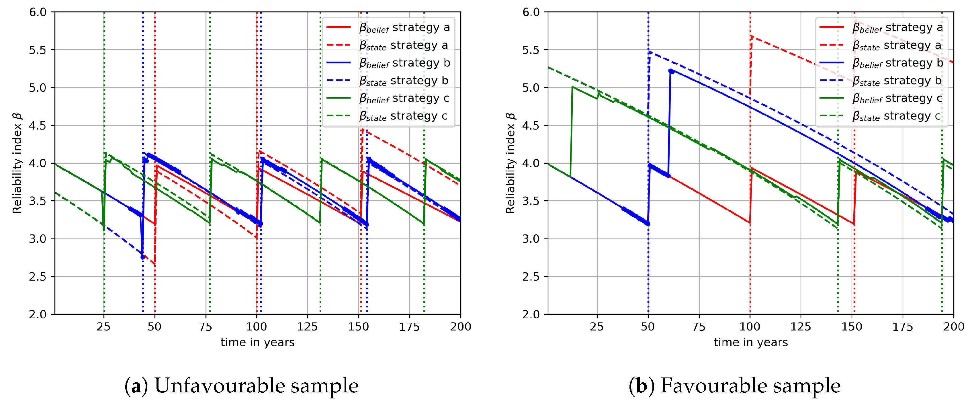
• Strategy a: no monitoring.
• Strategy b: monitoring is started if the failure probability $P_{\mathrm{f}},\mathrm{bel}>0.5·P_{\mathrm{req}}$, where $P_{\mathrm{req}}$ is the reliability requirement. Monitoring is stopped after 25 years.
• Strategy c: continuous monitoring starting at $t=1$.

For reinforcement decisions, the same rules are used in all calculations: if $P_{\mathrm{f}},\mathrm{bel}\left(t\right)<P_{\mathrm{req}}$, a flood defence is reinforced such that $P_{\mathrm{f}},\mathrm{bel}(t+t_{\mathrm{design}})=P_{\mathrm{req}}$. Here, $t_{\mathrm{design}}$ is the design period of the flood defence. In terms of the decision tree in Figure 1, this means that we have only one set of $d\left(P_{\mathrm{f}}\right)\in A$, which is identical for all t.

3.3.2. Decision Model

In order to obtain pre-posterior estimates for the cost of each strategy, we evaluate a set of possible posterior states j. For each sampled posterior state j (see ), the belief estimate of the reliability ($P_{\mathrm{f}},\mathrm{bel}\left(t\right)=P(Z<0|\Theta ,z\left(t\right))$ in the decision model is recalculated for every time step in order to account for the temporally changing variables and reinforcement decisions. Additionally, observations from monitoring can result in an updated belief using the observations from monitoring up to time t, $z\left(t\right)$. The initial belief of $h_{\mathrm{c}}$ is defined as: ${\Theta }_{\mathrm{h}}\mathrm{c}\sim N(N(\mu ,\sigma ),{\sigma }_{\mathrm{irr}})$.

If monitoring equipment is present, an observation of the state might be made, depending on the extremity of the observed circumstances, while, in [23], it was found that more extreme circumstances gradually increase the VoI; here, we use a discrete threshold value to distinguish between years with and without useful observation. Whether an observation at $t=i$ is useful is determined by the following condition:

$$P(h_{\mathrm{i}}>H)<P_{\mathrm{thresh}},$$

(10)

where $P(h_{\mathrm{i}}>H)$ is the annual exceedance probability of a randomly sampled water level $h_{\mathrm{i}}$, and $P_{\mathrm{thresh}}$ is a predefined threshold value that has to be exceeded for an observation to be useful for updating the belief of $h_{\mathrm{c}}$. Analogous to a Probability of Detection for inspections, this can be interpreted as a Probability of Observation [11,33]. As both prior and posterior of $h_{\mathrm{c}}$ are normally distributed, the conjugate distributions can be used to obtain the posterior distribution at time t, $h_{\mathrm{c}}|z\left(t\right)$ [10]:

$$h_{\mathrm{c}}|z\left(t\right)\sim N(\frac{n\overline{z}}{n^{\prime }+n},\sqrt{\frac{{\sigma }_{\mathrm{irr}}^2}{n^{\prime }+n}+{\sigma }_{\mathrm{irr}}^2}),$$

(11)

where the prior weight is given by $n^{\prime }={\sigma }_{\mathrm{irr}}^2/{\sigma }^{\prime }$ with ${\sigma }^{\prime }=\sqrt{{\sigma }^2-{\sigma }_{\mathrm{irr}}^2}$, n is the number of observations obtained until t, and $\overline{z}=\sum \left(z\left(t\right)\right)/n$ is the mean of the observations up to t. The observations are random samples from the considered state ${\theta }_{\mathrm{h}}\mathrm{c},\mathrm{j}$ (see Equation (9)). The effect of this approach is that, for longer periods of monitoring, the expected number of useful observations will increase. In addition, for a short period of monitoring, the number of useful observations can vary, and there might not be any information obtained at all.

A reinforcement is carried out if the flood defence no longer meets the required minimum annual failure probability requirement $P_{\mathrm{req}}$. In such a case, the mean $\mu$ of $h_{\mathrm{c}}$ is iteratively increased such that it holds for the belief of $h_{\mathrm{c}}$ that:

$$P(Z(t+t_{\mathrm{design}})<0)>P_{\mathrm{req}},$$

(12)

where $t_{\mathrm{design}}$ is the design period in years. In case of a reinforcement, the coefficient of variation of the belief of $h_{\mathrm{c}}$ is assumed to be the same before and after reinforcement.

3.4. Evaluation

For each evaluation of a strategy for a sampled possible state $\theta$, three discounted cost components are computed for the evaluated period of n years: the Expected Annual Damage (EAD) due to flooding or risk costs ($C_{\mathrm{EAD}}$), the cost of monitoring equipment ($C_{\mathrm{m}}$) and cost of dike reinforcement ($C_{\mathrm{r}}$). The overall discounted cost of a strategy for a sample $\theta \in \Theta$ over a period of n years can be written as:

$$c_{\mathrm{s}|\theta }=C_{\mathrm{EAD}}+C_{\mathrm{m}}+C_{\mathrm{r}}=\sum _t^n\frac{c_{\mathrm{EAD}}\left(t\right)+c_{\mathrm{m}}\left(t\right)+c_{\mathrm{r}}\left(t\right)}{{(1+r)}^t},$$

(13)

where $c_{\mathrm{EAD}}\left(t\right)$ is the cost component of the EAD at time t and $c_{\mathrm{m}}\left(t\right)$ and $c_{\mathrm{r}}\left(t\right)$ are the costs for monitoring and reinforcement at time t. Note that these are equal to 0 if no reinforcement or monitoring is done at a specific time step t. r is the discount rate, for which a value of $3\%$ is prescribed in the Netherlands.

In this paper, we study the Value of Information (VoI) of different asset management strategies based on their performance over a time span of 200 years. If we consider a strategy $s_{\mathrm{j}}$ where information is acquired, the $VoI$ can be calculated as the difference in expected costs based on all samples $\theta$ with the expected costs of baseline strategy a ($E\left(c_{\mathrm{a}}\right)$):

$$\begin{array}{cc}\hfill VoI\left(s_{\mathrm{j}}\right)& =E\left(c_{\mathrm{a}}\right)-E\left(c_{s_{\mathrm{j}}}\right)with:\hfill \end{array}$$

(14)

$$\begin{array}{cc}\hfill E\left(c_{s_{\mathrm{j}}}\right)& =\frac{{\sum }_N{c}_{s_{\mathrm{j}}|\theta }}{N},\hfill \end{array}$$

(15)

where $VoI\left(s_{\mathrm{j}}\right)$ is the Value of Information for strategy $s_{\mathrm{j}}$ and N is the number of samples of $\theta$ that are considered.

If a $VoI$ is conditional upon a value for an observed parameter (in our case $h_{\mathrm{c}}$), it is defined as a conditional Value of Information ($cVoI$) or option value [10,39]. This can be used to assess the $VoI$ given the possible outcomes of monitoring (e.g., the VoI given $\theta$ or z). To assess the influence of future uncertainty on the Value of Information, we use a slightly modified formulation of this concept in Section 5.2. Here, we do not formulate the VoI conditional on the monitored parameter itself ($h_{\mathrm{c}}$), but rather on a different model parameter, namely the value for the change in water level $\Delta h=h_{\mathrm{j}}$. Thus, the $cVoI$ for a strategy $s_{\mathrm{j}}$ can be obtained using the following equation:

$$cVoI\left(s_{\mathrm{j}}\right|\Delta h=h_{\mathrm{j}})=E\left(c_{\mathrm{A}}(\Delta h=h_{\mathrm{j}})\right)-E\left(c_{s_{\mathrm{j}}}(\Delta h=h_{\mathrm{j}})\right).$$

(16)

It has to be noted that this $cVoI$ is formulated differently than the conditional Value of Information concept given by [10].

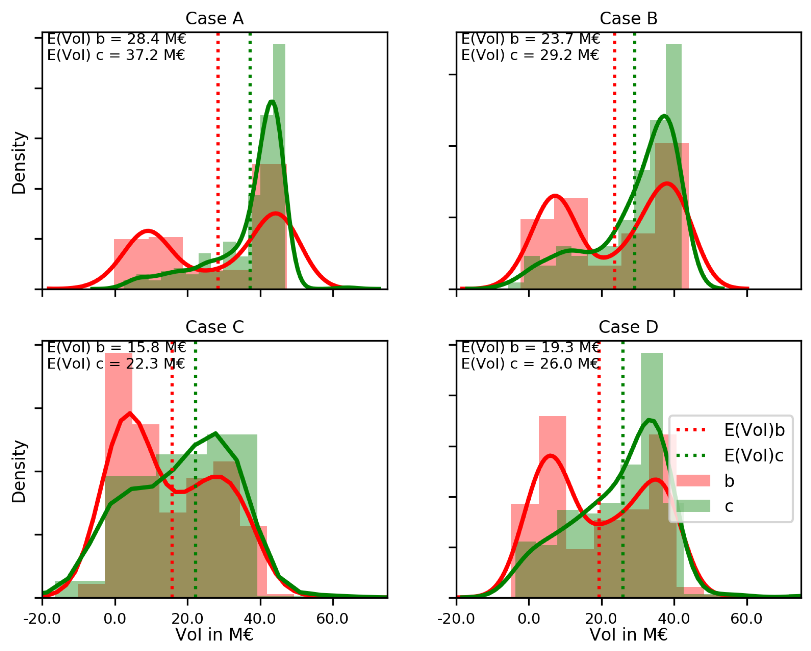
4. Case Study

In order to determine the VoI of pore pressure monitoring, we consider a set of parameterized cases, based on values obtained in actual probabilistic assessments such as VNK2 [29]. Each case is obtained by modifying input distributions such that the initial reliability index $\beta$ is around 4 (with $\beta =-{\Phi }^{-1}\left(P_{\mathrm{f}}\right)$). We parameterize in two ways: first, we consider different sets of the $\alpha$ influence coefficients in the design point obtained from FORM calculations. A high $\alpha$ influence coefficient indicates that the uncertainty in a parameter has a major influence on the obtained reliability index $\beta$ [40]. From probabilistic calculations throughout the Netherlands, it is found that, for instance, for the failure mode piping erosion, the ${\alpha }^2$ of the strength can vary between 0.1 and 0.9. Additionally, we vary the extent to which the uncertainty in the strength is epistemic and reducible. The highest VoI is expected to be encountered for cases with a large $\alpha$ of the strength, of which a major part is epistemic.

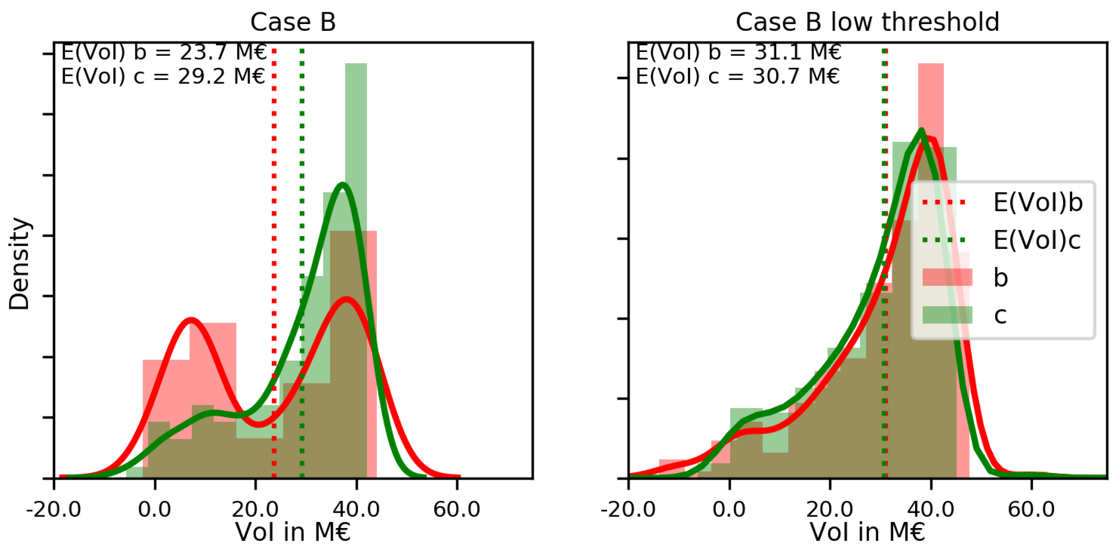
Additionally, we consider two different threshold values at which an observation can be made ($P_{\mathrm{thresh}}$). The default threshold represents a flood defence at a lowland river with larger floodplains bounded by summer dikes. Hence, one would expect a relatively high threshold ($P_{\mathrm{thresh}}=1/10{\mathrm{year}}^{-1}$) in 10, as water has to overflow the summer dike before obtaining a measurement. We also consider a lower threshold which represents a location without summer dikes in a delta region relatively close to the sea ($P_{\mathrm{thresh}}=1/2{\mathrm{year}}^{-1}$).

For the costs of reinforcement, the relation for dike ring 16 given in [41] is used, with which the exponentially increasing costs of an incremental increase in $h_c$ can be obtained. The costs for installing monitoring equipment are assumed to be €200,000. All other input values as well as prior design point values are shown in

Table 1. All input data for cases A, B, C and D. The top part shows all input distributions, the middle part shows the initial design point values for the influence of the strength uncertainty and epistemic part of the strength uncertainty, as well as the prior reliability index ${\beta }_{\mathrm{prior}}$. The bottom part shows the threshold $P_{\mathrm{thresh}}$ for the normal case and a lower threshold, safety standard $P_{\mathrm{norm}}$, planning period $t_{\mathrm{plan}}$ and discount rate r for each case.

	Name	Unit	Distribution		Case
			Type	Values	A	B	C	D
Input distributions	${\mu }_{\mathrm{h}}\mathrm{c}$	m +ref	Normal	$\mu$	7.56	6.12	5.76	5.88
				$\sigma$	1.03	0.58	0.42	0.50
				${\sigma }_{\mathrm{irr}}$	0.2	0.2	0.2	0.2
	h	m +ref	Gumbel	a	3.2
				b	0.2
	$\Delta h$	mm/yr	Determ.		8
	$\Delta h_{\mathrm{c}}$	mm/yr	Determ.		5
Initial design point	${\beta }_{\mathrm{prior}}$	-			3.96	4.00	4.01	4.03
	${\alpha }_{\mathrm{h}}{\mathrm{c}}^2$	-			0.74	0.57	0.34	0.41
	${\alpha }_{{\mu }_{\mathrm{h}}\mathrm{c}}^2$	-			0.69	0.51	0.28	0.39
Other input	$P_{\mathrm{thresh}}$	-/yr			Default: 0.1 Lower: 0.5
	$P_{\mathrm{norm}}$	-/yr			1/3000
	$t_{\mathrm{plan}}$	yr			50
	r	%/yr			3

.

For each considered case, 250 different posterior states are sampled from the state space. In some cases, samples are drawn from the state space that have a very low reliability after 50 years ($\beta <2$) and have a probability smaller than $1/N$, where N is the sample set. Such samples result in extremely high risk costs that dominate the Total Cost computation. Therefore, all samples where $\beta (t=50)<2$ are removed from the state space; other approaches to cope with this will be discussed in Section 6.

5. Results

5.1. Benefits of Monitoring for a Deterministic Future

Our first analysis concerns the benefits of monitoring without uncertainty in future development (temporal changes in load and resistance are deterministic). In order to better understand the way individual samples of posterior states $\theta$ are dealt with, we examine the influence of monitoring on the reliability $\beta$ in time for two sampled posterior states for Case B. This is shown in Figure 3. Figure 3a shows a relatively unfavourable sample of ${\mu }_{{\mathrm{h}}_{\mathrm{c}}}$, which means that the posterior reliability after obtaining observations is lower than the prior estimate. Figure 3b shows a favourable sample; here, the posterior reliability is higher than the prior. For each strategy, two computations of $\beta$ are shown: one for the sampled posterior state ${\beta }_{\mathrm{state}}$, this indicates the reliability should all epistemic knowledge be reduced. A second line is shown for the development of the decision makers’ belief over time ${\beta }_{\mathrm{belief}}$. The left pane shows that, in strategies with monitoring (b and c), reinforcement is done earlier than without monitoring, provided that observations are obtained which confirm the unfavourable ${\mu }_{{\mathrm{h}}_{\mathrm{c}}}$. Hence, life-cycle costs will be higher with monitoring, but risk costs will be lower. In Figure 3b, the sampled ${\mu }_{{\mathrm{h}}_{\mathrm{c}}}$ is much more favourable and, for strategy c, reinforcement is postponed by about 85 years. For strategy b, the reinforcement is not postponed, as there is no useful observation in the first 20 years of monitoring (indicated by the line marked with circles). However, in the entire sample set, there are realizations with a similar ${\theta }_{\mathrm{h}}\mathrm{c}$, where there are observations and the reinforcement is also postponed for strategy b. The ratio between cases with and without postponed investment depends on the value of $P_{\mathrm{thresh}}$.

This is shown on a more general level by Figure 4. Here, the VoI for strategies b and c compared to reference strategy a is represented by a (Gaussian) kernel density estimation (KDE). It can be observed that for strategy b (in red) there are two peaks in density, whereas for strategy c there is only one peak. As the first reinforcement is after about 50 years, for strategy c, the probability of not having any useful observation before that time is quite small (about $1/200$). As strategy b only monitors for a limited amount of time, this probability is much larger (about 30%), thus two modes are found in the KDE estimation for each case. The left mode corresponds to cases where the first reinforcement is not postponed, either because observations have not been obtained, or because the posterior strength is still insufficient. The right mode corresponds to cases where it is postponed. This difference illustrates how important it is to include the uncertainty on whether an observation will be obtained during the envisaged monitoring period. The influence on subsequent reinforcements is not clearly visible from the KDE estimates, as the life-cycle costs are significantly lower due to discounting.

Theoretically, it is expected that $E\left(VoI\right)$ decreases if the relative contribution of reducible uncertainty in ${\mu }_{{\mathrm{h}}_{\mathrm{c}}}$ decreases. In Figure 4, we can see that this is indeed the case: cases with a lower influence coefficient of reducible uncertainty in the strength ${\alpha }_{{\mu }_{\mathrm{h}}\mathrm{c}}$ have a lower E(VoI). Figure 5 shows this more clearly, also for an additional case where ${\alpha }_{{\mu }_{\mathrm{h}}\mathrm{c}}$ is even smaller. From this figure, we see that the $E\left(VoI\right)$ clearly increases with larger influence of epistemic uncertainty.

In relative terms, it is important to note that the Total Cost for all cases is on average in the order of 50–60 M€, where it is low for most samples, but the average is strongly influenced by cases where the flood defence strength is more unfavourable than expected, and the risk costs are above the a priori estimate. It is found that on average the Total Cost for strategy b is between 40% and 70% of the reference strategy a, and for strategy b between 25% and 60%.

It was shown before that monitoring benefits strongly depend on the duration of monitoring and the probability of having a useful measurement before the next major investment decision. Hence, we compare case B with an identical case where it holds that $P_{\mathrm{thresh}}=1/2{\mathrm{year}}^{-1}$ rather than the default value $P_{\mathrm{thresh}}=1/10{\mathrm{year}}^{-1}$. We would expect the left density peak to be significantly smaller for strategy b in case B with a lowered threshold. Say that there are 10 years before the planned reinforcement, the probability of having no useful observation for a lower threshold compared to the default case B is a factor

$$\frac{P\left(\overline{\mathrm{B}}\right)}{P\left(\overline{\mathrm{B}\mathrm{low}\mathrm{threshold}}\right)}=\frac{{(1-P_{\mathrm{thresh}})}^t}{{(1-P_{\mathrm{thresh}},\mathrm{lower})}^t}=\frac{{(1-0.1)}^{10}}{{(1-0.5)}^{10}}\approx 357$$

(17)

smaller, where $P\left(\overline{\mathrm{B}}\right)$ is the probability of having no observation, for case B, and t is the period up to the next major decision. Figure 6 shows KDE-estimates for both cases. Here, it can be observed that, for case B with a lower threshold, there are no longer two peaks in density for strategy b (in red): KDE-estimates are very much alike for both strategies b and c. This illustrates the importance of including the relation between monitoring duration and expected (number of) observations.

5.2. The Effect of Future Uncertainty on the Value of Information of Monitoring

In the previous section, we assumed deterministic changes of load and resistance. However, in reality, especially the future development of the load is very uncertain, amongst others due to sea level rise (SLR) and changing hydrological conditions. Contributing factors such as Antarctic ice sheet mass loss might or might not result in an increasing acceleration of global sea level rise, for which high-end estimates are in the order of 3 m by the end of the 21st century [36,42]. Recent publications have argued that these estimates are likely too high but that there are many remaining uncertainties towards the precise contribution of ice sheet mass loss to sea level rise [38]. Studies on sea level rise observations have found some indication of acceleration from satellite observations [43], whereas others have not found this from tidal gauges [44,45]. For river discharges, the effects of a changing climate vary per region, but there are several examples of catchments where discharges, and thus water levels, are expected to increase [46]. Given the large uncertainty that exists, it is of interest to identify actions that are beneficial in a wide variety of future scenarios.

In the context of this paper, the exact rate of water level increase is not directly of interest to the question whether SHM should be used to reduce epistemic uncertainties, but rather the question of whether the Value of Information is sensitive to the range of possible future scenarios. Hence, in this section, we explore whether an investment, in efforts to reduce epistemic uncertainties, is robust in the sense that the VoI is positive for the entire range of possible rates of water level increase.

In this section, we explore this for Case B from the preceding section, which has a commonly encountered value for influence coefficient ${\alpha }_{h_{\mathrm{c}}}$. We consider a range of scenarios with increases in water levels $\Delta h\left(t\right)$ between 0 and 3 cm per year, in line with the ranges given by [36,47]. We assume that $\Delta h\left(t\right)$ changes from the original value to the scenario rate at $t=50$ years; this is shown in Figure 7.

Figure 8a shows the Conditional VoI given different rates of $\Delta h\left(t\right)$. Here, we see that the VoI increases for both strategies b and c for higher rates of water level increase. In Figure 8b, the ratio of the Total Costs with and without monitoring is shown for the different scenarios, including 5/95% upper and lower bounds. This ratio is quite stable, as aside from the increase in VoI, also the total investment costs increase significantly as there are more reinforcements needed to maintain the reliability requirement. In addition, the overall uncertainty reduces slightly for more extreme rates of water level increase. This is explained by the fact that the two modes observed in the KDE estimates disappear for high rates of water level increase (see Figure A1). This is caused by the fact that the total cost is not completely dominated by the first reinforcement, but also by the number of consecutive reinforcements which increases for high rates of water level increase. Hence, the KDE estimates become smoother for more extreme changes.

6. Discussion

Probabilistic calculations of flood defence reliability often show that strength uncertainties have a major influence on flood defence reliability estimates. In practice, reduction of such uncertainties often results in a major change in such estimate [23,24,48], leading towards different reinforcement and maintenance decisions. The general aim of this paper is to show in what circumstances reduction of epistemic strength uncertainty improves asset management decisions for flood defences, focusing on long-term reinforcement investments. We paid specific attention to the fact that often monitoring results depend on observed loads.

There are various ways in which the influence of epistemic uncertainty on reliability estimates can be reduced, most notably the inclusion of survival observations in general due to correlation of resistance parameters in time [49], survival of past extreme events [48,50] or actively reducing uncertainties by monitoring or site investigation. The latter has been investigated in this paper, and neither of the former two are considered in the computations. This means that all failure probabilities that are computed are not conditional on previous years. In [49], it was shown that, especially for lower reliability indices and high temporal correlation of the resistance, conditional reliability estimates were significantly higher. Therefore, in this paper, we might slightly overestimate the VoI of Case A. For other cases, this will be less of an issue as the difference between conditional and unconditional reliability estimates is much smaller.

In this paper, we have defined the dike strength using general fragility curves rather than a specific failure mechanism. The reason is that the aim of this paper is to give insight in the relative influence of reducible and irreducible uncertainty on monitoring benefits, rather than elaborate this for a specific mechanism. Pore pressure monitoring is used as illustration since this is one of the most commonly applied monitoring techniques for earthen flood defences. The general principle is valid for any monitoring method for which the obtained information is dependent on observed loads. For the relative influence of uncertainties, we derived a set of cases based on existing flood defence reliability assessments. In principle, it is possible to do the analysis for specific cases with specific failure mechanisms and other monitoring methods, as was already illustrated in [23]. This would also allow for better accounting for measurement uncertainty.

Often, VoI analysis is based upon investment cost reduction only, whereas here we have also included the risk costs. This is particularly important as risk costs increase exponentially with an increase in failure probability when the resistance is lower than expected. Hence, monitoring has two potential benefits: reducing risk for unfavourable posterior outcomes and reducing investment costs for favourable posterior outcomes. In line with what is experienced in practice, in most of the cases, the posterior after monitoring is favourable. A point of attention towards the approach used is that some samples contain posterior states that have very high failure probabilities. In such cases, the risk exponentially increases, resulting in single samples that have a very large influence on the VoI estimates. As these specific samples are often unrealistic, all samples for which $\beta (t=50)<2$ have been excluded. Potentially, more elegant solutions to this are including survival observations or conditional failure probabilities, which will likely result in the same effect.

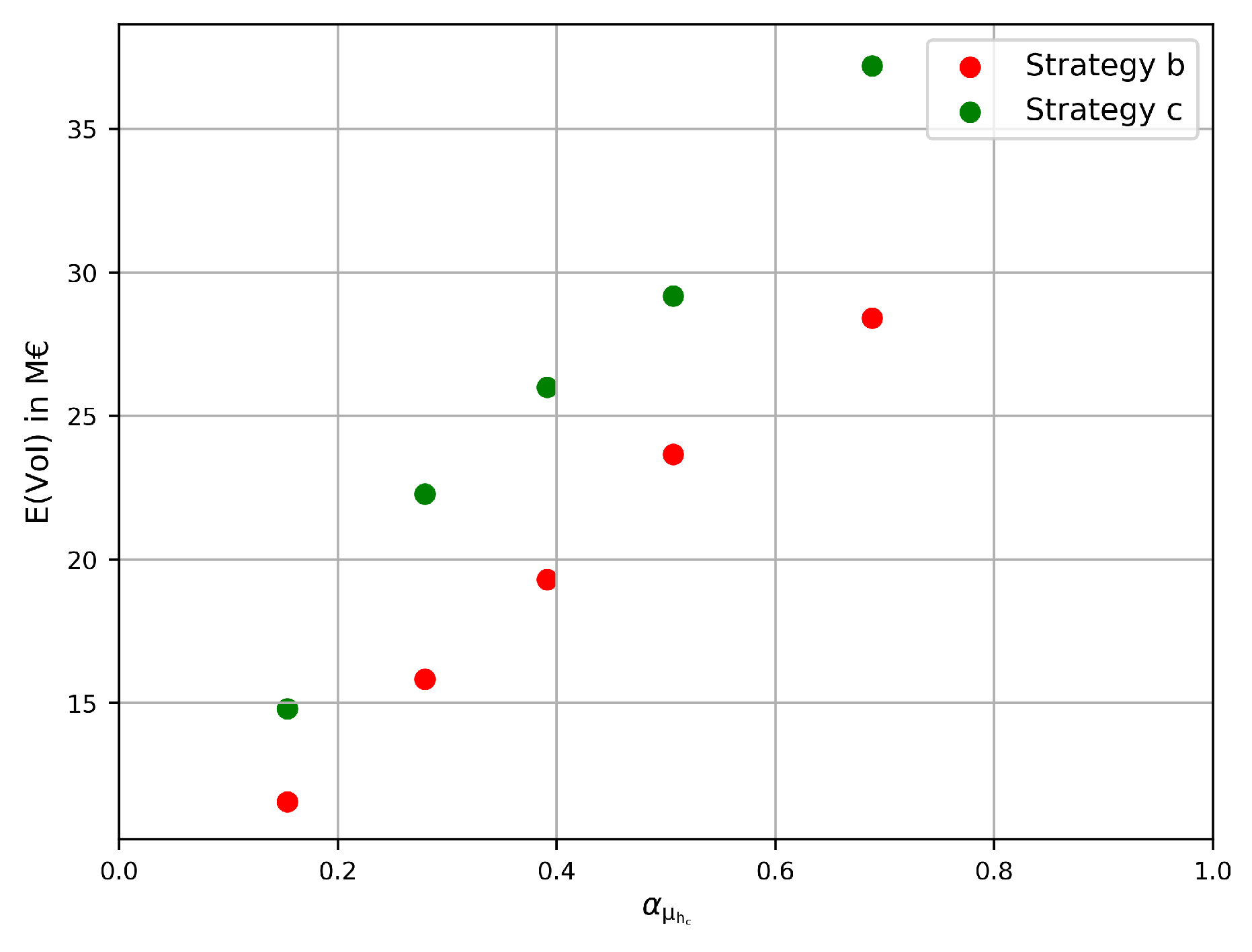
From the results with deterministic temporal changes, we see that there is a strong relation between the influence coefficient of reducible uncertainty in critical height ${\alpha }_{{\mu }_{\mathrm{h}}\mathrm{c}}$ and the VoI that is obtained (Figure 4), which is in line with the original hypothesis. In addition, the $P_{\mathrm{thresh}}$ at which valuable observations are obtained has a significant influence on VoI outcomes (Figure 6). Design loads for flood defences typically have very small probabilities of exceedance, meaning that deriving meaningful information from observed loads often requires that monitoring equipment is present during a relatively rare event. Hence, the fact that the VoI increases with observations of more extreme events has to be included in a decision analysis for a monitoring campaign. This can then be used to derive which duration of a monitoring campaign yields the highest Value of Information.

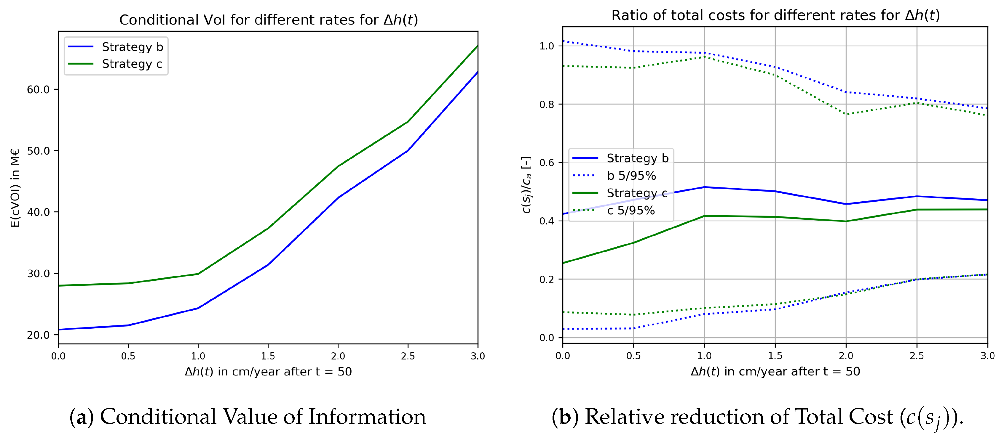
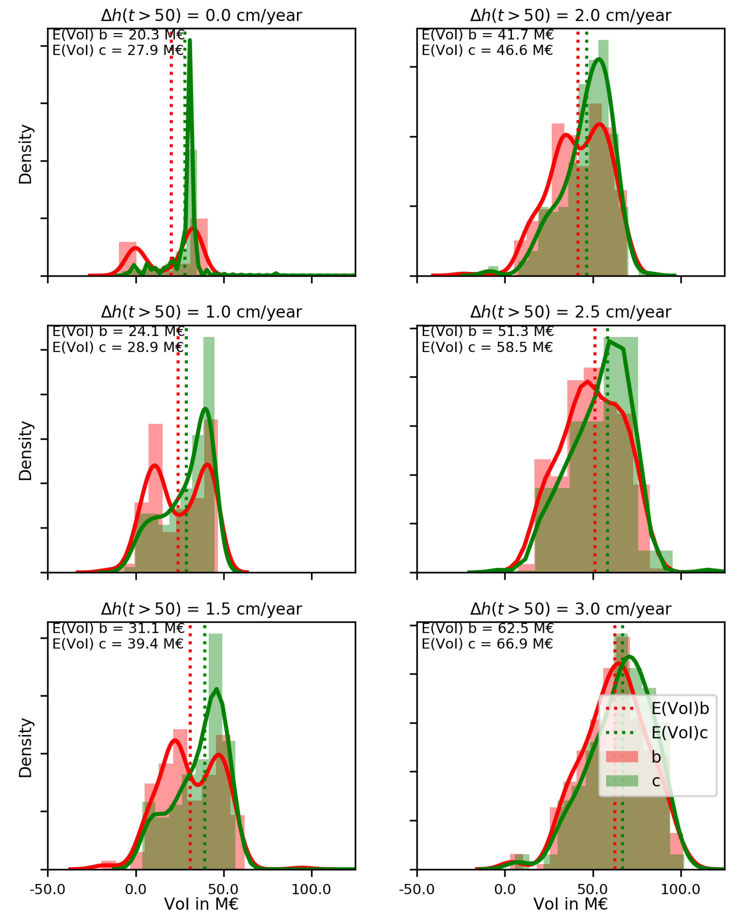
The final analysis presented deals with the effect of large uncertainty in future load conditions. In such cases, the investment required to deal with this uncertainty in design can be large. Hence, it is of interest to identify investment options that are beneficial in a wide variety of scenarios. In the analysis, it was shown that the conditional VoI can be a useful measure for this. A particular advantage is that it gives more insightful information than an expected VoI, which is of specific interest if there are other large uncertainties aside from the epistemic uncertainty that is reduced. It was shown that both the considered monitoring strategies have a positive VoI and yield a significant reduction of Total Cost in all considered future scenarios. Thus, investments in reducing epistemic uncertainties are concrete and economically efficient options for preparing for potentially large future changes in load conditions.

7. Conclusions

This paper has explored the benefits of Structural Health Monitoring for flood defences for long-term investments, specifically types of monitoring where the amount of information obtained depends on observed loads. A Bayesian pre-posterior decision model and the concept of Value of Information have been used to quantify the benefits of different monitoring strategies. It has been shown that the Value of Information is directly related to the relative influence of epistemic uncertainties, which can be easily obtained from probabilistic computations. In many cases, a monitoring campaign of some duration will be needed to reduce epistemic uncertainty. This has been investigated by comparing different threshold values at which information is obtained. The value of this threshold was found to have a major influence on monitoring outcomes and this aspect should therefore be considered in determining the duration of monitoring campaigns.

Many investments in flood defences have to consider large uncertainties in future loads due to climate change uncertainty. Therefore, the Value of Information of different scenarios for future load increase on a flood defence has also been considered. The Value of Information conditional on different rates of increase was found to be positive for all investigated rates. As Total Costs increase for higher rates of change, the relative cost reduction was similar over all different rates. Thus, Structural Health Monitoring aimed at reducing epistemic uncertainty is an economically efficient investment in preparation of potentially large future changes.