Effect of Scour on the Natural Frequency Responses of Bridge Piers: Development of a Scour Depth Sensor

Abstract

Local scour is the removal of soil around bridge foundations under the erosive action of flowing water. This hydraulic risk has raised awareness of the need for developing continuous monitoring techniques to estimate scour depth around bridge piers and abutments. One of the emerging techniques is based on monitoring the vibration frequency of either bridge piers or a driven sensor in the riverbed. The sensor proposed in this study falls into the second category. Some unresolved issues are investigated: the effect of the geometry and material of the sensor, the effect of the embedded length and the effect of soil type. To this end, extensive laboratory tests are performed using rods of different materials, with various geometries and lengths. These tests are conducted in both dry sand and a soft clayey soil. Since the sensor will be placed in the riverbed, it is crucial to evaluate the effect of immersed conditions on its response. A numerical 3D finite-element model was developed and compared against experimental data. This model was then used to compute the ‘wet’ frequencies of the sensor. Finally, based on both the experimental and numerical results, an equivalent cantilever model is proposed to correlate the variation of the frequency of the sensor to the scour depth.

1. Introduction

Scour is considered as the main cause of bridge damages [1] and accounts for nearly half of all bridge collapses in the USA [2]. In France, the collapses of the Wilson Bridge in Tours (1978) and the St Louis Bridge on Reunion Island (2007) serve as national examples of damages caused by scour [3]. In order to anticipate this risk, it is important to measure the current scour depth at bridge supports, namely the piers and abutments. On one hand, many empirical formulas are proposed in the literature [4,5,6,7]. However, most of them usually lead to an overestimation of its value [5] due to different factors including: scale effect since most of the equations are derived from flume test results, the simplifying hypothesis assumed for both bed material and flow and the difficulty of accurately measuring field data [8]. One the other hand, several monitoring devices already exist and are used in the field such as: float-out devices [9], radar [10,11], sonar [12], time domain reflectometry [13,14], magnetic sliding collar [15,16], electrical conductivity devices [17] and fiber optic [18,19]. However, those methods have several limitations such as: high sensitivity to noise, difficulties in result interpretations and not being suitable to high sediment concentration conditions. Therefore, recent studies attempt to suggest more accurate and practical monitoring techniques to evaluate scour at bridge foundations. An emergent technique based on the dynamic response of the structure is the main method proposed in this paper.

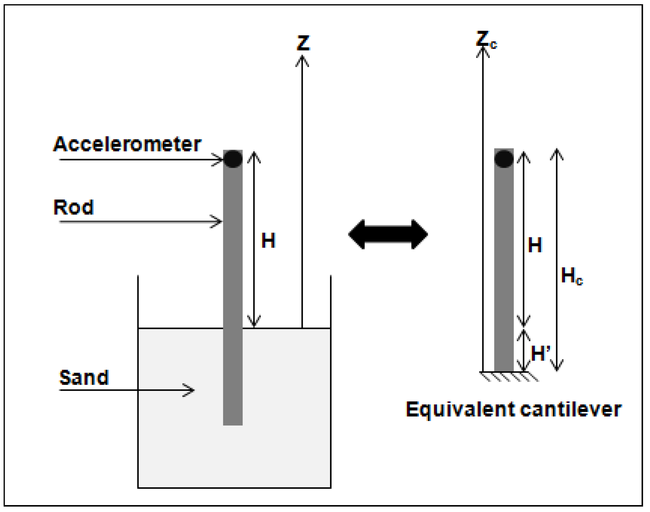
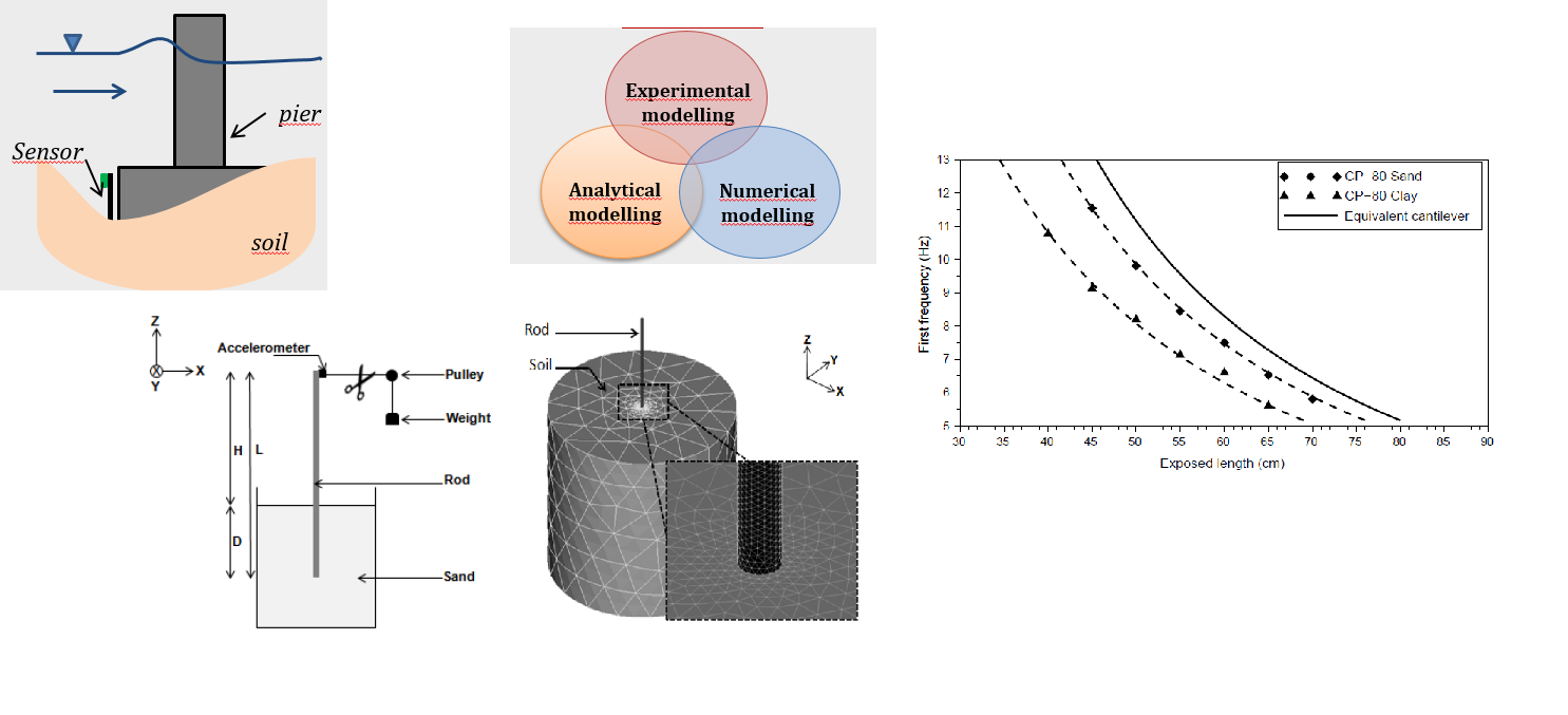
The principal of this monitoring technique is that scour causes an increase of the exposed length of the scoured structure. Consequently, based on the inverse relation between the fundamental frequency and the length of a cantilever beam, a decrease of the frequency can be correlated to an increase of scour depth [19,20]. Based on this result, two applications are generally proposed.

Zarafshan et al. [19] proposed to monitor bridge scour by means of rods embedded in the riverbed. Each rod is equipped with a fiber-optic Bragg grating sensor that uses the strain response history in the time domain to identify the fundamental frequency. In order to correlate the first frequency of the sensor to scour depth, a numerical model was developed based on the Winkler model of the soil. Once the rod is placed in the soil, its frequency is used to calculate the stiffness of the springs k used in the model. Then the model can be used to measure the first frequency for different scour depths.

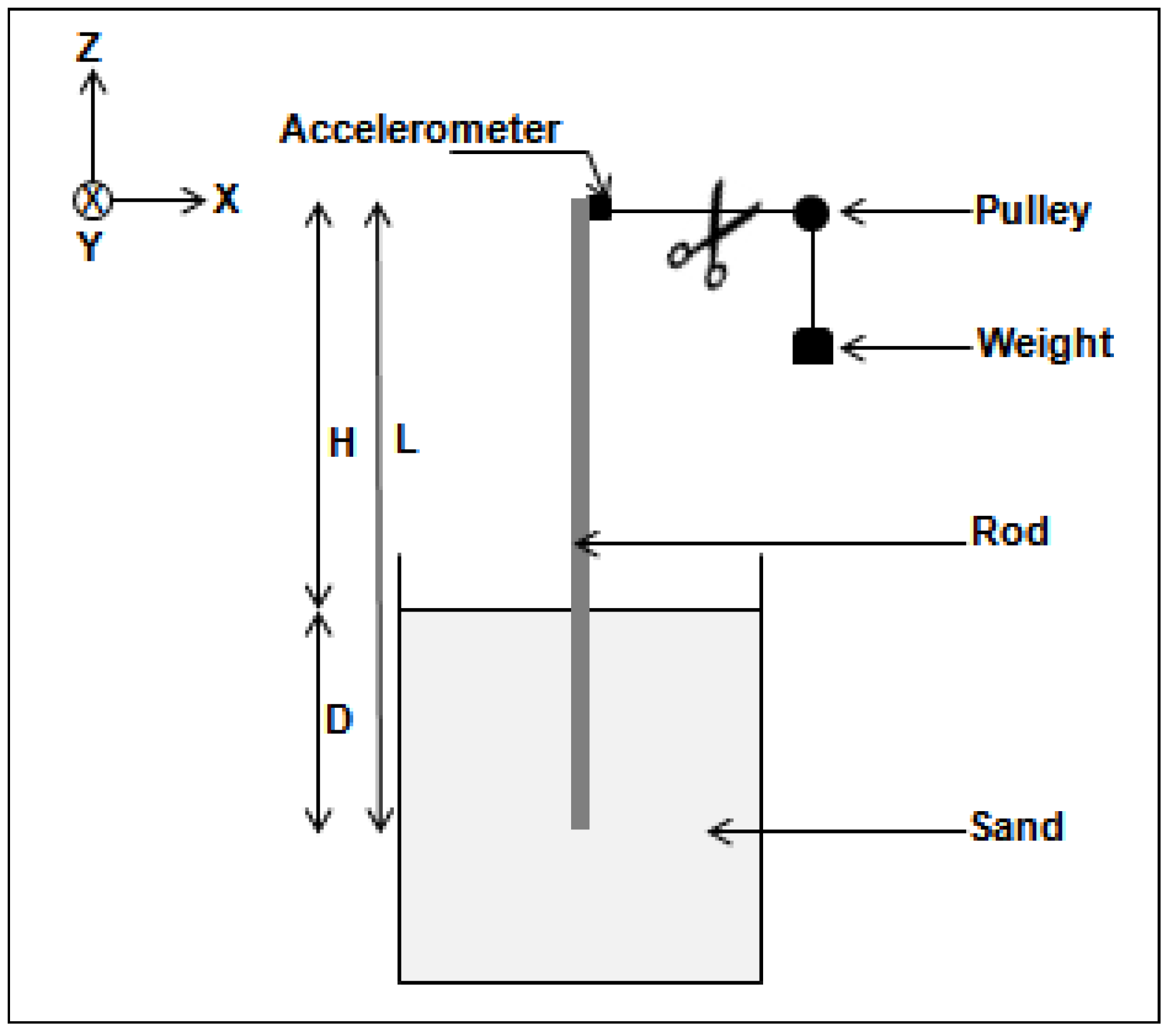
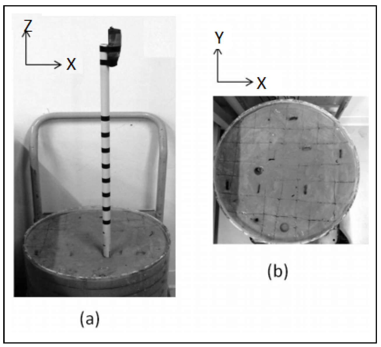
Prendergast et al. [20] proposed a direct approach, the effect of scour on the first frequency of the pile itself was studied. The experimental laboratory set-up consisted on a pile placed in a block of sand. Scour was simulated with the progressive extraction of a layer of the soil. For every scour depth, an impact was applied and the dynamic response of the pile recorded with an accelerometer placed on the top. The test showed that the first natural frequency decreases with the increase of the depth of the scour hole. The same experimental protocol was applied in situ to a 8.76 m in length pile and showed the same results. To establish a relation between the first frequency and the scour depth, a spring-beam finite element model was developed and validated. Unlike Zarafshan et al. [19] who used the vibration response of the sensor to determine the stiffness of the springs k, Prendergast et al. [20] used two geotechnical methods: the first one uses the small strain shear modulus $G_o$ determined with in-situ test with Multi-channel analysis of surface waves (MASW) or Cone Penetration Test (CPT) [21] and the second one uses the American Petroleum Institute design code (API).

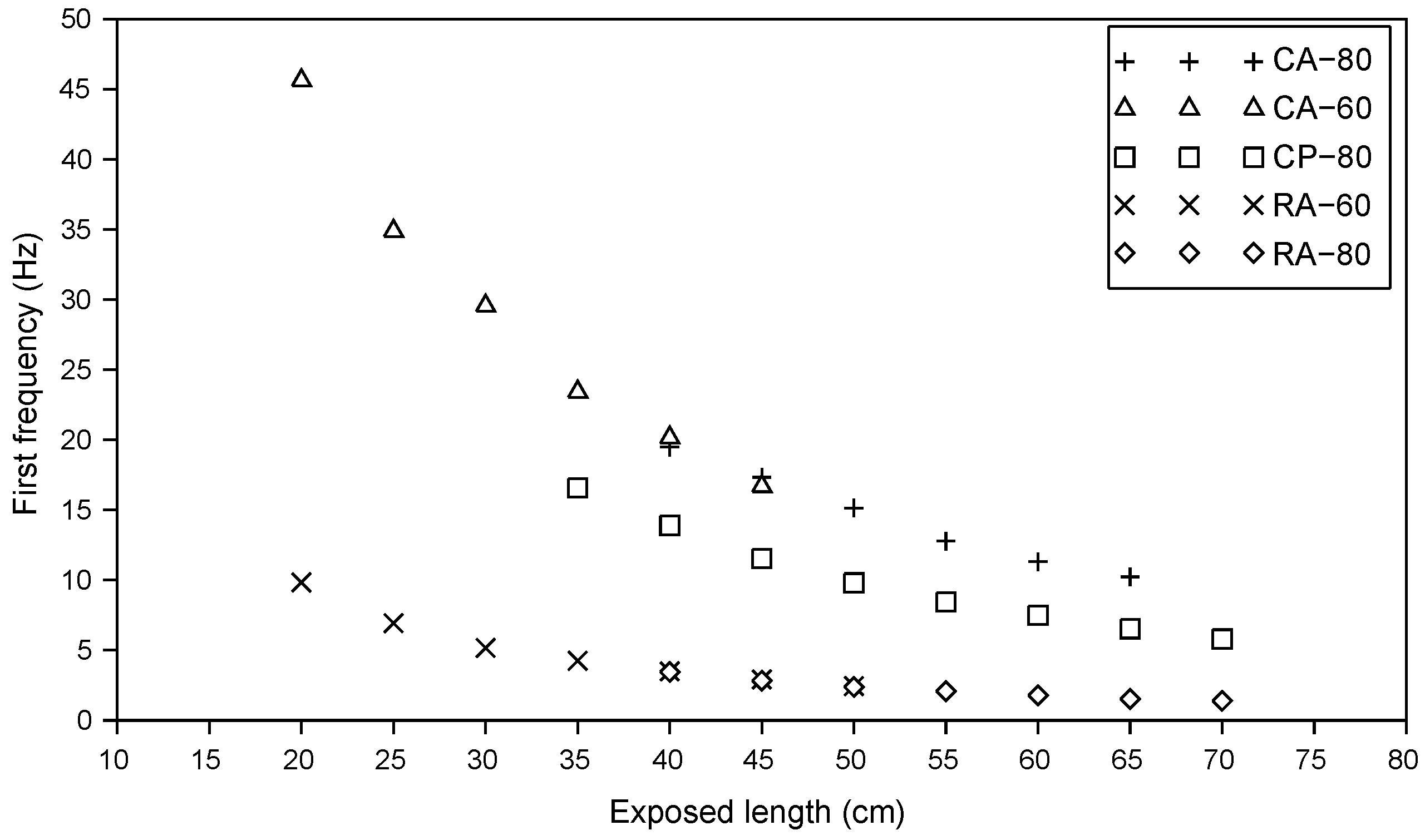
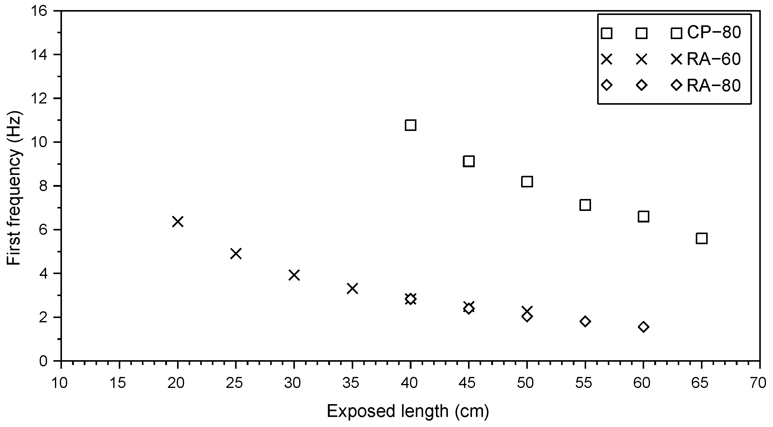
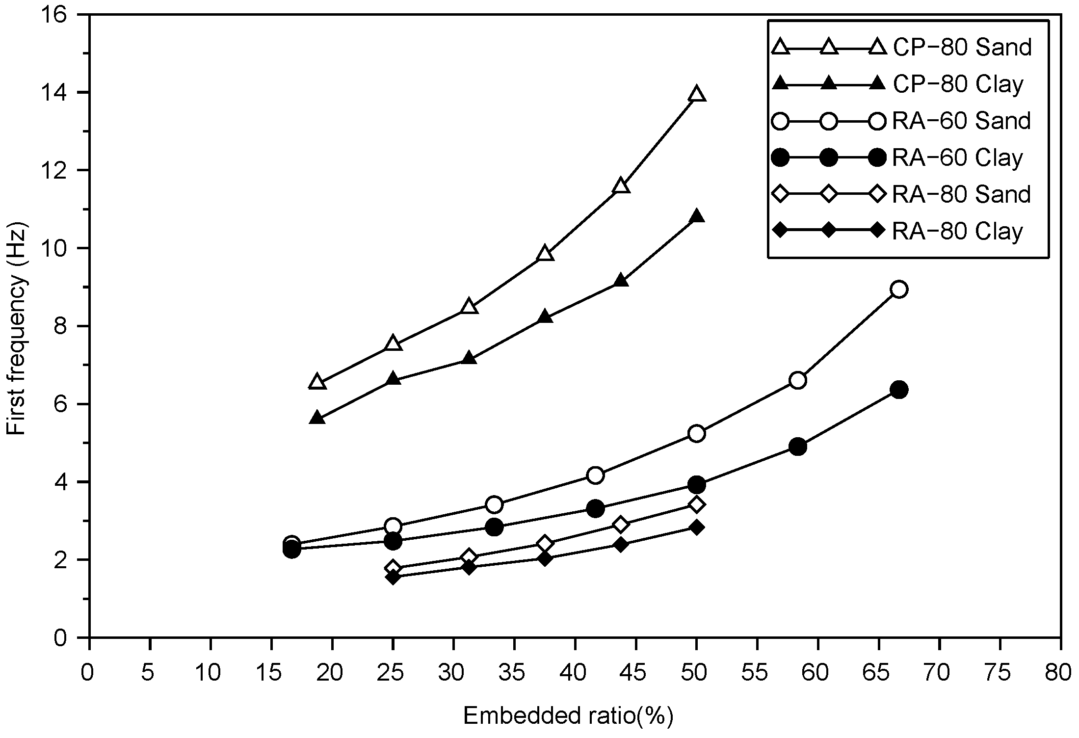
Both studies show that the first frequency of piles or sensors decreases with the increase of scour depth. However, the correlation between frequency and scour depth is not direct and requires the use of both a numerical model and experimental data to calibrate the spring stiffness. The present study focuses on the effect of scour on the dynamic response of sensor-rods partially embedded in soil, specifically on the correlation between the variation of the first frequency and the current scour depth. Some unsolved issues are also addressed such as: the effect of the sensor geometry and material, the effect of soil type and the effect of the embedded length.

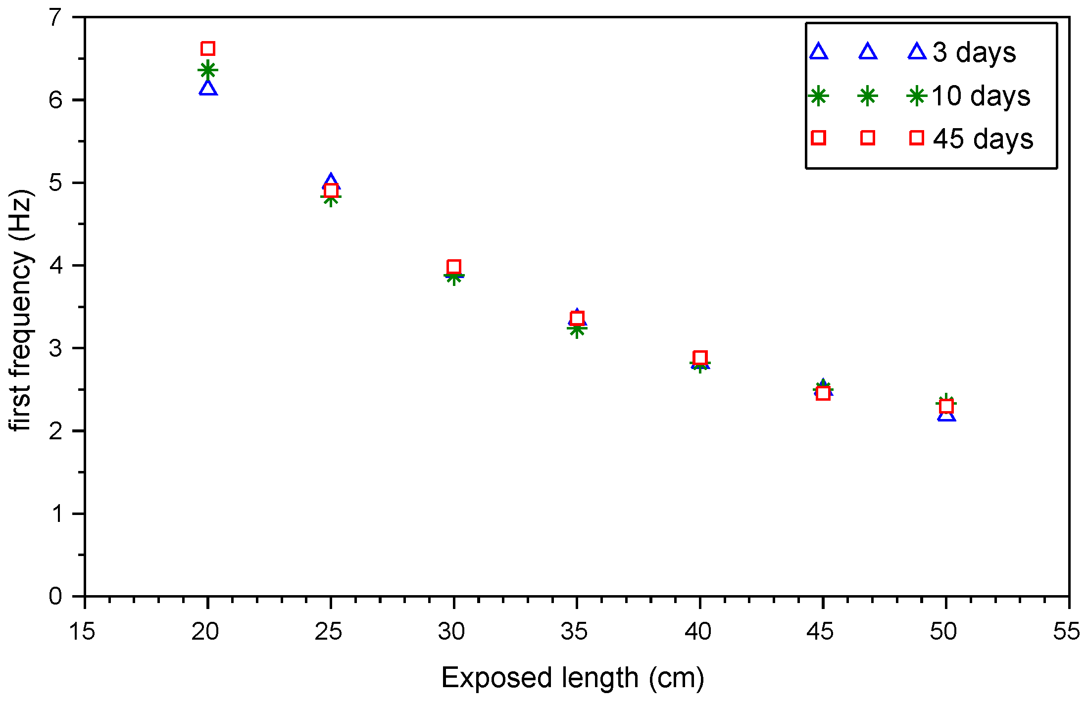
The paper starts in Section 2 with the description of the laboratory tests performed to assess the effect of scour on the first frequency of different rods in two type of soils. The repeatability of the measurement is evaluated and three important aspects are investigated: the sensitivity to the sensor material and geometry, the sensitivity to the embedded length and the effect of the soil. Then, in Section 3, a 3D numerical model is developed and validated. This model is then used to assess the effect of immersed conditions on the response of the sensor. 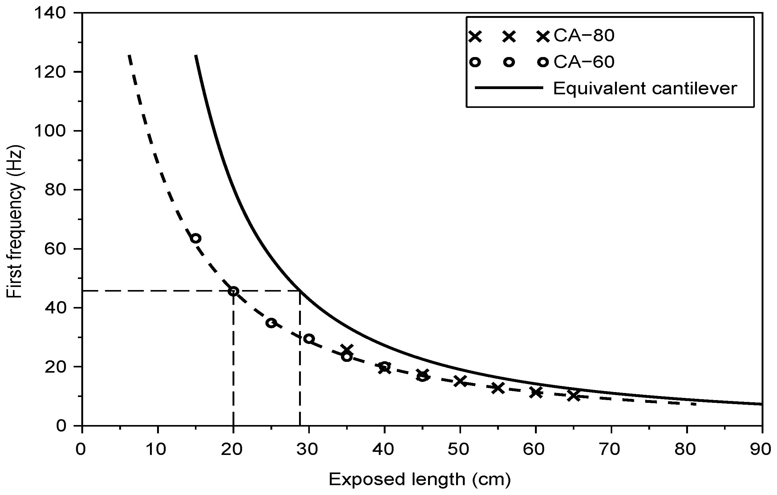In Section 4, the main results of this study are outlined and a simple method is proposed to correlate scour depth to the first frequency of an equivalent cantilever. Finally, in Section 5, conclusions and future use of the findings of this study are outlined.

2. Experimental Program

The experimental study conducted in the laboratory aims to investigate the feasibility of monitoring scour with rod-sensors. To this end, extensive tests are performed and the following issues are addressed: the effect of scour, the repeatability of the measurement, the effect of the sensor geometry and material, the effect of the embedded length and the effect of soil type.

2.1. Materials and Cross-Sections of the Rod-Sensor

In order to assess the effect of scour on the first frequency of the sensor, extensive laboratory tests are performed. Five rods having various geometries, lengths and material properties are tested: two circular aluminium rods of 800 mm and 600 mm length named CA-80 and CA-60 respectively, two rectangular aluminium rods of 800 mm and 600 mm length named RA-80 and RA-60 respectively and a circular PVC rod of 800 mm named CP-80. The geometrical and mechanical properties of each rod are summarized in Table 1. The tests are conducted in two type of soils: dry sand and a soft clayey soil. The experimental process in each soil is detailed in Section 2.2.

Table 1. Geometric and mechanical characteristics of the tested rods.

Tested Rods	Outer Diameter/Width (mm)	Thickness (mm)	Young Modulus (GPa)	Bulk Density (kg/m${}^3$)	Flexural Rigidity (N.m${}^2$)
CA-80, CA-60	12	1	59	2700	31.1
RA-80, RA-60	19	2	59	2700	0.8
CP-80	20	2	3.5	1425	11.0

2.2. Experimental Procedures

2.2.1. Sandy Soil

The experimental set-up is presented in Figure 1. A tank of 1 m × 1 m × 1 m in width, depth and height respectively is progressively filled with dry sand of Seine until it reaches a height of 0.7 m. Since the Young modulus of the soil $E_s$ is one of the most influencing parameters on the natural frequency of the soil-rod system [22], its value is measured and is used afterward in the numerical model. For this purpose, a mini-pressuremeter test [23] is conducted to determine the average value of the Ménard modulus $E_m$. The Young modulus $E_s$ is then calculated using Equation (1) [24]:

$$E_s=\frac{E_m}{\alpha },$$

(1)

where $\alpha$ a rheological parameter ($\alpha$ = 1/3 for sand). The properties of the dry sand used in this study are summarized in Table 2.

Figure 1. Laboratory set-up in dry sand, where the tank at the bottom has a volume of 1 m × 1 m × 1 m and can be filled up to 0.7 m by sand.

Table 2. Dry sand properties.

${\mathit{D}}_{50}$ (mm)	${\mathit{\rho }}_{\mathit{s}}$ (Kg/m${}^3$)	${\mathit{\nu }}_{\mathit{s}}$	${\mathit{E}}_{\mathit{m}}$ (MPa)	${\mathit{E}}_{\mathit{s}}$ (MPa)
0.7	1700	0.3	0.5	1.5

The sensor is then placed in the soil volume. A thread connects the top of the rod, through a pulley, to a known dead weight. To generate an impulse force of a known amplitude, ensuring similar testing conditions, the thread is cut inducing the vibration of the sensor in the X direction. An accelerometer having a mass of m = 41 g, is placed on the top of the rod since it has been proved to be the optimal location [25]. The accelerometer records the transient dynamic response of the sensor corresponding to its first bending mode of vibration.

The scour process is taken into account by the progressive increase of the exposed length H of the sensor. Table 3 summarizes the range of the exposed length H for each rod. This length is limited on the one hand by the tank dimensions, and on the other hand by the stability of the rod-sensor. The scour depth is increased step by step with increments of 50 mm. For each exposed length H, the impulse force is applied and the vibratory response of the rod is recorded. The data samples are recorded with a sampling frequency of 512 Hz. The transient response of the system is then post processed using SCILAB to measure the first natural frequency from the Fast Fourier Transform (FFT). To evaluate the accuracy of the measurement, each test is repeated three times.

Table 3. Range of exposed length H of the rods in dry sand.

Tested Rods	Min H (cm)	Max H (cm)
CA-80	35.0	65.0
CA-60	15.0	45.0
RA-80	35.0	70.0
RA-60	15.0	50.0
CP-80	35.0	70.0

2.2.2. Clayey Soil

A soft saturated clayey soil mixture is prepared with of 50% sand of Fontainebleau, 50% of Armoricaine Kaolinite clay and 25% water [26,27]. A Plexiglas cylinder of 400 mm diameter and 400 mm height is progressively filled with the mixture. To ensure a uniform density, the soil specimen is manually compacted into five layers of equal thickness. The soil mixture is matured during 48 h. The experimental protocol used in sand is adapted to the clayey soil. Due to the high plasticity of the soil mixture (Figure 2), an impact is applied to generate the impulse in order to avoid the deformation of the soil induced by the previous protocol before the beginning of the testing.

Figure 2. Photographs of (a) laboratory setup in clayey soil; (b) plastic deformation of the soil.

The aging of clayey soils often improves their mechanical properties [28] which can induce a variation of the rods frequencies. To make sure that the changes of the frequency are caused only by scour, vibration tests of the rod RA-60 are conducted after three days, ten days and forty-five days. Table 4 summarizes the range of the exposed length H for each rod in the clayey soil.

Table 4. Range of exposed length H of the rods in clayey soil.

Tested Rods	Min H (cm)	Max H (cm)
RA-80	40.0	60.0
RA-60	20.0	50.0
CP-80	40.0	65.0

It should be noted that tests of the circular aluminum rods CA-80 and CA-60 showed no vibratory response due to their high flexural rigidity (see Table 1). In fact, if the structure is more rigid than the soil, the response of the structure is restricted to rigid body modes [29]. Consequently, no results are available for the rods CA-80 and CA-60 in the clayey soil.

3. Numerical Model

A numerical model is created to validate and understand the experimental results.

Moreover, in practice, the sensor will be placed in the riverbed and immersed in water. Therefore, it is crucial to asses the effect of water on the response of the sensor. To this end, a finite element model is developed.

3.1. Theoretical Formulation

The evolution of multiple-degree-of-freedom system is expressed by the following equation:

$$\left[\mathbf{M}\right]\left\{\ddot{\mathbf{u}}\right\}+\left[\mathbf{C}\right]\left\{\dot{\mathbf{u}}\right\}+\left[\mathbf{K}\right]\left\{\mathbf{u}\right\}=\left\{\mathbf{F}\right\}$$

(2)

where $\left[\mathbf{M}\right]$, $\left[\mathbf{C}\right]$ and $\left[\mathbf{K}\right]$ are respectively the mass, the damping and the stiffness matrices; $\left\{\ddot{\mathbf{u}}\right\}$, $\left\{\dot{\mathbf{u}}\right\}$ and $\left\{\mathbf{u}\right\}$ are respectively the acceleration, the velocity and the displacement and $\left\{F\right\}$ the external vector force applied to the system. The dimension of the matrices is $N\times N$, where N is the number of degrees of freedom of the system.

In the absence of damping, the free vibrations of the structure are described with the eigenvalue problem:

$$\left[\mathbf{M}\right]\left\{\ddot{\mathbf{u}}\right\}+\left[\mathbf{K}\right]\left\{\mathbf{u}\right\}=0$$

(3)

The solution of Equation (3) can be written $\left\{\mathbf{u}\right\}=\left\{\mathbf{U}\right\}{exp}^{i\omega t}$, which leads to :

$$(-\left[\mathbf{M}\right]{\omega }^2+\left[\mathbf{K}\right])\left\{\mathbf{U}\right\}=(-\left[\mathbf{M}\right]\lambda +\left[\mathbf{K}\right])\left\{\mathbf{U}\right\}=0$$

(4)

with $\lambda ={\omega }^2={\left(2\pi f\right)}^2$, f the natural frequency and $\left\{\mathbf{U}\right\}$ the mode shape. This linear system has N non trivial solutions ($U_i$, ${\lambda }_i$) [$i=1,2,3,\dots ,N$] [30] that verify the theoretical condition:

$$det(\left[\mathbf{K}\right]-{\lambda }_i\left[\mathbf{M}\right])=0$$

(5)

Since only the first frequency is needed, a subspace iteration method [31] is used to solve the system.

3.2. Model Description

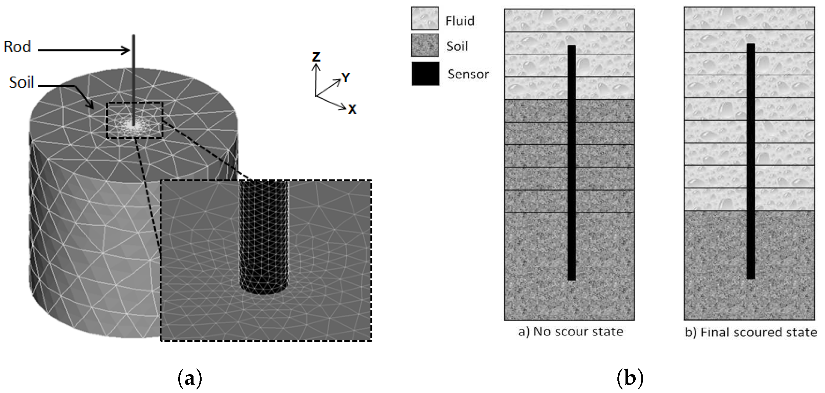
A 3D finite elements model is developed using the finite element software Code-Aster [32]. The proposed model is based on the following hypothesis: (1) the soil medium and the rod-sensor are elastic, (2) all displacements and strains remains small and (3) the soil and the sensor are perfectly bounded at the interface. For the boundary conditions, the lateral faces of the soil are fixed against displacement in the normal direction and the base is fixed against displacement in all directions. The weight of the accelerometer is not negligible and is modeled as a nodal mass placed at the top of the rod-sensor. In this model, the soil and the sensor are meshed with 10 nodes tetrahedron elements. The mesh was refined near the sensor with a progressive transition to a coarser mesh away from the sensor. The average number of mesh nodes was fixed to 80,000 after conducting a mesh convergence analysis for each tested rod. Figure 3a shows the three-dimensional numerical model of the rod-soil system.

Figure 3. Finite elements scour model. (a) Three-dimensional numerical model of the rod-soil system and mesh details; (b) Scour simulation with the numerical model.

In order to simulate scour process in immersed conditions, the numerical model is partitioned to several layers of 50 mm thickness. The initial scour state is presented in Figure 3b. As scour increases, the soil layers are progressively replaced by fluid layers, mimicking the natural phenomenon. This substitution is achieved by modifying the material properties of the given layer. This approach is therefore only valid if water does not change the general behavior of the rod compared to the case without water [33].

The material properties used in the model are those of dry sand and the rods presented in Table 1 and Table 2. No readjustments of the parameters is performed afterwards.

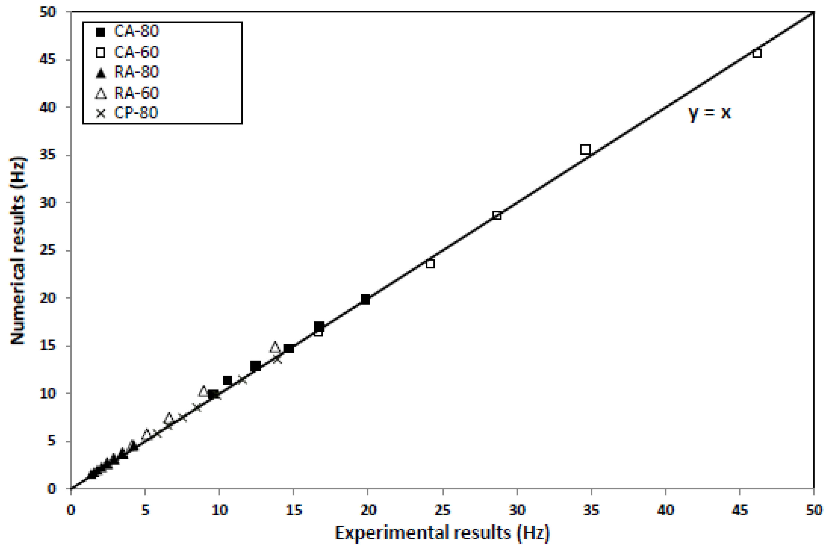
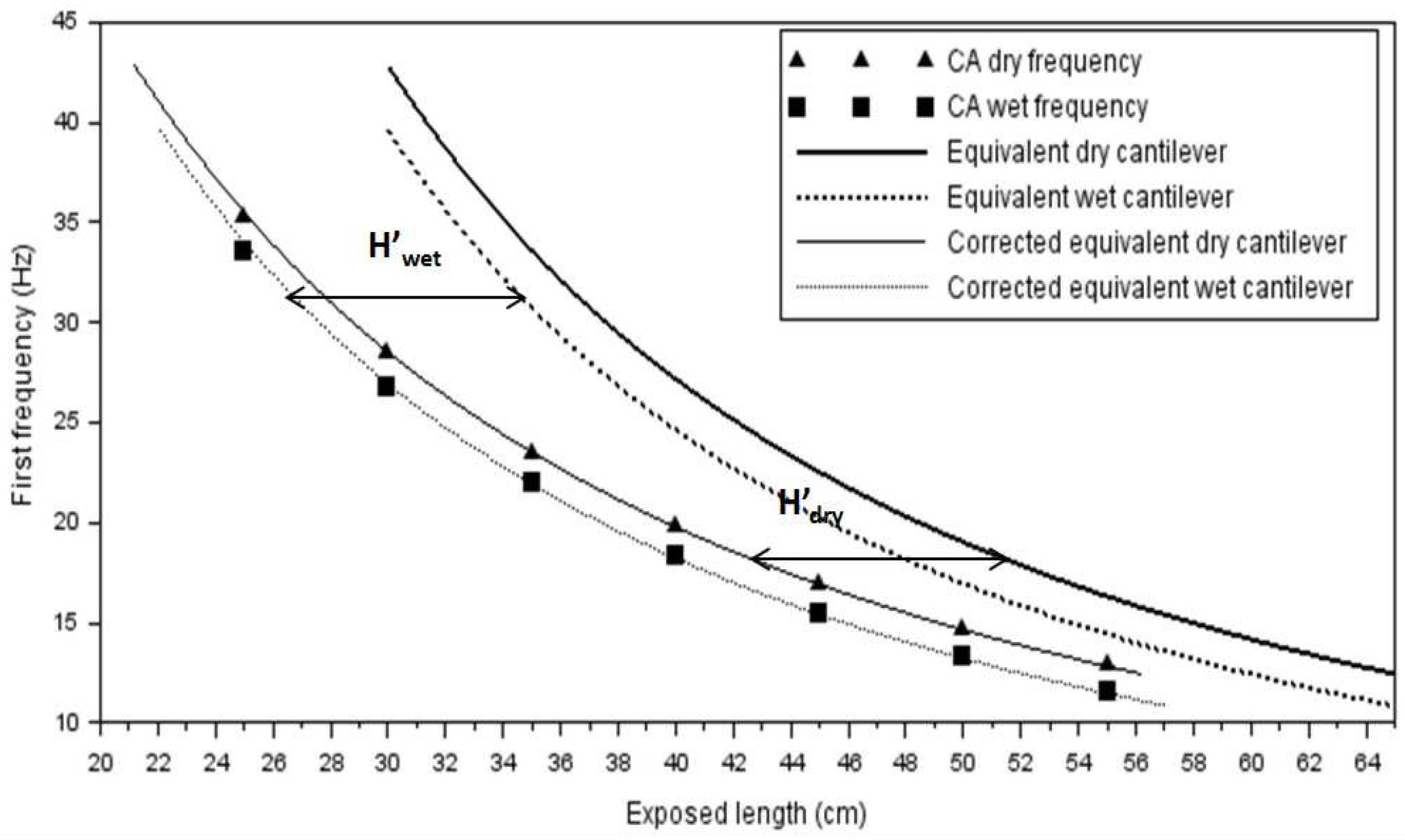
First, the model is used to compute the dry frequencies of all tested rods (without the fluid). The first numerical frequency corresponding to the bending mode of the rods is compared to experimental data to validate the model for each exposed length.

Then, in order to assess the effect of the immersed condition on the sensor response, the wet frequencies (with the fluid) of the circular aluminum rods (CA-60 and CA-80) are computed following the procedure described previously as shown in Figure 3.

4. Results and Discussion

4.1. Experimental Results

4.1.1. Effect of Soil Aging

The results of the vibration tests of the rod RA-60 at different dates are presented in Figure 4. There is no clear tendency of the evolution of the frequency with the aging of the clayey soil mixture. Consequently, the variation of the frequency, during the testing period, is not a result of the improvement of the mechanical characteristics of the soil.

Figure 4. Variation of first frequency with exposed length H in the clayey soil after 3, 10 and 45 resting days.

4.1.2. Repeatability Analysis

The accuracy of the sensor is evaluated in dry sand for the rods CA-80, RA-80 and CP-80. The three measured frequencies for the minimum exposed length H = 35 cm and the maximum exposed length H = 65 cm are summarized in Table 5. The results indicates that the standard deviation, for the three tested rods, at each exposed length is less than 0.50 Hz. This demonstrates the accuracy of the sensor measurement.

Table 5. Repeatability analysis in dry sand.

Exposed Length	CA-80		RA-80		CP-80
	Measured Freq. (Hz)	Average Freq. (Hz)	Measured Freq. (Hz)	Average Freq. (Hz)	Measured Freq. (Hz)	Average Freq. (Hz)
	9.52		1.55		6.58
H = 65 cm	9.98	9.64 ± 0.30	1.56	1.55 ± 0.01	6.50	6.51 ± 0.07
	9.42		1.55		6.45
	25.33		4.21		16.94
H = 35 cm	26.28	25.71 ± 0.50	4.11	4.14 ± 0.06	16.18	16.58 ± 0.38
	25.53		4.10		16.61

4.1.3. Effect of Scour

Figure 5 displays the experimental results in dry sand. The first frequency of the sensors decreases with the increase of the exposed length H. This trend is in full agreement with the results of [19,20]. As shown in Figure 6, a similar tendency in noticed in the clayey soil.

Figure 5. Variation of first frequency with exposed length in sandy soil.

Figure 6. Variation of first frequency with exposed length in clayey soil.

Table 6 shows the frequency of the rods in both soils for the exposed lengths H = 60 cm and H = 40 cm, representing 20 cm scour. To compare the sensitivity of the tested rods to scour, a frequency change rate p is defined with Equation (6):

$$p=\frac{f_{(H=40)}-f_{(H=60)}}{f_{(H=40)}}$$

(6)

Table 6. Sensitivity of the frequencies of the tested rods to scour in sand and clayey soil.

Tested Rods	Flexural Rigidity N.m${}^2$	Frequencies in Sand			Frequencies in Clayey Soil
		H = 60 cm	H = 40 cm	Change Rate $\mathit{p}$ (%)	H = 60 cm	H = 40 cm	Change Rate $\mathit{p}$ (%)
CA-80	31.1	11.31	19.50	42	-	-	-
CP-80	11.0	7.50	13.90	46	6.6	10.78	39
RA-80	0.8	1.78	3.45	48	1.53	2.8	45

It can be seen that the frequency change rate p increases with the flexural rigidity of the tested rod in both sand and clayey soil. The sensitivity of the rods is also affected by the soil. For instance, the frequency of the rod CA-80 varies by 46% is sand and 39% in soft clayey soil for the same scour depth.

4.1.4. Effect of the Embedded Length

The effect of the embedded length D is investigated. Figure 5 and Figure 6 show that the rods CA-80 and CA-60 have the same frequency when their exposed length H is equal, even if their embedded length D are different. Similar results are observed for the rods RA-80 and RA-60 in both soil types. This means that the frequency is more influenced by the exposed length H rather than the embedded length D in our experimental conditions.

4.1.5. The Effect of Soil Type

In order to highlight the effect of the soil type on the frequency of the sensor, the variation of the first frequency with the embedded ratio of the rods RA-80, RA-60 and CP-80 is shown in Figure 7 for sand and clayey soil.

Figure 7. Variation of first frequency with embedded ratio in sand and clayey soil.

The results show that the frequencies in sand are higher than the frequencies in the clayey soil. This is mainly due to the higher stiffness of sand compared to the lower stiffness of the clayey soil with high plasticity used in this study. For low embedded ratios, the first frequency of the rods in both soils is almost similar. But as the embedded ratio increases, the gap between the frequency curves in sand and in clayey soil increases. This implies that for high embedded ratio, the frequency of the rod is significantly influenced by the stiffness of the soil it is embedded in.

4.2. Numerical Results

4.2.1. Model Validation

The numerical frequencies of all tested rods are compared to the experimental frequencies in dry sand. Figure 8 shows that the numerical and experimental results are in good agreement without any readjustment of parameters.

Figure 8. Comparison of experimental and numerical first frequencies of the tested rods (correlation coefficient of $R^2=0.9905$).

4.2.2. The Effect of Water

The effect of water on the frequency of the sensor is investigated. Following the numerical procedure described is Section 3.2, the wet frequencies of the rods are calculated for each exposed length H. As shown in Table 7, water decreases the frequency of the sensor. As scour increases, the effect of water becomes more significant with changes from 4% for H = 25 cm to 9% for H = 55 cm.

Table 7. Comparison between wet and dry frequencies of the circular aluminum (CA) rods.

Exposed Length	Dry Frequency	Wet Frequency	Percentage Change of the Frequency
(cm)	(Hz)	(Hz)	Between Air and Water (%)
55	12.8	11.6	9
50	14.6	13.3	9
45	16.8	15.5	8
40	19.7	18.3	7
35	23.4	21.9	6
30	28.3	26.8	5
25	35.2	33.6	4

4.3. Proposed Calibration Technique of the Sensor

4.3.1. Equivalent Cantilever Beam

The variation of the experimental first frequencies of the tested rods, in sand and clayey soil, is compared to the response of a cantilever beam with a punctual mass attached at its free end to take into account the accelerometer. The free length of the cantilever is called $H_c$, the total mass of the cantilever M and the mass of the accelerometer m. The theoretical frequencies of the cantilever are calculated using Equation (7) [34,35] and are plotted with a continuous line in Figure 9, Figure 10 and Figure 11.

$$f_{th}=\frac{1}{2\pi }\times \sqrt{\frac{3EI}{{H_c}^3(0.24M+m)}}$$

(7)

Figure 9. Equivalent cantilever of CA rod-sensors in sand: experimental first frequency for road-sensors CA-80 and CA-60, and first frequency of equivalent cantilever beam $f_{th}={\displaystyle \frac{1}{2\pi }}\times \sqrt{{\displaystyle \frac{3EI}{{H_c}^3(0.24M+m)}}}$.

Figure 10. Equivalent cantilever of rectangular aluminium (RA) rod-sensors in sand and clayey soil: experimental first frequency for road-sensor RA-80 and RA-60 in both sand and clayey soil, and first frequency of equivalent cantilever beam $f_{th}={\displaystyle \frac{1}{2\pi }}\times \sqrt{{\displaystyle \frac{3EI}{{H_c}^3(0.24M+m)}}}$.

Figure 11. Equivalent cantilever of circular PVC (CP) rod-sensor in sand and clayey soil: experimental first frequency for road-sensor CP-80 and RA-60 in both sand and clayey soil, and first frequency of cantilever beam $f_{th}={\displaystyle \frac{1}{2\pi }}\times \sqrt{{\displaystyle \frac{3EI}{{H_c}^3(0.24M+m)}}}$.

It appears that all tested rods and in both soil types, the theoretical results of the cantilever are horizontally translated against the experimental results with a constant $H^{\prime }$. This adjustment length $H^{\prime }$ varies with the sensor and the soil characteristics.

The physical meaning of $H^{\prime }$ is related to the soil-rod interaction which does not correspond to a perfect cantilever, but may match this assumption from a distance $H^{\prime }$ under the soil surface. Therefore, for each value of the exposed length H, the first natural frequency of the rods in each soil is equal to the frequency of an equivalent cantilever with a free length $H_c=H+H^{\prime }$ (Figure 12). For instance, to estimate the experimental first frequency of the circular rod in the sand with an exposed length $H=20$ cm, Equation (8) is used:

$$f_{exp}(H=20)=f_{the}(H_c=20+8.8=28.8)=45.7\mathrm{Hz}$$

(8)

Figure 12. Equivalent cantilever of the dynamic soil structure interaction.

The inverse relationship between the first frequency and the free length (9) derived from Equation (7) can be used to determine the scour depth $y_s$, see Equation (9):

$$H=\sqrt[3]{{\left(2\pi f_{exp}\right)}^2\times \frac{0.24M+m}{3EI}}-H^{\prime }\Rightarrow y_s=H-H_0$$

(9)

The values of this adjustment length for all tested rods and soils are summarized in Table 8.

Table 8. Value of the equivalent length of the tested rods in both soils.

Tested Rod	Corrected Length in Sand (cm)	Corrected Length in Clayey Soil (cm)
CA-80, CA-60	8.8	No results
RA-80, RA-60	4	11
CP-80	4.6	11

4.3.2. Wet Frequencies and Equivalent Cantilever Beam

In practice, the sensor will be placed in the riverbed and immersed in water. Therefore, it is crucial to verify the validity of the proposed calibration technique when the sensor in completely immersed. The calculated wet frequencies in Section 4.2.2 are first compared to the cantilever frequencies derived from Equation (7) but an adjustment length could not be derived. It seems more appropriate to compare the wet frequencies of the sensor to the wet frequencies of a cantilever derived from Equation (10):

$$f_{wet}=\frac{1}{2\pi }\times \sqrt{\frac{3EI}{{H_c}^3[0.24(M+M_a)+m]}},$$

(10)

where $M_a$ is the added mass of the fluid. Figure 13 shows that the wet frequencies of the sensor are indeed translated against the theoretical frequencies of the immersed cantilever. However, the value of the adjustment length in immersed conditions is $H_{wet}$ = 8 cm against $H_{dry}$ = 8.8 cm in dry condition.

Figure 13. Equivalent cantilever of the circular rod in dry and wet conditions.

4.4. Sensitivity Study

The experimental tests show that the adjustment length $H^{\prime }$ vary with the geometry of the sensor and the soil type. In order to identify the parameters influencing this length, the numerical model detailed in Figure 3b is used to perform a sensitivity study. The effect of three parameters is investigated: the Young modulus of the rod $E_r$, the bulk density of the rod ${\rho }_r$ and the Young modulus of the soil $E_s$. The results of the numerical simulation which are presented here, have been performed using the rod CA-80.

4.4.1. The Effect of the Elasticity of the Rod-Sensor $E_r$

The frequencies of the rod are calculated for three values of $E_r$: 100 GPa, 59 GPa and 5.9 GPa. The results are then compared to the frequencies derived from Equation (7) of an equivalent cantilever with a similar Young modulus. The value of the adjustment length $H^{\prime }$ can then be estimated. Figure 14 shows that the adjustment length $H^{\prime }$ increases with the increase of the Young modulus of the rod $E_r$.

Figure 14. Variation of the adjustment length $H^{\prime }$ with the Young modulus of the rod $E_r$.

Once again, the experimental frequencies and the first frequency of the equivalent beam are in good agreement.

4.4.2. The Effect of the Density of the Rod-Sensor ${\rho }_r$

The frequencies of the rod are calculated for three values of ${\rho }_r$: 1300 kg·m${}^{-3}$, 2700 kg·m${}^{-3}$ and 7500 kg·m${}^{-3}$. The results are then compared to the corresponding equivalent cantilever to estimate the value of the adjustment length $H^{\prime }$. Figure 15 shows that the adjustment length $H^{\prime }$ is independent of the bulk density of the rod ${\rho }_r$.

Figure 15. Variation of the adjustment length $H^{\prime }$ with the bulk density of the rod ${\rho }_r$.

4.4.3. The Effect of the Elasticity of the Soil $E_s$

The frequencies of the rod are calculated for three values of $E_s$: 1.5 MPa, 15 MPa and 150 MPa. The results are then compared to the equivalent cantilever to estimate the value of the adjustment length $H^{\prime }$. Figure 16 provides the value of $H^{\prime }$ for each value of $E_s$.

Figure 16. Variation of the adjustment length $H^{\prime }$ with the Young modulus of the soil $E_s$.

As it can be seen, $H^{\prime }$ decreases from 8.8 cm to 2.4 cm when the stiffness of the sol varies between 1.5 MPa and 150 MPa. This result was predictable since the equivalent cantilever is the specific case where the soil has an infinite stiffness. In that case, the rod is completely fixed at the ground surface and $H^{\prime }=0$. As the stiffness of the soil decreases, the rod should be embedded deeply to insure a similar constraint as the clamped condition.

The results of the sensitivity study have a practical interest. In fact, in the field, the only variable input is the sensor, which means its geometry and its material characteristics. It would be wise to try reducing the adjustment length $H^{\prime }$ of the sensor so that the cantilever model can be used to predict the frequencies of the sensor with reasonable accuracy. The results show that this can be achieved by varying the geometry and decreasing the Young modulus of the sensor.

4.5. General Discussion about the Findings

Zarafshan et al. [19] proposed the concept of fiber optic instrumented rods as scour-depth sensors. In that case, the scour depth is obtained by the deformation of the rod. Here, it has been shown that this approach is also valid for rods instrumented by accelerometres. The existence of scour is proven by changes in the first frequency of the rod itself, and the depth can be assessed through this innovative equivalent cantilever beam approach.

This brings about a low cost sensor, which may be complementary to direct bridge monitoring as proposed by Prendergast et al. [20].

5. Concluding Remarks and Perspectives

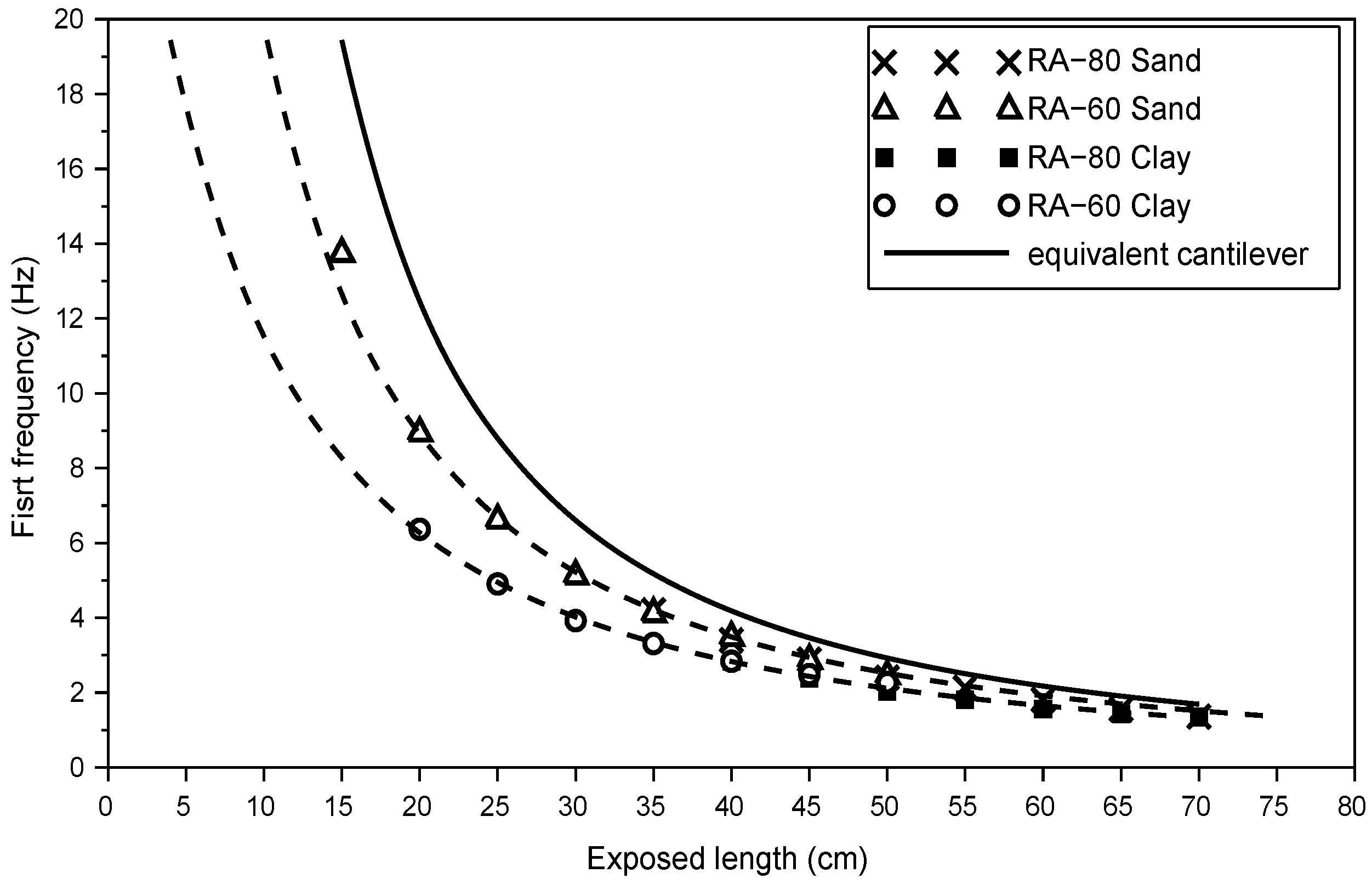
Scour is one of the major risks threatening the stability of bridges across rivers and in coastal areas. Therefore, it is paramount to evaluate the current scour depth around piers and abutments. The reported study proposes a continuous monitoring technique of scour by means of rods embedded in the riverbed. Extensive experimental tests were performed in the laboratory using various rods and two types of soil: dry sand and a soft clayey soil. Some uncovered issues were investigated: the effect of the geometry and material of the sensor, the effect of its embedded length and the effect of soil type. The results showed that the sensitivity of the sensors decreases with their flexural rigidity. Furthermore, when the flexural rigidity of the sensor is high in respect to the soil stiffness, no vibratory response was recorded since the response of the sensor was limited to rigid body motion. Thus, it is necessary to select the sensor material and geometry carefully depending on the stiffness of the soil it will be placed in. The tests also showed that the effect of soil type is less significant when the embedded ration of the rod decreases, in other words, when scour increases. Since the sensor will be immersed in water around the pier, the effect of water on the response of the sensor was investigated using a finite element model, and by assuming that the water does not change the behavior of the rod. The numerical results indicate that the effect of water should not be neglected. Indeed, as scour increases, the effect of water becomes more significant.

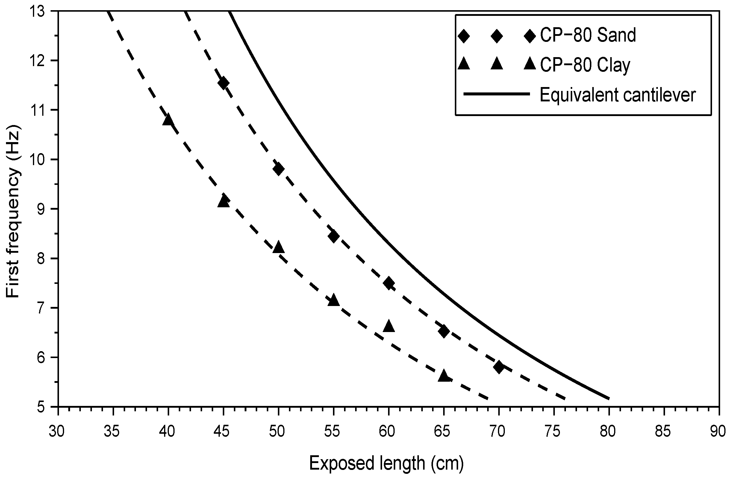
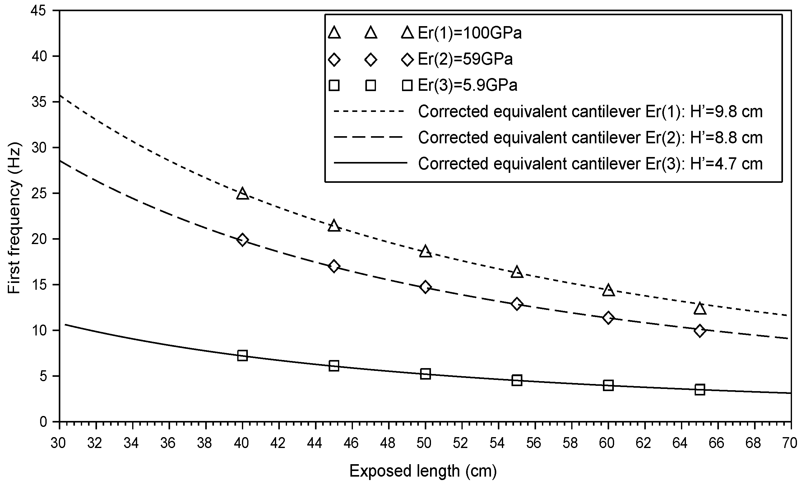
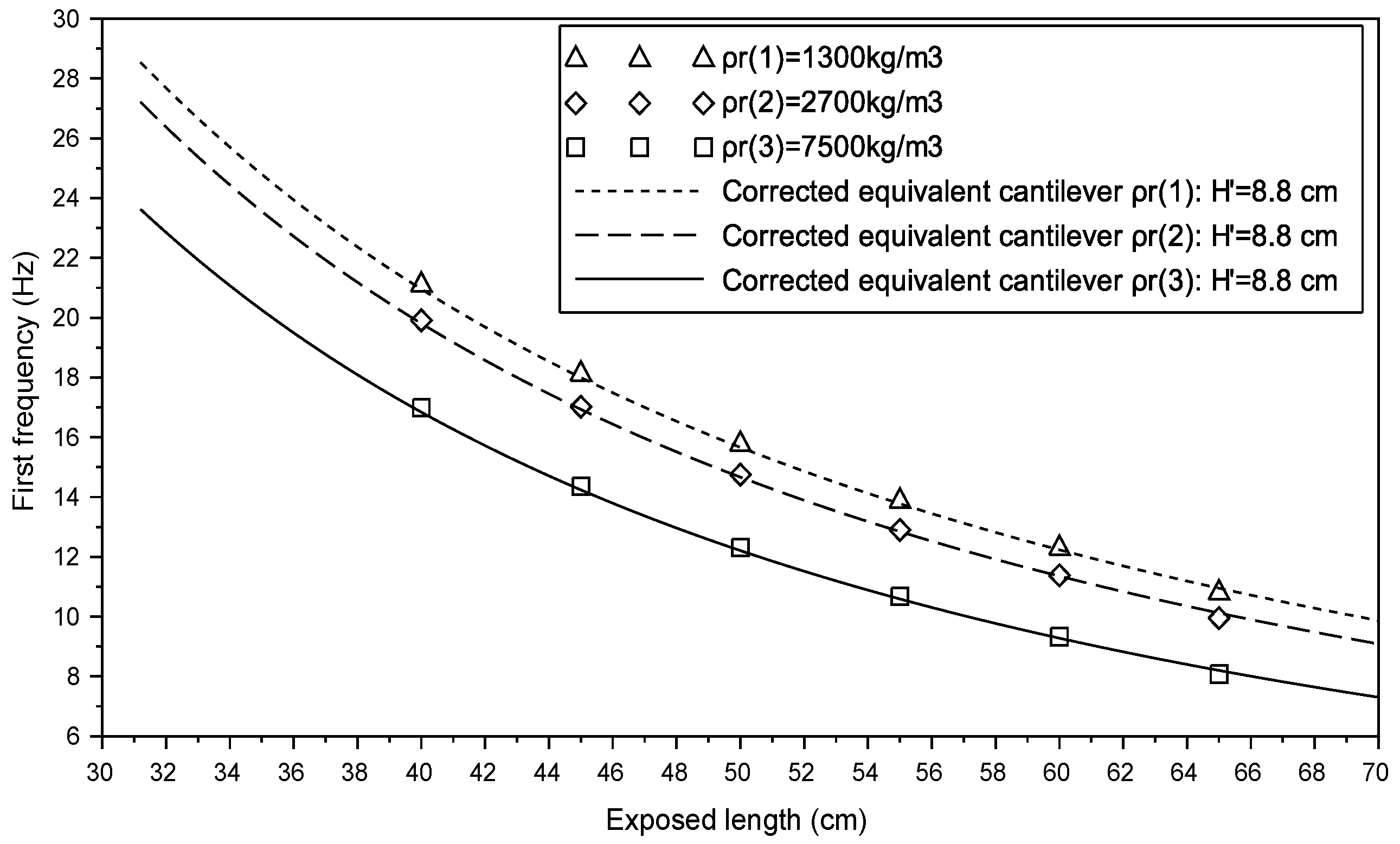
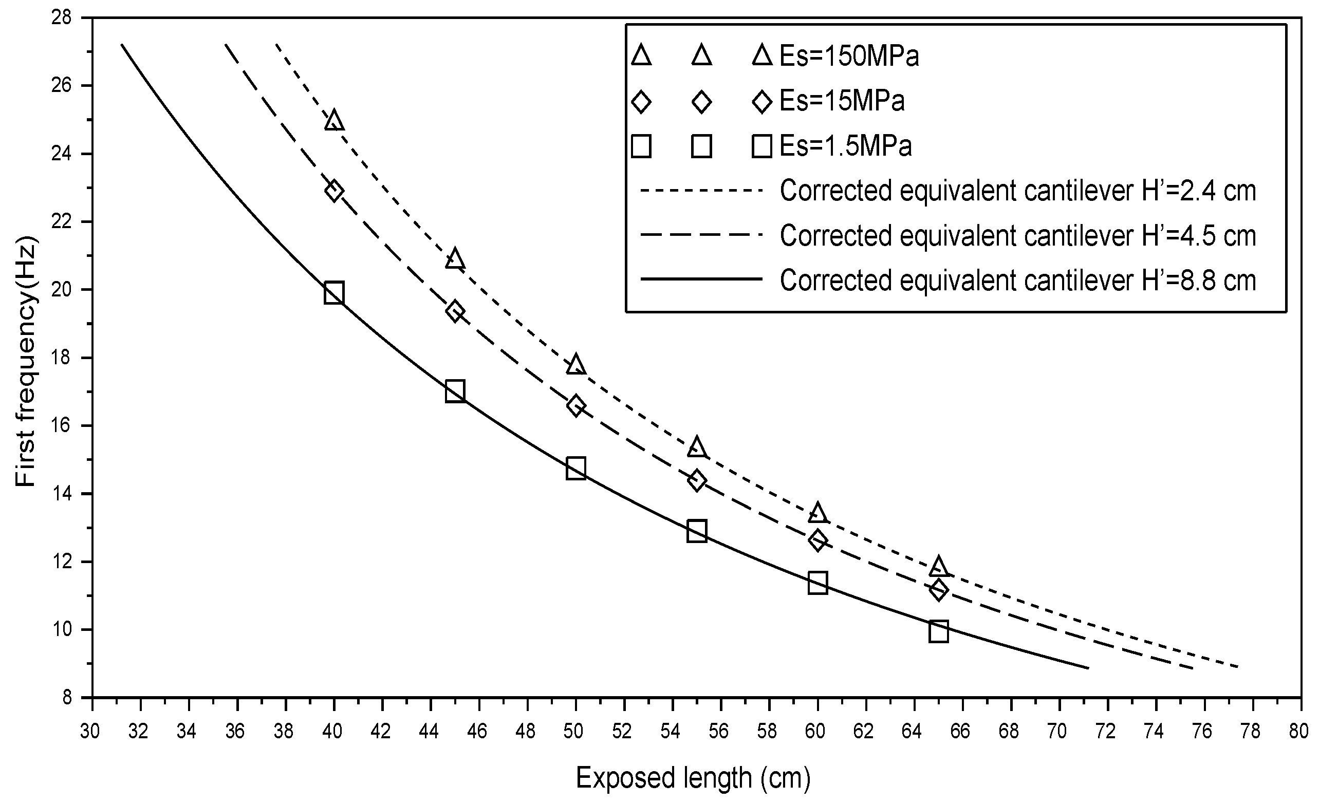
Finally, based on the experimental and numerical results, a simplified cantilever model with an increased exposed length was proposed to correlate the exposed length of the sensor to the measured frequency. This ‘correction’ of the free length of the cantilever varies with both soil and sensor characteristics. This correction length can be estimated while installing the sensor by calculating the frequencies of different exposed lengths. The proposed cantilever model is of practical interest since it is easier and quicker to implement to estimate scour depth with acceptable accuracy compared to the use of a beam-spring numerical model. Future research will focus on developing equations to calculate the ‘correction’ of the cantilever model for different sensor materials and soils and on large scale implementations of this monitoring technique.