Detecting Piping Failure in Levees Using Soil Moisture Propagation Mapping and a Wireless Sensor Network

Abstract

Earthen levees are crucial flood defense systems but are susceptible to failure due to internal erosion and saturation-induced instability, potentially causing breaches and endangering lives, infrastructure, and ecosystems in protected areas. Understanding soil saturation dynamics is vital for improved monitoring and resilience. This study presents a novel method of levee health monitoring by deploying a wireless sensor network consisting of nine small sensing spike packages with long-term UAV-deployability potential. In-package pressure, temperature, humidity, and—most importantly—soil conductivity are all measured by the suite of environmental sensors integrated into each spike package. This integrated sensing capability gives spatiotemporal information about the embankment’s subsurface moisture conditions. A 2 m long, 1 m wide, and 0.45 m tall sand-filled embankment replica was built for a controlled flume experiment to verify the system, enabling close examination of moisture permeability and propagation. The deployment of cutting-edge analytical methods for data interpretation is one of this study’s main contributions. Discrete conductivity measurements were converted into continuous, two-dimensional maps of moisture propagation using interpolation techniques, namely radial basis function (RBF). This makes it possible to see the changing moisture front inside the embankment structure in detail. Important information about early warning signs of possible instability (piping failures) is provided by this combined analytical framework. Using a network of nine wireless sensing spike packages, the proposed framework monitored moisture propagation within a 2 m long earthen embankment over a 105 min lab experiment and identified resistance changes associated with piping-like seepage behavior at approximately 19 min and 34 min, which exited approximately 10 min after detection. However, only seven of the nine packages produced viable readings. Improving flood risk forecasting models, improving infrastructure health monitoring applications, and guiding the development of more resilient levee systems are all directly impacted by this. This study demonstrates the potential in autonomous levee monitoring and management given that it combines robust spatial analytics and an interpolation method with inexpensive, quickly deployable sensing technology.

1. Introduction

Levees are artificial barriers, typically constructed from compacted soil, that run alongside rivers or coastlines. These elongated earthen structures play a vital role in flood protection by containing high water levels and preventing overflow into nearby communities, infrastructure, and agricultural land [1]. To remain effective, levees require regular monitoring and maintenance. Continuous monitoring and advanced data analytics [2] can reduce flood risk by enabling early warnings and timely preventative interventions [3,4]. Failures of these critical structures, often referred to as breaches, can result from excessive hydraulic pressure, internal erosion due to seepage, or structural damage from seismic events [5,6]. A vital levee failure mechanism, internal erosion (or piping), occurs when force from water seepage progressively moves soil particles. 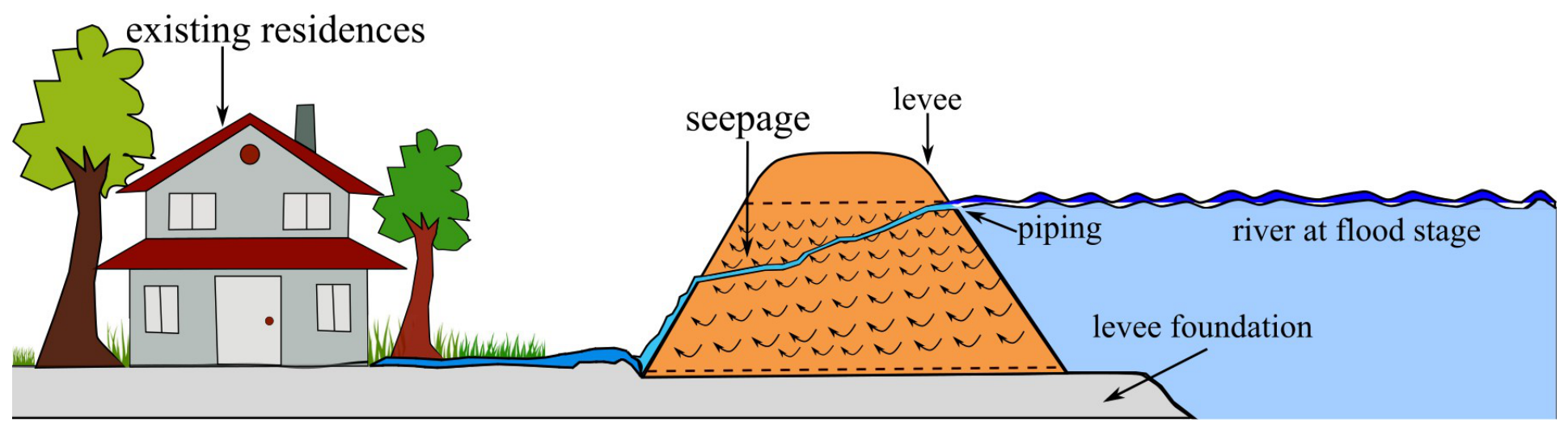This process creates subsurface channels, potentially leading to sand boils and structural collapse [7]. Contributing elements like animal burrows and decomposing root systems can accelerate internal erosion by creating preferred pathways for water infiltration. Seepage through, beneath, or along the levee foundation can undermine structural stability and increase the likelihood of failure during flood conditions, as shown in Figure 1.

Soil moisture is a primary driver of soil strength and stability, directly influencing deformation and failure behavior. Soil strength and deformation susceptibility are greatly influenced by this water content. In-ground sensors, satellite imagery, and geophysical surveys are just a few of the technologies scientists and engineers use to gather real-time soil moisture data across different time periods and locations [8]. In addition to reducing geological hazards like landslides, subsidence, and soil erosion, this information is crucial for managing water resources and improving agricultural practices. Professionals can gain important insights into the mechanical properties of soil by accurately assessing its moisture levels [9]. With this knowledge, geologists and engineers can more accurately forecast possible ground movement and put safeguards in place for communities and infrastructure. Geotechnical and environmental science continues to make significant strides thanks to extensive research on soil moisture monitoring techniques, applications, and significance [10].

Wireless sensor networks (WSNs) are a significant advancement in environmental data acquisition, especially in remote or challenging environments [11]. The wireless sensing spike network is an innovative method for assessing soil quality, consisting of numerous small, battery-operated sensor nodes distributed across a target area. These nodes collect environmental parameters like temperature, humidity, and pressure within the package body, which are then wirelessly transmitted to a central hub for continuous, large-scale monitoring. WSNs are useful for applications such as precision agriculture, environmental monitoring, and soil saturation in inaccessible regions. Wireless sensing spikes, which can directly collect and transmit data regarding soil attributes, eliminate the need for manual data collection and reduce time and labor demands. The development of compact drone-deployable sensors presents a more efficient and cost-effective approach for evaluating critical infrastructure and understanding soil health [12].

Spatial mapping of soil parameters is a crucial technique for understanding the spatial heterogeneity of soil properties across a landscape. This involves collecting data on various soil characteristics, including pH, organic matter content, and nutrient availability, at discrete locations within a defined area. Utilizing geostatistical methods such as kriging or regression analysis, researchers can then interpolate these point measurements to generate detailed maps illustrating the spatial distribution of these parameters [13]. This approach is invaluable in diverse fields like agriculture, land management, and environmental modeling, offering a comprehensive understanding of the complex relationships between soil properties, such as moisture levels, and other environmental variables. Otherwise, on a more accessible scale, radial basis functions (RBFs) offer simpler yet similar subsurface interpolation. Recent advancements in this area include the use of wireless sensor networks with conductivity probes for real-time soil saturation assessment in levees [14], and the application of UAV-deployed smart penetrometers for classifying soil saturation levels [15]. Published research in this domain frequently highlights methodological innovations and presents case studies showcasing the application of spatial mapping techniques in various geographical contexts [16].

Water’s electrical conductivity (EC) is a measurement of its electrical current-passing capacity. There are two possible causes for this: temperature and salinity level. As either increases, conductivity rises. Inorganic chemicals are more charged than organic ones, which is why salinity affects conductivity [17]. Temperature has an impact on conductivity because molecules can dissociate and ion mobility rises proportionately as liquid viscosity falls [18]. To forecast levee breakdowns and track their general health, electrical conductivity sensors are a good choice. The amounts of conductive chemicals in outdoor water sources are higher than those in purified water, making them measurable.

In this work, a wireless sensing spike package provides a novel framework for real-time monitoring and mapping of soil moisture propagation in levee embankments. A wireless network of nine autonomous sensing spike packages was developed, each equipped with soil conductivity sensors, onboard processing, data storage, power management, and wireless communication, enabling rapid UAV-based deployment and direct in-situ monitoring within levee structures. The contributions of this work are twofold: first, a self-contained electrical conductivity sensor package is introduced for levee structural health monitoring; second, the introduced sensor is experimentally evaluated on a lab-scale embankment for detecting moisture and seepage progression associated with piping-like failure.

2. Materials and Methods

This section outlines the hardware developed for this project before presenting the experimental validations undertaken and the data processing techniques utilized.

2.1. Hardware Development

The hardware developed for this experiment builds upon prior work on sensor packages [17] and their wireless versions [14]. It consists of two main components: a wireless sensing spike package and a receiver for data collection. These designs are open-source and available in the public GitHub repository under Columbia v0.6.0 [19].

2.2. Wireless Sensing Spike Packages

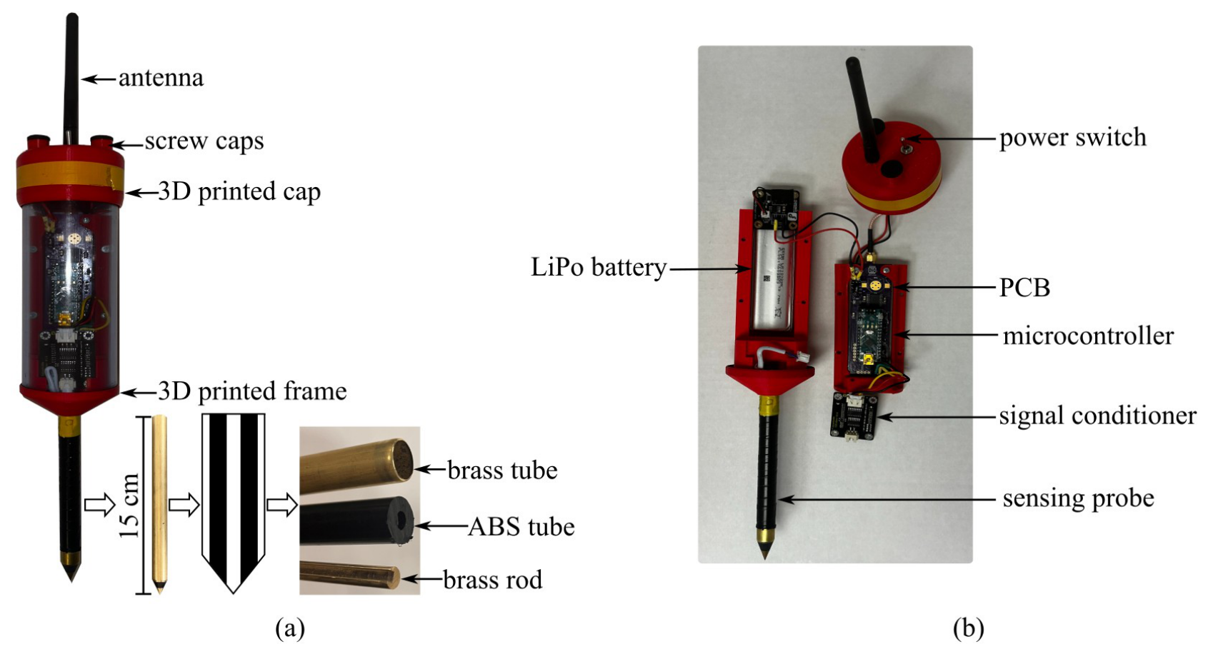
The sensing spike incorporates conducting elements—an outer brass tube and an inner brass rod—separated by an insulating ABS impact-resistant tube (Figure 2a). The total length of the spike is about 15 cm. This configuration enables the integration of a conductivity module at the spike tip, allowing the device to function as an underground moisture probe. Electrical tape wraps the outer layer, leaving only the tip exposed, thus enabling localized data acquisition. The ABS tube is pressure-fitted to ensure insulation and prevent electrical interference, providing a consistent reference for conductivity measurements. A total dissolved solids (TDS) module captures these measurements; it is encased in the package body and positioned just above the spike.

Encasing the sensing components is a transparent PVC pipe, approximately 5 inches long, which shields internal electronics while allowing visual inspection (Figure 2a). The PVC cover provides waterproofing via tight tolerances and rubber O-ring seals.

The internal layout of the sensing package is shown in Figure 2b. Housed inside the protective tube are a 3.7 V 3700 mAh LiPo battery, a power switch, and a printed circuit board (PCB). The system is controlled by an ATmega328P microcontroller chip. Alongside the TDS module, the package includes an nRF24L01+ PA/LNA RF transceiver module for wireless communication. This module features an external antenna, enabling communication distances of up to 1000 m in unobstructed conditions and offering enhanced signal integrity with the power amplifier (PA) and low-noise amplifier (LNA). An onboard BME280 sensor records ambient temperature, pressure, and humidity inside the housing; it is not intended to directly measure environmental conditions outside the package but rather to act as an internal reference point to external conditions and readings.

2.3. Receiver Data Collection

Figure 3 shows the overall wireless communication of a network of sensing spike packages. A single wireless sensing spike package is shown in Figure 2 reproduced for a total of nine nodes. Figure 3a is a network of nine wireless sensing spike packages. Each node must be given an address for proper communication over the ISM band, which is commonly used by WiFi and other Bluetooth devices. Each sensing package includes one RF module. Communication is facilitated via a star network configuration using the nRF24’s octal architecture, which supports six data pipes per module—ideal for coordinating multiple spike packages. The receiver station, as shown in Figure 3c, includes an ATmega328P microcontroller chip and a laptop with internet access for data collection and monitoring.

2.4. Individual Node Code Logic

The node measures soil electrical conductivity (EC) using a total dissolved solids (TDS) meter, which operates by emitting an AC excitation signal through one probe contact (via an oscillator and operational amplifier). This signal travels through the soil medium and is received at a second contact, effectively treating the soil as a resistive element. Together with a known resistor and an inverting op-amp configuration, the probe forms an amplifier circuit. As the soil resistance changes, the gain of the inverting amplifier varies accordingly.

This AC signal is then passed through a rectifier circuit, converting it to a DC voltage. The resulting DC voltage is proportional to the resistance of the soil, which allows for the calculation of EC since resistivity is the inverse of conductivity. Once this voltage is read by the microcontroller’s analog-to-digital converter (ADC), it is converted to a voltage value using the formula:

$$V={\displaystyle \frac{\mathrm{ADC}\mathrm{reading}\times 3.3}{1023}}$$

(1)

Here, 3.3 V is the supply voltage, and the ADC has a 10-bit resolution (a value range from 0 to 1023). This method is preferred over traditional DC voltage divider configurations because the AC signal prevents probe polarization and electrolysis, significantly extending the probe’s operational lifespan.

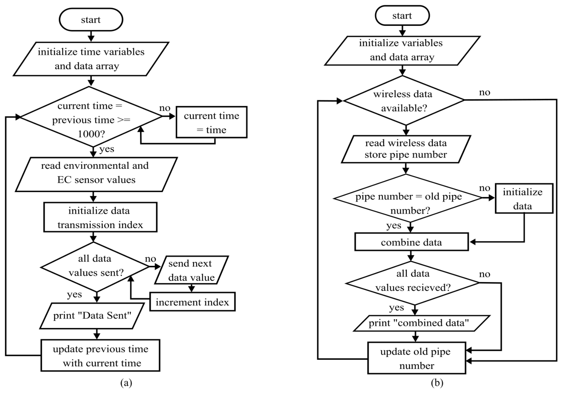
As outlined in Figure 4a, the program begins by initializing time-related variables and a six-element data array, combData[]. The variable current time holds the current system time in milliseconds, while the previous time stores the time of the last successful data collection and transmission.

The system continuously checks whether the difference between the current time and the previous time is greater than or equal to 1000 ms (i.e., 1 s). If not, it updates the current time and rechecks the condition. If the condition is satisfied, the node proceeds to read values from both the environmental sensor (BME280) and the EC sensor.

Once the readings are captured, they are stored sequentially in the combData[] array, including the node’s unique ID, timestamp (in seconds), temperature, humidity, pressure, and EC voltage. The code then initializes a transmission index and sequentially sends each value over the RF network. After all values are transmitted, the system prints “Data Sent” and updates the previous time to the current time, restarting the cycle.

This time-driven loop allows the user to easily modify the data transmission interval by changing the threshold comparison value, providing flexibility in data collection frequency. To ensure the node sends data immediately upon startup, the current time is initially set to a value greater than the threshold, and the previous time is set to zero.

To collect data, the node is instructed to take readings from the BME280 sensor and the A0 analog pin. The BME280 sensor measures the ambient temperature, humidity, and pressure inside the package, and the A0 analog pin measures the external electrical conductivity from the probe sensor. Once the data values are collected, the values are stored in their respective index within the combData array: the node number is stored in index 0, the current time is stored in index 1, the ambient temperature is stored in index 2, the humidity is stored in index 3, the pressure is stored in index 4, and the electrical conductivity is stored in index 5. The stored current time (in milliseconds) is divided by 1,000,000,000 to keep the value from becoming too large and prolonging runtime, since the function has a limited time range; the user’s desired time must be converted during post-processing. The electrical conductivity value is multiplied by 3.3 and divided by 1023 to convert the read ADC value to its equivalent voltage value. The 3.3 represents the voltage supplied to the electrical conductivity sensor, and 1023 represents the number of possible values for a 10-bit ADC minus one. The local variable i is created to represent the index of the combData array and is initially set to zero. The next condition evaluates if i is greater than 5. If false, the value stored in the corresponding index of the combData array is sent wirelessly to the receiver, and i is increased by one. If true, a “Data Sent” string is printed, the time is stored in the previous time variable, and the code returns to the first condition.

2.5. Receiver Code Logic

Based on the updated flowchart (Figure 4b), the receiver code initializes the following variables: an index i to 0, an array ‘combData’ of size 6 to store received data, the current transmitting node’s address ‘pipe number’ to 0, and the previous transmitting node’s address ‘old pipe number’ to 0. The receiver then enters a loop to continuously monitor for incoming wireless data. If no wireless data is currently available, the receiver remains in this checking state. Once wireless data is detected, the receiver reads the data and retrieves the network address (‘pipenumber’) of the sensor node that sent the data. Next, the receiver compares the current ‘pipe number’ with the ‘old pipe number’. If these values are different, it indicates that data is being received from a new sensor node, and the index i is reset to 0. This step is crucial for organizing data correctly, especially if data packets from different nodes arrive out of sequence or if there are transmission interruptions. The received data value is then stored in the ‘combData’ array at the position indicated by the current value of the index i, and subsequently, i is incremented by one. The receiver then checks if the index i has exceeded 5. If i is not greater than 5, it means that not all six expected data values have been received yet, so the receiver goes back to check for more incoming wireless data. Once i becomes greater than 5, it signifies that a complete set of six data values has been received. At this point, the receiver prints the values stored in the ‘combData’ array, from index 0 to 5. After printing the data, the index i is reset back to 0, and the ‘old pipe number’ is updated to the value of the current ‘pipe number’, preparing for the reception of data from the same or a different sensor node in the next iteration of the loop.

2.6. Experimental Setup

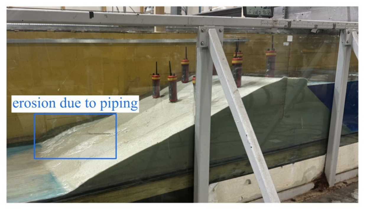
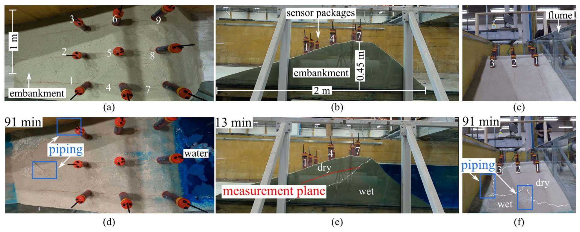
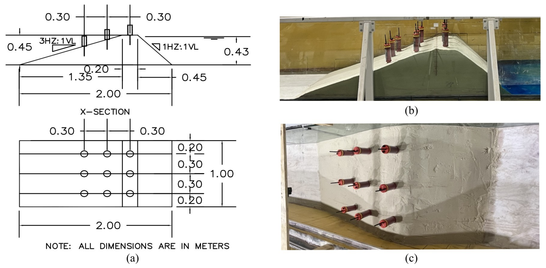
Figure 5 and Figure 6 illustrate the laboratory setup designed to test the wireless communication of sensing spike packages for the determination of soil moisture conditions within an earthen embankment. The experimental flume houses a constructed embankment measuring 2 m in length, 1 m in width, and 0.45 m in height. This embankment features asymmetrical slopes: a steeper 1:1 slope on the water-facing side and a more gradual 3:1 slope on the left side. 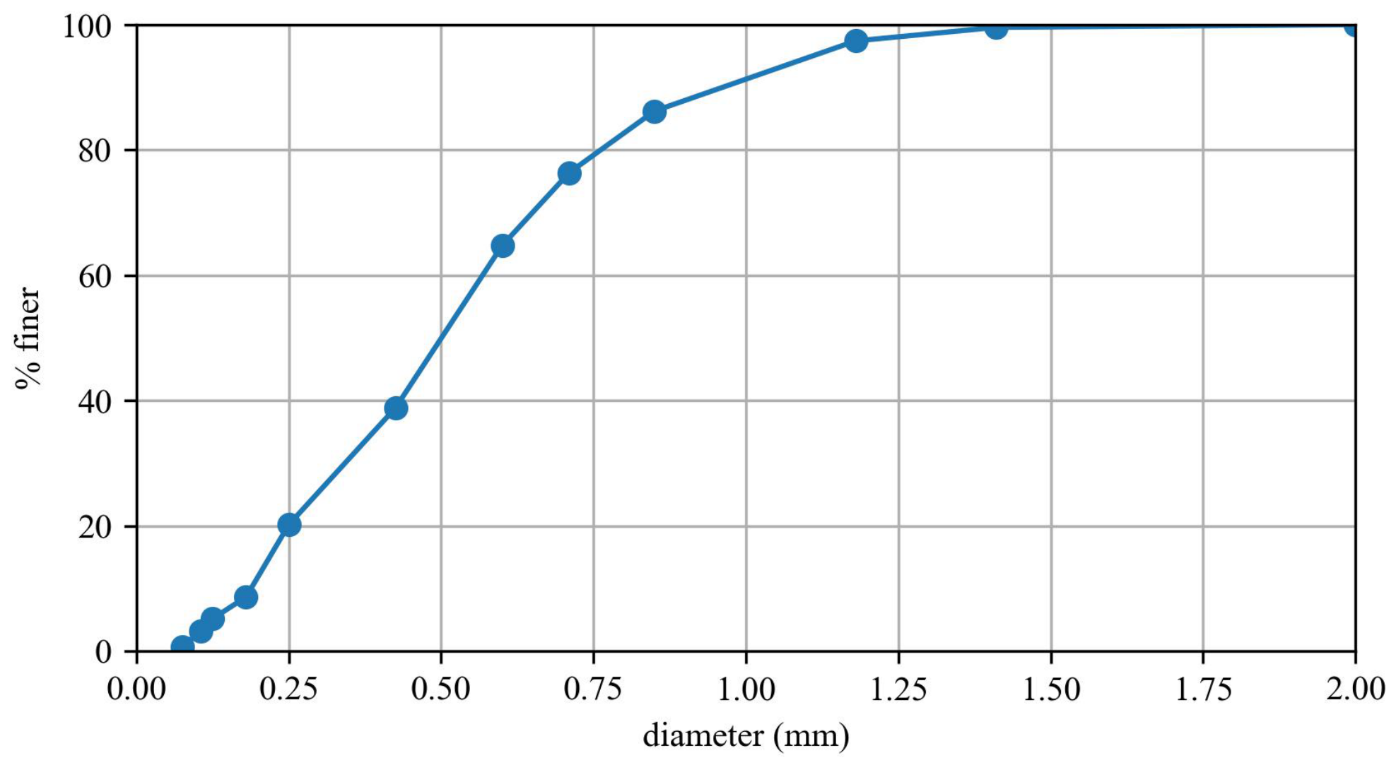A detailed layout of the proposed implementation of the earthen embankment is given in Appendix A and Figure A1. To simulate a body of water and induce moisture propagation within the embankment, the right side of the flume is filled with water. Additional information regarding the geotechnical properties of the sand, initial water content, and embankment preparation and compaction procedures is provided in Appendix B.

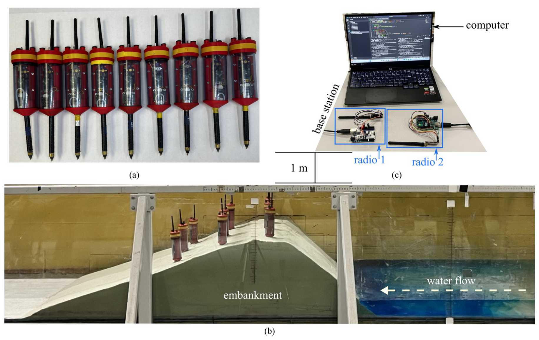
The base station, responsible for receiving and processing data from the wireless sensor network, is situated approximately 1 m away from the flume setup, as detailed in Figure 3b,c. A network of nine wireless sensing spike packages is deployed within the sandy material of the embankment, with their spatial arrangement visualized in the top, side, and front views presented in Figure 5a–c, respectively, under conditions of no direct moisture contact. For exact coordinates of each sensor node, please refer to

Table 1. Coordinates for the positions of nine wireless sensing spike packages.

Spikes	Notation of Fixed Resistor with Respect to the Spike	x-Coordinate (m)	y-Coordinate (m)	z-Coordinate (m)
1	$r_1$	0.85	0.2	0.25
2	$r_2$	0.85	0.5	0.25
3	$r_3$	0.85	0.8	0.25
4	$r_4$	1.15	0.2	0.35
5	$r_5$	1.15	0.5	0.35
6	$r_6$	1.15	0.8	0.35
7	$r_7$	1.45	0.2	0.45
8	$r_8$	1.45	0.5	0.45
9	$r_9$	1.45	0.8	0.45

. Subsequently, Figure 5d–f illustrate the progression of moisture induced by the water source, again shown in top, side, and front perspectives. Figure 6 reports an angled view of the test setup.

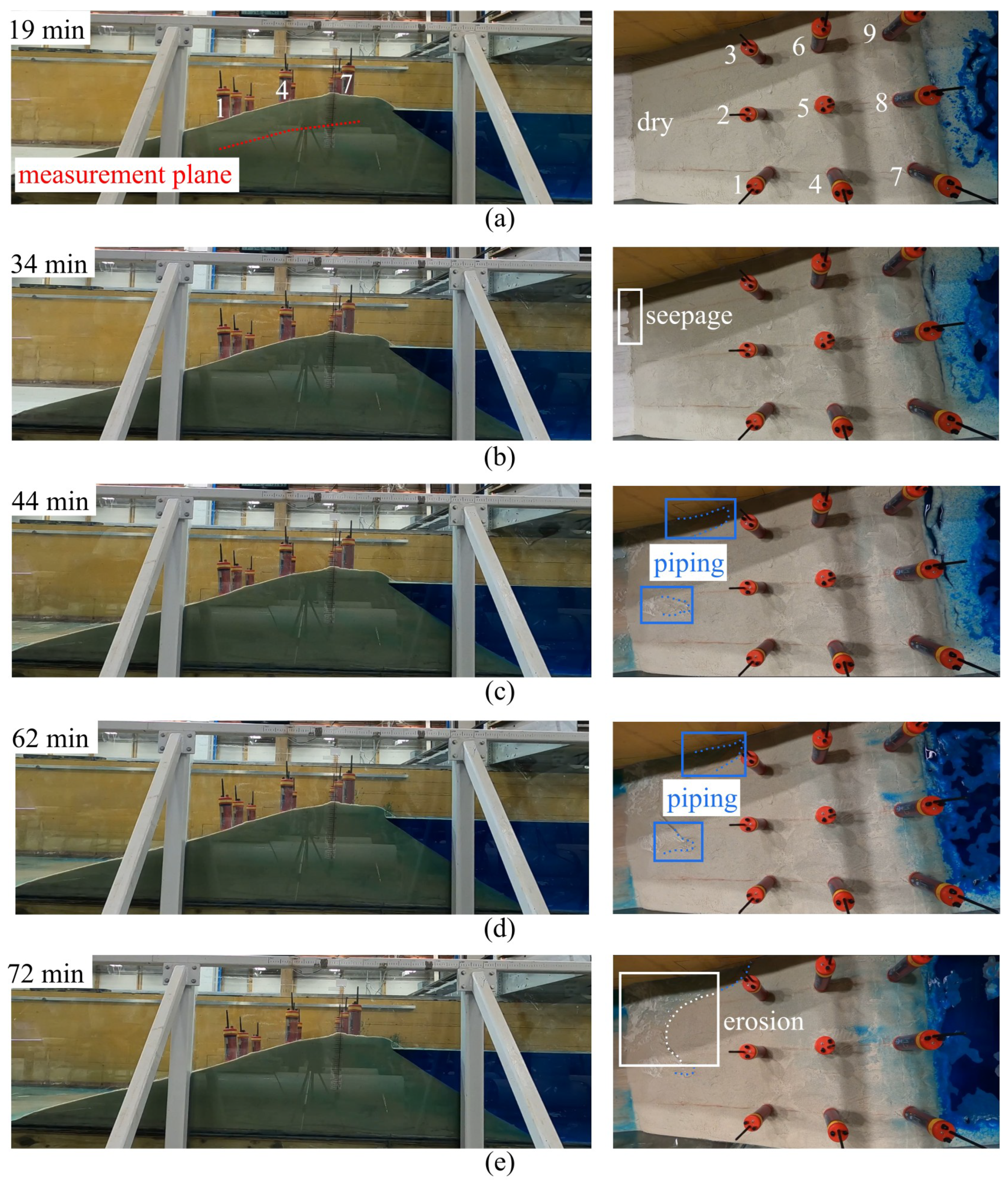
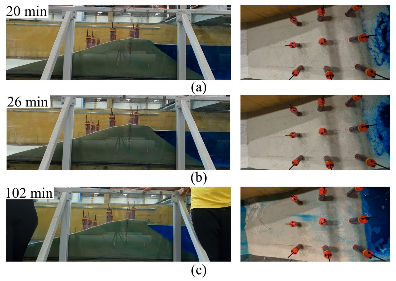
To ensure a comprehensive evaluation of the sensing spike packages’ performance over time and to visually track the spread of moisture, cameras are strategically positioned to capture top, side, and front views of the experimental setup throughout the duration of the experiment. The total runtime for this experimental phase was recorded as 105 min (1 h and 45 min). Figure 7 presents representative snapshots of the experimental configuration at multiple timestamps during moisture propagation, illustrating the spatial progression of saturation relative to the locations of the wireless sensing spike packages.

Figure 7. Visuals of the physical embankment from the side and top profiles at (a) 19 min, (b) 34 min, (c) 44 min, (d) 62 min, and (e) 72 min, complementary with Figure 8 and highlighting physically-observable phenomena.

Figure 7. Visuals of the physical embankment from the side and top profiles at (a) 19 min, (b) 34 min, (c) 44 min, (d) 62 min, and (e) 72 min, complementary with Figure 8 and highlighting physically-observable phenomena.

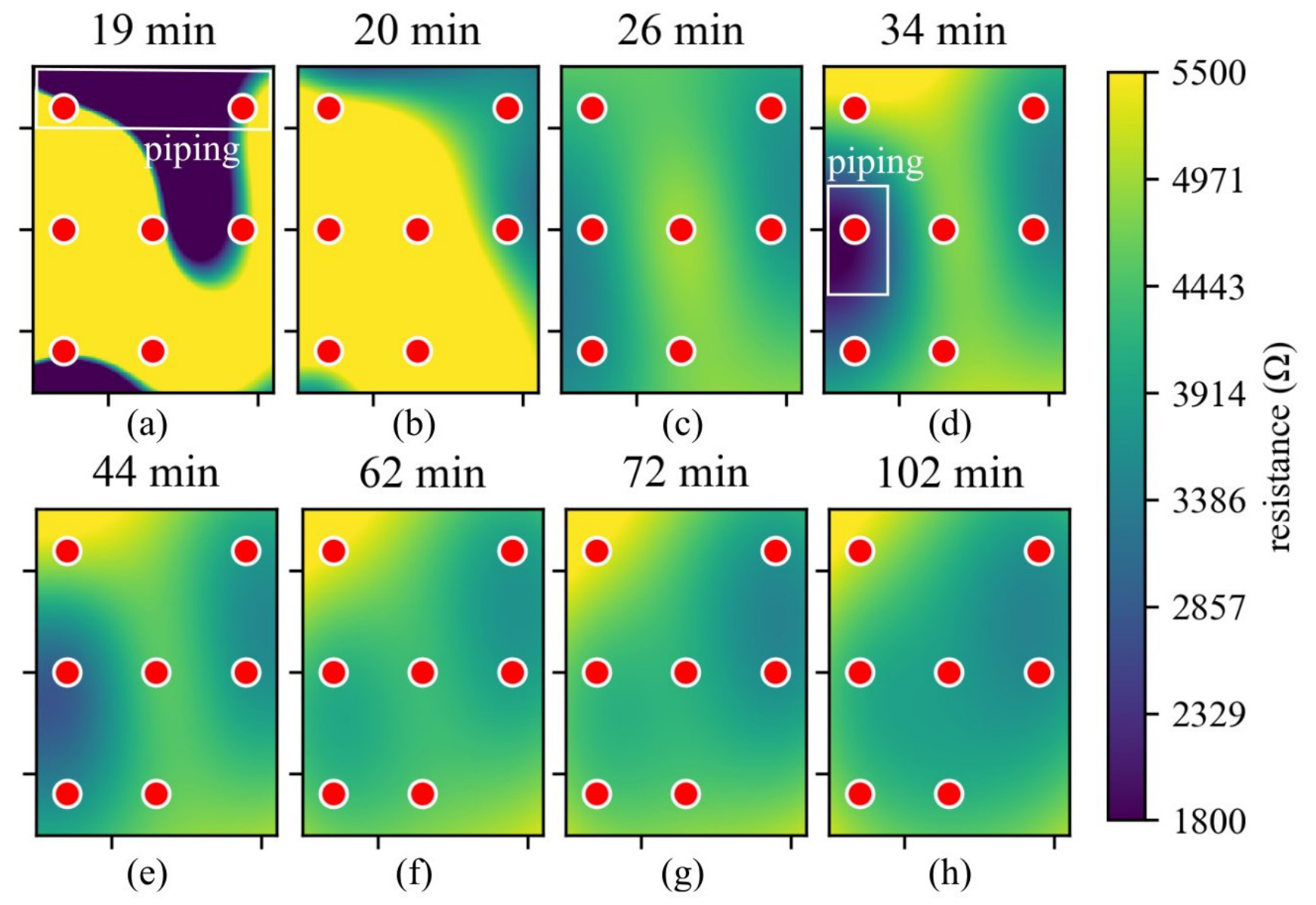
Figure 8. A series of RBFs along the measurement plane shown in Figure 5e at eight different timestamps that highlight the progression of two piping failures, which were initially detected at (a) 19 min and consequently at (d) 34 min. Timestamps (b,c) show a gradual increase in moisture across the entire plane before the second piping-like detection, while timestamps (e–h) show further increase across the plane after piping.

Figure 8. A series of RBFs along the measurement plane shown in Figure 5e at eight different timestamps that highlight the progression of two piping failures, which were initially detected at (a) 19 min and consequently at (d) 34 min. Timestamps (b,c) show a gradual increase in moisture across the entire plane before the second piping-like detection, while timestamps (e–h) show further increase across the plane after piping.

2.7. Data Processing

The experimental dataset and media collected, processed, and used in this paper is available in the public GitHub repository under dataset-1 [20].

To characterize changes in the electrical response associated with moisture propagation, sensor voltage measurements were converted to resistance during post-processing. Resistance is inversely related to electrical conductivity. The custom sensing spike configuration was previously characterized using an empirically determined voltage-to-electrical-conductivity relationship [21]. In this study, the voltage readings from each of the seven wireless sensing spike packages were processed as follows: The measured voltage, V, was first converted using the TDS sensor response function [22],

$$\mathrm{TDS}\left(V\right)=0.5\left(133.42V^3-255.86V^2+857.39V\right).$$

(2)

Using a TDS-to-conductivity conversion factor of 0.5, electrical conductivity is related to TDS as $EC=2\mathrm{TDS}$, where $EC$ is expressed in $\mathsf{\mu }\mathrm{S}/\mathrm{cm}$. Resistance was then estimated from electrical conductivity according to

$$R={\displaystyle \frac{K_{\mathrm{cell}}\times {10}^6}{EC}},$$

(3)

where $K_{\mathrm{cell}}=0.268{\mathrm{cm}}^{-1}$ is the estimated cell constant for the custom sensing spike geometry and R is expressed in ohms. Substituting $EC=2\mathrm{TDS}$ gives

$$R={\displaystyle \frac{500000K_{\mathrm{cell}}}{\mathrm{TDS}}}={\displaystyle \frac{134000}{\mathrm{TDS}}}.$$

(4)

This conversion was applied consistently to all sensing spike measurements and was used to evaluate relative changes in resistance associated with moisture propagation through the embankment. The resulting resistance values are interpreted as relative indicators of changes in local moisture conditions rather than as direct measurements of soil water content or degree of saturation. Because water content and degree of saturation were not measured sequentially during the experiments, a quantitative calibration between resistance and either parameter could not be established.

RBF interpolation is used to visually represent the moisture plane and its collected data; it is a method for approximating a function from scattered data by expressing it as a weighted sum of radially symmetric basis functions centered at the observed data points. Formally, the interpolant takes the form

$$f\left(x\right)={\displaystyle \sum _{i=1}^N}{w}_i\varphi (\parallel x-x_i\parallel )+P\left(x\right),$$

where $\varphi (·)$ is a radial kernel, $w_i$ are coefficients, and $P\left(x\right)$ is a low-degree polynomial included to ensure it is well-posed. SciPy’s RBFInterpolator library was used to create Figure 8, which specifically employs the thin plate spline (TPS) RBF by default [23], whose kernel is given by

$$\varphi \left(r\right)=r^{2}logr,$$

which was originally found as the solution to a variational problem that minimizes the bending energy of a surface subject to interpolation constraints [24]. This RBF choice produces a smooth interpolant that balances fidelity to the data with minimal curvature, making it particularly suitable for surface reconstruction, geometric warping, and spatial interpolation in two dimensions. Unlike kriging, which is a stochastic, model-based approach that incorporates an explicit covariance structure and provides uncertainty estimates, RBF interpolation is deterministic and does not require specifying a probabilistic model. Additionally, RBF methods differ from clustering techniques (e.g., k-means), which aim to partition data into groups rather than construct a continuous interpolating function. Thus, RBF interpolation, especially with thin plate splines, serves as a flexible and mathematically grounded tool for smooth function approximation from scattered observations [24].

The limited number of valid measurement locations introduces uncertainty in the reconstructed resistance field, particularly between sensor locations and near the boundaries of the measurement domain. Consequently, the interpolated maps are used primarily to visualize spatial trends supported by the nodal measurements rather than to resolve precise resistance values at unsampled locations. Interpolated features were therefore interpreted in conjunction with the individual sensor time series and physical observations of the embankment. Future work is needed to investigate denser sensor configurations and additional validation of the interpolation framework to better characterize and reduce uncertainty in the reconstructed resistance field.

3. Results

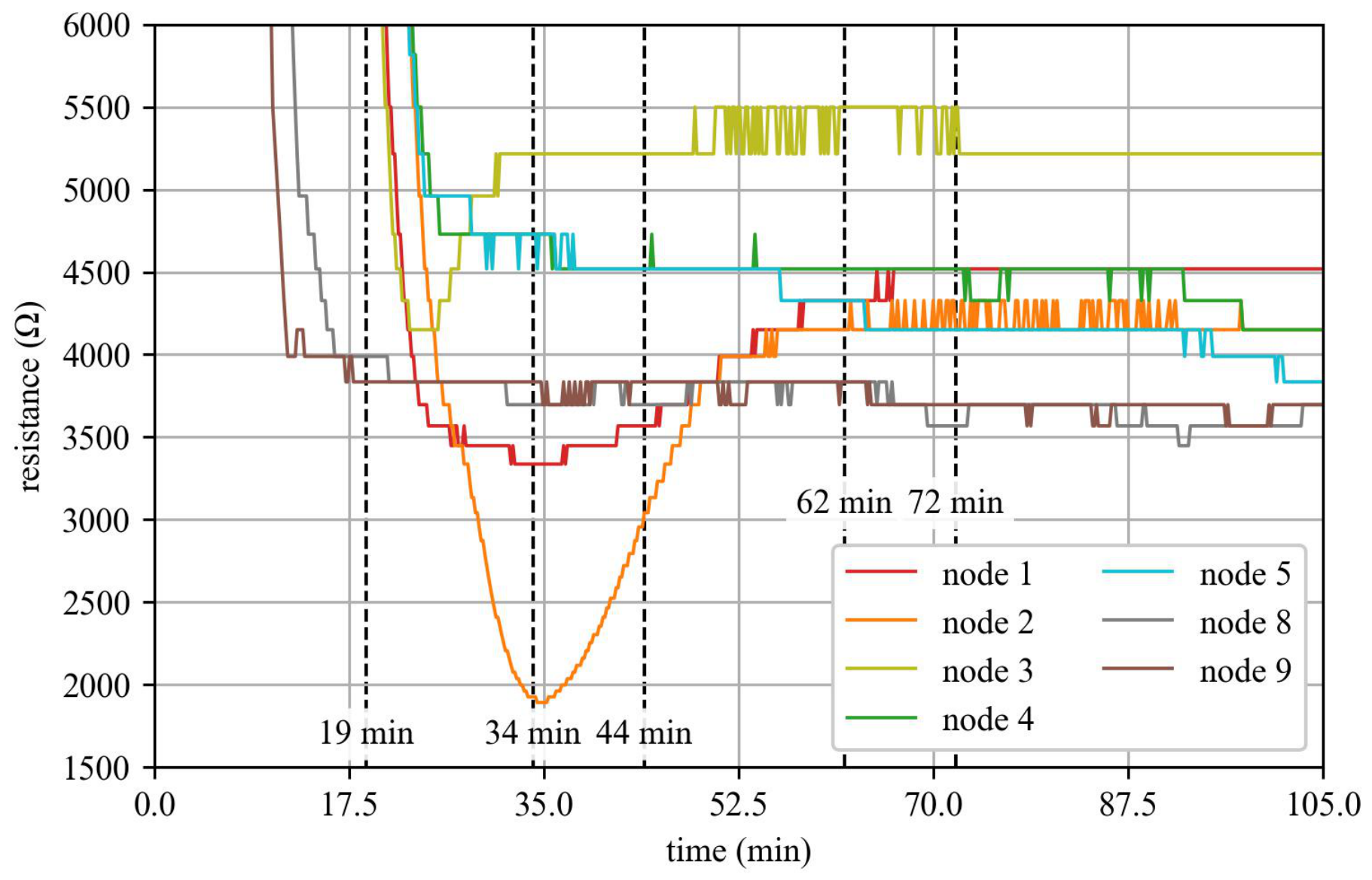
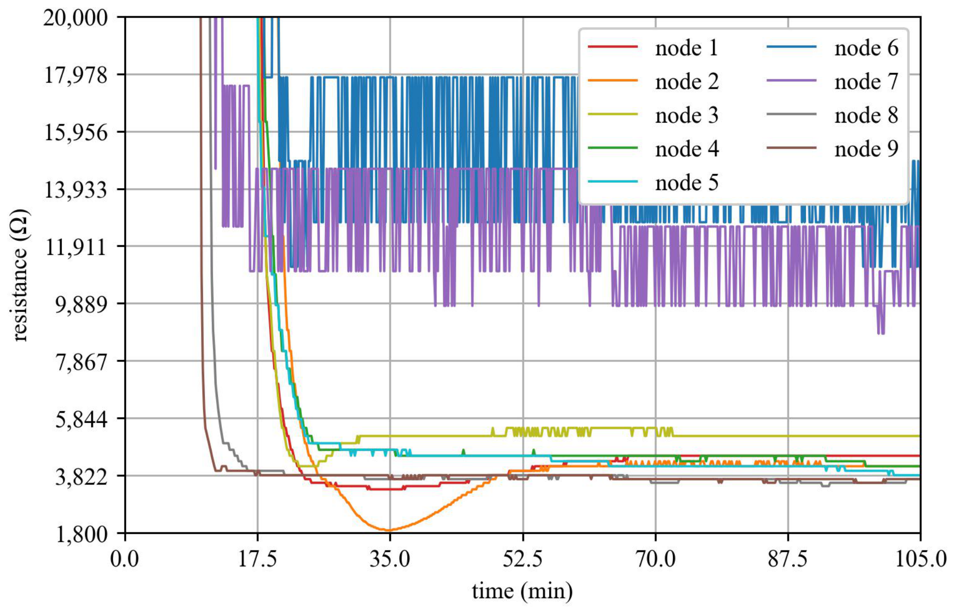
Resistance measurements from the wireless sensing network revealed progressive moisture infiltration throughout the embankment over the 105 min experiment, as shown in Figure 9, which captures the resistance responses from seven wireless sensing spike packages. Furthermore, Figure 9 depicts a general downward trend in resistance across the sensors, indicative of increasing moisture content at their respective sensing locations due to the inverse relationship between resistivity and conductivity. The variability in resistance responses across sensors suggests a spatially non-uniform moisture distribution within the test medium. In particular, nodes 2 and 3 exhibited substantially different resistance responses despite their proximity and equivalent installation depth. The larger resistance decrease at node 2 coincided with the location of the physically observed piping-like seepage pathway, suggesting highly localized moisture propagation within this region of the embankment.

Piping-like seepage behavior was detected at two distinct stages of the experiment using the interpolated resistance maps shown in Figure 8, with piping detected visually at approximately 19 min and again at approximately 34 min, signified by the dark blue-purple representation of recorded resistance nearing 1800 ohms. These identified failures coincide directly with the dips in resistance shown in Figure 9 and precede the visually observed erosion and piping-like exits shown in Figure 5, Figure 6 and Figure 7 by approximately 10 min.

The purple portion of the color range represents the lowest recorded resistance values and is therefore associated with the greatest relative increase in local moisture conditions. Water piping is considered the highest concentration of moisture due to the tunneling displacing sand rather than the lower concentration distribution of regular seepage. Decreasing resistance is associated with increasing local moisture conditions due to the naturally present ionic content of the pore water. However, resistance reduction alone is not enough to validate the occurrence of piping, which is why the path locations are cross-referenced between physical observations of the embankment (Figure 7), values recorded by each node (Figure 9), and the interpolated moisture map (Figure 8).

The RBFs in Figure 8 map along the measurement plane outlined in Figure 5e. The map starts with a primarily high overall resistance of over 5000 ohms shown in yellow, representing the relatively drier initial embankment condition. For the initial piping alongside the top edge of the embankment in Figure 8a, the blue-green lining of the 1800-ohm drop matches the progressing resistance drops shown in Figure 9 around that time. The same connection between matching time-series drops and the RBF color map appears for the piping in Figure 8d. From there, both the RBFs and the time series plateau until the end of the experiment, remaining in that midrange between 4500 and 3500 ohms, attributed to the water path usage of residual pathways and moisture spreading more evenly throughout the embankment.

The physically observed phenomena are delayed compared to the sensor data and moisture map. In Figure 7a, despite the 1800-ohm drop along the sides in Figure 8, the water has not yet reached the other side of the embankment, and it remains dry. It is not until 34 min (Figure 7b) that the water has seeped throughout the embankment, thus marking the start of the side piping’s exit, which is when the second piping is detected according to Figure 8d. It is inferred that the first failure occurred along the side because the sand against the wall is an easier edge to initially erode. By 44 min, it is observed in Figure 7c that both detected piping failures have broken through the other side of the embankment. From there, water continues to travel through the embankment along these piping paths, as shown by the resistance plateau at later timestamps in Figure 8. As the water continues to follow these piping paths, there is a gradual increase in erosion of the outer edge, visible in Figure 7e. Continued exposure to these conditions would be expected to progressively erode the embankment until it eventually collapses or breaks away. These observations demonstrate the sensors’ ability to detect changes associated with developing seepage pathways and support their potential for early identification of moisture propagation preceding piping-like failure.

The initial seepage pathway developed along the brick side wall of the flume, where the sand-brick interface and grooves in the wall may have provided a preferential flow path. These grooves could have facilitated concentrated seepage along the boundary, resulting in a piping-like pathway that may not represent true internal erosion piping within the embankment. Therefore, the initial observed failure cannot be conclusively distinguished from preferential boundary seepage. However, the interpolation in Figure 8 indicates that the associated moisture propagation was not confined to the brick wall and extended into the interior of the embankment. The sensing system captured the spatial progression of this wetting pathway; however, the present experiment does not establish whether an equivalent early sensor response would precede piping developing entirely within the embankment. Additional testing designed to minimize boundary effects is needed to evaluate the early-warning capability of the sensing system for internal erosion piping specifically.

Sensor inconsistencies in nodes 6 and 7 produced anomalous baseline resistance measurements that required their exclusion from the primary analysis due to differences in the conductivity sensor signal conditioner used in these sensor packages. While data from the other seven nodes were able to construct an accurate moisture map, this indicates that, in practical applications, the deployment of multiple spike sensor packages can be beneficial: overall moisture distribution can still be mapped accurately even if some spikes fail, as spatial interpolation can be performed using data from the functioning sensors. Still, more sensors would provide a validating comparison that would strengthen the initial framework.

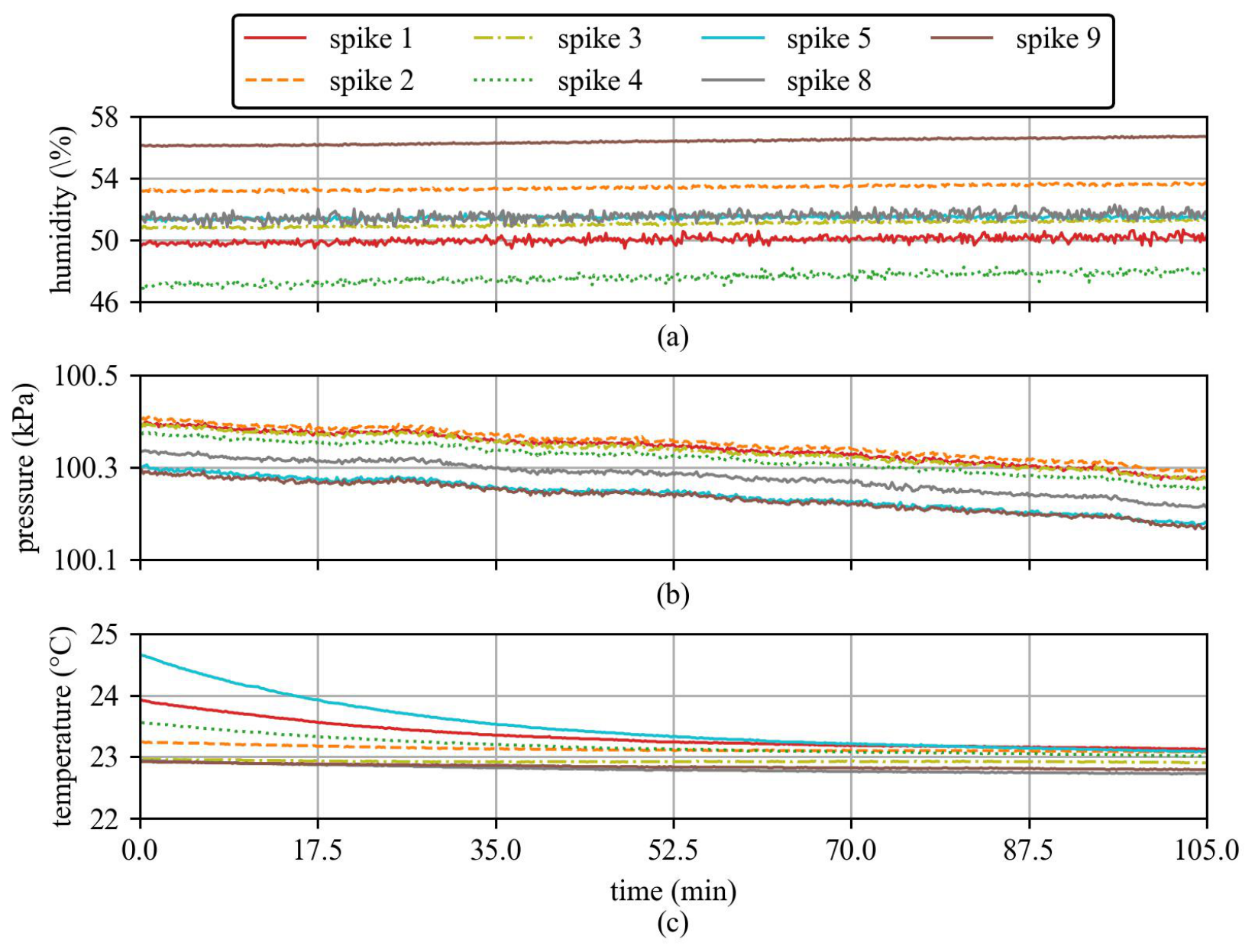
In-package environmental measurements from the onboard BME280 sensor provided additional context for interpreting changes in soil resistance throughout the experiment, as shown in Figure A4. Figure A4a shows a modest increase in relative humidity, while Figure A4b captures a gradual decrease in atmospheric pressure. Figure A4c illustrates a steady decline in ambient temperature over the test period, a factor known to influence soil electrical properties such as conductivity and permittivity, thereby potentially impacting sensor output. These environmental variables are essential for interpreting the sensor data, as they modulate the soil’s dielectric response and, consequently, the resistance measurements.

Combined temporal and spatial sensor measurements captured the evolving moisture transport behavior within the embankment under dynamic test conditions, highlighting the complex interaction between soil moisture dynamics and environmental factors. The complicated interaction between soil moisture dynamics and external factors is shown by the diverse resistance trends seen throughout the sensor network when combined with changing environmental scenarios. Analyzing the resistance’s spatial distribution could offer more information on the medium’s moisture progression.

4. Conclusions

This study introduces a novel approach to levee health monitoring, utilizing a wireless network of sensor spike packages that measure in-situ soil resistance as a proxy for moisture content. In a controlled laboratory setting, these nine sensor spikes are embedded within an earthen embankment model, of which seven provided viable resistance measurements for the primary analysis, with data collected over the course of 105 min. The resistance data undergoes processing via radial basis function for interpolation, facilitating segmentation of moisture conditions and detailed visualization of relative moisture zones over time.

The results demonstrate the preliminary feasibility of using distributed sensing and spatial interpolation to monitor non-uniform moisture transport and identify early indicators associated with internal erosion. Additionally, the ability to reconstruct spatial patterns associated with moisture propagation despite the exclusion of malfunctioning nodes suggests that the proposed sensing framework can maintain useful spatial information in the presence of individual sensor failures, supporting its potential for more robust distributed monitoring applications.

Overall, this work demonstrates the potential of low-cost wireless sensing systems for continuous levee health monitoring and early warning applications. Future work will focus on larger-scale deployments and field validation under realistic environmental conditions to further improve failure localization and predictive monitoring capabilities.