Article

Evaluating Seismic Source Effects on the Collapse Modes of Existing Curved Viaduct

School of Civil Engineering, Universidad Michoacana de San Nicolás de Hidalgo, Av. Francisco J. Múgica S/N, Morelia C.P. 58030, Michoacán, Mexico
*
Author to whom correspondence should be addressed.
Infrastructures 2026, 11(9), 332; https://doi.org/10.3390/infrastructures11090332 (registering DOI)
Submission received: 8 August 2026 / Revised: 12 September 2026 / Accepted: 15 September 2026 / Published: 19 September 2026
(This article belongs to the Special Issue Seismic Engineering in Infrastructures: Challenges and Prospects)

Abstract

Curved bridges subjected to strong ground motions have shown high seismic vulnerability in many countries. Several published studies analyze curved-bridge failures, focusing on collapses observed after severe earthquakes, which are frequently linked to loss of seating length. Other studies assess seismic fragility based on expected pier damage, and most published work uses numerical models derived from existing bridge portfolios that do not include specific real bridges. Many studies also aim to correlate the dynamic properties of existing bridges, estimated from ambient vibration measurements, with those of numerical models. The approaches mentioned above estimate the expected seismic response for specific bridge types that may not accurately represent real structures, and examine the most common failure mechanisms. Unlike these studies, the current research provides valuable and novel insights into the expected behavior of curved viaducts designed in accordance with modern standards and regulations. It shows that, in these cases, the most frequently reported failure in the literature, loss of seating length, is less likely than other failure mechanisms. The results apply to a real curved bridge whose numerical model was previously calibrated using ambient vibration measurements. Another distinctive feature is the assessment of reliability indices for a real structure, evaluating the values that current regulations would expect to observe during infrequent seismic events. Uncertainties in site amplification are reduced because a nearby seismic station is available. Nonlinear analyses were performed using two sets of seismic records from interplate and intraplate earthquake sources, scaled to match the expected seismic intensity at the bridge site, to assess damage progression in the bridge under both design and infrequent earthquake intensities. The study also emphasizes the significant effects of the selected ground-motion population and the frequency content of interplate and intraplate earthquakes on bridge seismic performance. Unlike the failure mechanism most commonly observed in curved bridges during high-intensity seismic events, which involves loss of superstructure seating length, this case study of a curved bridge designed under modern seismic regulations shows failure when shear demands exceed the bridge piers’ shear capacity.

1. Introduction

Curved and skewed bridges are more vulnerable to earthquakes than straight bridges. The Loma Prieta earthquake on 17 October 1989 (Mw = 6.9) caused significant damage to San Francisco Bay’s bridge infrastructure [1]. The authors noted that skewness was a crucial factor in the observed damage to bridges. Two of the three collapsed bridges were skewed.
Similarly, the Northridge earthquake on 17 January 1994 (Mw = 6.7) caused significant bridge damage and several collapses [1]. The damage assessment identified 233 damaged bridges across four counties. The collapsed Gavin Canyon Undercrossing Bridge 53-1797R had a 67-degree skew. Substantial displacement and rotational demands led to failure and loss of support [2]. The southbound separation and overhead viaduct at Route 14/I-5 (53 1960F) is a curved, 10-span, continuous concrete box girder bridge. It collapsed from abutment 1 to the hinge of span 3, possibly due to a loss of seating length. The North Connector (53 1964F) also collapsed. It is a curved structure with collapsed spans 1 and 2 and pier 2. The damage showed that at abutment 1, the most significant movement was in the bridge’s longitudinal direction. Although the loss of seating was also a possible cause of the failure, Buckle [2] suggested that pier 2 failed first because of the high shear demands on this short pier.
Wang and Lee [3] compared bridge damage and collapse modes from the Wenchuan earthquake with those observed in similar bridges during the Northridge, Loma Prieta, and San Fernando Earthquakes. Among the damage and failure modes, skewed or curved bridges, especially those with tall piers, should be avoided in high-seismic areas. The Wenchuan earthquake underscored the need to develop seismic design guidelines and strategies for bridges near faults, or even those crossing faults, to withstand enormous displacement demands.
Anderson et al. [4] showed that two skew bridges on the Meishin Expressway were damaged during the 17 January 1995, Kobe earthquake in Japan (Mw = 7.0), despite having been retrofitted. The non-skew spans did not fail during the earthquake. During the 12 May 2008, Sichuan earthquake (Mw = 7.9) in China, many bridges were damage [5,6,7]. The curved Baihua Bridge collapsed. According to Han et al. [5], several factors contributed to the collapse, including a lack of longitudinal and vertical displacement restraints, excessive seismic demands, and insufficient seat length, among others. The ramp bridge at the Huilan interchange sustained severe damage to the piers. The bridge consisted of curved, continuous box girders. Han et al. [5] identified insufficient transverse reinforcement as a potential cause of the observed damage at the pier tops.
Beyond post-earthquake case studies, several analytical studies have examined the seismic response of curved and skewed bridges. Wilson et al. [8] analyzed the combined effects of skew and curvature on bridges’ expected seismic performance. They observed significant superstructure deformations that further damaged the substructures. They also emphasized that skewed and curved bridges require detailed analytical modeling. Serdar et al. [9] and Serdar and Folic [10] highlighted the importance of deck radius in determining expected damages for curved bridges. Their findings indicated that curved bridges are prone to collapse under lower ductility demands compared to straight bridges.
Recent studies have employed loss models to assess the performance of curved bridges [11,12]. Specifically, Feng et al. examine how the spatial variability of earthquake ground motions influences the seismic response of these structures. They conclude that the impact of the angle of seismic incidence diminishes as seismic intensity increases, resulting in expected losses that are independent of this angle at high seismic intensities. Furthermore, the effects of seismic directionality on the seismic vulnerability of curved bridges have been studied, and it has been concluded that displacement demands may increase [13,14,15]. These studies also suggested using the SRSS rule and the spectral intensity at the dominant period to scale seismic records.
Some studies have examined how geometric parameters affect the seismic performance of curved bridges. Seo and Linzell [16] analyzed the seismic behavior of curved steel bridges to evaluate how different factors influence their response. The parameters studied included the number of spans (1–3), the radius of curvature, the maximum span length, the girder spacing, and the diaphragm spacing. Nonlinear dynamic analyses were conducted using El Centro ground motion records. The results revealed ductility demands in columns, significant deformations at the supports, and axial forces in the diaphragms, all indicating extensive damage. Based on the parametric analysis, the most critical parameters affecting the bridges’ seismic response were the number of spans and the radius of curvature.
Siami and Tehrani [17] used both linear and nonlinear analyses to assess the seismic performance of curved reinforced concrete bridges featuring various geometric irregularities. They compared these with equivalent straight bridges as recommended by AASHTO. The study analyzed 84 bridges in total, 12 straight and 72 curved, each with four spans and a total length of 160 m. The configurations included varying pier heights, span lengths, abutment support conditions (fixed or simply supported), and bridge subtended angles from 0° to 180° in 30° increments.
The findings showed small variation in displacement demands between linear and nonlinear analyses (up to 10%) for bridges with fixed abutments. However, the differences were much larger for bridges with simply supported abutments. Consequently, the authors recommended revising AASHTO guidelines to incorporate criteria addressing support conditions and the interaction of different irregularities in choosing the most suitable analysis method.
Heydarpour and Tehrani [18] studied 21 bridge models, each 160 m long, with a prestressed concrete box-girder superstructure and four equal spans. The authors found that curved geometry had minimal impact on the seismic response of bridges with free abutments. In contrast, when abutments interacted with the superstructure, curvature significantly affected displacements at both the piers and the abutments, particularly in the radial direction. Regarding the use of equivalent straight bridges, the authors recommended their use only for curved bridges with subtended angles less than 30°, as larger angles led to underestimating deck displacement demands in both directions.
Deshpande et al. [19] examined the influence of curvature radius and pier skewness on the seismic response of curved reinforced concrete bridges with two superstructure types: box girders and I-girders. The study modeled two-span bridges, each 50 m long, with pier skew angles of 0°, 15°, and 30°, radii of curvature of 150 m and 250 m, and a straight configuration. Modal analysis showed that as the radius of curvature increased, the bridge’s transverse vibration period decreased. In contrast, increasing the skew angle led to a longer transverse vibration period and a shorter longitudinal period. Additionally, pushover analyses showed that a larger radius of curvature led to lower base shear demands. The I-girder bridge was more flexible in both directions than the box girder bridge. At the same time, the latter demonstrated better expected seismic performance.
Amjadian and Agrawal [20] investigated the pounding between the abutments and the superstructure of curved bridges. The study focused on short-span bridges and assumed rigid-body behavior of the deck. The model integrated nonlinear contact behavior with the abutments and accounted for frictional effects. The authors examined parameters including span length, the subtended curvature angle, the gap between the deck and abutments, friction, and column stiffness. The results showed that seismic pounding causes significant displacements and rotations in the deck, even in symmetric structures. Additionally, friction played a dual role, either increasing or reducing the torsional response depending on the impact direction. Overall, the study found that the deck’s maximum displacements and rotations are highly sensitive to gap size and bridge curvature.
Regarding experimental studies, Banerjee and Shinozuka [21] conducted a full-scale experimental study that combined analytical and empirical methods to verify the damage limit states proposed in code provisions. They found good consistency among the empirical, analytical, and experimental results with the limit states defined by HAZUS. Sakai and Unjoh [22] conducted an experimental study of bridge column behavior under multidirectional seismic actions. They reported that the maximum demands were lower than the columns’ capacity because seismic demands, axial loads, and flexure never reached their maximum values simultaneously. Sun et al. [23] conducted an experimental study of three techniques for repairing circular bridge piers severely damaged by earthquakes. They concluded that the concrete jacket confined by CFRP sheets is the most effective under a flexural failure mechanism. Jiao et al. [24] conducted shake-table experiments on a 1:25-scale curved bridge model to study pounding between adjacent decks. The reference model consisted of two curved segments: a single-span bridge of 25 m supported at both ends, and a two-span continuous bridge with two end supports and one intermediate support, forming a three-span configuration with a radius of curvature of 75 m. The model was subjected to various ground motions, including pulse-like and far-field records, with joint openings ranging from 1 to 4 mm in the scaled model.
The results showed that the most unfavorable seismic excitation direction was aligned with the secant line connecting the two piers of the single-span deck and with the corresponding orthogonal direction. Pounding at the joint indicated that contact between the decks is not uniform, amplifying the rigid-body rotation of the curved bridge and consequently increasing its displacements. They concluded that joint size can help mitigate pounding effects, thereby reducing the rotational response of curved bridges.
The design philosophy within building codes has evolved over time. Currently, seismic design aims not only for minimum structural safety but also for structural resilience. According to Cimellaro, Reinhorn, and Bruneau [25], resilience is a normalized function that indicates the capacity of a building, bridge, lifeline, network, or community to maintain a level of functionality or performance over a specific timeframe (such as a life cycle or service life), including the recovery period following damage caused by an extreme event. A pioneering work on this topic is Bruneau et al. [26], who define community earthquake resilience as “the ability of social units (e.g., organizations, communities) to mitigate hazards, contain the effects of disasters when they occur, and carry out recovery activities in ways to minimize social disruption and mitigate the effects of further earthquakes”. This study proposes dividing resilience into four components: robustness, redundancy, resourcefulness, and rapidity. Various authors have proposed methodologies to evaluate one or more of these components, with particular emphasis on quantifying recovery times [27,28,29,30]. Research has also evaluated resilience in scenarios requiring structural repairs to buildings [31]. Studies that incorporate resilience as a fundamental parameter have found broad application beyond buildings or bridges alone [32,33,34]. Recent studies [35] have aimed to optimize intensity measures for seismic resilience, using an expression that depends on the recovery function and repair time.
The studies above show that various researchers have performed nonlinear parametric analyses of curved bridges using numerical models that incorporate different parameters, without using the geometric characteristics of any specific existing bridge [36,37,38]. Very few studies have focused on existing curved bridges, and even fewer have examined structures subjected to seismic records from two different types of seismic sources, each with an independent generation process, that can cause significant damage. Most of the studied bridges represent common typologies, and none of the research integrates analysis of recently built curved bridges with on-site seismic data to evaluate site effects. Additionally, quantifying the failure probability and reliability index of a real curved bridge designed to current seismic codes is fundamental to properly assess its safety.
Estimating bridges’ seismic vulnerability often involves sets of accelerograms that include only interplate earthquakes or, at times, a combination of seismic records from interplate and intraplate sources. Both seismic sources have damaged buildings and bridges in Mexico. They exhibit independent occurrence processes, and both can produce strong earthquakes. Because the occurrence processes and source locations are independent (one on the Pacific coast and the other inland), evaluating bridge seismic vulnerability requires separate seismic records for each source. Although seismic regions worldwide with interplate seismic sources also experience intraplate earthquakes, no previous studies have examined how independent seismic sources influence the seismic response of bridges. Furthermore, some studies have indicated that combining accelerograms from independent seismic sources can underestimate the seismic vulnerability of RC bridges [39,40,41].
The newly constructed highway interchange in Morelia, Michoacán, Mexico, offers an excellent opportunity to assess the reliability indices of a curved bridge designed with modern seismic regulations and to quantify the impact of two seismic sources, both relevant to the site’s seismic hazard, on the bridge’s performance. Assessing the expected seismic performance of existing curved bridges provides insight into the damage process, which is essential for minimizing seismic risks in this type of structure and for selecting effective preventive measures. The results showed that two seismic sources with independent occurrence processes produced distinct seismic responses in the bridge. Furthermore, the expected damage is localized to specific areas of the curved bridge, beginning with damage to the shear keys and progressing to shear failures in the piers.

2. Viaduct Description

2.1. Superstructure

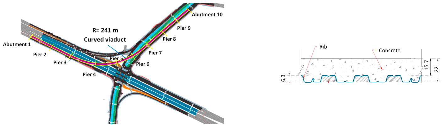
To the north of Morelia, a highway interchange has been built to connect the city with Salamanca via the Morelia–Salamanca highway (MEX 43). The interchange is located at latitude 19.721802° and longitude 101.188397°. Figure 1 shows the curved bridge that is the focus of this study.
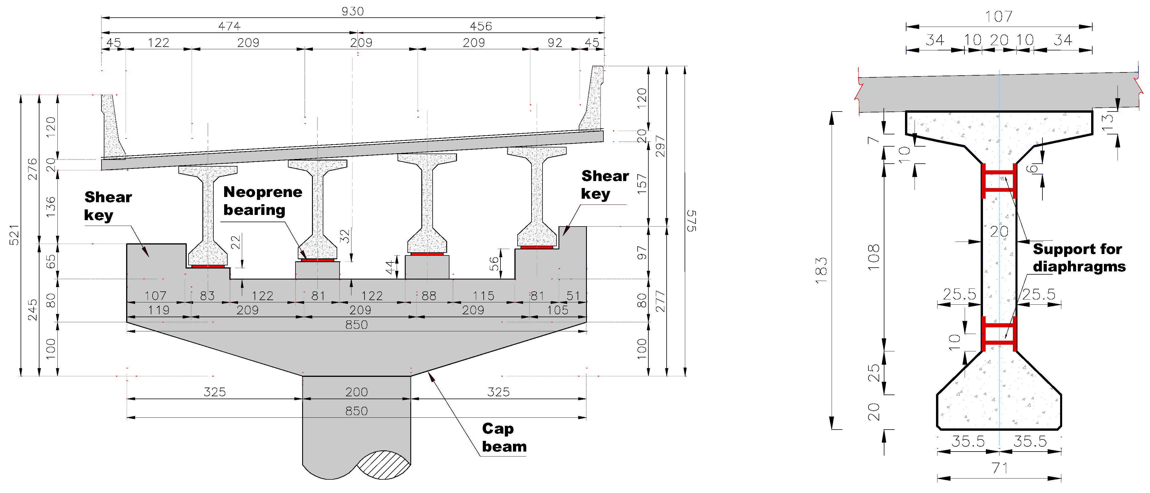
The bridge consists of nine simply supported spans of varying lengths, totaling 367 m. Figure 2 shows a drawing of the viaduct’s geometry (in yellow) with a radius of curvature (R) of 241 m. The reinforced-concrete deck slab, constructed with a steel orthotropic deck, has a total thickness of 0.22 m. Figure 3 shows an elevation in pier 2 and the cross-section of the AASHTO Type VI beams. The viaduct accommodates two traffic lanes, with a total width of 9.30 m. Each span features six steel diaphragms that connect the AASHTO girders transversely.
The AASHTO beams rest on neoprene supports with plan dimensions of 0.60 × 0.40 m and thicknesses of 0.057 m at one end and 0.073 m at the other. The design compressive strength of the reinforced concrete in the deck slab was f’c = 29.42 MPa, while f’c = 49.03 MPa in AASHTO girders. The reinforcing steel had a tensile strength of fy = 414 MPa.

2.2. Substructure

Pier bent abutments 1 and 10 are located at the entrance and exit of the curved viaduct. Each abutment includes a rectangular bent cap measuring 1.8 m wide by 1.5 m deep, supported by two circular reinforced-concrete columns with a 1.5 m diameter. Abutment 1 has a height of 4.71 m, while abutment 10 has a height of 2.82 m.
The piers consist of reinforced-concrete single columns with a 2.0 m diameter and heights ranging from 6.20 to 18.40 m (see Table 1). The table also lists the longitudinal steel reinforcement (As) for the columns. The piers’ hammerhead has a width of 2.70 m and a variable depth ranging from 0.80 to 1.80 m. The design compressive strength of the reinforced concrete used in the piers, caps, and shear keys is 29.42 MPa.

3. Ambient Vibration Measurements

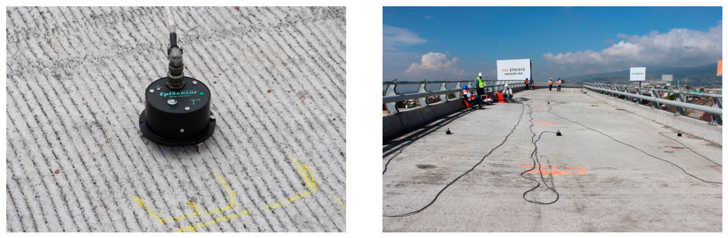
The viaduct’s dynamic properties were determined experimentally through a campaign of ambient vibration measurements conducted before its inauguration. Three Kinemetrics EpiSensor FBA ES-T triaxial sensors were used, each with a full-scale recording range of ±0.25 to ±4g. These sensors, which integrate three force-balance accelerometers in a single unit, were connected to a Granite-12 acquisition console capable of supporting up to 36 channels.
Measurements were conducted before the asphalt layer was placed on the bridge (Figure 4). Initially, a measurement campaign was conducted on the deck between piers 5 and 6, with five measurements, each lasting 10 min. In the first measurement (M1), a fixed triaxial sensor was positioned at the center of the span and remained there throughout all five measurements. Additionally, three triaxial sensors were placed at the end of the slab near pier 6. The second measurement (M2) was taken after relocating the three sensors to a position one-quarter of the way across the span near pier 6. For the following measurement (M3), the sensors were moved to the center of the span. The fourth and fifth measurements (M4 and M5) were conducted with the sensors positioned three-quarters of the way across the span (measured from pier 6) and at the deck end near pier 5, respectively.
In the second measurement campaign, measurement 6 involved keeping the fixed sensor at the center of the span between piers 5 and 6. The three triaxial sensors were then relocated to the centers of the spans between piers 2–3, 3–4, and 4–5 for measurement M6.
For measurement M7, the three triaxial sensors were placed at the centers of the spans between piers 6 and 7, 7 and 8, and 8 and 9. In the subsequent measurement (M8), one triaxial sensor was positioned halfway across the bridge’s width between piers 6 and 7, near pier 6; the second sensor was placed between piers 7 and 8, near pier 7; and the third sensor was located between piers 8 and 9, near pier 8.
Finally, in the last measurement (M9), a triaxial sensor was positioned midway across the bridge’s width between piers 2 and 3, near pier 3. The second sensor was placed between piers 3 and 4, near pier 4, and the third sensor was located between piers 4 and 5, near pier 5.
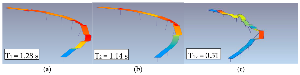
The recorded signals were analyzed using the ARTeMIS V4.0 software [42] with the Operational Modal Analysis and Enhanced Frequency Domain Decomposition Technique (EFDD). The first frequencies were estimated from the singular values of the spectral densities. Figure 5 illustrates three vibration modes identified in the analyses. The first three experimentally identified modes correspond to two transverse modes (f1 = 0.781 Hz, f2 = 0.879 Hz) and the deck’s fundamental vertical bending mode (f3 = 1.961 Hz). The damping ratios identified via the Enhanced Frequency Domain Decomposition (EFDD) technique for these operational modes ranged between 1.1% and 1.8%. These low damping values reflect the linear elastic state of the uncracked bridge components subjected exclusively to micro-strain excitation levels during ambient testing. The experimental campaign reliably identified the three dominant global modes but did not provide sufficient signal-to-noise resolution to independently calibrate all higher-order transverse and torsional modes. These modes are nevertheless retained in the three-dimensional numerical model. Since all the spans are simply supported at both ends, several modal shapes correspond to the bridge’s transverse motion. The primary modes exhibiting lateral movement in two sections of the viaduct are illustrated. In the first case, the slabs mainly displace laterally between piers 3–7; in the second, the modal shape reflects transverse movement between piers 5–7. In these three modes, the off-diagonal terms of the MAC matrix are less than 0.20. The estimate was also validated using modal complexity percentages of 10%, 2%, and 18% for the three modes, respectively.

4. Material and Methods

4.1. Elastic Model

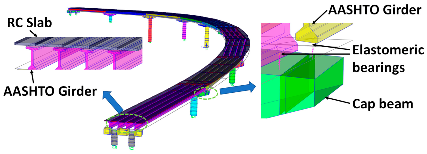
A numerical model of the viaduct was created using SAP2000 V24.0 [43] and calibrated with ambient vibration measurements. Bar elements with six degrees of freedom at each node represented the beams, columns, headers, and diaphragms. The slab was modeled using Shell-Thin elements, which provide six degrees of freedom at each node. The elastomeric bearings were represented with link elements. Additionally, the piers’ columns were divided into several segments (1.6–2.0 m long) to distribute each column’s mass along its length. The bridge model assumed a critical damping ratio of 5%. The studies mentioned in the introduction, along with many others, employed structural elements with the same characteristics and degrees of freedom used in this study. The compressive strength of the concrete used for the columns and bent caps was 29.42 MPa, whereas that of the AASHTO Type VI girders was 49.03 MPa. The elastic modulus was calculated using the expression E = 14,000 f c , resulting in an elastic modulus of E = 23.78 GPa for columns and bent caps, and E = 30.70 GPa for AASHTO girders.
The elastomeric bearings have dimensions of 0.60 m × 0.40 m, Shore hardness of 60, shear modulus G = 1 MPa, bulk modulus k = 2000 MPa, shape factor S = 9.2, tensile strength of 17.2 MPa, and an ultimate elongation of 350%. The 0.057 m thick bearing consisted of three interior rubber layers, each 0.013 m thick; two rubber covers, each 0.003 m thick, and four steel shims, each 0.003 m thick. The 0.073 m-thick bearing consists of four interior rubber layers, each 0.013 m thick, two rubber covers, each 0.003 m thick, and five steel shims, each 0.003 m thick. The horizontal stiffness of the supports is 5230 kN/m at t = 0.057 m and 4058 kN/m at t = 0.073 m. The vertical stiffness is 87,303 kN/m at t = 0.057 m and 67,735 kN/m at t = 0.073 m. The expansion joints were modeled using gap-type link elements that exhibit nonlinear behavior. Figure 6 shows the numerical model developed in SAP2000 V24.0.
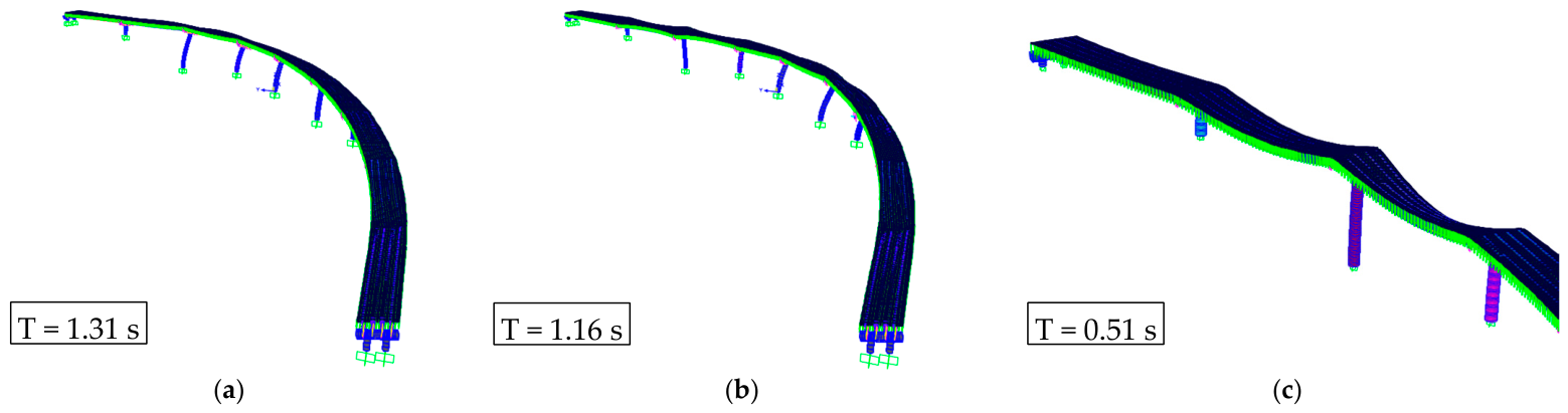
Initially, the viaduct’s vibration modes were determined without accounting for the asphalt layer’s mass, reflecting the bridge’s condition during environmental vibration measurements. In this scenario, the bridge’s mass comprised the self-weight of all structural components, including piers, abutments, heads, girders, and slabs, as well as non-structural elements such as parapets, kerbs, and rails. Figure 7 displays the mode shapes and periods for the first two transverse vibration modes, as well as the first bending mode of the deck slab. The calibration involved an 8% increase in the initial concrete modulus of elasticity to represent the dynamic uncracked stiffness under ambient excitation, along with removal of the asphalt-overlay mass because the overlay was absent during the ambient-vibration campaign.
Table 2 compares experimentally identified and computed dynamic properties. The correlation between experimental and numerical mode shapes was satisfactory, with the maximum frequency error below 2.3% and Modal Assurance Criterion (MAC) values above 0.88.
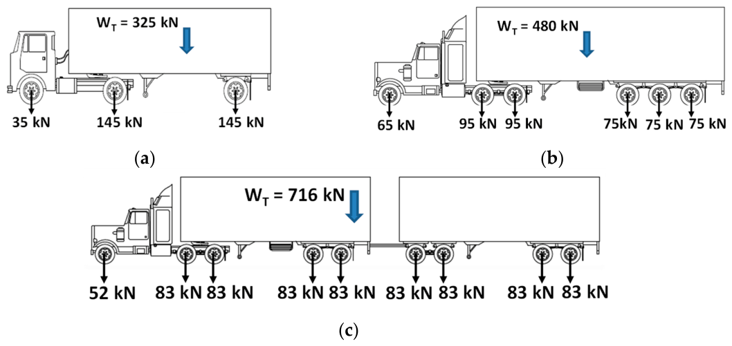
Adding the asphalt layer increases the periods in the transverse and vertical directions to 1.40 s, 1.24 s, and 0.55 s, respectively. For the bridge design, the live load was based on the most unfavorable traffic combination: one lane with an HS-20 vehicle and the other with a T3-S3 vehicle or an HS-20 combined with a T3-S2-R4 truck. Figure 8 shows the design trucks, detailing the load on each axle and the vehicles’ total weight (WT).

4.2. Nonlinear Model

The bridge’s nonlinear analysis was performed using a numerical model created in PERFORM 3D software V8.0 [44]. A concentrated plasticity model was used for the columns, with plastic hinges assigned at both ends of the elements (abutments and piers). The columns were discretized into one-meter-long elements to account for the distributed mass of the piers. Mander et al. [45] developed a constitutive model to characterize the uniaxial stress–strain behavior of confined and unconfined concrete. The stress–strain relationship for reinforcing steel followed the model proposed by Park and Paulay [46]. The analysis assumed elastic behavior for reinforced concrete slabs, AASHTO beams, pier caps, and diaphragms. The deck was modeled using a 4-node quadrilateral shell element with 6 DOFs per node. AASHTO girders, pier caps, and diaphragms were modeled with elastic beam elements with 6 DOFs per node. Although the ambient vibration test yielded low operational damping ratios (1.1–1.8%), a viscous damping ratio of ζ = 5 % was selected for linear dynamic response spectrum and baseline non-linear dynamic analyses. This assumption aligns with standard seismic bridge provisions [47,48] to represent high-amplitude energy dissipation mechanisms, such as micro-cracking and friction at expansion joints/bearings, that are activated during earthquake shaking.
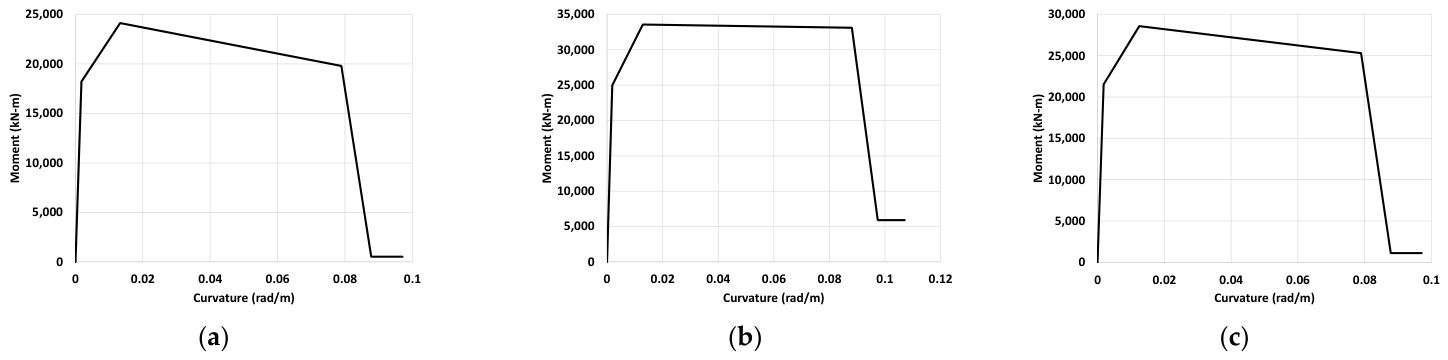
Figure 9 displays the backbone curves derived from the moment–curvature diagrams, which describe the nonlinear behavior of column plastic hinges. PERFORM 3D V8.0 defines the hysteretic behavior of the elements based on these curves using straight lines that mark (from left to right) the yield strength (Y), ultimate strength (U), ductile limit(L), residual strength(R), and failure point(X). Table 3 presents the bending moment and curvature for each point, calculated from the moment–curvature analysis of the substructure elements.
Additionally, the software employs Clough’s rule [49] to describe the stiffness degradation. The parameters adopted in this study were Y = 0.90, U = 0.70, L = 0.50, R = 0.35, and X = 0.35, based on Jara et al. [50], which selected these values from experimental results of concrete columns subjected to cyclic loading.
The bridge has 0.05 m-wide expansion joints between each simply supported span. These joints were modeled using gap elements that add stiffness only after the joint closes. The modeling approach proposed by [51] was used to represent the elastomeric supports. The model is elastoplastic and begins with a shear stiffness defined as K = GA/hr, where G is the shear modulus, A is the bearing area, and hr is the total thickness of the neoprene. The linear elastic behavior ends when the sliding force, denoted by Fd = Nμ, is reached. Here, N is the normal force acting on the bearing, and μ = 0.4 [15,48] is the coefficient of friction between the girder’s concrete and the elastomeric bearing.
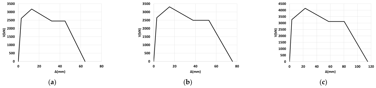
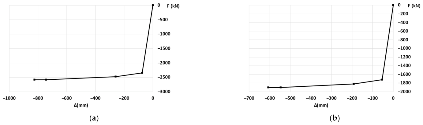
Shear keys on the pier caps provide lateral support to the exterior girders. The numerical model for the shear keys was adapted from Megally et al. [52]. Figure 10 shows the shear–displacement (V-Δ) relationships for shear keys on piers 2, 5, and 8. The capacity of the shear keys varies with their geometry, which differs from pier to pier.
The embankment approach was modeled using nonlinear translational spring elements with a four-linear behavior that accounts for the soil’s passive action [53]. Figure 11 shows the passive action behavior of abutments 1 and 10.

5. Seismic Demand

Interplate, intraplate, and crustal seismic sources contribute to Morelia’s seismic hazard. The interplate source along Mexico’s Pacific coast causes most seismic activity and can produce earthquakes up to magnitude 8.4. Intraplate earthquakes occur at intermediate depths within the oceanic plate, which is already subducted beneath the continental plate, and can reach magnitudes as high as 8.1. These earthquakes have epicenters near inland cities. Additionally, a crustal seismic source [54,55] generates shallow earthquakes along the Trans-Mexican Volcanic Belt, capable of producing maximum magnitudes of up to M = 7.6.
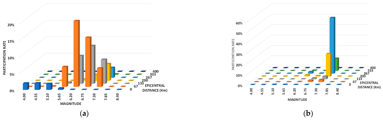
A recent seismic hazard assessment for Morelia determined uniform seismic hazard spectra for firm soils [56]. To evaluate site effects, we analyzed data from geotechnical studies and accelerograms recorded in Morelia by the Nicolaita Seismic Network, which comprises eleven accelerographs. Figure 12 shows the disaggregation of seismic hazard for Peak Ground Acceleration (PGA) and for the spectral period of 1.40 s, corresponding to the bridge’s first transverse mode. The interplate seismic source, situated more than 200 km from Morelia, is the most active fault. Intraplate earthquakes can occur more than 65 km from the city, and two local seismic sources (crustal earthquakes) could produce events with magnitudes up to 6.4 (M = 6.4). According to the site-specific hazard disaggregation (Figure 12), crustal and intraplate seismic sources contribute significantly to Peak Ground Acceleration (PGA) in Morelia. However, at the fundamental transverse period of the viaduct (T1 = 1.40 s), the seismic hazard is governed almost exclusively by interplate and intermediate-depth intraplate sources, while the participation of local crustal events becomes negligible. Because shallow crustal earthquakes generate ground motions dominated by high frequencies (short periods), they produce low dynamic amplification in intermediate-to-long-period flexible structures. Consequently, we excluded crustal records from the non-linear dynamic analyses, allowing the study to focus on the two independent seismic sources that impose critical demand on the bridge.
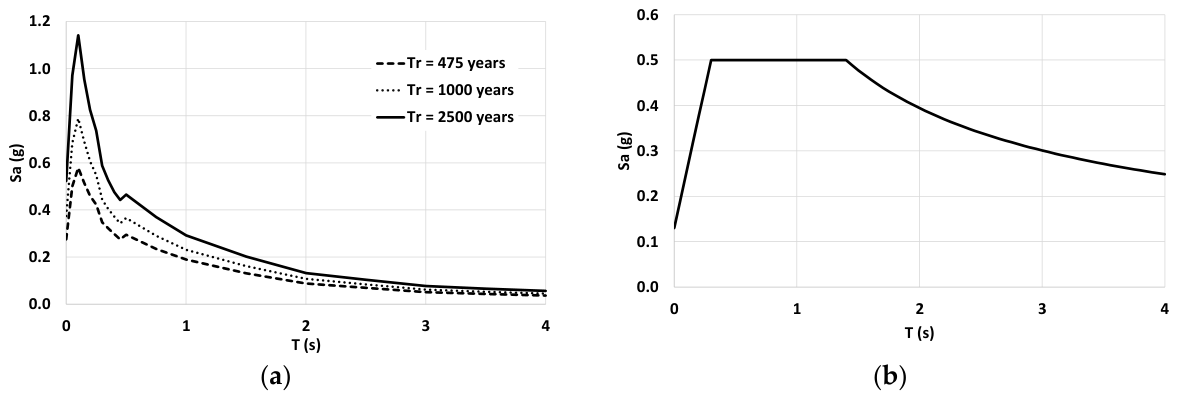
The seismic station of the Nicolaita Seismic Network at the Faculty of Psychology is 250 m from the bridge. Based on the seismic hazard assessment for firm soil, analysis of accelerograms recorded at this station, and a geotechnical study of the site, uniform seismic hazard spectra were derived for different return periods (Tr). Figure 13 displays the uniform hazard spectra and the design spectrum used for the viaduct’s structural design. Notably, the design spectrum plateau is close to the maximum amplitude of the uniform hazard spectrum (UHS) for a return period of 475 years.
A set of accelerograms was collected from the UNAM accelerographic records database to evaluate the viaduct’s seismic vulnerability [57]. To ensure that the selected ground motions adequately represent the seismic hazard at the bridge site, the accelerograms were selected based on specific criteria derived from local hazard disaggregation, geotechnical characteristics, and accelerograms recorded near the Viaduct. According to the seismic hazard assessment for Morelia, interplate and intraplate sources contribute the most. 46 interplate seismic records were selected based on earthquakes that occurred along the Mexican Pacific subduction zone with magnitudes M ≥ 6.0 and recorded at epicentral distances of 220 to 275 km (the distance from Morelia to the interplate earthquakes). For the intraplate fault, 32 intermediate-depth earthquakes within the subducting plate were selected with magnitudes M ≥ 6.0 and epicentral distances ranging from 84 to 243 km. The minimum magnitude was set to reduce the scale factors applied to seismic records for different return periods. The selected populations also preserve the characteristic duration and frequency content associated with interplate and intraplate earthquakes.
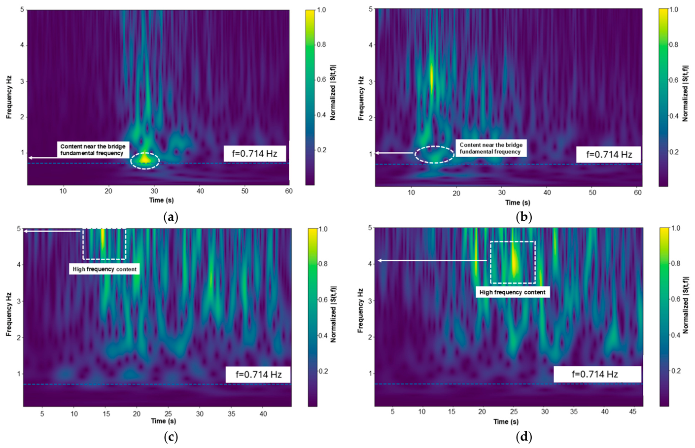
To further characterize the time–frequency content of the ground motions, a Stockwell Transform (S-transform) analysis was performed for eight interplate and intraplate records. The analysis focused on the frequency range from 0.1 to 5 Hz and considered the viaduct’s fundamental frequency, f1 = 0.714 Hz (T1 = 1.40 s). Representative results (Figure 14) show distinct time–frequency characteristics between the two ground-motion populations. The S-transform was evaluated over the frequency range from 0.1 to 5.0 Hz using the original sampling intervals of the records. We linearly detrended the signals before analysis and excluded the first and last 2 s of each record when calculating the quantitative frequency and energy measures to reduce edge effects.
The analysis revealed clear differences in the time–frequency characteristics of the two ground-motion populations. The average frequency corresponding to the maximum time-averaged S-transform power was approximately 1.79 Hz for the interplate records and 3.81 Hz for the intraplate records. More importantly, the interplate records exhibited a substantially higher proportion of energy in the frequency range relevant to the fundamental mode. Using the same 0.1–5.0 Hz frequency range for all records, the mean fraction of S-transform energy in the 0.50–1.00 Hz band was approximately 9.8% for the interplate records, compared with 2.9% for the intraplate records. In the narrower 0.60–0.85 Hz band around f1 = 0.714 Hz, the corresponding values were approximately 5.4% and 1.5%, respectively.
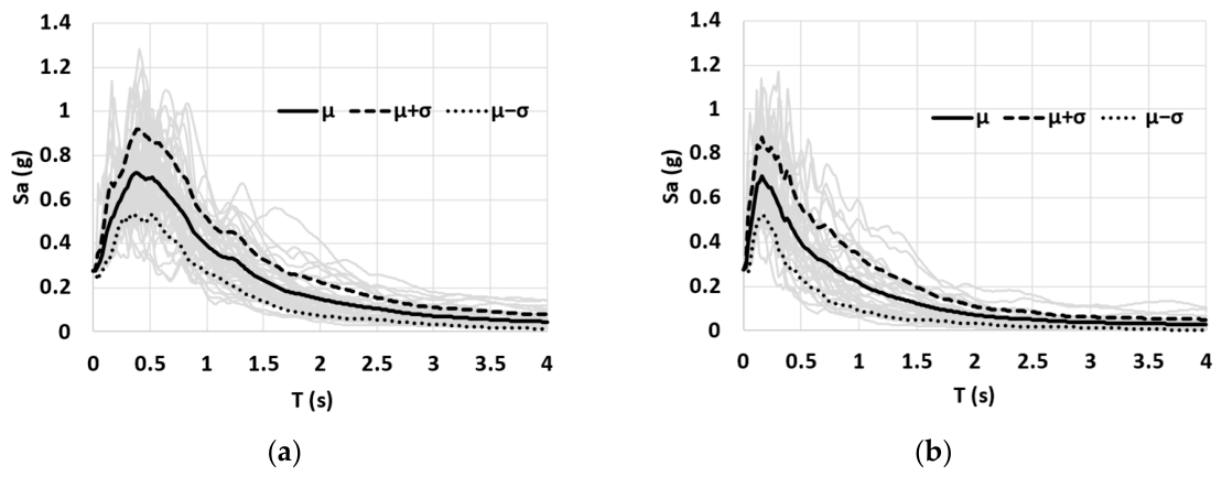
Regarding site conditions, the response spectra of the selected seismic records followed the shape of response spectra from existing accelerograms recorded near the Viaduct (approximately 250 m). In addition, the medium response spectrum of the selected seismic records (Figure 15) matches the shape of the uniform response spectrum for the bridge’s specific location (Figure 13a). The selected sets inherently capture the physical duration and frequency content characteristic of subduction (interplate) and in-slab (intraplate) events in Mexico. Interplate records exhibit longer durations and rich spectral content in the medium-to-long period range, whereas intraplate records show higher energy at shorter periods.
The seismic records were scaled to different return periods of the uniform hazard spectra based on Peak Ground Acceleration (PGA). PGA was adopted as the common scaling parameter because the site-specific seismic hazard characterization used in the study was expressed in terms of PGA, and because a common PGA-based intensity measure allowed the two ground-motion populations to be compared consistently at the investigated return periods while preserving their source-dependent spectral characteristics. Scaling by PGA does not imply that PGA alone governs the bridge response. At the 475-year intensity level, both record populations were scaled to the same PGA of approximately 0.27 g, but the mean spectral acceleration at (T1 = 1.40) s was approximately 0.33 g for the interplate records and 0.19 g for the intraplate records (Figure 15). Thus, the two ground-motion populations preserved different spectral characteristics. Previous studies have also used PGA as an intensity measure for probabilistic seismic demand analyses of structures [58,59,60,61,62].
The scaling factor was calculated by dividing the expected peak ground acceleration from the uniform hazard spectrum (0.27 g for Tr = 475 years) by the maximum peak ground acceleration across the horizontal components. This factor was then used to scale the seismic records for both horizontal components. The initial amplitude scaling corresponded to a 475-year return period, which is commonly used in seismic design regulations. Figure 15 shows the response spectra of the geometric mean of the two horizontal components of the seismic records, scaled to a 475-year return period. It also shows the mean (μ) and the mean ± one standard deviation (μ ± σ) of the response spectra for the two seismic sources.
The viaduct is expected to experience high seismic intensities from interplate events. This seismic source, characterized by larger epicentral distances, produces high amplitudes in the medium- to long-period spectral zone.

6. Nonlinear Analysis

6.1. Return Period Tr = 475 Years

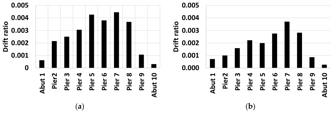
The numerical model for the nonlinear analysis of the viaduct, created with Perform3D program V8.0 [44], was subjected to two horizontal components of the set of accelerograms scaled to PGA of 0.27 g, corresponding to a return period of Tr = 475 years. The average maximum drift ratios (averaged across the seismic demands in the viaduct for each group of accelerograms) indicated that all piers remained within the elastic range for this 475-year return period. Figure 16 shows the bridge’s average drift ratios under seismic records from interplate (Figure 16a) and intraplate (Figure 16b) sources.
The differences in the dominant periods of seismic motion between the two sources led to higher drift-ratio demands on the viaduct during interplate events than during intraplate earthquakes. For interplate earthquakes, the highest drift ratios were observed at piers 5 and 7, with values of 0.0042 and 0.0044, respectively. For intraplate seismic records, the highest drift ratios were observed at piers 7 and 8, with values of 0.0037 and 0.0028, respectively. These results can be attributed to the length of piers 5–8, which are the tallest columns in the viaduct.
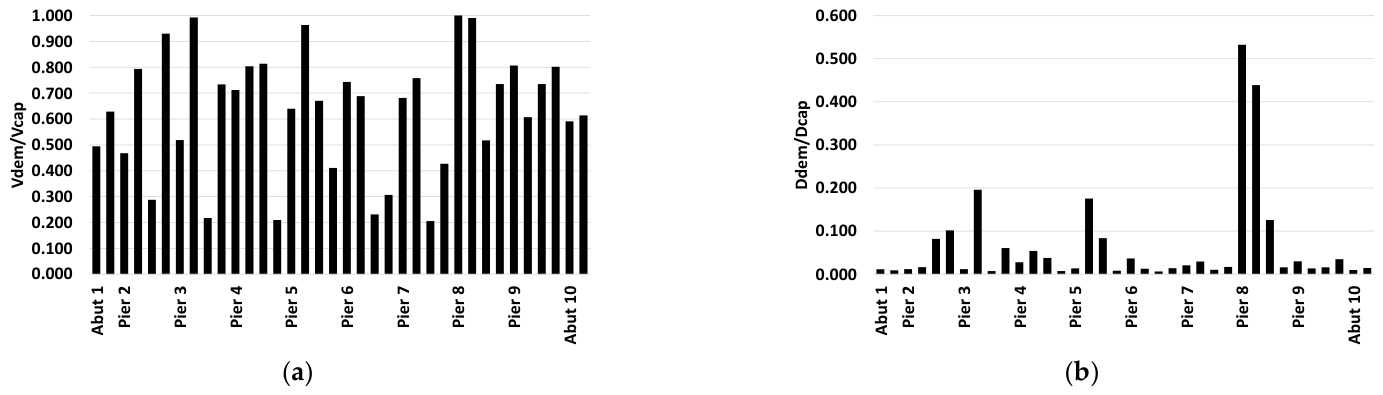
Figure 17 shows the shear force demand/capacity ratio (Vdem/Vcap) and the displacement demand/capacity ratio (Ddem/Dcap) for each shear key. The demands shown represent the ensemble mean across the ground-motion suite for each shear key, preserving spatial differences across the bridge width. The figure shows two bars for the abutments (one shear key at each bent cap end) and four bars for each pier (two outer-curve and two inner-curve shear keys). The results clearly highlight the torsional asymmetry of the curved deck: shear keys on the outer curve experience significantly greater displacement demands than those on the inner curve. Figure 17a presents the ratios of shear force demand to capacity, while Figure 17b displays the displacement ratios.
The shear keys on piers 2, 3, 5, and 8 are nearly at their maximum strength. However, none of them have reached their displacement capacity. This indicates that while this seismic intensity level could damage the shear keys, they would not fail or collapse.
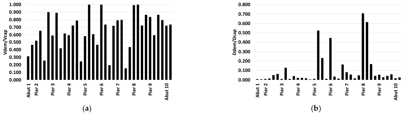
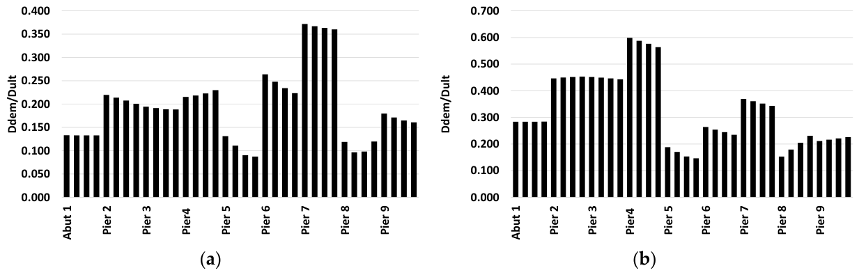
Figure 18 displays the seismic response of the shear keys when the bridge was subjected to the set of seismic records from the interplate source. Once again, the number of bars in the figure for each substructure element corresponds to the number of shear keys in each abutment and pier. Figure 18a presents the ratios of shear force demand to capacity, while Figure 18b displays the displacement ratios.
The shear force demands of interplate earthquakes were slightly higher than those from seismic records of the intraplate source, reflecting the higher spectral intensities of interplate seismic records at the bridge’s fundamental period. The displacement demands increased significantly, especially at the shear keys of piers 5, 6, and 8, the bridge’s tallest piers. However, none of the shear keys reached their ultimate displacement capacity.
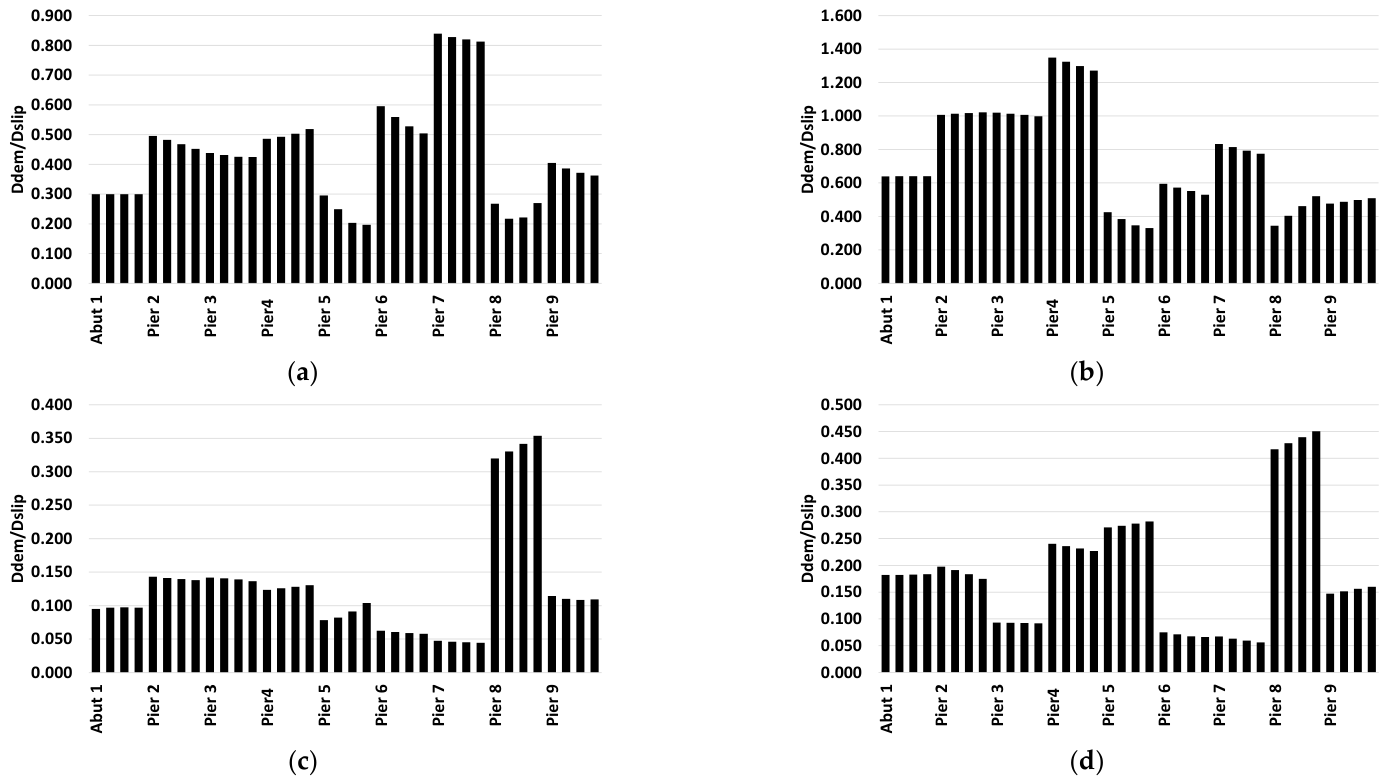
Figure 19 shows the ratio of displacement demands to the sliding-capacity displacement for the 57 mm thick neoprene bearings. The figure includes two graphs showing the bridge’s average longitudinal response: one for intraplate sources (Figure 19a) and another for interplate sources (Figure 19b). Additionally, two graphs present the same ratios for the average transverse response (Figure 19c,d).
A ratio below one indicates that the displacement demand did not exceed the displacement required to cause the support to slide on the concrete beam cap. When the bridge was subjected to the set of accelerograms from the interplate seismic source, the bearings on piers 2, 3, and 4 reached the longitudinal sliding displacement; however, the demands remained moderate. The displacement demands on the 73 mm-thick bearings were lower than those on the 57 mm thick bearings and did not exceed the sliding displacement. Slightly shorter periods in the longitudinal direction than in the transverse direction increase seismic demands (See Figure 15).
According to Magsoudi-Barmi et al. [63], bearing failure occurs at a distortion level of 250%. Figure 20 illustrates the ratio of average longitudinal displacement demands for the 57 mm thick bearings, normalized by their ultimate-capacity displacement. When the bridge was subjected to a set of seismic records from the interplate source, the maximum demand reached 60% of the ultimate bearing capacity at pier 4. In contrast, the displacement demands on the bearings of the other piers were significantly lower. Intraplate seismic records showed a maximum demand of about 35% of the bearing capacity at pier 7, with lower demands on the remaining bearings.
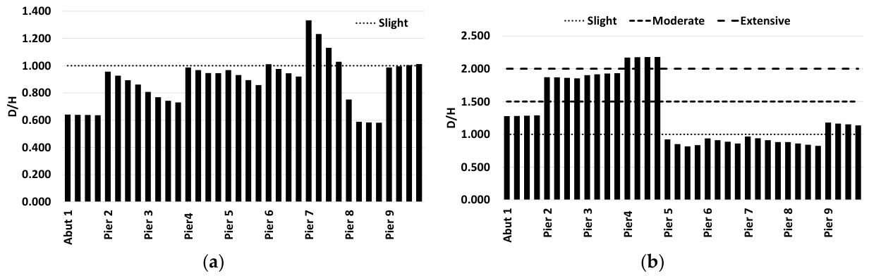
To assess the expected damage to bridge bearings from the 475-year earthquake, Figure 21 presents the D/H ratios for the 57 mm thick bearings in the bridge’s longitudinal direction. D is the horizontal average displacement demand, while H denotes the total thickness. The figure also includes the damage limit states proposed by Maghsoudi–Barmi et al. [63]. The D/H ratios of 1.0, 1.5, 2.0, and 2.5 correspond to slight, moderate, extensive, and collapse damage, respectively.
When the bridge was subjected to interplate seismic records, the longitudinal displacement demands in the bearings on piers 3, 4, and 5 were estimated to fall between the slight and moderate damage limit states. No damage is expected in the other bearings. In summary, for the design earthquake (Tr = 475 years), the viaduct is expected to experience minor damage.

6.2. Return Period Tr = 2500 Years

Both sets of accelerograms from the two seismic sources were later scaled for an extraordinary earthquake, assuming a 2500-year return period. Figure 22 shows that the displacement demands in the piers have increased significantly compared to those for the 475-year earthquake. The figure also displays the expected damage limit states according to Hazus 5.1 [64].
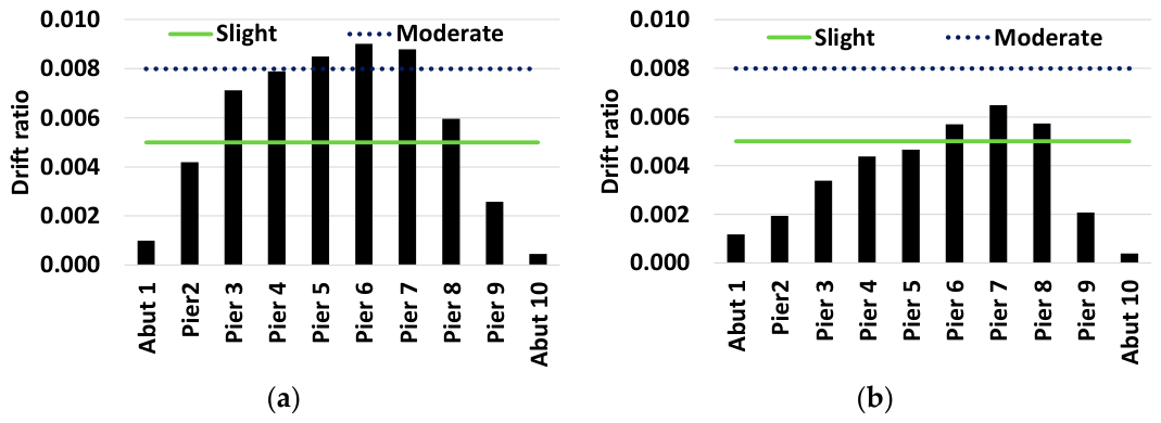
The maximum drift-ratio demands occur when the bridge is subjected to seismic records from the interplate seismic source (Figure 22a). According to Hazus 5.1 [64], piers 5–7 would be in the moderate-to-extensive damage range (0.008–0.020); piers 3, 4, and 8 would experience slight-to-moderate damage; and the other piers and abutments would remain below the slight-damage limit. The maximum seismic demands on the piers from intraplate earthquakes (Figure 22b) placed piers 6–8 in the slight-to-moderate damage state. In contrast, all other piers and abutments have drift-ratio demands below the slight-damage limit state.
Figure 23 shows the shear force demands in the shear keys normalized by the capacity of these elements (Vdem/Vcap) and the displacement ratio demands (Ddem/Dcap) when the bridge was subjected to the set of accelerograms from the intraplate seismic source. The shear keys on piers 3, 5, and 8 reached their maximum strength, while those on piers 4, 6, and 9 exceeded 90% of their capacity.
The displacement demands on the shear keys do not exceed their maximum capacity at any pier. The highest demand occurs at pier 8 (the tallest column), where the shear keys on the bridge’s outer curve reach 62% and 75% of their capacity. Piers 3 and 5 follow, with displacements of 42% and 60% of their maximum capacity, respectively.
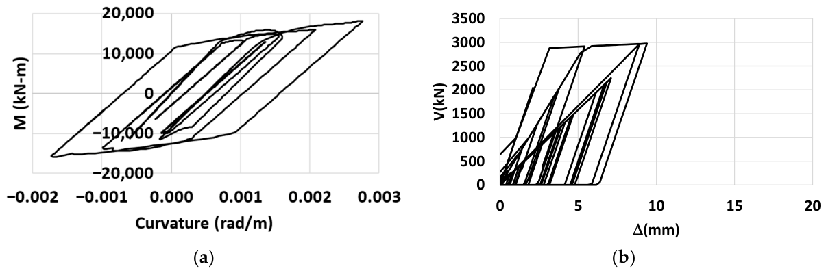
Figure 24 shows, as an example of hysteretic loops in columns and shear keys, the seismic response of Pier 5 and one shear key on the cap beam of this pier under a seismic record from an interplate source, scaled for a 2500-year return period.
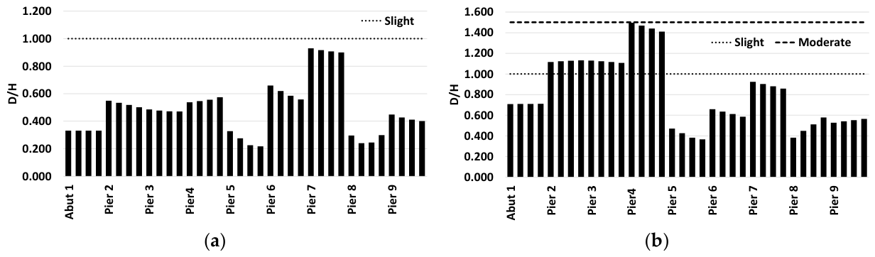
To evaluate the expected damage to the elastomeric bearings, Figure 25 shows the D/H ratios along the bridge’s longitudinal direction. The displacement demands derived from the accelerograms of the intraplate source (Figure 25a) indicated that the maximum D/H values placed the bearings on pier 7 between the thresholds for slight and moderate damage. In contrast, all other bearings fell below the threshold for slight damage.
When analyzing the bridge using the set of accelerograms from the interplate seismic source (Figure 25b), the bearings on piers 5 to 8 showed no damage. However, the bearings at abutment 1 and pier 9 experienced slight to moderate damage. The bearings on piers 2 and 3 showed damage ranging from moderate to extensive, while those on pier 4 exceeded the threshold for extensive damage.

6.3. Reliability Index

The previous results provided insights into the bridge’s expected behavior for two return periods. However, seismic regulations set seismic design parameters by limiting the probability of failure, which is measured indirectly through a reliability index. To assess the reliability index, the accelerograms from the interplate seismic source were scaled up to the point of bridge failure. The bridge collapse was presented using seismic records of the 2500-year earthquake, scaled by a factor of 1.80. The reliability index reported in this study applies specifically to this pier-failure-based collapse limit state and should not be interpreted as a comprehensive system reliability index that accounts for all possible interactions among components and failure modes. The incremental scaling procedure adopted herein follows the basic concept of Incremental Dynamic Analysis (IDA), where each record is independently subjected to progressively increasing intensity levels. However, this analysis focused on identifying the onset of the defined collapse limit state, rather than developing probabilistic fragility functions for multiple damage states [65]. The scaling began at the PGA level corresponding to a 2500-year return period. At each stage, we increased the ground-motion amplitudes incrementally by 20% and assessed the bridge demands. This process continued until pier failure was observed; the resulting collapse distribution followed a lognormal probability density function, with a median equal to the scaled PGA required to reach failure.
The incremental scaling to collapse was performed solely with the interplate ground-motion suite, as these records determine the dominant structural demands across all intensity levels. The spectral content of these ground motions is rich near the fundamental period (T1 = 1.40 s). Conversely, intraplate records are dominated by short-period energy (T ≈ 0.26 s) and would require larger PGA scaling factors to reach collapse. However, the reliability index subsequently obtained must be interpreted specifically as the reliability estimate associated with the defined collapse limit state and the adopted intraplate ground-motion population, rather than as a universal reliability index for both seismic-source classes.
The record-specific scale factors required to reach the collapse intensity were large because the interplate records were recorded at epicentral distances of approximately 220–275 km, representing the actual distance from the study site to the subduction interplate source. The scale factors used in the incremental procedure ranged from approximately 7 to 34. This high-amplitude scaling serves as a numerical mechanism to force structural failure and does not represent a physical hazard scenario for a specific return period.
Across all evaluated ground motion records, damage consistently initiated at the exterior shear keys because of the deck’s transverse–torsional coupling. Subsequent damage progression, marked by shear concentration in shorter piers and abutments, followed a stable, geometrically driven pattern. Consequently, the reported mean values accurately capture the bridge system’s critical failure mechanism and governing limit states.
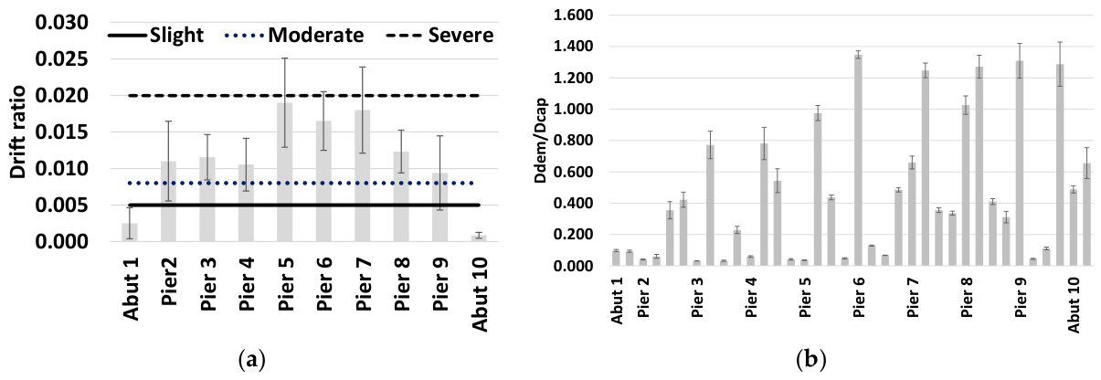
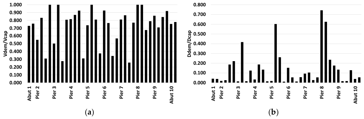
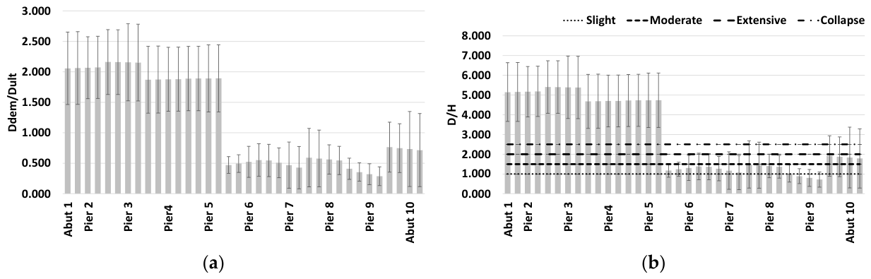
Figure 26a shows the drift-ratio demands for the bridge piers, which fell within the moderate-to-severe damage limit states. In contrast, the abutments exhibited drift-ratio demands below the threshold for slight damage. Piers 5, 6, and 7 experienced the highest seismic demands.
Figure 26b shows the displacement-ratio demands for the shear keys at this seismic intensity level. Six shear keys (on piers 6 to 9) have now exceeded their displacement capacity (Ddem/Dcap > 1), and one more (pier 5) is very close to reaching this value. In nearly all cases, failure would occur at the shear keys on the bridge’s outer curve.
Figure 27 presents the longitudinal seismic demands on the 57 mm thick bearings subjected to interplate accelerograms. Figure 27a shows the bearings’ displacement-to-capacity ratios, and Figure 27b displays the D/H ratios, which include the expected damage limit state. The bearings on abutment 1 and piers 2, 3, and 4 exhibited demands exceeding the collapse limit state (D/H = 2.5). Conversely, the supports on piers 5 to 8 showed demands below the moderate-damage limit state.
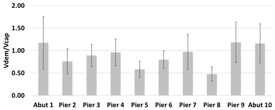
The pier drift ratios led to damage ranging from moderate to severe. Additionally, shear failures are commonly observed in bridges subjected to seismic actions. Therefore, we evaluated the shear force demand-to-capacity ratios for the bridge piers. The shear capacity of the viaduct columns was determined in accordance with the most recent Mexican regulations for concrete structure design [66]. Table 4 presents the analysis used to determine the shear capacity of the columns. Ag is the gross area; As is the area of longitudinal reinforcement; Pu is the ultimate axial load for each column; Vc is the shear strength provided by concrete; vs. is the shear strength provided by transverse reinforcement (No. 4 hoops @ 0.20 m); Vc is the shear capacity; and Vd is the shear demand.
Figure 28 shows the shear demand-to-capacity ratios (Vdem/Vcap) for the piers and abutments. Abutments 1 and 10, along with the shortest pier (pier 9), exceeded their maximum shear capacity, resulting in failure. Additionally, piers 4 and 7 exhibited shear demands very close to their maximum capacity.
Record-to-record variability was quantified by reporting the mean demand and ± one standard deviation for each structural component. The revised results indicate that dispersion is response- and component-dependent, with most coefficients of variation ranging from 0.25 to 0.50. The largest relative dispersion occurs across several component-level force and displacement demands, whereas substructure drift shows comparatively less variability. This dispersion indicates that individual ground motions may produce demands substantially different from the mean response. Consequently, the sequence of component limit-state exceedance cannot be inferred solely from the mean demands; the mean response identifies the general critical components, while the standard deviation characterizes the range of responses across the different ground motions.
In summary, the expected behavior of the viaduct under the seismic records from the interplate source indicates that both the abutments and pier 9 would likely experience shear failure. Additionally, seven shear keys reached their displacement capacity in the bridge’s outer curve zone. Moreover, 16 elastomeric bearings exceeded their collapse limit. The damage process begins with shear key failure, particularly on piers 6–9. Subsequently, shear failure occurs in the abutments and in piers 7 and 9 in the bridge’s transverse direction. It is assumed that this seismic intensity level caused the bridge’s failure, and it was used to assess its reliability index.
The reliability index in the useful life of the bridge ( T ), is defined with Equation (1).
β f = Φ 1 ( P f , T )
β f is the reliability index, Φ 1 is the inverse cumulative normal function and P f , T is the failure probability in the useful life ( T ), defined with Equation (2). In this case, the PGA mean value of the probability distribution P f , T , was assumed to be the PGA intensity for the final scaling in the previous analyses.
P f , T = 1 e λ f T
Equation (3) assumes that earthquake occurrences follow a Poisson Process, where λ f is the annual failure rate for the damage limit state under analysis.
λ f = i m P f | i m d λ i m
P f | i m is the probability of reaching the failure limit state, given a seismic intensity ( i m ). λ i m is the exceedance rate of the seismic intensity at the site and d λ i m is the negative derivative of λ i m with respect to the seismic intensity.
The conditional probability of failure P f i m is formulated by assuming lognormal distributions for both structural capacity ( C ) and seismic demand ( D ). For a given intensity measure ( i m ), the median seismic demand ( D ) is obtained from the nonlinear dynamic analyses, while ( C ) represents the median capacity associated with the defined collapse limit state (Equation 4). The conditional probability is therefore calculated as:
P f i m = Φ l n D l n C β D 2 + β C 2
where β D and β C are the logarithmic dispersions of demand and capacity, respectively. The resulting conditional fragility is then combined with the annual exceedance-rate curve of the seismic intensity through the standard convolution procedure to obtain the annual failure rate.
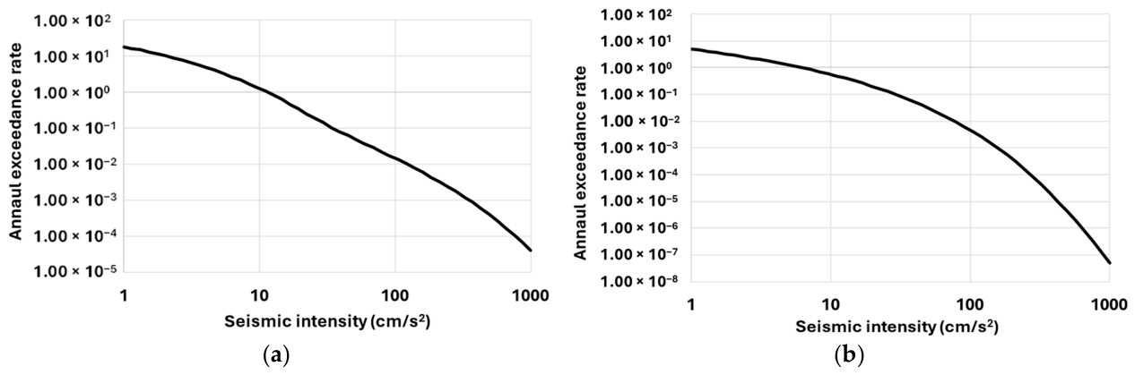
Figure 29a shows the annual PGA exceedance rate λ i m at the bridge site [56]. It was assumed that both capacity and seismic demand are lognormally distributed, resulting in a lognormal distribution for the damage limit state. In the last analysis, the PGA was 0.93 g, which was used as the mean value for the lognormal density function P f | i m . Additionally, the standard deviation of the natural logarithm of capacity and demand was β D 2 + β C 2 = 0.70. The adopted value represents the combined logarithmic dispersion of demand and capacity. For the capacity component, previous studies of reinforced-concrete structures have reported values in the ranges 0.32–0.49 [67], 0.50–0.55 [68], and 0.46 [69]. For the demand component, β D , values between 0.30 and 0.60 have been reported [70], while the present ground-motion suite produced β D = 0.38 0.57 . We therefore adopted β C = 0.525 , corresponding to the midpoint of the upper reported range (0.50–0.55) of capacity dispersion, and β D = 0.475 , corresponding to the midpoint of the range obtained in this study (0.38–0.57). These values give 0.525 2 + 0.475 2 = 0.70 .
The convolution of P f | i m with the annual exceedance rate of PGA yields the bridge’s annual failure rate (Equation (3)). This failure rate served as the basis for calculating the reliability index. After applying these equations, the annual damage rate was λ f = 0.0000246 , the damage probability for a service life of T = 50 years was P f , T = 0.00123 , and the damage reliability index is β f = 3.03 . The 50-year period is used in the reliability calculation as the reference exposure period adopted in this formulation, because it is the standard service life used in all seismic design regulations in Mexico for both bridges and buildings. The study scaled the seismic records based on PGA. Given the bridge’s fundamental period (T1 = 1.4 s), the reliability index was also determined using the exceedance rate for the bridge’s fundamental period, shown in Figure 29b, and the mean pseudo-acceleration of the response spectra for the same period. Applying Equations (1)–(3), the vulnerability index increased to β f = 3.60 . This additional result demonstrates that the reliability estimate is influenced not only by dispersion but also by the spectral characteristics of the selected ground motions and the intensity measure used in the hazard integration.
To evaluate the influence of dispersion on the bridge reliability index, the index was re-evaluated using the lower and upper combinations of the capacity and demand dispersions considered in the study gives combined dispersions of 0.50 2 + 0.38 2 = 0.63 and 0.55 2 + 0.57 2 = 0.79 . The corresponding reliability indices change from the reference value of β f = 3.03 to β f = 3.23 and β f = 2.77 , respectively. Thus, although the reliability index is sensitive to the assumed dispersion, the sensitivity analysis explicitly identifies the range of reliability values associated with the plausible dispersion range.
While β f = 3.03 (using PGA to scale) falls within the wide range reported in the structural reliability literature [71], it is slightly lower than the target benchmark of β f = 3.5   typically specified by modern bridge design codes [45] for the collapse limit state. The results also showed that the seismic response under the design earthquake for a 475-year return period was satisfactory.
The spatial torsion effect on the main beam of a curved bridge during strong earthquakes can substantially change the force distribution between supports and piers if the girders enter an inelastic behavior branch. In a simply supported multi-span system, elastomeric bearings provide flexible rotational boundary conditions that significantly reduce torsional buildup in the main girders compared with continuous superstructures. The primary seismic inertia forces are transmitted directly to the piers through shear and lateral-force mechanisms, with concentrated plastic hinges capturing the bridge’s true nonlinear behavior. However, to verify the elastic assumption in these elements, the combined stress state ( σ x from axial force and bending M m a x , and τ x y from shear V m a x and spatial torsion T m a x acting on the critical AASHTO girder section was evaluated under the maximum response demand. The Von Mises equivalent stress criterion σ v m = σ x 2 + 3 τ x y 2 was used to evaluate the multiaxial stress interaction; σ x is the sum of axial stresses with bending stresses and σ x is the sum of torsion stresses with shear stresses. The maximum equivalent stresses in the girder, under peak seismic actions, ranged from σ v m = 0.3   MPa to σ v m = 8   MPa, which are below the steel yield strength F y = 412   MPa. The combined stress demand remains well within the linear-elastic range.

6.4. Unseating Evaluation

To evaluate the likelihood of unseating failure relative to pier shear failure, the available seat length (Navail) on the hammerhead caps was compared directly with the maximum longitudinal displacement demands (Dlong) from the nonlinear time-history analyses. Dlong was conservatively determined by adding the maximum displacement demand at piers or abutments to the maximum displacement demands at the bearings on them.
The cap beam width is 2.70 m at piers (Figure 3) and 1.80 m at abutments. Considering girder placement, the available seating length per girder is 1.40 m at abutments and 1.00 m at piers. Table 5 summarizes the comparison between longitudinal displacement demands and the available seating length at the collapse seismic intensity.
Table 5 confirms that pier failure is the bridge’s primary collapse mechanism. Maximum longitudinal displacement demands reach at most 45% of the available seat length in piers (DTotal/Navail = 0.45 at Pier 5), and 22% in abutment 1 (DTotal/Navail = 0.22).

7. Conclusions

This study evaluates the expected seismic response of a curved viaduct in Mexico using seismic records from two independent sources. The primary motivation for this research was to analyze an irregular curved bridge designed in accordance with modern seismic regulations. Initially, the numerical model was calibrated using data from an ambient vibration measurement campaign, and a nonlinear analysis was performed to assess seismic performance and failure mechanisms. The results obtained lead to the following conclusions:
The bridge is located in a high-intensity seismic zone. A recent seismic hazard study conducted by this working group determined the expected seismic intensities at the site for various return periods. The primary seismic sources governing the bridge’s dynamic response at its fundamental period (T1 = 1.40 s) are interplate faults and intermediate-depth intraplate faults. Although local crustal sources contribute to short-period intensities (PGA) and their spectral energy at T1 = 1.40 s is negligible, future research should include crustal records to evaluate their possible influence on component-level force demands.
The interplate records imposed higher structural demands than the intraplate records considered in this study. However, these differences should be interpreted as the combined effect of the characteristics of the two ground-motion populations, including source type, magnitude, distance, and spectral content, rather than as an isolated effect of the seismic source. In particular, the higher spectral intensity of the interplate records near the viaduct’s fundamental period increased structural demands on the bridge. A controlled comparison using records conditioned on comparable PGA, Sa(T1), or spectral shape is needed to quantify the independent contribution of source type and remains an important area for future research.
Under the design intensity of a 475-year earthquake, the bridge exhibited satisfactory seismic behavior, with the piers remaining elastic. Although some shear keys reached their maximum strength, the maximum displacement demands were less than 60% of their capacity. The bridge girders are supported by elastomeric bearings with thicknesses of 57 mm and 73 mm. The maximum displacement demand on these elements was in the longitudinal direction of the bridge. In this direction, the intraplate source generated demands below 40% of the bearings’ displacement capacity, whereas interplate seismic records produced demands below 60% of that capacity. Notably, the 57 mm thick bearings experienced the highest demands.
Many structural components sustained damage during the 2500-year earthquake. Most piers had displacement demands below the moderate damage limit state, with only three elements slightly exceeding it. Two shear keys nearly reached their maximum displacement capacity, while the others experienced lower demands. Interplate earthquakes produced longitudinal displacement demands that placed the bearings between the slight and extensive damage limit states. However, none of them exceeded their maximum displacement capacity.
To assess the viaduct’s reliability index, the seismic intensity (PGA) was increased, and the progression of damage was analyzed until shear failure occurred in both the abutments and the shortest pier. At this point, a failure of a group of shear keys on the outer side of the viaduct’s curve was also observed, and several elastomeric bearings exceeded the collapse limit in the longitudinal direction. This behavior confirms that torsional coupling induces severe demand concentrations on the outer-curve bearings and shear keys. Adding seismic restrainers to limit the maximum longitudinal and transverse displacement of the viaduct’s superstructure could reduce the bridge’s seismic vulnerability to extreme events and, where appropriate, increase the piers’ shear capacity. However, any retrofit must be based on detailed nonlinear analyses that demonstrate its effect on the expected seismic response of the viaduct and its foundation. Future studies should incorporate explicit shear-cracking degradation and flexure–shear interaction into the nonlinear model to further investigate their influence on the predicted collapse mechanisms of the bridge.
The reliability assessment also highlighted the importance of considering the spectral intensity at the viaduct’s fundamental period. When the annual exceedance rate and mean pseudo-acceleration corresponding to T1 = 1.40 s were used in the reliability formulation, the reliability index increased from 3.03 (using PGA demands) to 3.60 (using T1 demands). This result reinforces the importance of the spectral characteristics of ground motions near the fundamental period, while the PGA-based scaling adopted in the nonlinear analyses provides a consistent intensity measure across the seismic hazard levels considered. The use of PGA-based scaling is a limitation of the present study, and further research incorporating Sa(T1)-based or spectrum-compatible scaling could provide additional insight into the sensitivity of the seismic response to the selected intensity measure, an appropriate topic for future research. Moreover, developing a multi-component system reliability framework that includes system-level limit states would significantly extend this work and offer a valuable direction for future studies.
Finally, a limitation of this study lies in the large-scale factors (ranging from 7 to 34) required to drive the bridge piers to collapse during the incremental scaling procedure. The accelerogram amplitude was increased without modifying its strong-motion duration or other temporal characteristics. Consequently, cumulative energy dissipation, cyclic degradation, and duration-dependent effects associated with real extreme earthquakes may not be fully represented at very high amplification levels. Consequently, while the calculated reliability index provides a robust benchmark for the pier collapse limit state under the site’s spectral characteristics, future research should incorporate duration-dependent or spectrally matched record selection to further refine failure predictions at extreme intensity levels.

Author Contributions

Conceptualization, J.M.J., B.A.O., G.M. and A.R.S.; methodology, J.M.J. and J.I.L.-P.; software, J.A.; validation, J.M.J., J.A., J.I.L.-P. and B.A.O.; formal analysis, J.A. and J.I.L.-P.; investigation, J.M.J., G.M. and A.R.S.; resources, J.M.J. and J.A.; data curation, J.A.; writing—original draft preparation, J.M.J., B.A.O.; writing—review and editing, J.M.J., B.A.O., G.M., A.R.S. and J.I.L.-P.; visualization, J.A. and J.M.J.; supervision, J.M.J. and B.A.O. All authors have read and agreed to the published version of the manuscript.

Funding

This research received no external funding.

Data Availability Statement

The datasets generated during and/or analyzed during the current study are available from the corresponding author on reasonable request.

Conflicts of Interest

The authors declare no conflict of interest.

References

  1. Basöz, N.; Kiremidjian, A.S. Evaluation of Bridge Damage Data from the Loma Prieta and Northridge, California Earthquakes; Technical Report MCEER-98-0004; University of Buffalo: Buffalo, New York, USA, 1998. [Google Scholar]
  2. Buckle, I.G. The Northridge, California Earthquake of 17 January 1994: Performance of Highway Bridges; Technical Report MCEER-94-0008; University of Buffalo: Buffalo, New York, USA, 1994. [Google Scholar]
  3. Wang, Z.; Lee, G.C. A comparative study of bridge damage due to the Wenchuan, Northridge, Loma Prieta and San Fernando earthquakes. Earthq. Eng. Eng. Vib. 2009, 8, 251–261. [Google Scholar] [CrossRef] [Scilit]
  4. Anderson, L.D.; Mitchell, D.; Tinawi, R.G. Performance of concrete bridges during the Hyogo-ken Nanbu (Kobe) earthquake on 17 January 1995. Can. J. Civ. Eng. 1996, 23, 714–726. [Google Scholar] [CrossRef] [Scilit]
  5. Han, Q.; Du, X.; Liu, J.; Li, Z.; Li, L.; Zhao, J. Seismic damage of highway bridges during the 2008 Wenchuan earthquake. Earthq. Eng. Eng. Vib. 2009, 8, 263–273. [Google Scholar] [CrossRef] [Scilit]
  6. Kawashima, K.; Takahashi, Y.; Ge, H.; Wu, Z.; Zhang, J. Reconnaissance report on damage of bridges in 2008 Wenchuan, China, earthquake. J. Earthq. Eng. 2009, 13, 965–996. [Google Scholar] [CrossRef] [Scilit]
  7. Lin, C.J.; Hung, H.H.; Liu, K.Y.; Chai, J.F. Reconnaissance Observation on Bridge Damage Caused by the 2008 Wenchuan (China) Earthquake. Earthq. Spectr. 2010, 26, 1057–1083. [Google Scholar] [CrossRef] [Scilit]
  8. Wilson, T.; Mahmoud, H.; Chen, S. Seismic performance of skewed and curved reinforced concrete bridges in mountainous states. Eng. Struct. 2014, 70, 158–167. [Google Scholar] [CrossRef] [Scilit]
  9. Serdar, N.; Ulićević, M.; Janković, S. Influence of horizontal curvature radius and bent skew angle on seismic response of RC bridges. Građevinar 2017, 69, 83–92. [Google Scholar] [CrossRef] [Scilit]
  10. Serdar, N.; Folic, R. Ductility displacement ratio in damage analysis of RC curved bridges. In Proceedings of the 16th European Conference on Earthquake Engineering, Thessaloniki, Greece, 18–21 June 2018. [Google Scholar]
  11. Kameshwar, S.; Padgett, J.E. Characterizing and predicting seismic repair costs for bridges. J. Bridge Eng. 2017, 22, 04017083. [Google Scholar] [CrossRef] [Scilit]
  12. Feng, R.; Papadopoulos, S.P.; Yuan, W.; Sextos, A.G. Loss estimation of curved bridges considering the incidence angle and spatial variability of earthquake ground motion. Soil Dyn. Earthq. Eng. 2022, 163, 107523. [Google Scholar] [CrossRef] [Scilit]
  13. Rashid, M.; Nishio, M. Optimal intensity measure-based seismic fragility surfaces for curved bridges considering their sensitivity to seismic excitation direction. Earthq. Eng. Eng. Vib. 2025, 24, 509–526. [Google Scholar] [CrossRef] [Scilit]
  14. Tehrani, P.; Heydarpour, K. Probabilistic evaluation of combination rules for seismic response prediction of horizontally curved RC bridges under varying earthquake incidence angles. Sci. Rep. 2025, 15, 24313. [Google Scholar] [CrossRef] [Scilit] [PubMed]
  15. Bayat, M.; Daneshjoo, F.; Nistico, N. The effect of different intensity measures and earthquake directions on the seismic assessment of skewed highway bridges. Earthq. Eng. Eng. Vib. 2017, 16, 165–179. [Google Scholar] [CrossRef] [Scilit]
  16. Seo, J.; Linzell, D. Nonlinear Seismic Response and Parametric Examination of Horizontally Curved Steel Bridges Using 3D Computational Models. J. Bridge Eng. 2013, 18, 220–231. [Google Scholar] [CrossRef] [Scilit]
  17. Siami, R.; Tehrani, P. Investigating seismic behavior of horizontally curved RC bridges with different types of irregularity in comparison with equivalent straight bridges. Structures 2021, 33, 2570–2586. [Google Scholar] [CrossRef] [Scilit]
  18. Heydarpour, K.; Tehrani, P. Influence of Abutment Stiffness and Strength on the Seismic Response of Horizontally Curved RC Bridges in Comparison with Equivalent Straight Bridges at Different Seismic Intensity Levels. Shock Vib. 2022, 2022, 3532331. [Google Scholar] [CrossRef] [Scilit]
  19. Deshpande, A.; Jagadisha, H.M.; Galagali, A. Parametric study on curved bridges subjected to seismic loading. Int. Res. J. Eng. Technol. 2017, 4, 1883–1889. [Google Scholar]
  20. Amjadian, M.; Agrawal, A. Rigid-Body Motion of Horizontally Curved Bridges Subjected to Earthquake-Induced Pounding. J. Bridge Eng. 2016, 21, 04016090. [Google Scholar] [CrossRef] [Scilit]
  21. Banerjee, S.; Masanobu, S. Experimental verification of bridge seismic damage states quantified by calibrating analytical models with empirical field data. Earthq. Eng. Eng. Vib. 2008, 7, 383–393. [Google Scholar] [CrossRef] [Scilit]
  22. Sakai, J.; Unjoh, S. Earthquake simulation test of circular reinforced concrete bridge column under multidirectional seismic excitation. Earthq. Eng. Eng. Vib. 2006, 5, 103–110. [Google Scholar] [CrossRef] [Scilit]
  23. Sun, Z.; Li, H.; Bi, K.; Si, B.; Wang, D. Rapid repair techniques for severely earthquake-damaged circular bridge piers with flexural failure mode. Earthq. Eng. Eng. Vib. 2017, 16, 415–433. [Google Scholar] [CrossRef] [Scilit]
  24. Jiao, C.; Liu, W.; Wu, S.; Gui, X.; Huang, J.; Long, P.; Li, W. Shake table experimental study of curved bridges with consideration of girder-to-girder collision. Eng. Struct. 2021, 237, 112216. [Google Scholar] [CrossRef] [Scilit]
  25. Cimellaro, G.P.; Reinhorn, A.M.; Bruneau, M. Seismic Resilience of a Health care Facility. In Proceedings of the 2005 Asian-Pacific Network of Centers for Earthquake Engineering Research (ANCER) Annual Meeting, Jeju, Republic of Korea, 10–13 November 2005. [Google Scholar]
  26. Bruneau, M.; Chang, S.E.; Eguchi, R.T.; Lee, G.C.; O’Rourke, T.D.; Reinhorn, A.M.; Shinozuka, M.; Tierney, K.; Wallace, W.A.; Von Winterfeldt, D. A Framework to Quantitatively Assess and Enhance the Seismic Resilience of Communities. Earthq. Spectra 2003, 19, 733–752. [Google Scholar] [CrossRef] [Scilit]
  27. Cimellaro, G.P.; Reinhorn, A.M.; Bruneau, M. Framework for analytical quantification of disaster resilience. Eng. Struct. 2010, 32, 3639–3649. [Google Scholar] [CrossRef] [Scilit]
  28. Gkoumas, K.; Petrini, F.; Bontempi, F. Design for Robustness, Resilience and Anti-Fragility in the Built and Urban Environment: Considerations from a Civil Engineering Point of View. In Proceedings of the 4th International Workshop on Design in Civil and Environmental Engineering, Taipei, Taiwan, 30–31 October 2016. [Google Scholar]
  29. Anwar, G.A.; Dong, Y.; Zhai, C. Performance-Based Probabilistic Framework for Seismic Risk, Resilience, and Sustainability Assessment of Reinforced Concrete Structures. Adv. Struct. Eng. 2020, 23, 1454–1472. [Google Scholar] [CrossRef] [Scilit]
  30. Sartori, S.B. The seismic protection as a key player for structural resilience. In Proceedings of the 18th World Conference on Earthquake Engineering, Milan, Italy, 30 June–5 July 2024. [Google Scholar]
  31. Anwar, G.A.; Dong, Y. Seismic resilience of retrofitted RC buildings. Earthq. Eng. Eng. Vib. 2020, 19, 561–571. [Google Scholar] [CrossRef] [Scilit]
  32. Mina, D.; Karampour, H.; Forcellini, D. Resilience of HP/HT pipelines to combined seismic and thermal loadings. Ocean Eng. 2023, 275, 2023. [Google Scholar] [CrossRef] [Scilit]
  33. Yang, Y.; Huang, H.; Li, G.; Han, B.; Yuan, Z.; Ma, H. A systematic review of resilience assessment and enhancement of urban integrated transportation networks. J. Transp. Geogr. 2025, 129, 2025. [Google Scholar] [CrossRef] [Scilit]
  34. Forcellini, D.; Ranjbar, F.; Asgari, A.; Bagheri, M.; Yazdani, H. Seismic resilience assessment of pile groups against liquefaction-induced lateral spreading: Influence of ground inclination and pile spacing. Eng. Struct. 2026, 360, 122786. [Google Scholar] [CrossRef] [Scilit]
  35. Liao, J.; Forcellini, D.; Fang, J.; Sun, L. An entropy-based multi-criteria approach for intensity measure selection in seismic resilience of structures. Resilient Cities Struct. 2026, 5, 2026. [Google Scholar] [CrossRef] [Scilit]
  36. Abdel-Mohti, A.; Pekcan, G. Seismic response of skewed RC box-girder bridges. Earthq. Eng. Eng. Vib. 2008, 7, 415–426. [Google Scholar] [CrossRef] [Scilit]
  37. Seo, J. Statistical determination of significant curved I-girder bridge seismic response parameters. Earthq. Eng. Eng. Vib. 2013, 12, 251–260. [Google Scholar] [CrossRef] [Scilit]
  38. Maleki-Amin, M.J.; Maalek, S. Regularity classification and corresponding analysis method requirements of horizontally curved bridges with unequal pier heights. Earthq. Eng. Eng. Vib. 2023, 22, 549–571. [Google Scholar] [CrossRef] [Scilit]
  39. Jara, J.M.; Lopez, M.G.; Jara, M.; Olmos, B.A. Rotation and damage Index demands for RC medium-length span bridges. Eng. Struct. 2014, 74, 205–217. [Google Scholar] [CrossRef] [Scilit]
  40. Mosleh, A.; Jara, J.M.; Razzaghi, M.S.; Varum, H. Probabilistic seismic performance analysis of RC bridges. J. Earthq. Eng. 2020, 24, 1704–1728. [Google Scholar] [CrossRef] [Scilit]
  41. Mosleh, A.; Razzaghi, M.S.; Jara, J.M.; Varum, H. Development of fragility curves for RC bridges subjected to reverse and strike-slip seismic sources. Earthq. Struct. 2016, 11, 517–538. [Google Scholar] [CrossRef] [Scilit]
  42. SVS. ARTeMIS Modal Pro, version 4.0; Structural-Vibration-Solutions: Aalborg, Denmark, 2015.
  43. CSI. SAP2000, V24.0; Computer and Structures Inc.: Berkeley, CA, USA, 2022.
  44. CSI. PERFORM 3D, V8.0; Computer and Structures Inc.: Berkeley, CA, USA, 2015.
  45. Mander, J.B.; Priestley, M.J.; Park, R. Theoretical stress–strain model for confined concrete. J. Struct. Eng. 1988, 144, 1804–1826. [Google Scholar] [CrossRef] [Scilit]
  46. Park, R.; Paulay, T. Reinforced Concrete Structures, 1st ed.; Wiley: Hoboken, NJ, USA, 1975; pp. 36–45. [Google Scholar]
  47. AASHTO. AASHTO LRFD Bridge Design Specifications, 7th ed.; American Association of State Highway and Transportation Officials: Washington, DC, USA, 2016. [Google Scholar]
  48. Caltrans. Caltrans Seismic Design Criteria; California Department of Transportation: Sacramento, CA, USA, 2009.
  49. Clough, R.; Johnston, S. Effect of stiffness degradation on earthquake ductility requirements. In Proceedings of the 2nd Japan Earthquake Engineering Symposium, Tokyo, Japan, 17–20 October 1966; pp. 195–198. [Google Scholar]
  50. Jara, J.M.; Hernández, E.J.; Olmos, B.A. Effect of epicentral distance on the applicability of base isolation and energy dissipation systems to improve seismic behavior of RC buildings. Eng. Struct. 2021, 230, 111727. [Google Scholar] [CrossRef] [Scilit]
  51. Xiang, N.; Li, J. Effect of Exterior Concrete Shear Keys on the Seismic Performance of Laminated Rubber Bearing-Supported Highway Bridges in China. J. Soil Dyn. Earthq. Eng. 2018, 112, 185–197. [Google Scholar] [CrossRef] [Scilit]
  52. Megally, S.H.; Silva, P.F.; Seible, F. Seismic Response of Sacrificial Shear Keys in Bridge Abutments; Report No. SSRP-2001/23; University of San Diego: La Jolla, CA, USA, 2002. [Google Scholar]
  53. Nielson, G.B. Analytical Fragility Curves for Highway Bridges in Moderate Seismic Zones. Ph.D. Thesis, School of Civil and Environmental Engineering, Georgia Institute of Technology, Atlanta, Georgia, 2005. [Google Scholar]
  54. Suárez, G.; Caballero-Jiménez, G.V.; Novelo-Casanova, D.A. Active Crustal Deformation in the Trans-Mexican Volcanic Belt as Evidenced by Historical Earthquakes During the Last 450 Years. Tectonics 2019, 38, 3544–3562. [Google Scholar] [CrossRef] [Scilit]
  55. Bayona, J.A.; Suárez, G.; Ordaz, M.G. A probabilistic seismic hazard assessment of the Trans-Mexican Volcanic Belt, Mexico based on historical and instrumentally recorded seismicity. Geofísica Int. 2017, 56, 87–101. [Google Scholar] [CrossRef] [Scilit]
  56. Jara, J.M.; Estrada, A.; Gaytán, R.; Olmos, B.A.; Martínez, G. Effect of the seismic source on the probabilistic hazard assessment in a heritage city in Mexico: A case study of Morelia. Nat. Hazards Rev. 2025, 26, 05025002. [Google Scholar] [CrossRef] [Scilit]
  57. Iingen. Database of Seismic Records. 2022. Available online: https://aplicaciones.iingen.unam.mx/AcelerogramasRSM/Inicio.aspx (accessed on 17 October 2022).
  58. Padgett, J.E.; DesRoches, R. Sensitivity of Seismic Response and Fragility to Parameter Uncertainty. J. Struct. Eng. 2007, 133, 1710–1718. [Google Scholar] [CrossRef] [Scilit]
  59. Padgett, J.E.; Nielson, B.G.; DesRoches, R. Selection of optimal intensity measures in probabilistic seismic demand models of highway bridge portfolios. Earthq. Eng. Struct. Dyn. 2008, 37, 711–725. [Google Scholar] [CrossRef] [Scilit]
  60. Kwan, W.P.; Billington, S.L. Unbonded Posttensioned Concrete Bridge Piers. II: Seismic Analyses. J. Bridge Eng. 2003, 8, 102–111. [Google Scholar] [CrossRef] [Scilit]
  61. Shinozuka, M.; Feng, M.Q.; Kim, H.K.; Kim, S.H. Nonlinear static procedure for fragility curve development. J. Eng. Mech. 2000, 126, 1287–1295. [Google Scholar] [CrossRef] [Scilit]
  62. Nielson, G.B.; DesRoches, R. Seismic fragility methodology for highway bridges using a component level approach. Earthq. Eng. Struct. Dyn. 2007, 36, 823–839. [Google Scholar] [CrossRef] [Scilit]
  63. Maghsoudi-Barmi, A.; Khansefid, A.; Khaloo, A.; Moeini, M.E. Probabilistic seismic performance assessment of optimally designed highway bridge isolated by ordinary unbonded elastomeric bearings. Eng. Struct. 2021, 247, 113058. [Google Scholar] [CrossRef] [Scilit]
  64. Hazus. Hazus Earthquake Model Technical Manual; Hazus 5.1; FEMA: Washington, DC, USA, 2022.
  65. Akbarzadeh, M.R.; Pourhanasa, R.; Bahmanpour, A.; Ranjbar, F.; Asgari, A. Multi-dimensional seismic fragility assessment of steel diagrid systems under mainshock–aftershock sequences via vine-copula modeling. Soil Dyn. Earthq. Eng. 2026, 26, 110267. [Google Scholar] [CrossRef] [Scilit]
  66. NTC-Concreto. Norma Técnica Complementaria Para Diseño y Construcción de Estructuras de Concreto; Gobierno de la Ciudad de México: Mexico City, México, 2023. [Google Scholar]
  67. Biskinis, D.; Fardis, N. Flexure-controlled ultimate deformations of members with continuous or lap-spliced bars. Struct. Concr. 2010, 11, 94–109. [Google Scholar] [CrossRef] [Scilit]
  68. Ramanathan, K.; DesRoches, R.; Padgett, J.E. Analytical fragility curves for multispan continuous steel girder bridges in moderate seismic zones. J. Transp. Res. Board 2010, 2202, 173–182. [Google Scholar] [CrossRef] [Scilit]
  69. Stefanidou, S.P.; Kappos, A.J. Methodology for the development of bridge-specific fragility curves. Earthq. Eng. Struct. Dyn. 2017, 46, 73–93. [Google Scholar] [CrossRef] [Scilit]
  70. Jalayer, F.; Cornell, C.A. A Technical Framework for Probability-Based Demand and Capacity Factor Design (DCFD) Seismic Formats; PEER Report 2003/08; University of California Berkeley: Berkeley, CA, USA, 2003. [Google Scholar]
  71. Steenbergen, R.D.J.M.; Rózsás, A.; Vrouwenvelder, A.C.W.M. Target reliability of new and existing structures—A general framework for code making. Heron 2018, 63, 219–242. [Google Scholar]
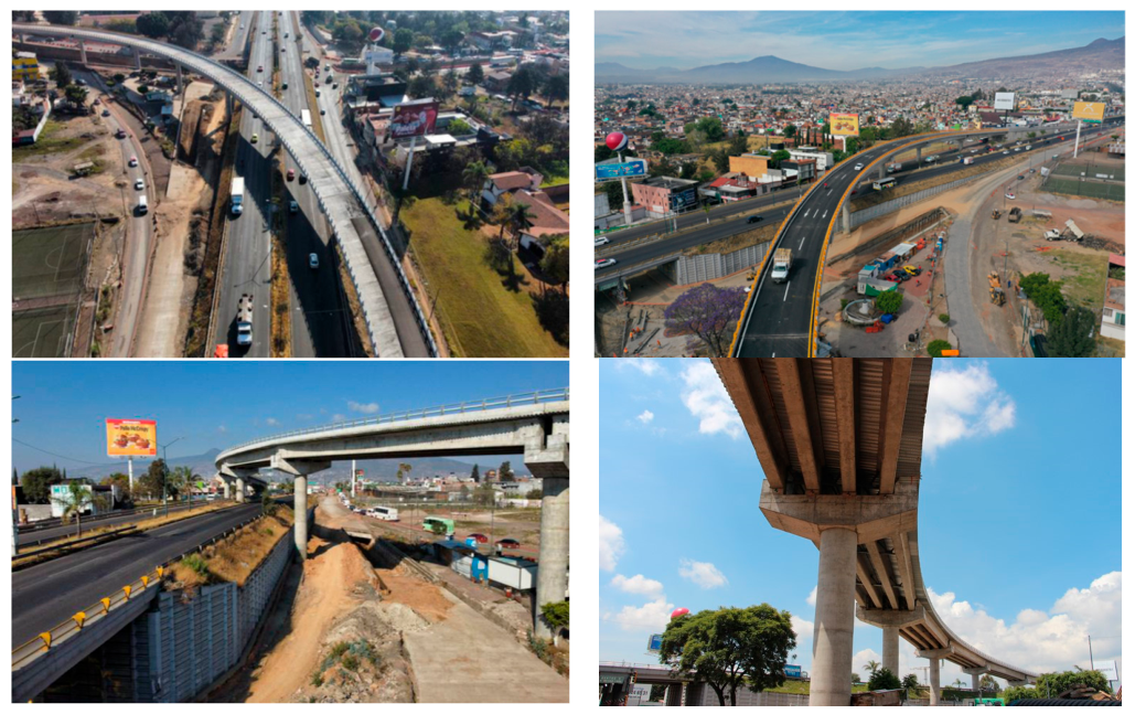
Figure 1. Highway interchange in Morelia. Morelia–Salamanca highway (MEX 43).
Infrastructures 11 00332 g001
Figure 2. Drawing of the curved viaduct and deck slab (in centimeters).
Infrastructures 11 00332 g002
Figure 3. Pier 2 elevation and AASHTO type VI beam (in centimeters).
Infrastructures 11 00332 g003
Figure 4. Campaign of ambient vibration measurements in the viaduct.
Infrastructures 11 00332 g004
Figure 5. Modes identified with ambient vibration measurements. (a) First mode in the transverse direction; (b) second mode in the transverse direction; (c) first bending mode of the slab. Cool colors (blue, green) indicate smaller modal displacements than warm colors (orange, red).
Infrastructures 11 00332 g005
Figure 6. Numerical model created in SAP2000 V24.0 [43].
Infrastructures 11 00332 g006
Figure 7. Modal shapes. (a) First mode in the transverse direction, T = 1.31 s; (b) second mode in the transverse direction, T = 1.16 s; (c) first bending mode on the slab, T = 0.51 s.
Infrastructures 11 00332 g007
Figure 8. Truck axis loadings used to design highway bridges in Mexico. (a) HS-20 truck; (b) T3S3 truck; (c) T3S2R4 truck. The vertical arrow indicates the truck’s total weight.
Infrastructures 11 00332 g008
Figure 9. Backbone curves of the moment–curvature relationship of bridge columns. (a) Pier 2; (b) Pier 5; (c) Pier 8.
Infrastructures 11 00332 g009
Figure 10. Shear key capacity. (a) Pier cap 2, span 1–2; (b) Pier cap 5, span 4–5; (c) Pier cap 8, span 7–8.
Infrastructures 11 00332 g010
Figure 11. Passive action of abutments. (a) Abutment 1; (b) abutment 10.
Infrastructures 11 00332 g011
Figure 12. Disaggregation of the seismic hazard in Morelia. (a) PGA; (b) T = 1.40 s.
Infrastructures 11 00332 g012
Figure 13. (a) Uniform Hazard Spectra at the bridge’s location; (b) spectrum used for the seismic design of the viaduct.
Infrastructures 11 00332 g013
Figure 14. Stockwell Transform of representative ground motions: (a) 2 April 2012 interplate earthquake (M = 6.0); (b) 20 March 2012 interplate earthquake (M = 7.4); (c) 22 May 1997 intraplate earthquake (M = 6.0); (d) 11 December 2011 intraplate earthquake (M = 6.5). The dashed horizontal line denotes the fundamental frequency of the viaduct, f1 = 0.714 Hz (T1 = 1.40 s). Arrows indicate the average frequency of the maximum time-averaged S-transform power.
Infrastructures 11 00332 g014
Figure 15. Scaled response spectra for Tr = 475 years. (a) Interplate earthquakes; (b) intraplate earthquakes. Grey lines are the response spectra for each seismic record; the solid black line is the median response spectrum; and the dashed and dotted lines are the median plus and minus one standard deviation, respectively.
Infrastructures 11 00332 g015
Figure 16. Average of the maximum drift ratios for piers and abutments. (a) Interplate earthquakes; (b) intraplate earthquakes.
Infrastructures 11 00332 g016
Figure 17. Demand/capacity ratios for shear keys of the bridge subjected to intraplate earthquakes. (a) Shear force ratios; (b) displacement ratios.
Infrastructures 11 00332 g017
Figure 18. Demand/capacity ratios for shear keys of the bridge subjected to interplate earthquakes. (a) Shear force ratios; (b) displacement ratios.
Infrastructures 11 00332 g018
Figure 19. Ratio of average displacement demands to sliding displacement of the 57 mm thick bearings. (a) Intraplate earthquakes in the longitudinal direction; (b) interplate earthquakes in the longitudinal direction; (c) intraplate earthquakes in the transverse direction; (d) interplate earthquakes in the transverse direction.
Infrastructures 11 00332 g019
Figure 20. Ratio of average displacement demands to the ultimate displacement of the 57 mm thick bearings. (a) Intraplate earthquakes in the longitudinal direction; (b) interplate earthquakes in the longitudinal direction.
Infrastructures 11 00332 g020
Figure 21. D/H ratios of the 57 mm thick bearings. (a) Intraplate earthquakes in the longitudinal direction; (b) interplate earthquakes in the longitudinal direction.
Infrastructures 11 00332 g021
Figure 22. Average of the maximum drift ratios of piers and abutments. (a) Interplate earthquakes; (b) intraplate earthquakes.
Infrastructures 11 00332 g022
Figure 23. Demand/capacity ratios for shear keys of the bridge subjected to intraplate 2500-year earthquake shaking. (a) Shear force ratios; (b) displacement ratios.
Infrastructures 11 00332 g023
Figure 24. Seismic response of the viaduct during an interplate seismic record. (a) Pier 5 hysteretic loops; (b) shear key on the cap beam of Pier 5.
Infrastructures 11 00332 g024
Figure 25. D/H ratios in the longitudinal direction of the 57 mm thick bearings for a 2500-year return period. (a) Intraplate earthquakes; (b) interplate earthquakes.
Infrastructures 11 00332 g025
Figure 26. Seismic demands on the bridge subjected to interplate seismic records scaled to a peak ground acceleration of 1.8 times the PGA of Tr = 2500 years. (a) Pier drift ratios; (b) displacement demand/capacity ratios for shear keys. Vertical lines show the median ± one standard deviation.
Infrastructures 11 00332 g026
Figure 27. Displacement demands of the 57 mm thick bearings. (a) Mean displacement demand normalized to the capacity of the bearings; (b) D/H ratios. Vertical lines show the median ± one standard deviation.
Infrastructures 11 00332 g027
Figure 28. Shear demand/capacity ratios in columns. Vertical lines show the median ± one standard deviation.
Infrastructures 11 00332 g028
Figure 29. Annual exceedance rate at the bridge location. (a) PGA; (b) T = 1.4 s.
Infrastructures 11 00332 g029
Table 1. Heights of abutments and piers, longitudinal reinforcement in columns, and span lengths.
ElementHeight (m)As (cm2)Span LengthSpan Length (m)
Abutment 14.71243.21Abutment 1–Pier 242.85
Pier 28.46608.05Pier 2–Pier 342.98
Pier 38.12608.05Pier 3–Pier 441.94
Pier 47.84608.05Pier 4–Pier 538.98
Pier 514.76950.08Pier 5–Pier 636.17
Pier 614.06950.08Pier 6–Pier 732.47
Pier 712.44950.08Pier 7–Pier 842.95
Pier 818.40770.20Pier 8–Pier 942.98
Pier 96.20770.20Pier 9–Abutment 1042.88
Abutment 102.82243.21
Table 2. Experimental and numerical frequencies of the bridge.
Mode No.Mode
Description
Experimental
f e x p (Hz)
Numerical
f n u m (Hz)
Relative
Error (%)
MAC Value
11st Transverse mode
(Piers 3–7)
0.7810.7632.30%0.92
22nd Transverse mode
(Piers 5–7)
0.8790.8621.93%0.89
31st Slab vertical Bending 1.9611.9610.01%0.88
Table 3. Moment–curvature parameters that define plastic hinges.
ElementYULRX
øYMYøUMUøLMLøRMRøXMX
(rad/m)(kN-m)(rad/m)(kN-m)(rad/m)(kN-m)(rad/m)(kN-m)(rad/m)(kN-m)
Abutment 10.0022954440.0243073260.1220060500.134907110.14839711
Pier 20.0017918,2180.0133024,1330.0789019,8020.087805420.09710542
Pier 30.0017918,1640.0133024,0880.0789019,8330.087801700.09710170
Pier 40.0017818,0720.0134023,8630.0789019,9090.087803840.09710384
Pier 50.0018624,9710.0129033,5770.0881033,1210.0974059120.107145912
Pier 60.0018524,7170.0130033,4110.0881033,2040.0974072710.107147271
Pier 70.0018524,7820.0130033,4590.0881033,1820.0974061790.107146179
Pier 80.0018321,5460.0125028,5630.0789025,2980.0878011350.097101135
Pier 90.0018221,0890.0127028,2660.0834025,7030.0971024090.106812409
Abutment 100.0022553090.0247072440.1220060720.1349013120.148391312
Table 4. Shear capacity and demand of columns.
ElementDiameterAgAs longLong RebarPuVcVsVCVDVD/VC
(m)(m2)(m2)%(kN)(kN)(kN)(kN)(kN)-
Abutment 11.501.770.0243210.013832472150471262130701.17
Pila 22.003.140.0608050.019495683822628444933840.76
Pila 32.003.140.0608050.019494393822628444939610.89
Pila 42.003.140.0608050.019491373822628444942670.96
Pila 52.003.140.0950080.030294933822628444926030.58
Pila 62.003.140.0950080.030289103822628444935380.80
Pila 72.003.140.0950080.030290613822628444943340.97
Pila 82.003.140.077020.024510,3773822628444921230.48
Pila 92.003.140.077020.024593963822628444953101.19
Abutment 101.501.770.0243210.013829562150471262130381.16
Table 5. Comparison of longitudinal displacement demands with available seating length at piers and abutments at the collapse seismic intensity.
Substructure
Element
Heigth
H(m)
Max Long DriftMax
Column Displ (m)
Max
Drift
Bearing
Max
Bearing
Displ (m)
DTotal (m)Navail (m)Ratio
DTotal/Navail
Abutment 14.710.0030.0125.1520.2900.3101.400.218
Pier 28.460.0110.0935.2910.3000.3901.000.395
Pier 38.120.0120.0945.0360.2900.3801.000.381
Pier 47.840.0110.0834.7130.2700.3501.000.351
Pier 514.760.0190.2812.9700.1700.4501.000.450
Pier 614.060.0170.2321.3310.0800.3101.000.308
Pier 712.440.0180.2241.2930.0700.3001.000.298
Pier 818.400.0120.2271.1710.0700.2901.000.294
Pier 96.200.0090.0581.3260.0800.1301.000.134
Abutment 102.820.0010.0021.8110.1000.1101.400.075
Disclaimer/Publisher’s Note: The statements, opinions and data contained in all publications are solely those of the individual author(s) and contributor(s) and not of MDPI and/or the editor(s). MDPI and/or the editor(s) disclaim responsibility for any injury to people or property resulting from any ideas, methods, instructions or products referred to in the content.