Establishing an In-Situ Baseline Mechanical Monitoring Framework for Asphalt Pavements Using Embedded Strain Sensors

Abstract

Asphalt pavements undergo progressive mechanical changes during service life due to traffic loading, temperature variations, moisture and material ageing. Embedded strain sensors can support in-situ pavement performance monitoring, but their response is strongly affected by experimental variables that must be identified before reliable long-term ageing indicators can be established. This study establishes an in-situ baseline mechanical monitoring framework for asphalt pavements using embedded resistive strain transducers. KM-100HAS sensors were installed in an asphalt test section and evaluated through controlled field campaigns. A 17-point cross-pattern loading procedure was used to validate sensor location and orientation after construction. Load-free monitoring windows were analysed to estimate strain–temperature sensitivity and assess thermal correction of static loading–recovery tests. The results showed that loading position strongly conditions the measured strain response. Passive monitoring indicated that strain–temperature sensitivity depends on both temperature level and sensor location. In the mechanical tests, normalization of the recovery branch and logarithmic fitting over the first 200 s provided a consistent recovery-shape descriptor. The resulting slope, $b_{\mathrm{l}\mathrm{o}\mathrm{g}200}$, showed a strong linear relationship with the recovery percentage after 10 min (R² = 0.855). The proposed workflow provides a standardized baseline protocol for asphalt pavement monitoring and its mechanical evolution.

1. Introduction

Asphalt pavement is the most widely used pavement type worldwide, mainly due to its favourable load-bearing capacity, riding comfort, ease of construction and maintenance efficiency [1]. The bitumen (typically around 5 wt%) provides the viscoelastic behaviour that allows asphalt mixtures to accommodate traffic loading and environmental variations; consequently, asphalt concrete should be considered a temperature-sensitive viscoelastic–plastic material rather than a purely elastic one. Its mechanical response depends on temperature, loading conditions, loading speed and interface conditions [2,3].

During service life, asphalt materials inevitably undergo ageing, understood as the combined result of physical changes and chemical reactions within the material [2]. Long-term exposure to oxygen, solar radiation, temperature variations and moisture leads to irreversible physicochemical changes in the asphalt matrix [1]. As ageing progresses, the material tends to harden and become more brittle, increasing its susceptibility to cracking under traffic loading [1,2]. Thus, pavement performance depends on a balance between stiffness and deformability: excessive softness favours rutting and permanent deformation, whereas excessive hardening promotes brittleness and cracking [2].

Early, continuous and effective monitoring is essential to improve pavement management, reduce maintenance costs and extend the service life of road infrastructure. Pavement monitoring has evolved from manual, destructive or discontinuous inspection methods towards automated vehicle-mounted systems, embedded sensing technologies and wireless sensor networks. These systems allow variables such as strain, pressure, temperature and moisture to be monitored, providing information that cannot be fully captured through surface-based inspections alone [4].

From a mechanical monitoring perspective, asphalt deterioration can be interpreted through deformation and recovery behaviour, using the conceptual framework of the Multiple Stress Creep Recovery test [5].

Previous works have demonstrated the potential of in-situ and full-scale pavement monitoring to measure strains, stresses, deflections, moisture and temperature under real or controlled loading conditions [3,6,7,8,9,10,11]. Accelerated pavement testing has also shown the value of using strain gauges, accelerometers, profilometers and falling weight deflectometer measurements to evaluate deformation and structural condition, although the effects of time, climate and ageing are difficult to accelerate realistically [12]. Numerous studies have explored the versatility in accurately measuring temperature and strain of advanced technologies like FBG sensors [13,14,15]. In addition, Rebelo et al. highlighted the sensitivity of embedded sensor measurements to load position, reporting that a 50 mm difference in the load position may cause variations of about 20–25% in the measured strains [14]. Recent developments in self-sensing asphalt mixtures have shown potential for traffic monitoring, while also highlighting the need for recalibration as stiffness and damage evolve during service life [16,17]. Despite these advances, long-term real-scale applications remain limited, and further validation is still needed regarding sensor durability, environmental effects, installation robustness, cost and the use of monitoring data to estimate stiffness degradation over time [4,18,19].

The aim of this work is to establish an in-situ baseline mechanical monitoring framework, identifying and assessing the key experimental variables that govern embedded strain measurements in asphalt pavements. The present work does not propose a new sensor technology or a completed ageing model. Its specific innovation is the integration of four field-control steps within a single baseline workflow: (i) post-construction verification of sensor location and orientation using a local strain-response map; (ii) sensor-specific characterization and correction of thermal drift from load-free windows; (iii) standardized static wheel loading followed by a controlled recovery period; and (iv) extraction of a normalized early-recovery descriptor for later within-section comparison.

2. Materials and Methods

The experimental programme was designed to establish a baseline for interpreting strain measurements obtained from sensors embedded in asphalt pavements under field conditions. It does not quantify ageing-related evolution. Instead, it evaluates the variables that must be controlled before repeated measurements can be compared, including sensor location, pavement temperature, loading position, loading duration and recovery time. The working hypothesis is that deformation–recovery behaviour recorded by embedded resistive strain transducers can provide standardized field-scale descriptors when these experimental variables are explicitly controlled.

The monitoring programme combined load-free thermal observation windows with repeated controlled static wheel-loading tests. Asphalt strain was measured using KM-100HAS asphalt-embedment strain transducers manufactured by Tokyo Sokki Kenkyujo Co., Ltd., Tokyo, Japan. Loading was applied using one front wheel of a Volkswagen ID.3 carrying an 85 kg driver, corresponding to an estimated nominal static wheel load of approximately 4.5 kN. The same electric vehicle, front wheel and driver were used throughout the programme. The loading scenario was selected as a safe and readily reproducible light-vehicle field excitation for relative strain–recovery comparisons. It was not intended to reproduce the impulse generated by a falling weight deflectometer, a heavy-truck axle load or traffic-induced fatigue, and the nominal load was not used to back-calculate structural modulus.

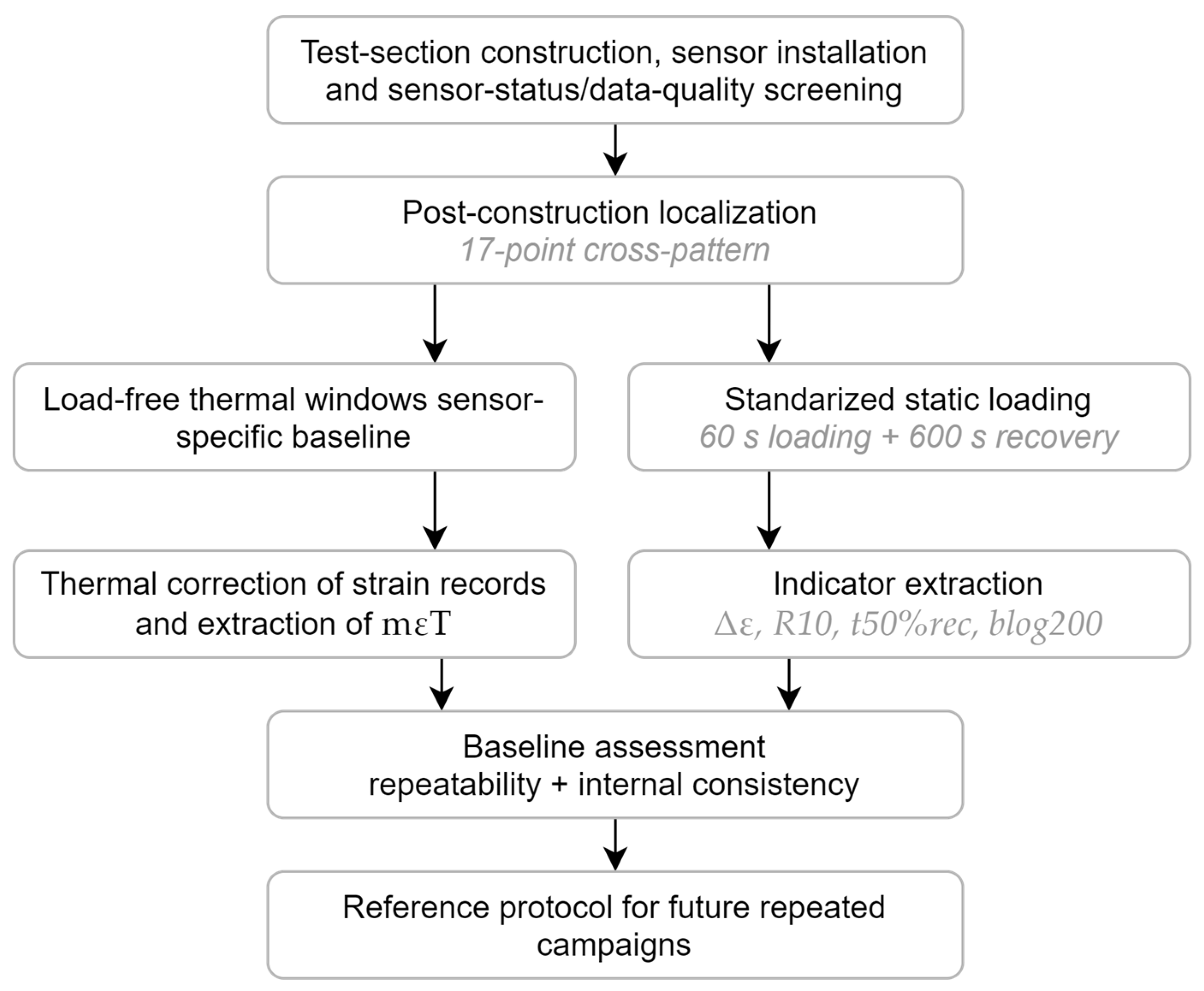
The resulting dataset was used to assess post-construction sensor localization, strain–temperature sensitivity, thermal correction of the recorded strain signals, and the extraction of deformation–recovery indicators from in situ measurements. The experimental workflow therefore addressed both the mechanical response produced by controlled loading and the apparent strain variations generated by the thermo-mechanical interaction between the sensors and the surrounding asphalt mixture. The field campaigns supporting the present baseline were conducted between December 2025 and July 2026. Although measurements were obtained on several dates, they were pooled to characterize the testing framework; no temporal trend was interpreted as pavement ageing. The complete workflow is summarized in Figure 1.

Figure 1. Research workflow used to establish the baseline in-situ monitoring framework.

Figure 1. Research workflow used to establish the baseline in-situ monitoring framework.

2.1. Test Section and Sensor Installation

The instrumented test section was located on the access road to a construction and demolition waste (CDW) recycling facility in Astigarraga, Gipuzkoa, Basque Country, Spain. The pavement was constructed on 15 July 2024. The instrumented section consisted of a 6 cm surface course placed over a 6 cm intermediate course. Both layers were constructed using continuously graded hot-mix asphalt containing 30% reclaimed asphalt pavement (RAP).

The strain transducers were installed at mid-depth within the intermediate course, corresponding to a depth of approximately 9 cm below the pavement surface. This position was selected to obtain a mechanically representative response from the asphalt layer while protecting the sensors from direct contact with traffic loads and from potential damage during pavement construction.

Four KM-100HAS strain transducers, identified as c1–c4, and two pavement-temperature probes were installed. All four strain channels remained electrically responsive, but their suitability for the different analyses varied (Table 1). Sensor c1 was selected for the controlled mechanical tests because its operational loading coordinate and orientation were successfully established through cross-pattern mapping and it provided the most complete set of standardized loading–recovery cycles. Given the duration of each loading–recovery sequence, the mechanical programme was concentrated on one sensor to obtain a sufficiently large within-sensor dataset rather than a smaller number of cycles distributed across several sensors. Sensor c3 was retained for the passive thermal analysis because it provided stable and highly linear strain–temperature records across the selected load-free windows, thereby providing a second sensor location for comparison. Sensor c2 remained operational but showed a weaker and less stable linear strain–temperature relationship and only limited standardized mechanical data. Sensor c4 produced weak responses during localization tests and later exhibited intermittent signal excursions and reduced baseline stability; consequently, it was not used for the quantitative baseline analyses. No complete sensor failure was identified, and the exclusions were based on data continuity, signal stability and suitability for the corresponding analysis. The strain and temperature signals were continuously recorded by a data acquisition unit. Individual measurements were acquired at intervals ranging from 4 to 6 s, corresponding to an effective sampling frequency of approximately 0.17–0.25 Hz. This acquisition rate was sufficient for the static loading–recovery tests and for the analysis of relatively slow temperature-induced strain variations, although it was not intended to characterize the dynamic response generated by moving traffic.

Table 1. Status, data quality, and analytical use of the installed strain and temperature sensors.

Sensor	Status	Use in This Study
c1	Stable; location validated; complete loading dataset	Mechanical and passive thermal analyses
c2	Operational; weaker thermal linearity; limited mechanical dataset	Not included in quantitative baseline
c3	Stable thermal response; location subsequently validated	Passive thermal comparison
c4	Weak localized response; intermittent instability/noise	Not included in quantitative baseline
T1	Operational; temperature channel retained in the consolidated monitoring dataset	Common pavement-temperature reference for thermal correction and temperature-band analyses
T2	Installed; not retained in the consolidated dataset used for the present analyses	Not included in the quantitative baseline

Table 1. Status, data quality, and analytical use of the installed strain and temperature sensors.

Sensor	Status	Use in This Study
c1	Stable; location validated; complete loading dataset	Mechanical and passive thermal analyses
c2	Operational; weaker thermal linearity; limited mechanical dataset	Not included in quantitative baseline
c3	Stable thermal response; location subsequently validated	Passive thermal comparison
c4	Weak localized response; intermittent instability/noise	Not included in quantitative baseline
T1	Operational; temperature channel retained in the consolidated monitoring dataset	Common pavement-temperature reference for thermal correction and temperature-band analyses
T2	Installed; not retained in the consolidated dataset used for the present analyses	Not included in the quantitative baseline

To ensure consistency across monitoring campaigns, all thermal corrections and temperature-clustered analyses were referenced to the same temperature channel, T1. T2 was not included in the consolidated dataset used for the quantitative analyses; its exclusion should not be interpreted as evidence of sensor failure.

The resistive strain transducers operate by converting strain-induced dimensional changes into variations in electrical resistance. Before field installation, the sensors were evaluated under laboratory loading to verify signal linearity, sensitivity, and stability. During installation, particular attention was paid to sensor depth, orientation, and mechanical coupling with the surrounding asphalt to obtain representative strain transfer while maintaining sensor integrity during placement and compaction.

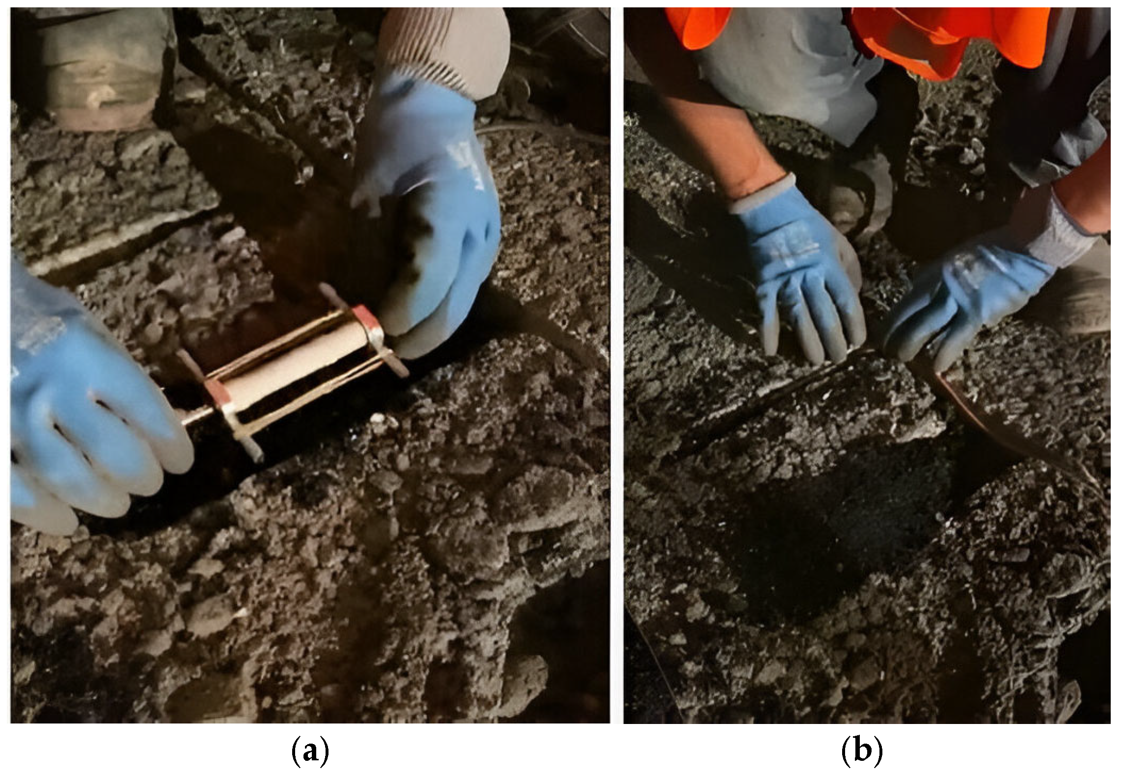
As shown in Figure 2, grooves were formed in the intermediate asphalt course to accommodate the transducers. Each sensor was positioned and aligned within its corresponding groove before being covered and embedded. The surface course was subsequently placed and compacted over the instrumented intermediate layer.

Figure 2. Installation of the asphalt strain transducers: (a) positioning and alignment of a transducer in a groove formed in the intermediate course; (b) final embedding of the transducer before placement and compaction of the surface course.

Figure 2. Installation of the asphalt strain transducers: (a) positioning and alignment of a transducer in a groove formed in the intermediate course; (b) final embedding of the transducer before placement and compaction of the surface course.

2.2. Cross-Pattern Method for Post-Construction Sensor Localization

The cross-pattern method was used as a post-construction localization procedure for the embedded strain sensors. Since paving and compaction may slightly displace the sensors from their nominal installation coordinates, controlled static wheel loads were applied around the expected sensor position to obtain a local strain-response map.

The procedure consisted of a 17-point loading grid defined around the nominal sensor position. The cross-pattern loading scenario was specifically developed as a post-construction sensor-localization procedure rather than as a structural loading test intended to reproduce standardized pavement loading conditions. Instead, a real wheel load was applied statically at successive positions around the expected sensor coordinates to map the local strain field. Loading points were arranged along the sensor-sensitive and perpendicular axes, with 7 cm spacing between adjacent positions in the central area and additional lateral points to better characterize the transition between tensile and compressive response. A 15 cm × 15 cm neoprene pad was placed under the wheel during each load application to delimit the contact area and improve repeatability. The 7 cm spacing was selected relative to the pad dimensions, since this displacement approximately shifts the sensor from the central region of the loaded area towards its edge. This configuration allowed both centred and edge-loading conditions to be examined, while changes in strain magnitude and sign along the two axes were used to infer the sensor location and orientation.

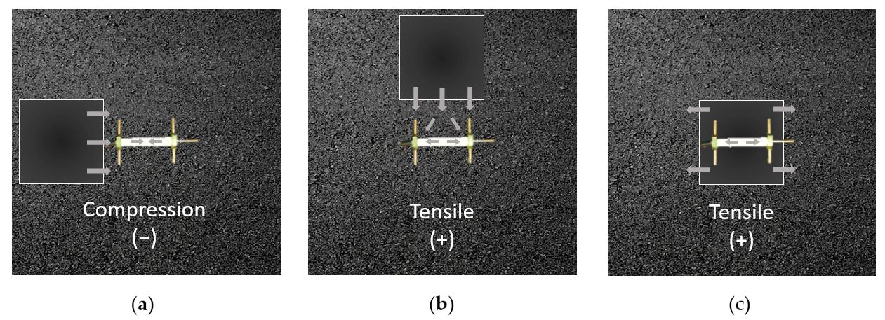
The actual sensor position was identified from the loading points producing the most coherent response, considering both strain magnitude and strain sign. The sign of the measured deformation was used as an orientation criterion (Figure 3). According to the expected deformation mechanism, loading positions aligned with the sensor-sensitive axis generated tensile strain, whereas lateral loading positions generated compressive strain. Therefore, the cross-pattern method allowed both the actual location and the orientation of the embedded sensors to be validated after construction.

Once the sensor location was confirmed, the corrected coordinates were used as reference positions for the subsequent in-situ mechanical characterization tests. This procedure was conceived as a post-construction quality-control step, ensuring that later loading tests were applied at the actual sensor position rather than at the nominal installation coordinates.

Figure 3. Conceptual cross-pattern loading procedure and expected deformation mechanisms: (a) lateral loading position generating compression; (b) loading position along the sensor-sensitive axis generating tensile strain; (c) centred loading position above the sensor.

Figure 3. Conceptual cross-pattern loading procedure and expected deformation mechanisms: (a) lateral loading position generating compression; (b) loading position along the sensor-sensitive axis generating tensile strain; (c) centred loading position above the sensor.

2.3. Testing Methodology and Models

The proposed methodology combines two complementary approaches for monitoring the mechanical evolution of the asphalt layer: a thermal-dependence model based on load-free strain–temperature fluctuations, and a controlled static-loading procedure designed to obtain repeatable strain–recovery parameters.

First, the thermal dependence of the strain signal was evaluated for each sensor and test campaign. The baseline strain recorded by the embedded sensors was affected by daily pavement temperature variations. Therefore, before each controlled loading sequence, a load-free time window was selected and used to estimate the local strain–temperature sensitivity. In this interval, strain variations were assumed to be mainly governed by temperature, since no external mechanical load was applied. A linear relationship was fitted according to:

$$\epsilon \left(t\right)={\epsilon }_0+m_{\epsilon T}\hspace{0.17em}T\left(t\right)$$

(1)

where ε(t) is the measured strain, T(t) is the measured temperature, ${\mathit{\epsilon }}_{\mathit{0}}$ is the fitted intercept, and m_εT is the strain-temperature sensitivity coefficient.

Only the slope $m_{\epsilon T}$ was retained for thermal correction, because the purpose was to remove relative strain fluctuations induced by temperature variations during each monitoring window rather than to estimate the absolute strain level. The corrected signal was calculated as:

$${\epsilon }_{corr}\left(t\right)={\epsilon }_{meas}\left(t\right)-m_{\epsilon T}\hspace{0.17em}\left[T\right(t)-T_{ref}]$$

(2)

where ${\epsilon }_{corr}\left(t\right)$ is the temperature-corrected strain and $T_{ref}$ is the reference temperature of the corresponding loading sequence.

Although this correction is required to isolate the mechanical response during the loading tests, the strain–temperature sensitivity coefficient was also retained as a potential passive monitoring variable. The working hypothesis is that the thermo-mechanical coupling between asphalt and embedded sensors may evolve as the mixture hardens and loses deformability over time. Therefore, $m_{\epsilon T}$ was considered not as a direct ageing indicator at this stage, but as a baseline descriptor whose long-term evolution can be compared with the parameters obtained from controlled loading campaigns.

Second, controlled static-loading tests were performed at the validated sensor coordinates. Each test consisted of repeated wheel-load applications followed by recovery periods, generating sawtooth-shaped strain curves. In the standard configuration, three static load applications of 60 s were applied, with 600 s recovery intervals between consecutive loads. This procedure was designed to obtain comparable deformation and recovery indicators under field conditions. In addition to repetitions at the validated sensor position, the loading protocol included slight positional variations around the sensor in order to generate a controlled range of load-induced strain amplitudes and assess the relationship between deformation level and recovery-curve shape.

For each loading cycle, the following conventional deformation–recovery indicators were extracted from the temperature-corrected strain curve (Table 2):

Table 2. Conventional deformation–recovery indicators extracted from the static loading–recovery curves.

Parameter	Formula	Description
Δε	$\mathsf{\Delta }\mathsf{\epsilon }={\epsilon }_{max}$$-{\epsilon }_0$	Load-induced strain amplitude (µε)
R10	R10 = ((εmax − ε10)/(εmax − ε0)) × 100	Percentage of recovery after 10 min
$t_{50\%rec}$	$t$$({\epsilon }_{50\%rec}$$) = t$$({\epsilon }_0$+ (Δε/2))	Time required to recover 50% of the load-induced deformation

Table 2. Conventional deformation–recovery indicators extracted from the static loading–recovery curves.

Parameter	Formula	Description
Δε	$\mathsf{\Delta }\mathsf{\epsilon }={\epsilon }_{max}$$-{\epsilon }_0$	Load-induced strain amplitude (µε)
R10	R10 = ((εmax − ε10)/(εmax − ε0)) × 100	Percentage of recovery after 10 min
$t_{50\%rec}$	$t$$({\epsilon }_{50\%rec}$$) = t$$({\epsilon }_0$+ (Δε/2))	Time required to recover 50% of the load-induced deformation

These parameters provide field-scale deformation–recovery descriptors that can be tracked over time.

In addition to these conventional indicators, a normalized logarithmic recovery parameter was calculated to describe the early shape of the recovery branch independently of the load-induced strain amplitude. For each unloading event, the temperature-corrected recovery phase was normalized and analysed over the first 200 s according to Equation (3):

$$\begin{gathered} r\left(t\right) = \left[{\epsilon }_{corr}\right(t)- {\epsilon }_0]/\Delta \epsilon \\ log r(t) = log a + b_{log200} log t \iff r(t) = a t^{b\_log200} \end{gathered}$$

(3)

where r(t) is the normalized residual strain, ${\epsilon }_0$ is the pre-loading baseline, a is the scale parameter and $b_{\mathrm{l}\mathrm{o}\mathrm{g}200}$ is the logarithmic slope of the normalized recovery curve. Since r(t) decreases with time, $b_{\mathrm{l}\mathrm{o}\mathrm{g}200}$ takes negative values; more negative slopes indicate faster early recovery. Only data with t > 0 and r(t) > 0 were included. The 200 s fitting window was selected to characterize the early recovery regime rather than the complete 600 s recovery period. Inspection of the recovery curves showed that the largest and most systematic strain variation occurred during approximately the first 200 s after unloading, after which the response progressively entered a flatter long-time relaxation regime. In this latter region, the strain variation per unit time was smaller and therefore proportionally more susceptible to residual thermal drift and measurement noise. A sensitivity analysis compared three fitting approaches: the complete 600 s recovery period, a fixed 200 s window, and a variable window ending at 50% recovery. The full 600 s fits produced a median R² of 0.959 and were valid for 30 of the 31 cycles. Fits up to 50% recovery showed the highest median R² (0.989), but the corresponding fitting duration varied substantially between cycles, from 24 to 464 s. The fixed 200 s window retained all 31 cycles and provided consistently high goodness of fit (median R² = 0.977; range 0.923–0.999), while ensuring that the same portion of the recovery process was analysed in every cycle and limiting the influence of the late-time tail. It was therefore selected as the most suitable compromise between fitting quality, temporal consistency and comparability between measurements. Because the numerical value of the logarithmic slope depends on the selected fitting duration, $b_{\mathrm{l}\mathrm{o}\mathrm{g}200}$ should be regarded as a protocol-specific descriptor and should only be compared with measurements processed using the same 200 s window. Under comparable testing conditions, changes in $b_{\mathrm{l}\mathrm{o}\mathrm{g}200}$ may indicate modifications in the delayed viscoelastic recovery behaviour of the asphalt layer. At this stage, however, it is treated as an apparent field-scale recovery descriptor rather than as a constitutive material constant.

The methodology therefore provides two complementary monitoring routes: direct mechanical characterization through controlled loading tests (conventional indicators and logarithmic recovery parameter), and passive thermal monitoring (through the strain–temperature sensitivity coefficient). The comparison between both approaches over successive campaigns is expected to improve the robustness of long-term ageing assessment in instrumented asphalt pavements.

3. Results and Discussion

3.1. Cross-Pattern Method

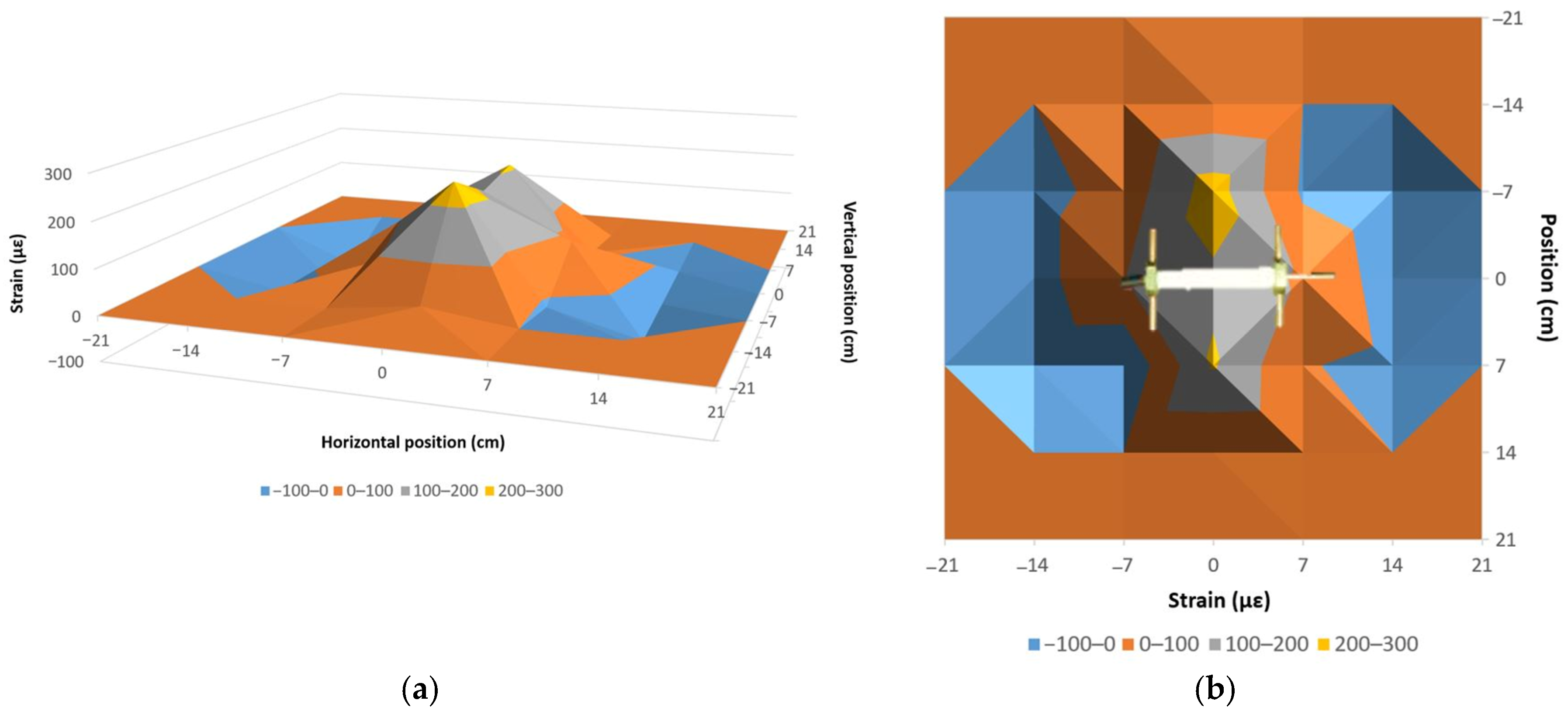
The 17-point cross-pattern test was applied to validate the post-construction location of the embedded strain sensor and to analyse the strain mechanisms generated by different loading positions. Figure 4 shows the strain-response map obtained by applying controlled static wheel loads around the nominal sensor position using the 15 cm × 15 cm neoprene pad. The highest positive responses were concentrated along the central vertical axis, whereas several lateral positions produced lower or negative responses. This distribution is consistent with the expected deformation mechanism described in Section 2.2, where loading positions aligned with the sensor-sensitive axis generate tensile strain and lateral positions generate compressive strain.

The centred loading point produced a tensile response of 185 µε, confirming that the sensor was located within the mapped area. However, the maximum response was not obtained when the neoprene pad was centred directly above the nominal sensor position. The largest value was recorded when the loading point was displaced 7 cm along the vertical axis, reaching 247 µε. A similarly high response was obtained for the opposite 7 cm vertical displacement, with 209 µε. This indicates that the most sensitive loading configuration was not the fully centred position, but the configuration in which the edge of the neoprene pad approximately coincided with the sensor body.

Figure 4. (a) Cross-pattern method results on a 3D diagram (b) Cross-pattern method results on a 2D diagram including a scale representation of the sensor.

Figure 4. (a) Cross-pattern method results on a 3D diagram (b) Cross-pattern method results on a 2D diagram including a scale representation of the sensor.

A plausible mechanical explanation is related to the finite size of the loading area. When the pad is centred directly above the sensor, the stress field transmitted through the asphalt may be more symmetrically distributed around the gauge, producing partial compensation of local deformation components. In contrast, when the edge of the pad is located close to the sensor, the strain field becomes more asymmetric and produces a stronger local tensile response. Therefore, the cross-pattern test not only confirmed the sensor position, but also showed that the relative position between the load-transfer area and the sensor body is a critical variable for repeatable in-situ measurements.

3.2. Effect of Temperature

Temperature variations recorded during the monitoring campaigns produced measurable strain variations in the embedded transducers, even in the absence of externally applied mechanical loads. This response is interpreted as a consequence of the thermo-mechanical coupling between the resistive sensor and the surrounding asphalt matrix. An increase in pavement temperature is associated with thermal expansion of the asphalt layer and may induce apparent compressive strain in the sensor, whereas cooling produces the opposite trend, with apparent tensile strain. Temperature therefore represents an experimental variable that must be evaluated before extracting mechanical indicators from static-loading tests.

3.2.1. Thermal Correction of Strain Curves

Thermal drift must be controlled when interpreting the in-situ mechanical tests, since the wheel-load applications are performed while the pavement temperature is continuously changing. The correction procedure described in Section 2.3 was therefore applied to reduce the temperature-induced strain component from the measured signal before comparing mechanical indicators.

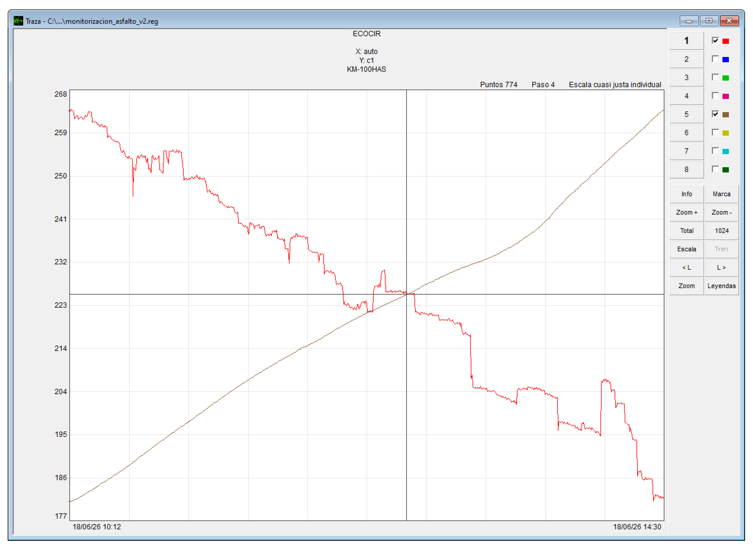
Figure 5 illustrates the magnitude of the thermal effect during a load-free interval. A temperature variation of 1.3 °C over 4 h 18 min generated an apparent compressive strain variation of 82 µε, confirming that thermal drift can reach magnitudes that are relevant for the interpretation of field strain measurements.

Figure 5. Temperature-induced strain during a load-free interval (temperature in brown, strain in red).

Figure 5. Temperature-induced strain during a load-free interval (temperature in brown, strain in red).

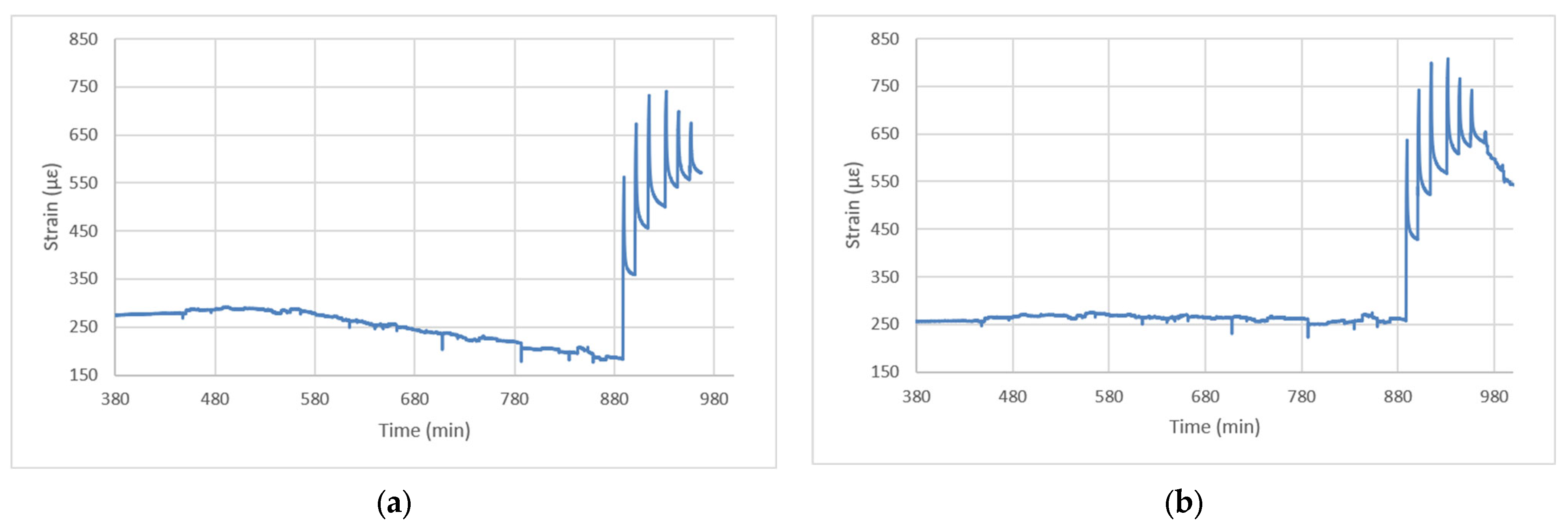
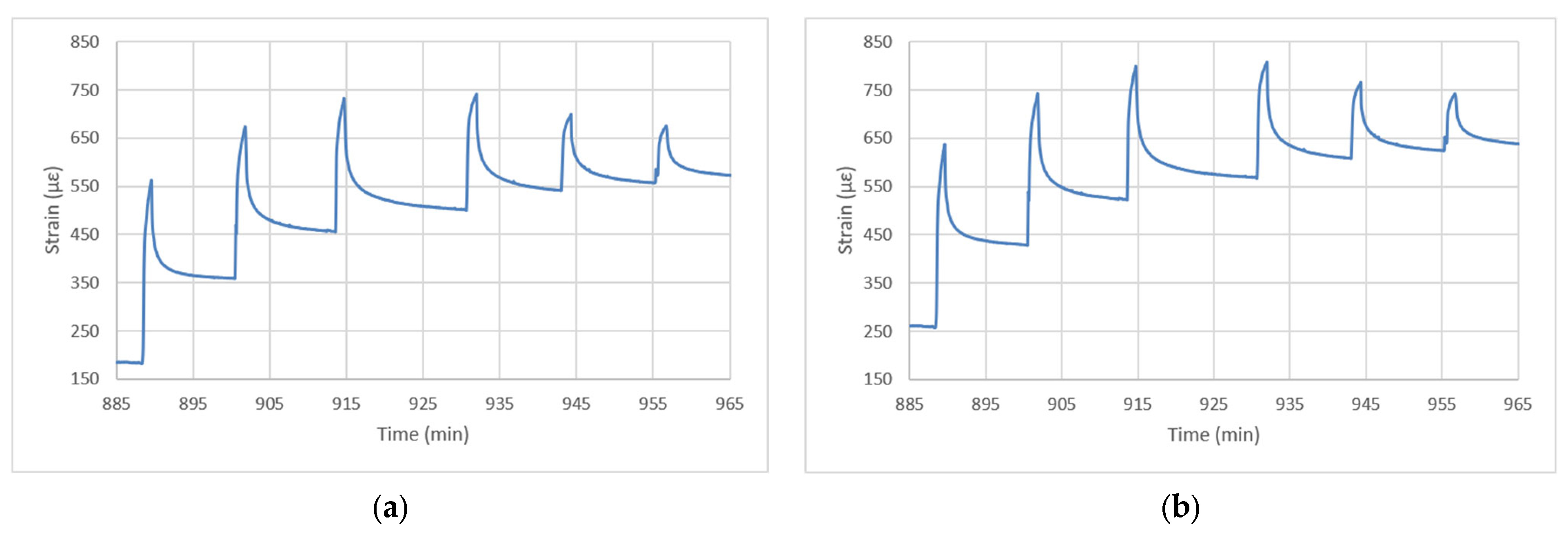
Figure 6 and Figure 7 show the result of applying the thermal correction to a representative mechanical loading sequence. The strain–temperature sensitivity coefficient calculated from the load-free window preceding the loading test was −53.77 µε/°C. The linear fit between strain and temperature, obtained from the data recorded between 06:00 and 13:00 each day before the mechanical loading sequence, showed a coefficient of determination of R² = 0.95. These results indicate that, for the selected interval, the thermal component can be described by a linear model and used to correct the strain signal before parameter extraction.

Figure 6. (a) Measured strain (b) Thermally corrected strain for the selected mechanical loading sequence.

Figure 6. (a) Measured strain (b) Thermally corrected strain for the selected mechanical loading sequence.

Figure 7. (a) Measured strain (b) Thermally corrected strain for six loading measurements analysed.

Figure 7. (a) Measured strain (b) Thermally corrected strain for six loading measurements analysed.

Table 3 compares the indicators obtained from the raw and thermally corrected signals for one representative mechanical loading measurement. The correction produced only minor changes in the direct deformation–recovery indicators: Δε remained practically unchanged, decreasing from 264.29 µε to 263.75 µε; the recovery after 10 min increased from 62% to 64%; and $t_{50\%rec}$ remained constant at 2 min 6 s. This suggests that, for this loading cycle, thermal correction is relevant as a methodological control step, although the main mechanical interpretation remains similar for the raw and corrected signals.

Table 3. Impact of thermal correction on the indicators extracted from one mechanical loading measurement.

Parameter	Raw Signal	Corrected Signal
Δε	264.29 µε	263.75 µε
R10	62%	64%
$t_{50\%rec}$	00:02:06	00:02:06

Table 3. Impact of thermal correction on the indicators extracted from one mechanical loading measurement.

Parameter	Raw Signal	Corrected Signal
Δε	264.29 µε	263.75 µε
R10	62%	64%
$t_{50\%rec}$	00:02:06	00:02:06

3.2.2. Passive Monitoring

In addition to its use as a correction coefficient, the strain–temperature sensitivity coefficient was evaluated as a potential passive monitoring variable. Unlike the controlled static-loading tests, this approach does not require the application of an external mechanical load. Instead, it uses load-free monitoring periods to quantify the apparent strain response induced by natural temperature variations in the asphalt layer.

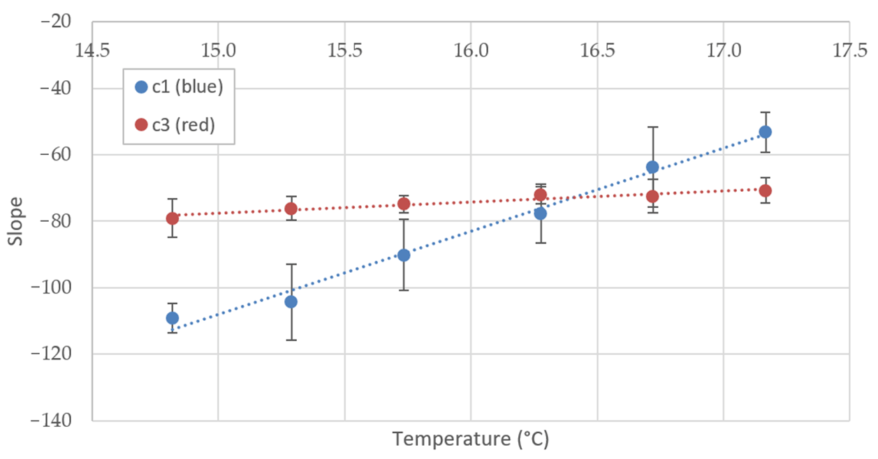
For each available monitoring day, a load-free time window between 06:00 and 13:00 was selected, and a linear regression between temperature and strain was calculated for each embedded sensor (Table 4). The resulting daily slope, $m_{\epsilon T}$, represents the apparent strain variation per unit temperature change. To avoid comparing measurements obtained under different thermal conditions, the daily slopes were grouped according to the mean temperature of each window. In this study, 0.5 °C temperature intervals were used to calculate the mean value and standard deviation of $m_{\epsilon T}$ for each sensor (Figure 8).

Table 4. Temperature-clustered strain–temperature sensitivity coefficients obtained during load-free monitoring windows.

Temperature Interval (°C)	Mean T (°C)	n	c1 Mean Slope (µε/°C)	c1 SD	c3 Mean Slope (µε/°C)	c3 SD
14.5–15.0	14.82	6	−109.19	4.37	−79.05	5.89
15.0–15.5	15.29	36	−104.27	11.42	−76.10	3.48
15.5–16.0	15.73	36	−90.10	10.80	−74.87	2.48
16.0–16.5	16.28	18	−77.72	8.78	−72.16	2.67
16.5–17.0	16.72	17	−63.76	11.98	−72.42	4.94
17.0–17.5	17.17	13	−53.23	6.07	−70.74	3.80

Table 4. Temperature-clustered strain–temperature sensitivity coefficients obtained during load-free monitoring windows.

Temperature Interval (°C)	Mean T (°C)	n	c1 Mean Slope (µε/°C)	c1 SD	c3 Mean Slope (µε/°C)	c3 SD
14.5–15.0	14.82	6	−109.19	4.37	−79.05	5.89
15.0–15.5	15.29	36	−104.27	11.42	−76.10	3.48
15.5–16.0	15.73	36	−90.10	10.80	−74.87	2.48
16.0–16.5	16.28	18	−77.72	8.78	−72.16	2.67
16.5–17.0	16.72	17	−63.76	11.98	−72.42	4.94
17.0–17.5	17.17	13	−53.23	6.07	−70.74	3.80

Figure 8. Temperature-clustered strain–temperature sensitivity coefficients for sensors c1 and c3 during load-free monitoring windows. Blue and red markers correspond to sensors c1 and c3, respectively. Markers represent the mean slope within each 0.5 °C temperature interval and error bars indicate ± one standard deviation.

Figure 8. Temperature-clustered strain–temperature sensitivity coefficients for sensors c1 and c3 during load-free monitoring windows. Blue and red markers correspond to sensors c1 and c3, respectively. Markers represent the mean slope within each 0.5 °C temperature interval and error bars indicate ± one standard deviation.

The results show that the strain–temperature sensitivity was not constant over the analysed temperature range. For sensor c1, the mean slope became progressively less negative as temperature increased, changing from approximately (−109.2 ± 4.4) µε/°C in the 14.5–15.0 °C interval to (−53.2 ± 6.1) µε/°C in the 17.0–17.5 °C interval. This indicates that the apparent thermal response of this sensor was strongly dependent on the temperature level. Sensor c3 showed a more stable response over the same range, with mean slopes varying from approximately (−79.0 ± 5.9) µε/°C to (−70.7 ± 3.8) µε/°C. The negative sign of the slopes indicates that increasing temperature was associated with an apparent compressive strain response, consistent with the thermal behaviour described in the previous section.

These results highlight the need to interpret passive strain–temperature indicators within controlled temperature bands. Direct comparison of daily slopes obtained at different temperature levels could lead to misleading conclusions, since part of the variation in $m_{\epsilon T}$ is associated with the thermal state itself. Therefore, the temperature-clustered values provide a more suitable baseline for future longitudinal monitoring.

At this stage, $m_{\epsilon T}$ should not be interpreted as a direct ageing indicator. Rather, it represents a passive descriptor of the thermo-mechanical coupling between the embedded sensor and the surrounding asphalt layer. Its long-term evolution, evaluated within comparable temperature intervals and together with the variability observed in the baseline period, may help identify future changes in material stiffness, sensor–asphalt interaction or structural condition. Consequently, passive monitoring is considered a complementary route to the controlled static-loading tests, providing continuous information that can support the future assessment of asphalt pavement mechanical evolution.

3.3. Static Loading-Recovery Response

Once the sensor location had been validated and the thermal component had been characterized, controlled static loading–recovery tests were performed around the validated sensor position. The loading protocol included slight positional variations in the vicinity of the sensor in order to generate a range of load-induced strain amplitudes while maintaining the same general test configuration. All loading cycles included in the quantitative analysis were carried out using the same vehicle, wheel, neoprene pad and loading–recovery sequence. Therefore, the variability observed in Δε was not treated only as experimental scatter, but also as a controlled range of mechanical excitation levels produced by small changes in the relative position between the load-transfer area and the embedded gauge.

Short-term repeatability was evaluated using three consecutive loading cycles applied at the same cross-pattern-defined coordinate during the 17 July 2026 campaign. The pavement temperature remained between 16.597 and 16.604 °C, and the vehicle, wheel, contact pad and loading–recovery sequence were unchanged. The load-induced strain amplitude was 142.10 ± 0.39 µε, corresponding to a coefficient of variation of 0.28%. By contrast, R₁₀ was 74.44% ± 10.59 percentage points (CV = 14.23%), and $t_{50\%rec}$ was 67.3 ± 28.7 s (CV = 42.67%). These results indicate very high repeatability of the imposed strain amplitude at a fixed loading position, while the recovery indicators, particularly the threshold-based $t_{50\%rec}$, were more variable. Repeated cycles are therefore required when establishing baseline recovery descriptors.

This approach is consistent with the results of the cross-pattern method, which showed that the strain response is highly sensitive to the relative position between the load and the sensor body. The controlled static loading–recovery tests were therefore used not only to obtain individual deformation–recovery parameters, but also to evaluate how the recovery response changed over a range of imposed strain amplitudes.

The resulting strain signals showed a characteristic sawtooth-shaped response, with a rapid increase in strain during static loading followed by progressive recovery after unloading. This behaviour is consistent with the viscoelastic response of asphalt mixtures under field conditions and supports the use of deformation–recovery parameters to describe the in-situ mechanical behaviour of the monitored layer.

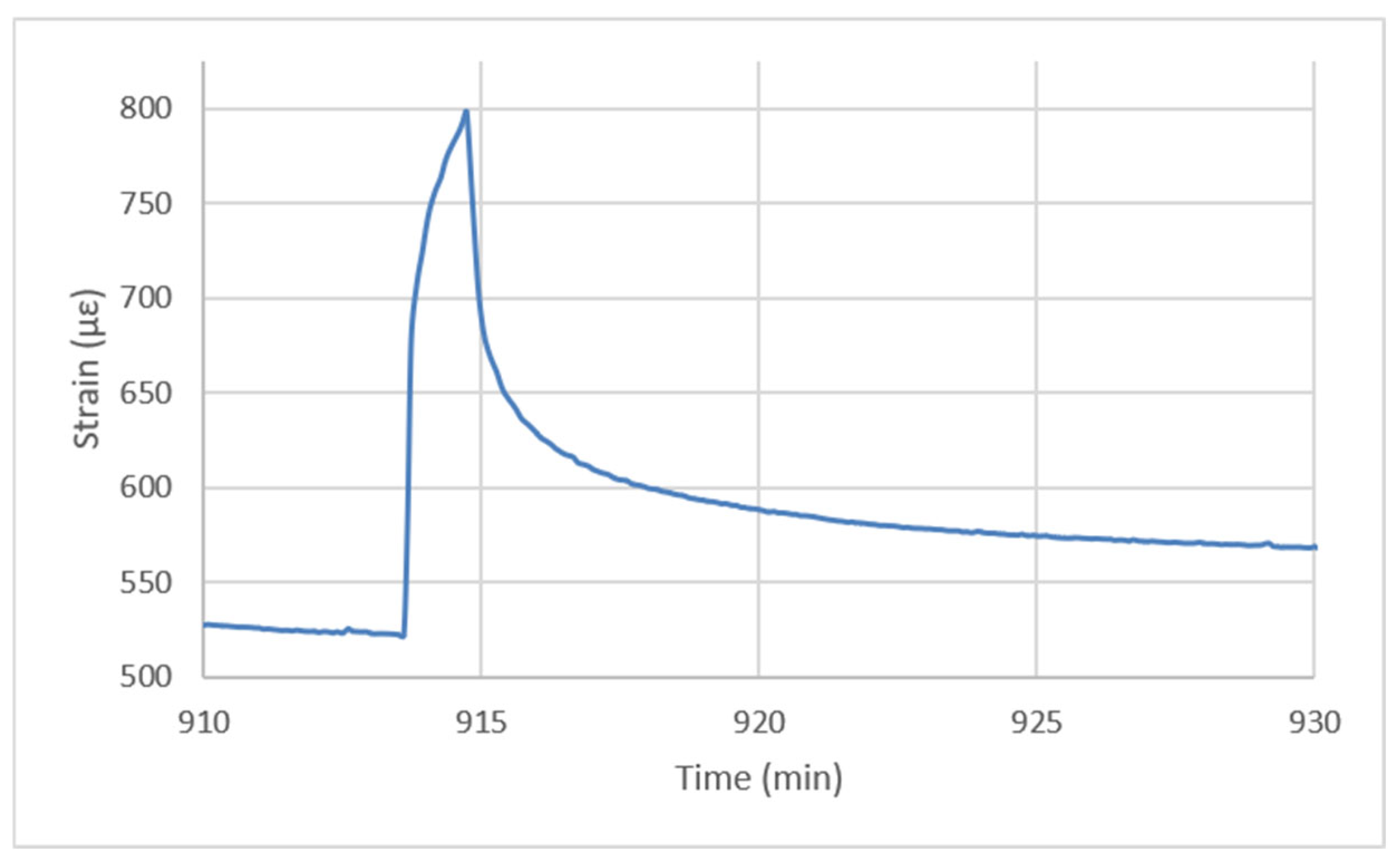
Figure 9 shows a representative thermally corrected strain curve obtained during one static loading–recovery cycle. The curve clearly distinguishes three stages: the pre-loading baseline, the rapid strain increase during load application, and the subsequent recovery branch after unloading. The load-induced strain amplitude, Δε, was obtained from the difference between the baseline strain and the maximum strain reached during loading. The conventional recovery indicators R₁₀ and $t_{50\%rec}$ were calculated from the post-unloading branch.

Figure 9. Representative thermally corrected strain–recovery curve obtained during a controlled static loading test. The test consisted of 60 s of static loading followed by 600 s of recovery.

Figure 9. Representative thermally corrected strain–recovery curve obtained during a controlled static loading test. The test consisted of 60 s of static loading followed by 600 s of recovery.

To compare recovery curves obtained under different strain amplitudes, the post-unloading branches were normalized by Δε and analysed over the first 200 s. This fixed window captured the main early-recovery regime while reducing the influence of the flatter long-time tail and maintaining the same fitting duration across all cycles. For each loading cycle, $b_{\mathrm{l}\mathrm{o}\mathrm{g}200}$ and its associated $R_{200}^2$ were obtained from the log–log fit defined in Section 2.3.

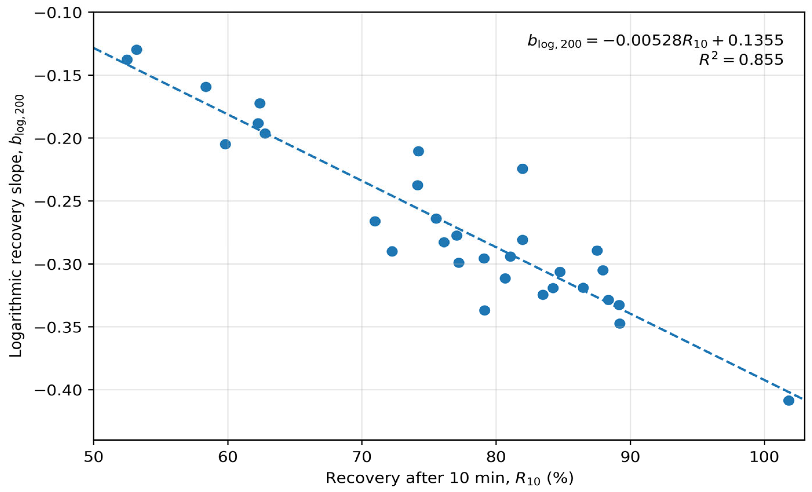
A total of 31 valid loading cycles recorded by sensor c1 across several test days were included in the analysis. Asphalt temperature ranged from 16.60 to 18.64 °C, while $\mathsf{\Delta }\epsilon$ ranged from 25.62 to 378.79 µε, providing a broad range of mechanical excitation levels. The recovery percentage after 10 min ranged from 52.50% to 101.81%, with the value slightly above 100% corresponding to a small recovery overshoot beyond the pre-loading baseline. The logarithmic fits showed consistently high quality, with $R_{200}^2$ values between 0.923 and 0.999 and a median value of 0.977. The resulting $b_{\mathrm{l}\mathrm{o}\mathrm{g}200}$ values ranged from −0.409 to −0.130.

$$b_{\mathrm{l}\mathrm{o}\mathrm{g}200} = -0.00528{\mathrm{R}}_{10} + 0.1355$$

(4)

Figure 10 shows the relationship between $b_{\mathrm{l}\mathrm{o}\mathrm{g}200}$ and R₁₀. Loading cycles with greater recovery after 10 min exhibited more negative early-time slopes, indicating faster initial recovery. The relationship was well described by Equation (4), with $R^2=0.855$ and $p<0.001$. Since $b_{\mathrm{l}\mathrm{o}\mathrm{g}200}$ was calculated over the first 200 s, whereas $R_{10}$ was evaluated after 600 s, the result links the early recovery behaviour with the later extent of recovery. However, both variables were extracted from the same loading–recovery cycle and therefore do not constitute independent measurements. Consequently, the strong relationship observed between them should be interpreted as an internal consistency pattern, indicating that $b_{\mathrm{l}\mathrm{o}\mathrm{g}200}$ captures a component of the recovery behaviour that is also reflected by $R_{10}$, rather than as an independent validation of its sensitivity to pavement mechanical condition or ageing.

Figure 10. Relationship between recovery after 10 min ($R_{10}$) and the signed logarithmic slope of the normalized recovery curve fitted over the first 200 s (b_log200) for 31 controlled static loading-recovery cycles recorded by sensor c1. More negative slopes correspond to faster early-stage recovery. The dashed line represents the linear regression.

Figure 10. Relationship between recovery after 10 min ($R_{10}$) and the signed logarithmic slope of the normalized recovery curve fitted over the first 200 s (b_log200) for 31 controlled static loading-recovery cycles recorded by sensor c1. More negative slopes correspond to faster early-stage recovery. The dashed line represents the linear regression.

The relationship between $b_{\mathrm{l}\mathrm{o}\mathrm{g}200}$ and $t_{50\%rec}$ was moderate ($R^2=0.534$). By contrast, no meaningful dependence was observed between $b_{\mathrm{l}\mathrm{o}\mathrm{g}200}$ and the load-induced strain amplitude, $\mathsf{\Delta }\epsilon$($R^2=0.007$), or between $b_{\mathrm{l}\mathrm{o}\mathrm{g}200}$ and asphalt temperature during the tests ($R^2=0.032$). The absence of a relationship with $\mathsf{\Delta }\epsilon$ indicates that normalization substantially reduced the dependence of the recovery-shape parameter on the initial strain amplitude. However, the apparent weak dependence on asphalt temperature should not be interpreted as evidence of temperature independence, since the mechanical tests covered only a relatively narrow temperature range (16.6–18.6 °C).

At this stage, the relationship between $b_{\mathrm{l}\mathrm{o}\mathrm{g}200}$ and $R_{10}$ provides a baseline characterization of the recovery behaviour of the monitored asphalt layer, rather than providing direct evidence of ageing or separating elastic and viscoelastic mechanisms. Its longitudinal value lies in comparing future measurements obtained under comparable testing conditions with the variability established in the present baseline. Persistent deviations in the individual parameters or in their relationship could indicate changes in pavement response and support the identification of sections requiring complementary mechanical assessment. Longitudinal comparison with independent pavement-condition measurements will nevertheless be required before such deviations can be associated with ageing or damage and translated into maintenance-related decision thresholds.

4. Conclusions

This study established an in-situ baseline field protocol for interpreting strain measurements from sensors embedded in asphalt pavements. Under the tested pavement section, sensor configuration, loading protocol, and temperature conditions, the main conclusions are:

• The 17-point cross-pattern procedure identified the operational loading coordinate and inferred the sensor orientation from the magnitude and sign of the measured response. The centred loading point produced 185 µε, whereas the maximum response reached 247 µε at a 7 cm offset, representing an increase of approximately 34% and quantifying the importance of controlling the relative load position.
• A temperature change of 1.3 °C over 4 h 18 min generated an apparent compressive strain variation of 82 µε. In the representative correction example, Δε changed by approximately 0.2%, R₁₀ by 2 percentage points, and $t_{50\%rec}$ remained unchanged. Thermal correction should therefore be retained as a methodological control step, even when its influence on the direct indicators is limited under a particular test condition.
• Passive strain–temperature sensitivity was sensor-specific. Across the analysed temperature bands, the mean $m_{\epsilon T}$ value for c1 changed from approximately −109.2 to −53.2 µε/°C, whereas c3 remained between approximately −79.0 and −70.7 µε/°C. These ranges establish sensor-specific baseline descriptors of thermo-mechanical coupling and should not be interpreted as ageing indicators at this stage.
• For three consecutive loading cycles applied at the same cross-pattern-defined coordinate, Δε was (142.10 ± 0.39) µε, with a coefficient of variation of 0.28%; R₁₀ was (74.44% ± 10.59) percentage points, with a coefficient of variation of 14.23%; and $t_{50\%rec}$ was (67.3 ± 28.7) s, with a coefficient of variation of 42.67%. This fixed-position subset showed high short-term repeatability of strain amplitude, while the recovery indicators, particularly the threshold-based recovery time, exhibited greater variability.
• For the 31 valid loading cycles recorded by sensor c1, the normalized logarithmic fits over the first 200 s produced $R^2$ values ranging from 0.923 to 0.999, with a median of 0.977. The relationship between $b_{\mathrm{l}\mathrm{o}\mathrm{g}200}$ and R₁₀ reached ($R^2$ = 0.855), showing consistency between the early recovery-curve shape and the later recovery extent. Since both parameters were extracted from the same loading–recovery cycles, this relationship represents internal consistency rather than independent validation or direct evidence of ageing.
• The specific methodological contribution of this study lies in integrating post-construction sensor localization, sensor-specific thermal characterization and correction, standardized static loading–recovery testing, and a normalized early-recovery descriptor within a single field workflow. The resulting parameters and their baseline variability provide a quantitative reference for subsequent monitoring campaigns.

Future work should repeat the protocol during successive monitoring campaigns under comparable loading positions and pavement-temperature ranges and assess changes in $b_{\mathrm{l}\mathrm{o}\mathrm{g}200}$, $R_{10}$, $t_{50\%rec}$, $m_{\epsilon T}$, and in the slope, intercept, and residual dispersion of their relationships. The transferability of the framework should also be evaluated across additional embedded sensors and pavement sections and over a broader range of seasonal temperatures. Comparison with independent structural and material-condition measurements will be required to distinguish changes in pavement behaviour from sensor drift or changes in sensor–asphalt coupling. Only after this longitudinal and cross-sensor validation should persistent deviations from the baseline be associated with ageing or damage and used to establish maintenance-related decision thresholds.

References

1. Zhang, S.; Xiong, K.; Hu, D.; Li, L.; Li, R.; Zhang, J. Molecular mechanisms governing the deterioration of cracking resistance in asphalt induced by aging. Case Stud. Constr. Mater. 2026, 24, e06127. [Google Scholar] [CrossRef] [Scilit]
2. Zhen, T.; Kang, X.; Liu, J.; Zhang, B.; Si, W.; Ling, T. Multiscale Evaluation of Asphalt Aging Behaviour: A Review. Sustainability 2023, 15, 2953. [Google Scholar] [CrossRef] [Scilit]
3. Al-Qadi, I.L.; Loulizi, A.; Elseifi, M.; Lahouar, S. The Virginia Smart Road: The impact of pavement instrumentation on understanding pavement performance. Asph. Paving Technol. 2004, 73, 427–465. [Google Scholar]
4. Di Graziano, A.; Marchetta, V.; Cafiso, S. Structural health monitoring of asphalt pavements using smart sensor networks: A comprehensive review. J. Traffic Transp. Eng. (Engl. Ed.) 2020, 7, 639–651. [Google Scholar] [CrossRef] [Scilit]
5. Federal Highway Administration. The Multiple Stress Creep Recovery (MSCR) Procedure; Technical Brief FHWA-HIF-11-038; Office of Pavement Technology, Federal Highway Administration: Washington, DC, USA, 2011. [Google Scholar]
6. Duong, N.S.; Blanc, J.; Hornych, P. Analysis of the behavior of pavement layers interfaces from in situ measurements. In Bearing Capacity of Roads, Railways and Airfields: Proceedings of the 10th International Conference on the Bearing Capacity of Roads, Railways and Airfields, BCRRA 2017, Athens, Greece, 28–30 June 2017; Loizos, A., Al-Qadi, I., Scarpas, T., Eds.; CRC Press: Boca Raton, FL, USA, 2017. [Google Scholar] [CrossRef] [Scilit]
7. Duong, N.S.; Blanc, J.; Hornych, P.; Bouveret, B.; Carroget, J.; Le Feuvre, Y. Continuous strain monitoring of an instrumented pavement section. Int. J. Pavement Eng. 2019, 20, 1435–1450. [Google Scholar] [CrossRef] [Scilit]
8. Malaikrisanachalee, S.; Sawangsuriya, A.; Sattayhatewa, P.; Lertworawanich, P.; Jotisankasa, A.; Chaiprakaikeow, S.; Wongwai, N. Mechanistic Interpretation of Field-Measured Pavement Response Under Heavy-Vehicle Loading. Infrastructures 2026, 11, 154. [Google Scholar] [CrossRef] [Scilit]
9. Xin, X.; Hui, J.; Chen, L.; Liang, M.; Yao, Z. Monitoring the Internal Conditions of Road Structures by Smart Sensing and In Situ Monitoring Technology: A Review. Appl. Sci. 2025, 15, 3945. [Google Scholar] [CrossRef] [Scilit]
10. Sawangsuriya, A.; Imjai, T.; Malaikrisanachalee, S. Structural Responses of Flexible Pavement Subjected to Different Axle Group Loads. Walailak J. Sci. Technol. 2020, 17, 1356–1366. [Google Scholar] [CrossRef] [Scilit]
11. Roy, S.; Mateos, A.; Paniagua, J.; Nassiri, S. Improving sensor encapsulation for long-term monitoring of relative humidity and temperature inside concrete pavements. Int. J. Pavement Eng. 2025, 26, 2497463. [Google Scholar] [CrossRef] [Scilit]
12. Partl, M.N.; Raab, C.; Arraigada, M. Innovative asphalt research using accelerated pavement testing. J. Mar. Sci. Technol. 2015, 23, 269–280. [Google Scholar] [CrossRef]
13. Golmohammadi, A.; Hernando, D.; Van den Bergh, W.; Hasheminejad, N. Advanced data-driven FBG sensor-based pavement monitoring system using multi-sensor data fusion and an unsupervised learning approach. Measurement 2025, 242, 115821. [Google Scholar] [CrossRef] [Scilit]
14. Rebelo, F.J.P.; Oliveira, J.R.M.; Silva, H.M.R.D.; Sá, J.O.; Marecos, V.; Afonso, J. Installation and use of a pavement monitoring system based on fibre Bragg grating optical sensors. Infrastructures 2023, 8, 149. [Google Scholar] [CrossRef] [Scilit]
15. Pan, Q.X.; Zheng, C.C.; Lü, S.T.; Qian, G.P.; Zhang, J.H.; Wen, P.H.; Milkos, B.C.; Zhou, H.D. Field measurement of strain response for typical asphalt pavement. J. Cent. South Univ. 2021, 28, 618–632. [Google Scholar] [CrossRef] [Scilit]
16. Cubilla, D.; Gulisano, F.; Apaza Apaza, F.R.; Boada-Parra, G.; Gallego, J. Instantaneous and long-term piezoresistive response of asphalt mixtures with carbon fibers under dynamic flexural fatigue testing. Constr. Build. Mater. 2025, 491, 142646. [Google Scholar] [CrossRef] [Scilit]
17. Malaikrisanachalee, S.; Sawangsuriya, A.; Sattayhatewa, P.; Lertworawanich, P.; Jotisankasa, A.; Chaiprakaikeow, S.; Wongwai, N. SmartPave: Development of an Embedded Multi-Sensor Monitoring System for Highway Infrastructure Performance Assessment. Buildings 2026, 16, 1456. [Google Scholar] [CrossRef] [Scilit]
18. Han, D.; Liu, G.; Xi, Y.; Xia, X.; Zhao, Y. Real-Time Monitoring of Strain and Modulus of Asphalt Pavement Using Built-In Strain Sensor Cluster. Constr. Build. Mater. 2023, 384, 131413. [Google Scholar] [CrossRef] [Scilit]
19. Han, D.; Chen, S.; Tang, D.; Liu, G.; Zhao, Y.; Xu, N. Optimization of Asphalt Pavement Strain Measurement across a Wide Temperature Range. Constr. Build. Mater. 2025, 464, 140198. [Google Scholar] [CrossRef] [Scilit]
Disclaimer/Publisher’s Note: The statements, opinions and data contained in all publications are solely those of the individual author(s) and contributor(s) and not of MDPI and/or the editor(s). MDPI and/or the editor(s) disclaim responsibility for any injury to people or property resulting from any ideas, methods, instructions or products referred to in the content.