Identifying Intersection Groups for Traffic Signal Coordination in Urban Road Networks: A Network Partitioning Approach

Abstract

Multi-intersection traffic signal coordination and control improves urban traffic efficiency by coordinating signal timing across suitable corridors or groups of intersections. However, most existing work focuses on optimizing the signal timing plan for predefined intersection groups such as all intersections on an arterial, whereas the question of which intersections should be coordinated together for maximum efficiency is often overlooked. Moreover, as traffic patterns vary throughout the day, the most suitable intersection groups may not be fixed across different Time-of-Day (ToD) demand conditions. To address this gap, this study proposes a network partitioning approach to adaptively identify effective groups of intersections for traffic signal coordination. A Signal Coordination Network (SCN) is constructed to quantify the coordination benefit between intersections based on traffic volume, spatial proximity, and cycle length compatibility. By solving a maximum set-packing problem, the proposed approach partitions the SCN into the most effective intersection groups, including isolated intersections, arterial progression groups, and network progression groups. Compared with the best-performing baselines, the proposed method reduces average travel time by 2.7% and average delay by 7.0% across the tested network–ToD scenarios, while the experiments under demand variation show statistically significant improvements in all AM and PM peak scenarios and comparable performance during off-peak periods. These results suggest that explicit coordination-group selection can provide additional operational benefits beyond local retiming, adaptive control, and predefined corridor or network coordination. The proposed framework offers a practical planning-level tool for designing ToD-sensitive signal coordination plans in urban networks.

1. Introduction

Traffic signal coordination has long been used to improve traffic flow across high-demand corridors or groups of intersections by facilitating vehicle progression, reducing unnecessary stops, and preventing queue formation [1,2,3,4]. In practice, effective coordination usually depends on the structure of the given intersections and their demand patterns, such as arterial progression for corridors or network progression for a group of interconnected intersections [5,6,7]. In this study, we refer to these different intersection structures used for coordination as intersection groups. Despite substantial efforts devoted to signal timing design for predefined intersection groups, the prior question of how to select suitable groups before timing optimization remains challenging and is often overlooked [6,8].

Due to differences in road geometry and traffic flow patterns, intersections suitable for coordination can vary across the network [9,10,11]. For example, a sequence of intersections along the same corridor can often be coordinated to support continuous vehicle progression, and bandwidth-based methods such as MAXBAND and MULTIBAND have been widely used for this type of arterial coordination [2,3]. Beyond corridor-based coordination, methods such as PASSER, and TRANSYT have been developed to coordinate more complex groups of interconnected intersections by optimizing bandwidth, offsets, and other signal timing components [5,12]. These timing algorithms are effective when traffic engineers have already selected the road segments or subnetworks to coordinate. However, these selected groups usually cover only part of the whole traffic network, such as an arterial or a sub-area of the network [7]. From a network-level perspective, there may exist other combinations of intersections that can provide better coordination benefits [13]. Such combinations are often overlooked when intersection groups are selected mainly based on engineering experience, especially in large urban networks where many possible groups may exist [14,15].

In addition, with the development of intelligent transportation systems, traffic signal control has increasingly emphasized more refined and adaptive operations. Many adaptive signal control and coordination methods have been proposed to adjust signal timing according to changing traffic demand, such as dynamic or Time-of-Day (ToD) demand conditions [16]. Reinforcement learning (RL) approaches are a representative example, as they can learn control policies from traffic states and update signal actions under varying demand [17,18,19,20]. However, these methods often depend heavily on traffic demand data, accurate sensing, large-scale training, and the heterogeneity of real traffic systems, including pedestrian movements, road geometry, and local operational constraints, all limit their scalability and adoption [16,21,22]. Traditional coordination design, on the other hand, depends on predefined intersection groups and has limited adaptivity [2]. Although signal timing and coordination offsets can be adjusted according to demand, the group itself is usually fixed and not reselected based on network-level traffic conditions [8,23]. As a result, better alternative intersection groups are not considered under different time-of-day demand patterns, and the value of traffic signal coordination may not be fully realized.

To address these gaps, this study formulates a Network Partition problem for identifying intersection groups under different traffic demand conditions. The goal is to partition an intersection network into different intersection groups or isolated intersections so that the overall coordination benefit can be improved, including reducing average travel time and increasing progression bandwidth. Specifically, we define a Signal Coordination Network (SCN) to represent the relationship between intersections and quantify the potential benefit of forming intersection groups. The proposed framework then solves a maximum set-packing problem to select non-overlapping intersection groups from the SCN. We further evaluate the proposed algorithm on two different urban networks in SUMO under multiple time-of-day demand scenarios and compare it with existing baselines to validate its effectiveness.

The contributions of this study are threefold. First, this study introduces a network-level formulation for selecting traffic signal intersection groups before signal timing optimization. This formulation moves beyond the common practice of using predefined corridors or subnetworks and treats intersection group selection as an explicit network partitioning problem. Second, this study develops an SCN to represent the potential coordination relationships among intersections, where traffic demand, spatial proximity, and cycle length compatibility are jointly considered to evaluate candidate intersection groups. Third, this study solves the partitioning problem through a maximum set-packing formulation and validates the proposed algorithm on two urban networks under different time-of-day demand scenarios, demonstrating its effectiveness for flexible and scalable coordination planning.

2. Literature Review

2.1. Traffic Signal Coordination

Traffic signal coordination has long been used to improve arterial traffic flow by facilitating vehicle progression, reducing stops, and improving travel time along high-demand corridors. Classical bandwidth-based methods, such as MAXBAND and MULTIBAND, coordinate a predefined arterial or corridor by optimizing offsets and green bands under constraints on cycle length, phase sequence, and travel time [2,3]. Other tools, such as PASSER and TRANSYT, further support signal timing optimization for corridors or groups of interconnected intersections [5,12]. Adaptive systems such as SCOOT and SCATS further extend coordination by adjusting signal timings and, in the case of SCATS, organizing intersections into coordinated subsystems according to traffic conditions [24,25]. Similarly, RHODES represents another real-time adaptive control framework that uses online traffic measurements to update network signal control decisions [26]. Although these methods are practical and well established, they generally operate on a predefined corridor, subsystem, or set of intersections to be coordinated.

More recent studies have extended signal coordination to more complex networks and adaptive control settings. Network-level coordination models consider long arterial, grid networks, link traffic flow characteristics, and arterial partitioning to improve progression under heterogeneous demand conditions [6,7,8]. In parallel, reinforcement learning (RL) and deep reinforcement learning (DRL) methods have been developed to learn signal control policies from traffic states and dynamically adjust signal actions under changing demand [16,17,18,19,20]. These methods typically optimize signal phases, offsets, or switching decisions at individual intersections or across multiple intersection agents [27,28,29], using traffic-state feedback such as queues, delays, and pressure to improve network-level operations [30,31]. RL-based traffic signal control methods are related to adaptive coordination as they can update signal actions under changing traffic states. However, they are not directly comparable to the proposed planning-level grouping problem. RL methods typically optimize phase choices, signal plans, or multi-agent control actions in real time, while the proposed method selects coordination groups before detailed timing optimization.

However, existing studies still leave an important gap. Classical coordination methods focus mainly on how to coordinate a predefined corridor or group, while RL-based methods focus mainly on real-time phase or timing decisions and often require high-frequency sensing, extensive training, and reliable deployment infrastructure [21,22]. The prior question of which intersections should be coordinated together remains less explicitly addressed, especially under different time-of-day demand patterns. Therefore, this study formulates intersection group selection as a network partitioning problem and develops a Signal Coordination Network to identify suitable intersection groups before detailed timing optimization.

2.2. Traffic Network Partitioning

Traffic network partitioning has been widely used to reduce the complexity of large-scale traffic management by decomposing an urban network into smaller and more manageable subnetworks. In regional traffic control, partitioning is often used to support decentralized or hierarchical management, where each subnetwork can be analyzed or optimized locally based on its own traffic states and operational characteristics [13,23]. Early studies have explored dynamic network partitioning for heterogeneous urban traffic networks, while later work has used traffic-flow similarity, directional flow patterns, macroscopic traffic characteristics, or graph-based community structures to identify internally coherent subnetworks [13,14,15,32,33]. These studies often aim to group regions with similar traffic patterns or strong internal interactions, so that large-scale traffic control problems can be simplified into smaller regional management problems.

In the context of signal coordination, partitioning is closely related to the selection of intersections that should be coordinated together. Several studies have recognized that the effectiveness of coordination depends on the structure of the arterial or subnetwork being coordinated. For example, long-arterial coordination models and OD-flow-based arterial partitioning methods have been proposed to improve progression by accounting for link traffic flow characteristics and time-varying demand patterns [6,7,8]. These studies suggest that intersection groups should not be treated as fixed inputs, while approaches that explicitly select intersection groups based on their expected coordination benefit remain limited. Therefore, a gap remains between traffic network partitioning and practical signal coordination planning. Existing partitioning methods often emphasize topological connectivity, flow homogeneity, or regional control efficiency, while signal coordination requires additional considerations such as spatial proximity, traffic demand interaction, cycle length compatibility, and non-overlapping group selection [34].

The proposed method should be interpreted as a planning-level layer for selecting candidate coordination groups before detailed signal timing optimization. The selection of coordination corridors or zones is not new in practice; for example, traffic engineers commonly define coordination zones using engineering judgment and tools such as Synchro before optimizing offsets and splits [35]. Prior studies have also examined arterial system partitioning and partition-enabled bandwidth optimization. Zhang and Zhang proposed an arterial system partition method to divide long corridors into subsystems for improved signal coordination [36]. Ke et al. used OD-flow information for dynamic urban arterial partitioning [8]. Ma et al. developed a partition-enabled multi-mode band model that jointly optimizes progression-band partitioning and signal timing for arterial multimodal coordination [34]. Wang et al. introduced the Signal Coordination Network concept for explicit multiagent coordination [37].

Compared with these works, the present study focuses on a different but complementary problem: selecting heterogeneous coordination groups across an urban signalized network under ToD demand conditions. The proposed method does not assume that all coordinated intersections must lie on one predefined arterial, nor does it require the whole network to be coordinated as one region. Instead, it constructs a delay-based SCN; enumerates practical coordination motifs, including singleton, path, and loop motifs; and solves a maximum set-packing problem to select isolated intersections, arterial progression groups, and network progression groups jointly. Therefore, the main novelty lies in the integrated formulation that combines delay-based SCN weighting, motif-based candidate group construction, set-packing-based non-overlapping group selection, and ToD-sensitive implementation.

3. Methodology

In this methodology section, we first introduce a pipeline that converts a traffic network of signalized intersections into an SCN [37], where nodes represent intersections and weighted edges quantify the potential benefit of coordinating each pair of intersections. Based on the SCN, we then define feasible intersection groups and formulate a maximum set-packing problem to select the combination of intersection groups that yields the highest total coordination benefit. Given the selected groups and a signal coordination optimization algorithm, the final coordinated signal timing plan can then be obtained.

3.1. SCN and Coordination Weights

The original road network is represented as ${\mathcal{G}}^0=(\mathcal{V},\mathcal{L})$, where $\mathcal{V}$ is the set of signalized intersections and $\mathcal{L}$ is the set of physical roadway links between intersections. Based on this network structure, we further construct an SCN [37], which describes whether adjacent intersections in the road network are suitable to be coordinated with each other. Following this idea, the SCN is defined as $\mathcal{G}=(\mathcal{V},\mathcal{E},\mathcal{W})$, where the node set remains the same as the original traffic network, the edge set $\mathcal{E}$ represents feasible coordination relationships between adjacent intersections, and $\mathcal{W}$ denotes the potential coordination benefit associated with each feasible relationship.

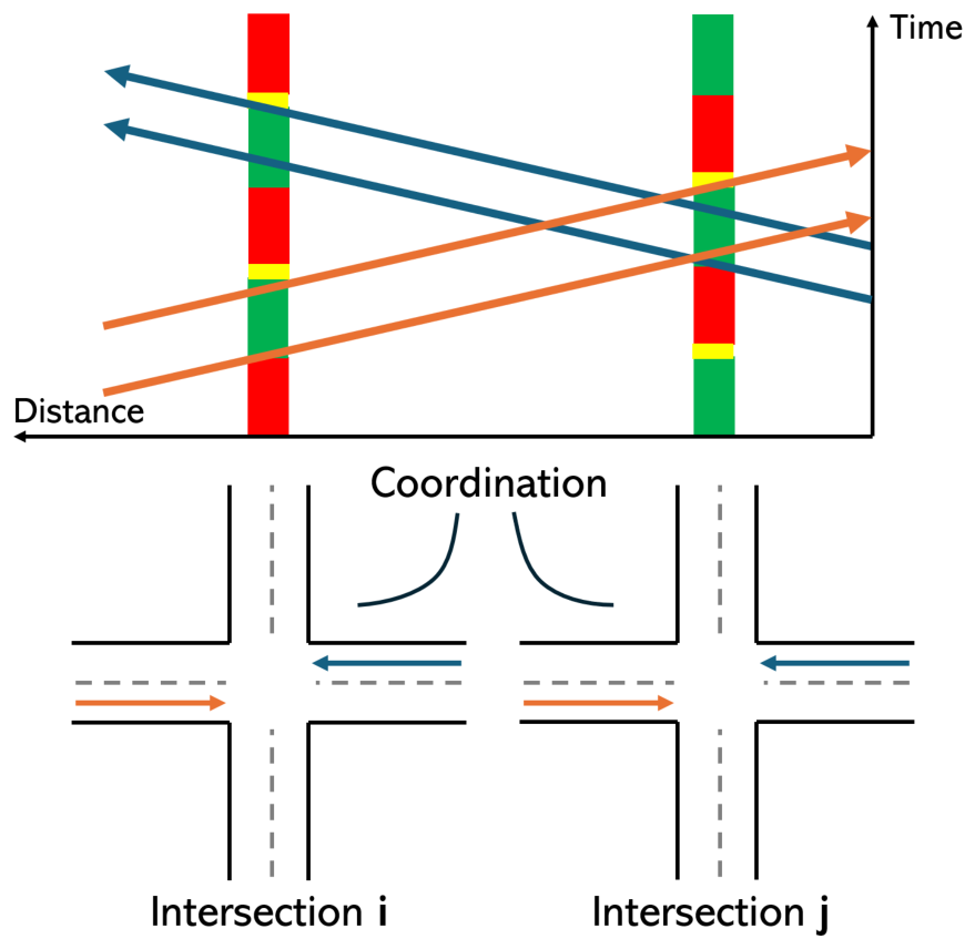
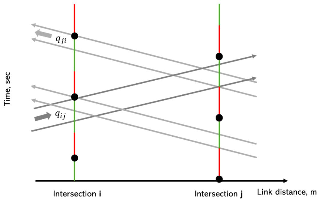
To make the SCN weight directly represent the operational value of coordination, we estimate the pairwise weight as the net hourly delay impact of coordinating two adjacent intersections. Specifically, for each adjacent pair $(i,j)$, we compare two timing plans. The first is a pairwise coordinated plan, where the two intersections operate under a common coordination cycle and the two opposing through directions are progressed using the calculated green bands. The second is an independent fixed-time plan, where the two intersections operate separately using their own locally preferred timing plans. As shown in Figure 1, signal coordination may reduce delay by creating green band time per unit time through coordination [38]. However, it may also introduce additional delay because the intersections need to match their timing plans, especially the cycle length [2,39]. Therefore, the SCN edge weight is defined as the difference between the total hourly delay in the independent case and that in the coordinated case.

For the coordinated case, the common cycle length is first determined from the locally preferred Webster cycle lengths. Let $C_i^0$ and $C_j^0$ denote the locally preferred cycle lengths of intersections i and j, respectively. Following the FHWA Signal Timing Manual, the common coordination cycle is selected as

$$C_{ij}=\max \left\{C_i^0,C_j^0\right\}.$$

(1)

Under this coordinated timing plan, $C_{ij}$ is the actual cycle length applied to both intersections. Therefore, all effective green times used in the coordinated case are recalculated under this common cycle. For movement m at intersection $r\in \{i,j\}$, the common-cycle green time is denoted by $g_{r,m}^{\left(ij\right)}$. The calculation follows the Webster-based split allocation:

$$g_{r,m}^{\left(ij\right)}={\displaystyle \frac{y_{r,m}}{Y_r}}\left(C_{ij}-L_r\right),$$

(2)

where $y_{r,m}$ is the critical flow ratio associated with movement m, $Y_r$ is the sum of critical flow ratios at intersection r, and $L_r$ is the total lost time per cycle. This notation clarifies that the green time used for coordinated evaluation is based on the actual common cycle, rather than on two separate local cycles.

The two coordinated through directions are $i\to j$ and $j\to i$. Their directional green bands, denoted by $B_{ij}^{\ast }$ and $B_{ji}^{\ast }$, are calculated using the pairwise two-way bandwidth procedure described in Appendix A.2. This procedure accounts for intersection spacing, progression speed, common cycle length, and directional traffic demand through the directional travel times between the two intersections [40,41].

Next, we estimate the delay under the coordinated timing plan. For movement m at intersection r, let $q_{r,m}$ be the hourly traffic volume and $s_{r,m}$ be the saturation flow rate. The green ratio under the common-cycle timing plan is

$${\lambda }_{r,m}^{\left(ij\right)}={\displaystyle \frac{g_{r,m}^{\left(ij\right)}}{C_{ij}}}.$$

(3)

The corresponding degree of saturation is calculated as

$$X_{r,m}^{\left(ij\right)}={\displaystyle \frac{q_{r,m}}{s_{r,m}{\lambda }_{r,m}^{\left(ij\right)}}}.$$

(4)

The average uniform-arrival delay of movement m at intersection r under the common-cycle timing plan is estimated using the uniform delay component of signalized-intersection delay [42,43]:

$$d_{r,m}^{\mathrm{com}}={\displaystyle \frac{0.5C_{ij}{\left(1-{\lambda }_{r,m}^{\left(ij\right)}\right)}^2}{1-\min \left\{1,X_{r,m}^{\left(ij\right)}\right\}{\lambda }_{r,m}^{\left(ij\right)}}}.$$

(5)

Here, $d_{r,m}^{\mathrm{com}}$ is measured in seconds per vehicle. It represents the average control delay experienced by vehicles of movement m at intersection r when intersections i and j are forced to operate under the common coordination cycle. This analytical delay expression is used only to construct the SCN weights; the final traffic performance is still evaluated through SUMO simulation.

Before applying the progression saving, the total hourly delay of the two intersections under the common-cycle timing plan is calculated as

$$D_{ij}^{\mathrm{com}}=\sum _{r\in \{i,j\}}\sum _{m\in {\mathcal{M}}_r}{q}_{r,m}{d}_{r,m}^{\mathrm{com}}.$$

(6)

This equation has a direct physical meaning: for each movement, the hourly traffic volume is multiplied by the average delay per vehicle, and the results are summed over all movements at the two intersections. Therefore, $D_{ij}^{\mathrm{com}}$ includes through movements, turning movements, and side-street movements, and captures the possible delay increase caused by forcing the two intersections to operate under a common cycle.

The calculated directional green bands reduce the downstream delay of the two coordinated through movements. For the $i\to j$ direction, the number of vehicles per hour that can be accommodated by the green band is estimated as

$$Q_{ij}^{\mathrm{pass}}=\min \left\{q_{ij},{\overline{s}}_{ij}{\displaystyle \frac{B_{ij}^{\ast }}{C_{ij}}}\right\},{\overline{s}}_{ij}=\min \left\{s_i^{ij},s_j^{ij}\right\}.$$

(7)

Here, $q_{ij}$ is the directional through volume from i to j, and $s_i^{ij}$ and $s_j^{ij}$ are the corresponding through-movement saturation flow rates at intersections i and j. The same calculation is applied to the reverse direction.

The hourly saving from progression is estimated only for the two coordinated through directions. Let $d_{ij}^{\mathrm{down}}$ denote the average downstream delay per vehicle for vehicles traveling from i to j under the common-cycle timing plan. Similarly, let $d_{ji}^{\mathrm{down}}$ denote the average downstream delay per vehicle for vehicles traveling from j to i. These delay values are obtained from the corresponding downstream through movements using the uniform-delay calculation defined above.

The hourly progression saving is calculated as

$$S_{ij}^{\mathrm{save}}=Q_{ij}^{\mathrm{pass}}{d}_{ij}^{\mathrm{down}}+Q_{ji}^{\mathrm{pass}}{d}_{ji}^{\mathrm{down}}.$$

(8)

This equation means that the number of vehicles passing through the green band is multiplied by the downstream delay avoided per vehicle. The first term represents the saving for the $i\to j$ direction, while the second term represents the saving for the $j\to i$ direction. Other movements are not assigned a direct green-band saving, but their delays are still included in the common-cycle delay term $D_{ij}^{\mathrm{com}}$.

Therefore, the total hourly delay under pairwise coordination is estimated as

$$D_{ij}^{\mathrm{coord}}=D_{ij}^{\mathrm{com}}-S_{ij}^{\mathrm{save}}.$$

(9)

For the independent fixed-time case, intersections i and j operate separately using their own locally preferred Webster cycle lengths and green splits. The average delay of each movement is calculated using the same uniform-delay expression, but with the local cycle length and local green time of that intersection. Let $d_{r,m}^0$ denote the average delay per vehicle of movement m at intersection r under this independent timing plan. The total hourly delay under independent operation is then

$$D_{ij}^{\mathrm{ind}}=\sum _{r\in \{i,j\}}\sum _{m\in {\mathcal{M}}_r}{q}_{r,m}{d}_{r,m}^0.$$

(10)

This term represents the total hourly delay when the two intersections keep their own locally preferred timing plans, without being forced into a common coordination cycle.

Finally, the SCN edge weight is defined as the net hourly delay reduction obtained by coordinating the two intersections:

$$w_{ij}=D_{ij}^{\mathrm{ind}}-D_{ij}^{\mathrm{coord}}.$$

(11)

A positive value of $w_{ij}$ indicates that coordination is expected to reduce total hourly delay for the pair $(i,j)$, while a negative value indicates that coordination may introduce extra delay compared with independent operation. Compared with the previous green-band-minus-penalty formulation, this revised weight directly measures the net operational value of coordination in vehicle-seconds saved per hour. The effect of cycle-length mismatch is captured by comparing the independent-delay term $D_{ij}^{\mathrm{ind}}$ with the common-cycle delay term $D_{ij}^{\mathrm{com}}$, rather than by adding a separate cycle-matching penalty. The effect of spacing and progression speed is captured through the calculated directional green bands.

3.2. Intersection Grouping via SCN Partitioning

Given the constructed SCN that preserves the pairwise coordination relationships between adjacent intersections, we further need to construct detailed intersection groups. These groups correspond to different signal control strategies among intersections. In this study, we classify them into three major categories: isolated signal timing, arterial progression, and network progression. Isolated signal timing represents intersections that do not participate in coordination, while arterial progression and network progression represent two different structures of signal coordination. Together, these three categories cover the timing strategy of the entire signalized network. In other words, the original network is partitioned into a set of intersection groups, and the objective is to identify the partitioning scheme that provides the maximum total coordination benefit.

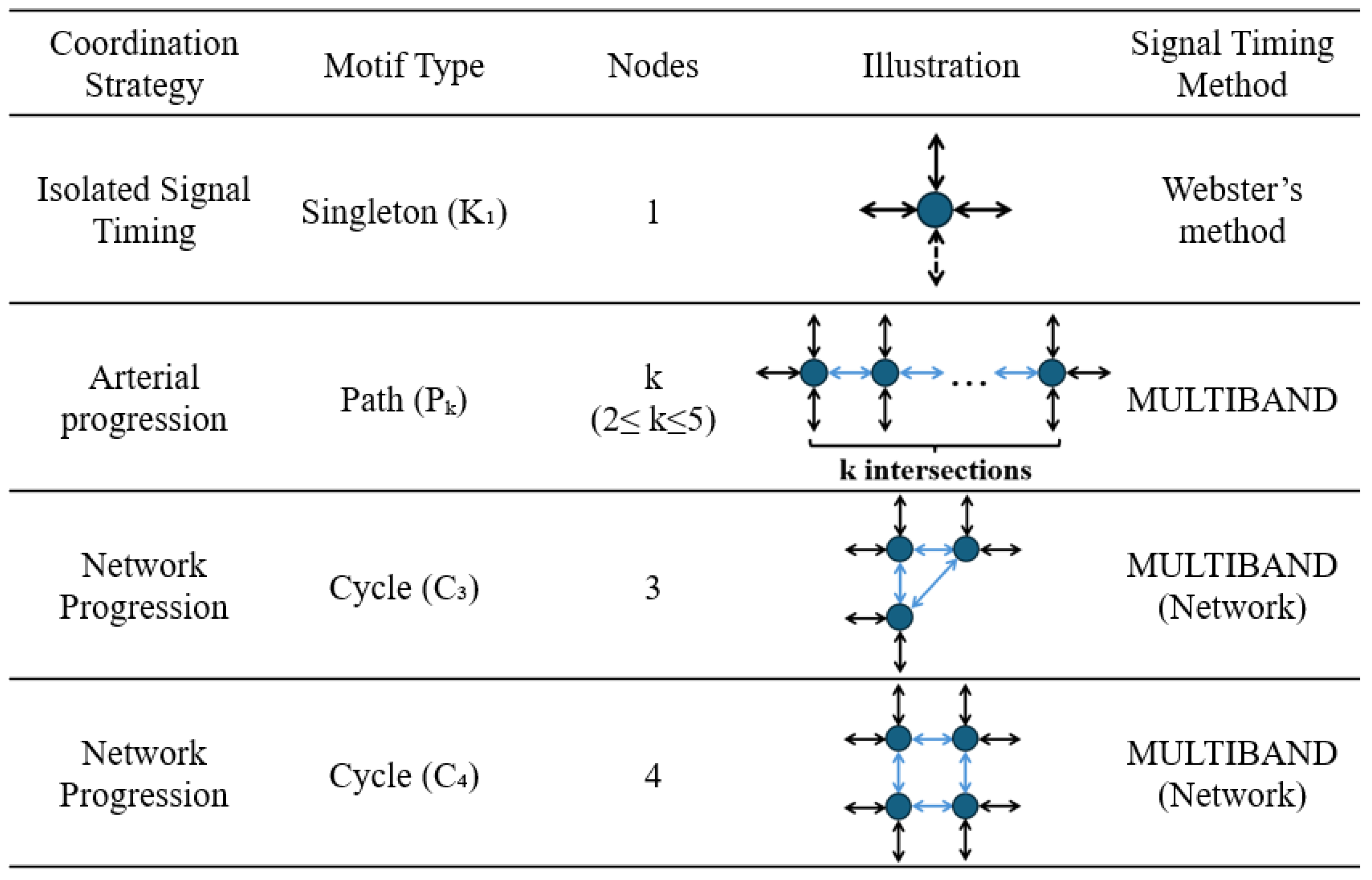
To define feasible intersection groups in a structured way, we use the concept of network motifs [44]. A motif is a small subgraph pattern that represents a basic and recurring local structure in a network. In this study, we define a coordination motif as a subgraph that corresponds to a feasible and practical signal control configuration. As shown in Figure 2, four motif types are considered:

• $K_1$: Singleton motifs, where an intersection operates independently using isolated signal timing.
• $P_k$: Linear path motifs with $2\le k\le 5$, representing arterial progression along a corridor.
• $C_3$: Three-node cycle motifs, representing a small loop structure for network progression.
• $C_4$: Four-node cycle motifs, representing a square-like grid structure for network progression.

Figure 2. Coordination strategies, motif types, and corresponding signal timing methods. Blue nodes represent intersections, arrows indicate traffic movements, and the ellipsis denotes intermediate intersections.

Figure 2. Coordination strategies, motif types, and corresponding signal timing methods. Blue nodes represent intersections, arrows indicate traffic movements, and the ellipsis denotes intermediate intersections.

For network progression, the cycle motifs $C_3$ and $C_4$ should be understood as basic building blocks rather than the only possible network-level intersection groups. In dense urban networks, a network progression group may contain multiple connected loop motifs. For example, several adjacent $C_4$ motifs can be combined to form a larger grid-based intersection group. Therefore, after identifying basic motifs from the SCN, compatible motifs of the same network-progression type can be merged to generate larger candidate intersection groups. The candidate motif set $\mathcal{Q}$ is generated by a simple enumeration procedure on the SCN. Since only short paths and small loops are considered, the enumeration step is efficient for the medium-scale urban networks considered. For loop motifs, an additional offset-consistency check is applied. A single offset variable $O_i$ is assigned to each intersection i in the loop. For each directed internal edge $(i,j)$, the offset relationship must be feasible under the common cycle

$$O_j-O_i\equiv {\theta }_{ij}\left(\mathrm{mod}{C}_q\right),$$

(12)

within the feasible green-band window. A loop motif is retained only if a consistent offset assignment exists for all internal edges. This avoids selecting loop motifs whose pairwise bandwidths cannot be realized simultaneously around the closed cycle.

In implementation, the candidate motif set is generated in three steps. First, singleton motifs are created for all signalized intersections so that every intersection can remain isolated if coordination is not beneficial. Second, path motifs are enumerated by starting from each intersection and expanding along adjacent SCN edges to form simple linear paths with $2\le k\le 5$ intersections. Only paths without repeated nodes are retained, and duplicated paths generated from different starting directions are removed. Third, loop-based motifs are enumerated by searching for simple three-node and four-node cycles in the SCN. These cycle motifs are used as basic network-progression units. After the basic motifs are generated, compatible loop motifs that share intersections or internal edges can be selected together and later merged into a larger network-progression group, while path motifs and singleton motifs remain mutually exclusive with any other motif sharing the same intersection.

Therefore, the intersection grouping problem is formulated as a maximum weighted set-packing problem over the candidate coordination motifs [45,46]. The objective is to select a subset of motifs that maximizes the total coordination benefit while ensuring that every signalized intersection is assigned to at least one feasible timing strategy. Since network progression groups may be formed by multiple connected loop motifs, compatible overlaps among loop-based motifs are allowed. However, incompatible overlaps are prohibited, and redundant benefits introduced by overlapping loop motifs are deducted from the objective function.

Let $\mathcal{Q}=\{1,2,\dots ,Q\}$ denote the set of candidate coordination motifs generated from the SCN. Each candidate motif $q\in \mathcal{Q}$ is associated with a node set ${\mathcal{V}}_q\subseteq \mathcal{V}$, an internal edge set ${\mathcal{E}}_q\subseteq \mathcal{E}$, and a motif type $m_q$. The benefit of motif q is defined as the sum of pairwise SCN weights over its internal edges:

$$W_q=\sum _{(i,j)\in {\mathcal{E}}_q}{w}_{ij},$$

(13)

where $w_{ij}$ is the SCN edge weight defined in Equation (11). For a singleton motif $K_1$, the internal edge set is empty and its benefit is set to zero. Equation (13) approximates the group-level coordination benefit by aggregating pairwise coordination potentials. As each $w_{ij}$ is evaluated using the common cycle associated with intersection pair $(i,j)$, the edge weights are not recomputed under a unified cycle for the entire motif. This additive formulation is adopted to simplify benefit evaluation and preserve the computational tractability of the subsequent partitioning optimization. We note that, when the internal edges favor different cycle lengths, this approximation may overestimate the coordination benefit of larger motifs.

The binary decision variable $x_q$ indicates whether motif q is selected:

$$x_q=\left\{\begin{array}{cc}1,\hfill & \mathrm{if}\mathrm{motif}q\mathrm{is}\mathrm{selected},\hfill \\ 0,\hfill & \mathrm{otherwise}.\hfill \end{array}\right.$$

The motif-based set-packing problem [47,48] is formulated as:

$$\begin{array}{c}\underset{\mathbf{x}}{\max }\sum _{q\in \mathcal{Q}}{W}_q{x}_q-\sum _{\begin{array}{c}q,r\in \mathcal{Q}\\ q<r\end{array}}{\Delta }_{qr}{x}_q{x}_r\hfill \\ \mathrm{s}.\mathrm{t}.\sum _{q\in \mathcal{Q}:v\in {\mathcal{V}}_q}{x}_q\ge 1,\forall v\in \mathcal{V},\hfill \\ x_q+x_r\le 1,\forall q<r:{\mathcal{V}}_q\cap {\mathcal{V}}_r\ne \varnothing ,\{m_q,m_r\}⊈{\mathcal{M}}_{\mathrm{loop}},\\ x_q\in \{0,1\},\forall q\in \mathcal{Q}.\hfill \end{array}$$

(14)

where ${\mathcal{M}}_{\mathrm{loop}}=\{C_3,C_4\}$ is the set of loop-based motif types. The term ${\Delta }_{qr}$ denotes the redundant coordination benefit that would be double-counted when two compatible loop motifs q and r overlap. It is calculated based on their shared internal SCN edges:

$${\Delta }_{qr}=\sum _{(i,j)\in {\mathcal{E}}_q\cap {\mathcal{E}}_r}{w}_{ij}.$$

(15)

If two selected loop motifs share no internal edge, then ${\Delta }_{qr}=0$.

Remark 1.

Equation (14) can be interpreted as a generalized exact-cover formulation. At the grouping level, each intersection should belong to one final intersection group and receive exactly one corresponding timing strategy. Note that the optimization is performed over basic coordination motifs rather than final groups. Therefore, compatible loop motifs are allowed to overlap during motif selection, so that multiple motifs can be combined into a larger network progression group. The quadratic penalty term corrects the duplicated benefit from shared internal edges.

The objective function maximizes the total benefit of selected motifs while deducting redundant benefits caused by overlapping loop motifs. The first constraint requires every intersection to be covered by at least one selected motif, ensuring that each signalized intersection receives a timing strategy. The second constraint prohibits incompatible overlaps. Specifically, if two motifs share nodes but are not both loop-based motifs, they cannot be selected simultaneously. The last constraint defines the binary selection decision.

The optimization problem is solved as a mixed-integer quadratic programming problem using CPLEX. After the binary variables are optimized, all selected singleton motifs are directly treated as isolated intersections, selected path motifs are treated as arterial progression groups, and connected selected loop motifs are merged into network-progression groups. The final output is therefore a partition of the signalized network into isolated, arterial, and network-progression intersection groups. This output is then passed to the corresponding timing optimization method summarized in Figure 2.

4. Experiments

This section evaluates the proposed SCN-based intersection grouping framework under different network layouts and ToD demand scenarios. The experiments are designed to answer three questions: (1) whether the proposed method can generate reasonable intersection groups under different traffic demand patterns; (2) whether the selected groups improve network-level traffic performance compared with fixed, adaptive, corridor-based, and network-wide coordination strategies; and (3) whether selective coordination is more effective than applying coordination uniformly to predefined corridors or to the entire network.

4.1. Experiment Settings

The experiments were conducted using the Simulation of Urban Mobility (SUMO), a widely used open-source traffic simulation platform capable of modeling vehicular dynamics and traffic signal operations [49]. For the signal coordination and the timing plans, MAXBAND/MULTIBAND optimization was implemented externally in Python 3.12, where the common cycle length, phase durations, progression bandwidths, and intersection offsets were calculated through mathematical optimization. The optimized timing parameters were then converted into SUMO-compatible signal programs. The motif-based grouping problem was implemented in Python. Network construction and motif enumeration were conducted using graph-based enumeration procedures, and the resulting MIQP problem was solved using CPLEX [50].

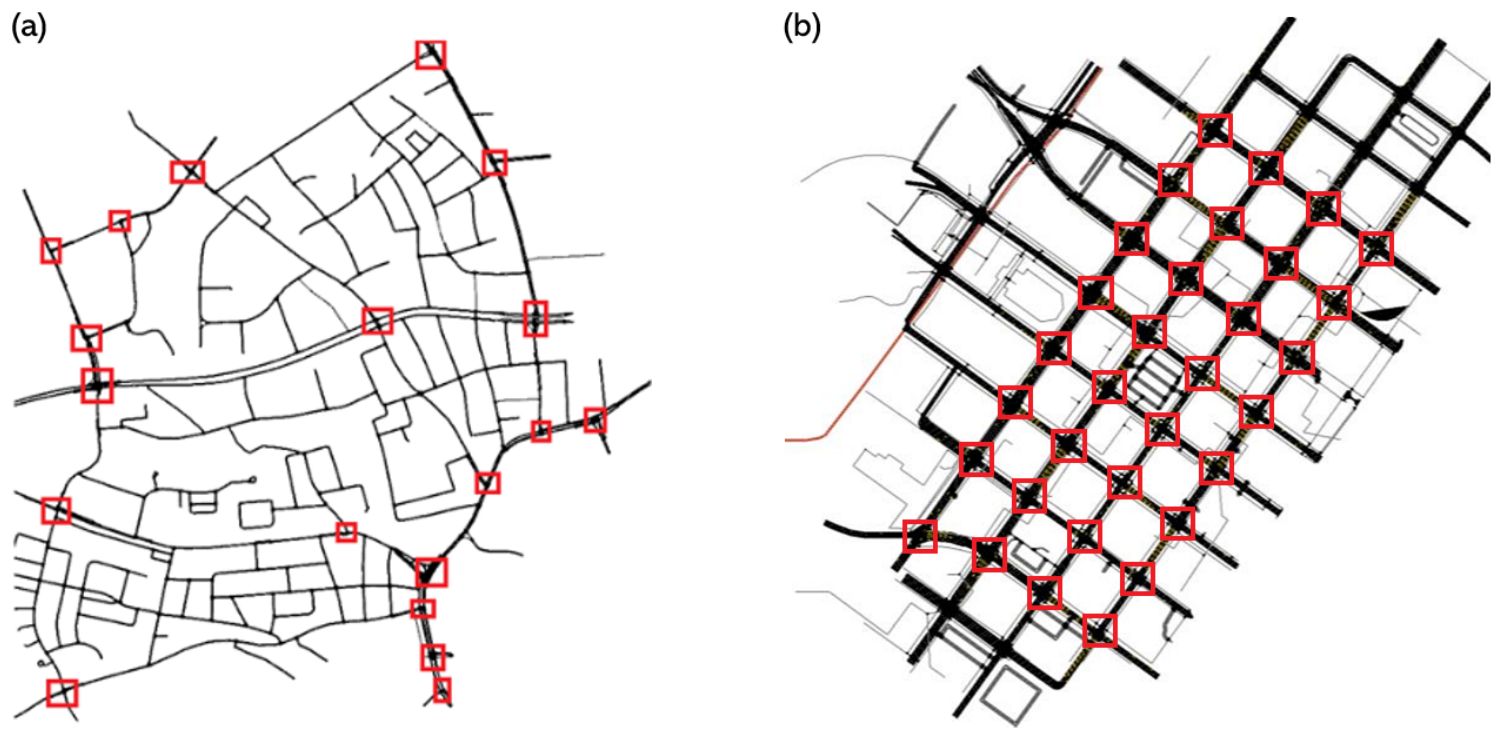
Two urban networks were used in the experiments. The first network is an open-source traffic network from Ingolstadt, Germany, as shown in Figure 3a. The second network is a constructed urban network representing downtown Houston, United States, as shown in Figure 3b. These two networks provide different roadway structures and demand patterns, allowing the proposed method to be tested under heterogeneous urban settings. The Ingolstadt, Germany, network covers the Nordwest Stadtbezirk and adjacent downtown blocks, including 21 signalized intersections. This network represents a typical European urban network with irregular geometry and varying intersection spacing. The traffic demand profiles were obtained from the open-source SUMO network data and represent hourly demand variations under realistic traffic conditions [51,52]. The downtown Houston network was constructed with 32 signalized intersections. The network reflects a more regular urban grid structure. Traffic demands were estimated from local loop detector volumes and adjusted using annual average daily traffic (AADT) information to represent realistic hourly traffic fluctuations in the central business district [53].

To evaluate the effectiveness of the proposed coordination strategy under varying traffic conditions, four ToD scenarios were considered. The morning peak period represents high inbound traffic demand during 6:00–9:00. The midday period represents moderate traffic demand during 10:00–14:00. The evening peak period represents high outbound traffic demand during 15:00–18:00. The off-peak period represents low traffic demand during 19:00–5:00. For each network and ToD scenario, traffic volumes were assigned to the corresponding OD or directional demand profiles before running the simulation.

4.2. Baseline Strategies and Evaluation Metrics

The proposed method is compared with seven baseline signal timing strategies. Since there is no directly comparable network partitioning baseline for signal coordination group selection, the baselines are designed to represent commonly used or practically meaningful coordination choices. They also serve as an ablation-style comparison because each baseline emphasizes a different coordination assumption. Detailed implementation settings are provided in Appendix B, and the baseline descriptions are summarized as follows:

• Base Signal Timing Plan. For the Ingolstadt, Germany, network, the original network data provide a base signal timing plan, which is used as the baseline without adaptive control or signal coordination. For the Houston network, the base fixed-time signal plan is generated based on AADT values and hourly demand factors, and the cycle length is calculated using Webster’s method.
• Base Adaptive Signal Timing Plan. For the Ingolstadt network, nine intersections are configured with predefined minimum and maximum green durations and are operated as actuated intersections in SUMO. For the Houston network, the major east–west movements are set as actuated movements. Following the Traffic Signal Timing Manual [35], the minimum and maximum green durations are set within 5–10 s and 25–50 s, respectively, depending on the intersection demand.
• Optimized Fixed-Time Plan. Based on hourly demand and hourly demand factors, an optimized fixed-time signal timing plan is generated for each hourly demand period and applied to both networks. No adaptive control or signal coordination is applied in this baseline.
• Optimized Adaptive Signal Timing Plan. Based on the optimized fixed-time plan, actuated control is further applied to the major movements at intersections. This baseline is used to evaluate the performance of SUMO actuated control when combined with optimized fixed-time signal parameters.
• Major Corridor MAXBAND. The MAXBAND algorithm is applied to the major corridors to generate corridor-based signal coordination plans.
• Major Corridor MULTIBAND. The MULTIBAND algorithm is applied to the major corridors to generate corridor-based signal coordination plans with directional bandwidth consideration.
• Network MULTIBAND. The MULTIBAND algorithm is further applied at the selected network blocks. For the Houston network, the whole regional network is considered for network-level coordination.
• Proposed Method. Depending on traffic demand and network structure, the proposed method partitions the network into coordination regions and applies the corresponding coordination strategy to each region.

Traffic performance is evaluated using two metrics: average travel time per vehicle and average delay per vehicle. Average travel time measures the total time required for vehicles to complete their trips, while average delay measures the additional time caused by signal control, queuing, interruptions, and other operational constraints relative to expected movement conditions [18].

4.3. Results and Discussion

This subsection presents the intersection grouping results and evaluates their impacts on traffic operations. The main purpose of the experiments is not only to test whether signal coordination improves traffic performance, but also to examine whether the proposed SCN-based method can identify where coordination should and should not be applied.

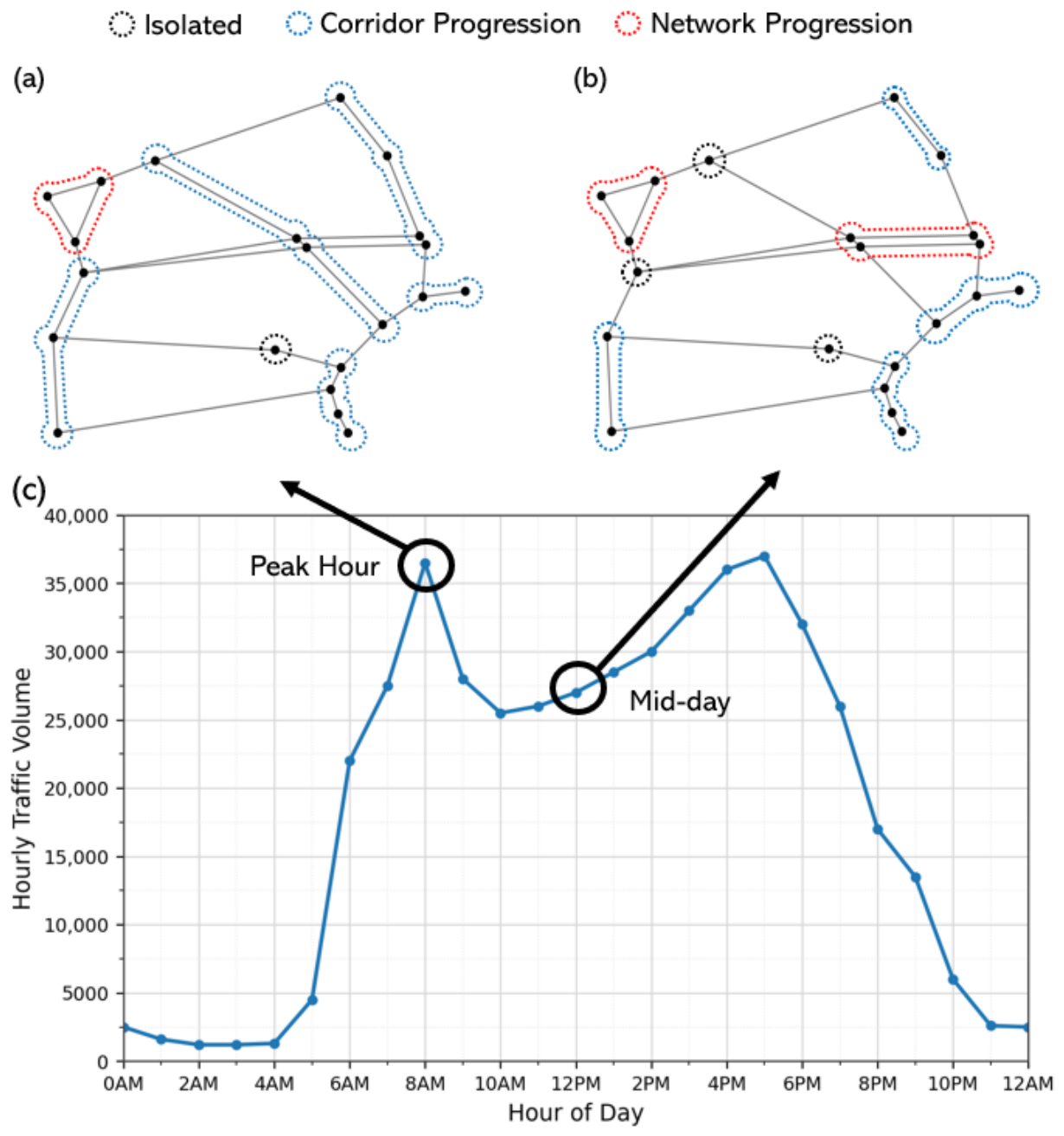
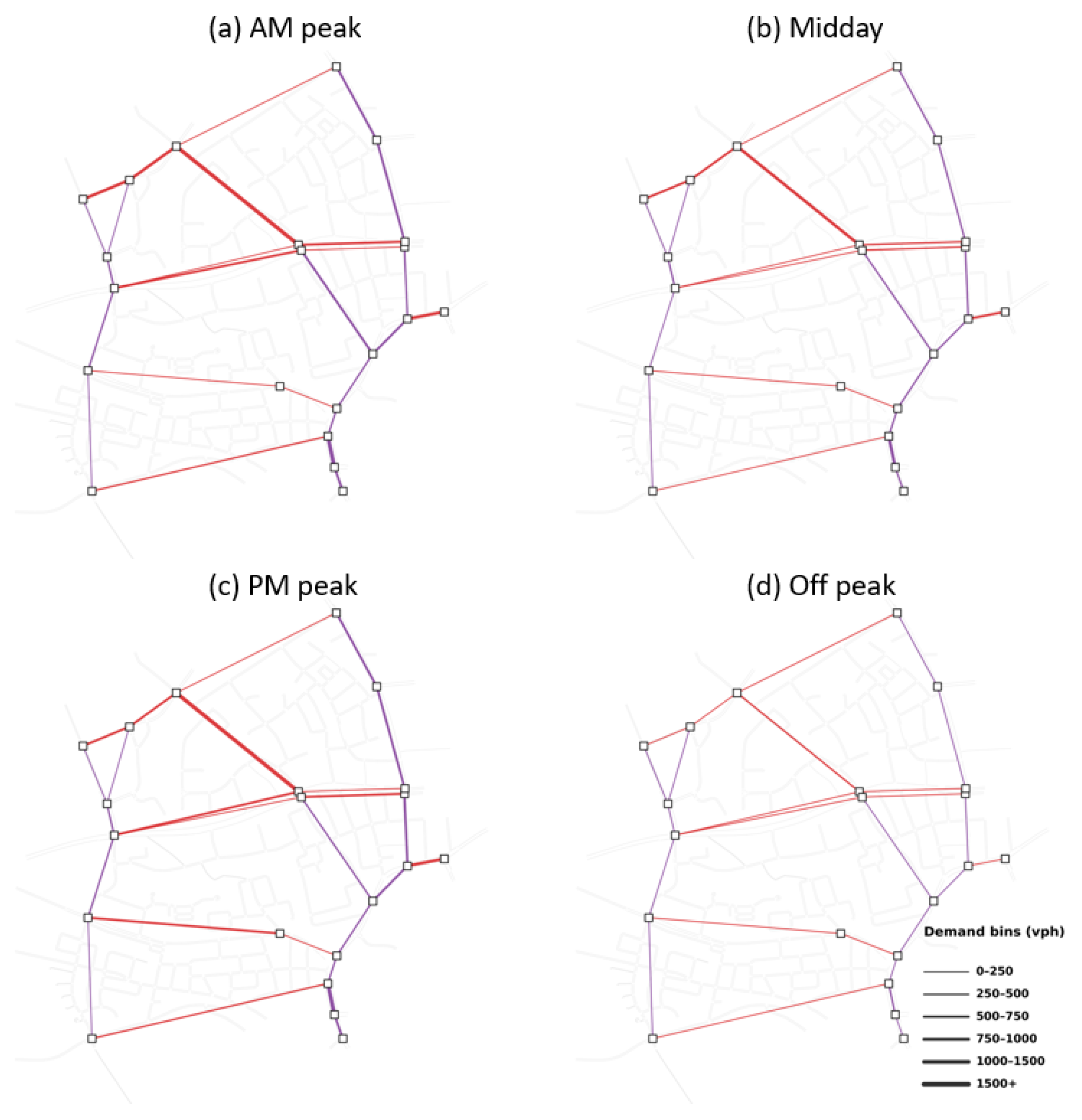
Figure 4 illustrates the partitioning results for the Ingolstadt network under peak-hour and off-peak conditions. The proposed method generates different intersection groups under different demand patterns. During peak hours, more intersections are grouped into arterial or network progression regions, especially in the central part of the network where intersections are spatially close and traffic demand is more concentrated. In contrast, during off-peak periods, several intersections are assigned to isolated timing. This occurs because the potential green-band benefit becomes smaller when demand is low, while forcing intersections to share a compatible cycle length may still introduce unnecessary timing constraints. It reflects the trade-off between progression benefit and cycle-matching cost.

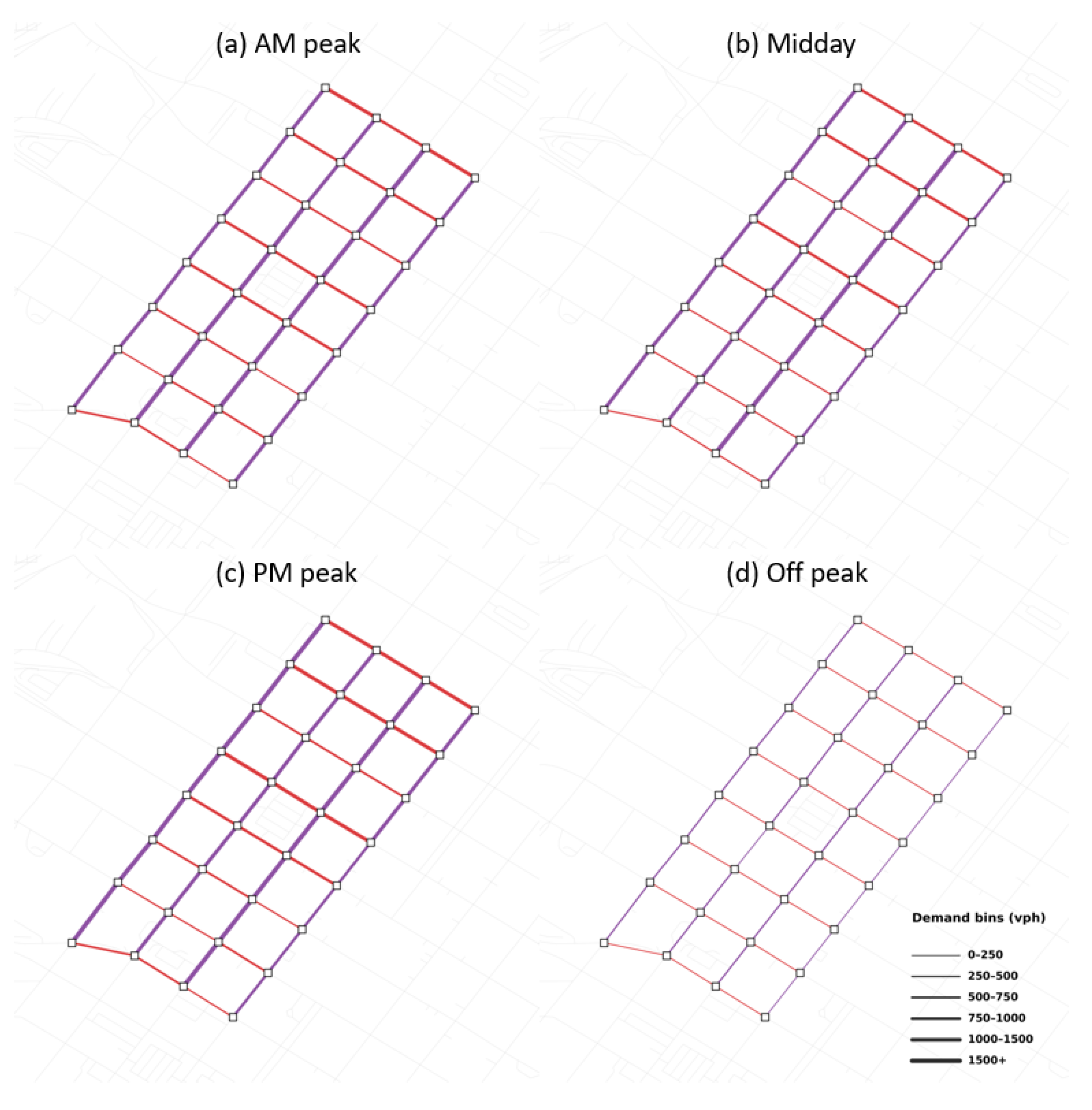
Furthermore, Figure 5 presents the demand patterns and the corresponding partitioning results for the Houston network. Compared with the Ingolstadt network, the Houston test network has a more regular grid structure. Therefore, when the traffic demand is relatively balanced, the proposed method tends to identify larger connected progression blocks. For example, during the off-peak period, the whole 32-intersection grid can be coordinated as a regional network-progression block. During peak periods, however, the demand becomes more concentrated along several directional arterials, especially the northbound and southbound movements. This directional imbalance reduces the benefit of coordinating the entire grid under one common progression structure. As a result, the proposed method partitions the network into smaller corridor- or block-level intersection groups.

This result highlights the main advantage of the proposed method: signal coordination is not treated as a uniform network-wide decision. Instead, the SCN weights allow the algorithm to distinguish intersections that are suitable for coordination from those where coordination is likely to provide limited or even negative benefit. Intersections that are far apart, weakly connected, or associated with incompatible timing requirements tend to remain isolated. By contrast, intersections with strong pairwise coordination benefits are selected into arterial or network progression groups. As a result, the proposed method provides a demand-sensitive and topology-aware way to determine intersection groups, rather than relying on fixed corridors or manually predefined control regions.

Table 1. Average Vehicle Travel Time (s/veh) by Signal Timing Strategy and Time-of-Day Scenario.

Signal Timing Strategy	Ingolstadt				Houston
	AM	Midday	PM	Off	AM	Midday	PM	Off
Base Timing Plan	290.1	252.6	295.9	231.0	126.3	126.2	126.7	125.2
Base Adaptive Timing Plan	257.7	233.3	253.1	218.1	71.7	79.1	70.4	73.9
Optimized Fixed-Time Plan	266.3	229.5	260.3	210.7	109.4	101.0	106.2	115.0
Optimized Adaptive Timing Plan	242.8	225.3	236.9	206.4	65.5	66.5	66.8	70.2
Major Corridor MAXBAND	264.2	228.8	280.0	213.6	115.9	116.4	117.2	116.7
Major Corridor MULTIBAND	249.5	221.4	245.3	205.6	88.0	88.3	117.6	111.3
Network MULTIBAND	233.6	202.4	227.7	190.7	64.1	60.9	62.6	58.3
Proposed Coordination Plan	217.8	201.6	218.8	189.1	60.9	60.0	61.3	58.3

Note: Bold values indicate the best performance in each scenario. Tied best values are both shown in bold.

and 

Table 2. Average Vehicle Delay (s/veh) by Signal Timing Strategy and Time-of-Day Scenario.

Signal Timing Strategy	Ingolstadt				Houston
	AM	Midday	PM	Off	AM	Midday	PM	Off
Base Timing Plan	144.9	108.7	150.5	88.2	87.7	87.6	88.0	86.7
Base Adaptive Timing Plan	113.4	90.1	109.1	75.6	33.1	40.5	31.7	35.4
Optimized Fixed-Time Plan	121.1	86.3	116.3	68.3	70.8	62.5	67.5	76.4
Optimized Adaptive Timing Plan	98.7	82.3	93.2	63.8	26.9	27.9	28.2	31.6
Major Corridor MAXBAND	120.0	85.8	134.7	71.2	77.3	77.9	78.5	78.1
Major Corridor MULTIBAND	105.9	78.5	102.0	63.2	49.4	49.7	79.0	72.7
Network MULTIBAND	89.6	59.7	84.1	48.1	25.5	22.3	23.9	20.5
Proposed Coordination Plan	74.7	58.8	75.8	46.6	22.3	21.4	22.7	20.5

Note: Bold values indicate the best performance in each scenario. Tied best values are both shown in bold.

summarize the comparison across both networks and all ToD scenarios. Among the eight network–ToD scenarios, the proposed partition-based timing outperforms all non-proposed baselines in seven of the eight scenarios in terms of both average travel time and delay. Compared with the best-performing non-proposed baseline in each scenario, it reduces average travel time by 2.7% and average delay by 7.0% across the tested scenarios. The improvements are particularly evident in the peak-period Ingolstadt cases, indicating that the identified intersection groups provide a more effective coordination structure than the predefined corridor- and network-level alternatives. In the Houston off-peak case, the proposed method recommends full-network coordination, as shown in Figure 5, and therefore produces the same reported performance as Network MULTIBAND. These results demonstrate that the proposed framework can identify coordination structures suited to the two networks under different demand conditions while delivering improved performance in most scenarios.

The comparison with corridor-based methods provides a useful interpretation. Major Corridor Maxband and Major Corridor Multiband generally outperform the fixed-time uncoordinated plan, confirming that arterial progression is effective when the selected corridor is suitable for coordination. However, their performance is limited by the predefined corridor structure. They cannot fully adapt when demand shifts across different parts of the network, and they may miss locally important coordination opportunities outside the selected arterial. The proposed method addresses this limitation by allowing different coordination structures to coexist. Some intersections remain isolated, some are grouped into corridors, and others are assigned to network progression regions. This flexibility explains why the proposed method performs better than corridor-only coordination in both networks.

The comparison with the network progression baseline shows why full network-wide coordination is not always desirable. Network progression can improve traffic performance when intersections are dense and timing requirements are compatible. However, applying it too broadly may force intersections with different demand patterns into a common coordination structure. This can reduce the benefit of progression and increase delay for movements that are not aligned with the dominant coordinated flows. In the experiments, the network progression baseline does not consistently outperform the corridor-based methods, especially in the Ingolstadt network. This suggests that coordination should be spatially selective rather than uniformly imposed on the entire network.

To further examine the robustness and performance of the proposed method, we conducted sensitivity analyses for both the selected intersection groups and the SUMO simulation results, as detailed in Appendix B.3. For model performance, the within-run bootstrap analysis and the additional stochastic demand-variation experiment show that the proposed method generally achieves the lowest or near-lowest mean travel time and delay across the evaluated scenarios. Its advantage over the strongest network-level progression baseline nevertheless remains relatively small in several low-demand cases. For network partitioning, the selected groups are generally stable under moderate demand and edge-weight perturbations, while still adapting to changes in the relative coordination benefits. However, greater sensitivity is observed in some PM peak scenarios, particularly for the Houston network under random edge-weight perturbations. These results indicate that the framework is robust in most tested conditions, while partition stability should be interpreted with additional care under highly congested or rapidly changing traffic conditions.

Overall, the experiments demonstrate that the proposed method improves traffic performance by coordinating only where coordination is beneficial. Fixed-time control ignores coordination opportunities, corridor-based methods depend on predefined arterial structures, and full network progression may over-coordinate intersections with incompatible timing needs. In contrast, the proposed SCN partitioning method selects intersection groups based on the estimated net benefit of coordination, considering both green-band opportunities and cycle-matching drawbacks. This produces a more balanced timing structure and leads to improved or comparable performance across the tested network layouts and ToD demand conditions.

5. Conclusions and Future Work

This study proposed a novel network partitioning approach for identifying effective traffic signal intersection groups under different time-of-day demand conditions. Instead of assuming that intersection groups are predefined, the proposed framework explicitly models group selection as a network-level optimization problem. An SCN was constructed to quantify the potential coordination benefit between adjacent intersections by considering traffic demand, spatial proximity, and cycle-length compatibility. Candidate coordination motifs were then generated to represent isolated intersections, arterial progression groups, and network progression groups, and a maximum weighted set-packing problem was formulated to select the intersection groups with the highest overall benefit. Experiments on the Ingolstadt and Houston networks show that the proposed partition-based timing strategy achieves the lowest mean travel time and delay in seven of the eight evaluated demand scenarios compared with carefully selected baselines, while performing comparably to the best baseline in the remaining scenario. These results demonstrate that effective signal coordination depends not only on optimizing timing plans within a given group, but also on selecting which intersections should be coordinated together. As the proposed pipeline performs well in SUMO simulations, potential sim-to-real discrepancies should be carefully considered in practical deployment. Meanwhile, the results on the two medium-scale networks provide useful evidence regarding scalability, while applications to other networks involve additional considerations.

Future work can extend the proposed framework in two directions. First, the current SCN construction approximates the benefit of a multi-intersection group by additively aggregating pairwise coordination relationships. This approximation simplifies benefit evaluation and preserves the computational tractability of the network partitioning problem. However, because each pairwise edge weight is evaluated using the common cycle identified for that intersection pair, the resulting motif benefit does not fully account for the unified cycle and mutually consistent offsets required by the entire group. Consequently, the additive formulation may overestimate the benefit of larger motifs when their internal edges favor different cycle lengths or offset patterns. Although the offset-closure condition introduced for loop motifs such as $C_3$ and $C_4$ improves group-level feasibility, it does not eliminate the approximation in the benefit calculation. Future studies could address this limitation by jointly determining group-level cycles and offsets, recomputing the corresponding delay-based benefits, incorporating higher-order coordination interactions, or adopting a hypergraph-based formulation. Second, learning-based methods can be explored for dynamic intersection group selection. With simulation environments such as SUMO, reinforcement learning could be used to learn when and where intersections should be coordinated based on traffic states, queue evolution, and progression quality, allowing the framework to move beyond time-of-day planning toward adaptive coordination strategies.

References

1. Papageorgiou, M.; Diakaki, C.; Dinopoulou, V.; Kotsialos, A.; Wang, Y. Review of road traffic control strategies. Proc. IEEE 2003, 91, 2043–2067. [Google Scholar] [CrossRef]
2. Little, J.D.C.; Kelson, M.D.; Gartner, N.H. MAXBAND: A versatile program for setting signals on arteries and triangular networks. Transp. Res. Rec. 1981, 795, 40–46. [Google Scholar]
3. Stamatiadis, C.; Gartner, N.H. MULTIBAND-96: A program for variable-bandwidth progression optimization of multiarterial traffic networks. Transp. Res. Rec. 1996, 1554, 9–17. [Google Scholar] [CrossRef]
4. Stevanovic, A. Adaptive Traffic Control Systems: Domestic and Foreign State of Practice; NCHRP Synthesis 403; Transportation Research Board: Washington, DC, USA, 2010. [Google Scholar]
5. Wong, S.C. Group-based optimisation of signal timings using the TRANSYT traffic model. Transp. Res. Part B Methodol. 1996, 30, 217–244. [Google Scholar] [CrossRef]
6. Zhang, L.; Song, Z.; Tang, X.; Wang, D. Signal coordination models for long arterials and grid networks. Transp. Res. Part C Emerg. Technol. 2016, 71, 215–230. [Google Scholar] [CrossRef]
7. Wen, X.; Wang, D.; Jin, S.; Qian, G.; Zhu, Y. A signal coordination model for long arterials considering link traffic flow characteristics. Sustainability 2023, 15, 14874. [Google Scholar] [CrossRef]
8. Ke, S.; Wang, Y.; An, C.; Lu, Z.; Xia, J. Traffic origin-destination flow-inspired dynamic urban arterial partition for coordinated signal control using automatic license plate recognition data. IEEE Intell. Transp. Syst. Mag. 2023, 16, 132–147. [Google Scholar] [CrossRef]
9. Roess, R.P.; Prassas, E.S.; McShane, W.R. Traffic Engineering, 4th ed.; Pearson Education: Upper Saddle River, NJ, USA, 2011. [Google Scholar]
10. Alshabibi, N.M. Comparing the saturation flow rate on the exit lane between urban multilane roundabouts and urban signalized intersections through field data. Infrastructures 2025, 10, 15. [Google Scholar] [CrossRef]
11. Abduljabbar, R.; Dia, H.; Liyanage, S. Machine learning traffic flow prediction models for smart and sustainable traffic management. Infrastructures 2025, 10, 155. [Google Scholar] [CrossRef]
12. Venglar, S.P.; Koonce, P.; Urbanik, T., II. PASSER TM III-98 Application and User’s Guide; Texas Transportation Institute, Texas A&M University: College Station, TX, USA, 1998. [Google Scholar]
13. An, K.; Chiu, Y.-C.; Hu, X.; Chen, X. A network partitioning algorithmic approach for macroscopic fundamental diagram-based hierarchical traffic network management. IEEE Trans. Intell. Transp. Syst. 2018, 19, 1130–1139. [Google Scholar] [CrossRef]
14. Saeedmanesh, M.; Geroliminis, N. Clustering of heterogeneous networks with directional flows based on “Snake” similarities. Transp. Res. Part B Methodol. 2016, 91, 250–269. [Google Scholar] [CrossRef]
15. Ji, K.; Tang, J.; Li, M.; Hu, C. Distributed traffic control based on road network partitioning using normalization algorithm. Sustainability 2023, 15, 11378. [Google Scholar] [CrossRef]
16. Michailidis, P.; Michailidis, I.; Lazaridis, C.R.; Kosmatopoulos, E. Traffic signal control via reinforcement learning: A review on applications and innovations. Infrastructures 2025, 10, 114. [Google Scholar] [CrossRef]
17. Wei, H.; Zheng, G.; Yao, H.; Li, Z. IntelliLight: A reinforcement learning approach for intelligent traffic light control. In Proceedings of the 24th ACM SIGKDD International Conference on Knowledge Discovery & Data Mining, London, UK, 19–23 August 2018; pp. 2496–2505. [Google Scholar] [CrossRef]
18. Wei, H.; Chen, C.; Zheng, G.; Wu, K.; Gayah, V.; Xu, K.; Li, Z. PressLight: Learning max pressure control to coordinate traffic signals in arterial network. In Proceedings of the 25th ACM SIGKDD International Conference on Knowledge Discovery & Data Mining, Anchorage, AK, USA, 4–8 August 2019; pp. 1290–1298. [Google Scholar] [CrossRef]
19. Wei, H.; Xu, N.; Zhang, H.; Zheng, G.; Zang, X.; Chen, C.; Zhang, W.; Zhu, Y.; Xu, K.; Li, Z. CoLight: Learning network-level cooperation for traffic signal control. In Proceedings of the 28th ACM International Conference on Information and Knowledge Management, Beijing, China, 3–7 November 2019; pp. 1913–1922. [Google Scholar] [CrossRef]
20. Fang, J.; You, Y.; Xu, M.; Wang, J.; Cai, S. Multi-objective traffic signal control using network-wide agent coordinated reinforcement learning. Expert Syst. Appl. 2023, 229, 120535. [Google Scholar] [CrossRef]
21. Borges, F.S.P.; Fonseca, A.P.; Garcia, R.C. Deep reinforcement learning model to mitigate congestion in real-time traffic light networks. Infrastructures 2021, 6, 138. [Google Scholar] [CrossRef]
22. Afshari, A.; Lee, J.; Besenski, D. A digital twin platform for real-time intersection traffic monitoring, performance evaluation, and calibration. Infrastructures 2025, 10, 204. [Google Scholar] [CrossRef]
23. Etemadnia, H.; Abdelghany, K.; Hassan, A. A network partitioning methodology for distributed traffic management applications. Transp. A Transp. Sci. 2014, 10, 518–532. [Google Scholar] [CrossRef]
24. Hunt, P.B.; Robertson, D.I.; Bretherton, R.D.; Winton, R.I. SCOOT: A Traffic Responsive Method of Coordinating Signals; Laboratory Report 1014; Transport and Road Research Laboratory: Crowthorne, UK, 1981. [Google Scholar]
25. Lowrie, P.R. SCATS, Sydney Co-Ordinated Adaptive Traffic System: A Traffic Responsive Method of Controlling Urban Traffic; Roads and Traffic Authority of New South Wales, Traffic Control Section: Darlinghurst, Australia, 1990. [Google Scholar]
26. Mirchandani, P.; Head, L. A real-time traffic signal control system: Architecture, algorithms, and analysis. Transp. Res. Part C Emerg. Technol. 2001, 9, 415–432. [Google Scholar] [CrossRef]
27. Yau, K.-L.A.; Qadir, J.; Khoo, H.L.; Ling, M.H.; Komisarczuk, P. A survey on reinforcement learning models and algorithms for traffic signal control. ACM Comput. Surv. 2017, 50, 3068287. [Google Scholar] [CrossRef]
28. Noaeen, M.; Naik, A.; Goodman, L.; Crebo, J.; Abrar, T.; Abad, Z.S.H.; Bazzan, A.L.C.; Far, B. Reinforcement learning in urban network traffic signal control: A systematic literature review. Expert Syst. Appl. 2022, 199, 116830. [Google Scholar] [CrossRef]
29. Wei, H.; Zheng, G.; Gayah, V.; Li, Z. A survey on traffic signal control methods. arXiv 2019, arXiv:1904.08117. [Google Scholar]
30. Allison, J.; Li, Z.; Ma, C.; Zhang, Y.; Wang, X.B. Performance evaluation of reinforcement learning-based adaptive signal control deployment in urban network. IFAC-PapersOnLine 2024, 58, 120–125. [Google Scholar] [CrossRef]
31. Li, Z.; Kong, X.; Zhang, Y. Exploring factors associated with crossing assertiveness of pedestrians at unsignalized intersections. Transp. Res. Rec. 2023, 2677, 182–198. [Google Scholar] [CrossRef]
32. Zhou, Z.; Lin, S.; Xi, Y. A dynamic network partition method for heterogenous urban traffic networks. In Proceedings of the 2012 15th International IEEE Conference on Intelligent Transportation Systems, Anchorage, AK, USA, 16–19 September 2012; pp. 820–825. [Google Scholar] [CrossRef]
33. Blondel, V.D.; Guillaume, J.-L.; Lambiotte, R.; Lefebvre, E. Fast unfolding of communities in large networks. J. Stat. Mech. Theory Exp. 2008, 2008, P10008. [Google Scholar] [CrossRef]
34. Ma, W.; Zou, L.; An, K.; Gartner, N.H.; Wang, M. A partition-enabled multi-mode band approach to arterial traffic signal optimization. IEEE Trans. Intell. Transp. Syst. 2019, 20, 313–322. [Google Scholar] [CrossRef]
35. Urbanik, T.; Tanaka, A.; Lozner, B.; Lindstrom, E.; Lee, K.; Quayle, S.; Beaird, S.; Tsoi, J.; Ryus, P.; Gettman, D.; et al. Signal Timing Manual, 2nd ed.; NCHRP Report 812; Transportation Research Board: Washington, DC, USA, 2015. [Google Scholar] [CrossRef] [PubMed]
36. Zhang, T.; Zhang, Y. System partition method to improve arterial signal coordination. Presented at the 93rd Annual Meeting of the Transportation Research Board, Washington, DC, USA, 12–16 January 2014. [Google Scholar]
37. Wang, W.; Zhang, H.; Qiao, T.; Ma, J.; Jin, J.; Li, Z.; Wu, W.; Jiang, Y. Real-time network-level traffic signal control: An explicit multiagent coordination method. IEEE Trans. Intell. Transp. Syst. 2024, 25, 19688–19698. [Google Scholar] [CrossRef]
38. Zhang, C.; Xie, Y.; Gartner, N.H.; Stamatiadis, C.; Arsava, T. AM-band: An asymmetrical multi-band model for arterial traffic signal coordination. Transp. Res. Part C Emerg. Technol. 2015, 58, 515–531. [Google Scholar] [CrossRef]
39. Federal Highway Administration. Traffic Signal Timing Manual; FHWA-HOP-08-024; U.S. Department of Transportation: Washington, DC, USA, 2008. Available online: https://ops.fhwa.dot.gov/publications/fhwahop08024/ (accessed on 24 May 2026).
40. Brooks, W.D. Vehicular Traffic Control—Designing Arterial Progressions Using a Digital Computer; IBM Data Processing Division: Kingston, NY, USA, 1965. [Google Scholar]
41. Gartner, N.H.; Assman, S.F.; Lasaga, F.; Hou, D.L. A multi-band approach to arterial traffic signal optimization. Transp. Res. Part B Methodol. 1991, 25, 55–74. [Google Scholar] [CrossRef]
42. Transportation Research Board. Highway Capacity Manual. In A Guide for Multimodal Mobility Analysis, 7th ed.; The National Academies Press: Washington, DC, USA, 2022. [Google Scholar] [CrossRef] [PubMed]
43. Webster, F.V. Traffic Signal Settings; Road Research Technical Paper No. 39; Road Research Laboratory: London, UK, 1958. [Google Scholar]
44. Milo, R.; Shen-Orr, S.; Itzkovitz, S.; Kashtan, N.; Chklovskii, D.; Alon, U. Network motifs: Simple building blocks of complex networks. Science 2002, 298, 824–827. [Google Scholar] [CrossRef] [PubMed]
45. Nemhauser, G.L.; Wolsey, L.A. Integer and Combinatorial Optimization; Wiley: New York, NY, USA, 1988; Volume 18. [Google Scholar]
46. Karp, R.M. Reducibility among combinatorial problems. In 50 Years of Integer Programming 1958–2008: From the Early Years to the State-of-the-Art; Jünger, M., Liebling, T.M., Naddef, D., Nemhauser, G.L., Pulleyblank, W.R., Reinelt, G., Rinaldi, G., Wolsey, L.A., Eds.; Springer: Berlin/Heidelberg, Germany, 2010; pp. 219–241. [Google Scholar] [CrossRef]
47. Balas, E.; Padberg, M.W. Set partitioning: A survey. SIAM Rev. 1976, 18, 710–760. [Google Scholar] [CrossRef]
48. Padberg, M.W. On the facial structure of set packing polyhedra. Math. Program. 1973, 5, 199–215. [Google Scholar] [CrossRef]
49. Krajzewicz, D. Traffic simulation with SUMO–simulation of urban mobility. In Fundamentals of Traffic Simulation; Barceló, J., Ed.; Springer: New York, NY, USA, 2010; pp. 269–293. [Google Scholar] [CrossRef]
50. Holmström, K.; Göran, A.O.; Edvall, M.M. User’s Guide for TOMLAB/CPLEX v12.1. Tomlab Optim. 2009, 1, 2017. [Google Scholar]
51. Alegre, L.N. SUMO-RL. GitHub Repository, 2019. Available online: https://github.com/LucasAlegre/sumo-rl (accessed on 7 April 2026).
52. Lobo, S.C.; Neumeier, S.; Fernandez, E.M.G.; Facchi, C. InTAS–The Ingolstadt Traffic Scenario for SUMO. SUMO Conf. Proc. 2020, 1, 73–92. [Google Scholar] [CrossRef]
53. Texas Department of Transportation. Statewide Traffic Analysis and Reporting System (STARS II); Texas Department of Transportation: Austin, TX, USA, 2026. [Google Scholar]
Figure 1. Illustration of two-intersection signal coordination in time–space diagram. Green, yellow, and red indicate signal phases; blue and orange arrows indicate opposing traffic movements; dashed lines denote lane boundaries.
Infrastructures 11 00278 g001
Figure 3. Road networks and signalized intersections used in the experiments. Signalized intersections are marked by red boxes. (a) Ingolstadt, Germany. (b) Houston, United States.
Infrastructures 11 00278 g003
Figure 4. Network partitioning results and hourly demand pattern in the Ingolstadt network: (a) peak-hour coordination groups; (b) mid-day coordination groups; and (c) hourly traffic volume.
Infrastructures 11 00278 g004
Figure 5. Network partitioning results and hourly demand pattern in the Houston network: (a) peak-hour coordination groups; (b) off-peak coordination groups; and (c) hourly traffic volume.
Infrastructures 11 00278 g005