Performance Evaluation of a Tunnel–Slope System

Abstract

Intense rainfall and the resulting increase in ground saturation can significantly modify the mechanical performance of rock masses in natural slopes, particularly when fractured material is present. Extended infiltration reduces shear strength along discontinuities and increases pore-water pressures, raising the probability of large-scale landslides. When a tunnel is built within or near an unstable slope, the response of both structures becomes coupled, and this tunnel–slope interaction has proven to be an important aspect in the design and safety assessment of underground infrastructure in mountainous regions. This study evaluates the static and seismic performance of a tunnel–slope system in a fractured shale–limestone slope that failed after heavy rainfall. Since ground exploration was limited, the observed failure was reproduced through a back-analysis within a performance-based design (PBD) framework to calibrate representative geomechanical parameters. These parameters were then used in three-dimensional finite difference models to simulate the tunnel construction process and the seismic response of the system. During construction, the interaction between the tunnel and the slope was found to be minor. Under seismic loading, however, the simulations revealed notable interaction effects: slope displacements accumulate in the zone where the tunnel runs closest to the unstable critical section, and the stresses in the tunnel lining increase as a result of both the interaction with the slope and the curvature of the alignment. These results indicate that tunnel–slope interaction should be explicitly considered in the analysis and design of underground infrastructure whenever the tunnel lies within about four diameters of an unstable slope.

1. Introduction

Slope instability in fractured and weathered rock masses is a common geotechnical problem affecting highways and transportation corridors in mountainous regions, particularly during periods of intense or prolonged rainfall. This issue has become increasingly significant due to climate change, increasing the frequency and severity of extreme precipitation events capable of triggering large-scale slope failures [1]. When slope failures result in road closures and significant debris mobilization, the construction of a bypass tunnel is often adopted as a practical mitigation measure. In such cases, the interaction between the tunnel and the surrounding unstable slope becomes a critical aspect requiring detailed evaluation under both monotonic and seismic loading conditions [2].

Considerable research has been conducted on rock slope instability, and tunnel performance under static and seismic loading conditions, with significant advances in the comprehension of factors and situations that govern both geotechnical problems.

Within this amount of research, slope stability has generally been found to be more sensitive to uncertainty in shear-strength parameters, such as cohesion and friction angle, than to stiffness-type parameters, whereas tunnel performance is particularly sensitive to interface and lining stiffness when the tunnel is shallow. In a coupled tunnel–slope system, this implies that strength parameter uncertainty tends to govern whether the slope fails, while stiffness uncertainty more often controls the magnitude of tunnel deformation and the redistribution of forces around the lining [3,4,5,6,7,8]. The relative influence of the structures has also been characterized through the spacing at which their interaction becomes negligible: for twin tunnels, interaction is commonly assumed to be negligible when the spacing exceeds approximately four tunnel diameters [9], and under seismic conditions, a threshold of about twenty diameters has been suggested [10]. For tunnel–slope systems, however, the literature does not provide a single universal threshold but rather emphasizes the conditions that make the interaction significant. The strongest interaction in the system typically occurs when weak strength parameters and the shallow cover of the tunnel coincide, since tunnel excavation may destabilize the slope while tunnel deformation and lining forces may be amplified by the slope instability [11,12,13].

In engineering practice, rock mass characterization often relies on failure back-analysis combined with empirical approaches that consider in situ observations such as the Hoek–Brown criterion. These methods integrate field observations, laboratory testing, and geological features such as discontinuity orientation, weathering, and infilling conditions to estimate representative strength and deformability parameters for numerical analyses [14,15]. Recent studies have highlighted the usefulness of current digital technologies within an integration framework, such as Building Information Modeling (BIM) coupled with finite-element platforms. In this framework, field and instrumentation data can be directly incorporated into numerical models, making the back-analysis process more efficient. Nevertheless, model detail and complexity should match the objectives of the study, since a simpler analysis can often be sufficient [16].

This paper presents a case study where the slope–tunnel interaction is evaluated under static and dynamic conditions along a highway that crosses a major mountain system, in the state of Oaxaca, southern Mexico. To achieve this, 2D and 3D numerical models are developed in the software FLAC3D v. 6.0, where the slope–tunnel system is simulated. The analysis is divided into three main stages, (1) back-analysis of the occurred landslide in the slope and validation of the geotechnical parameters, (2) simulation of the tunneling excavation process and verification of the impact in the slope stability, and (3) seismic simulation of the slope–tunnel system considering the most critical seismic scenario for the studied site according to the seismic hazard of the zone. Finally, the interaction effects in the slope–tunnel system are defined under static and dynamic conditions.

Case Study

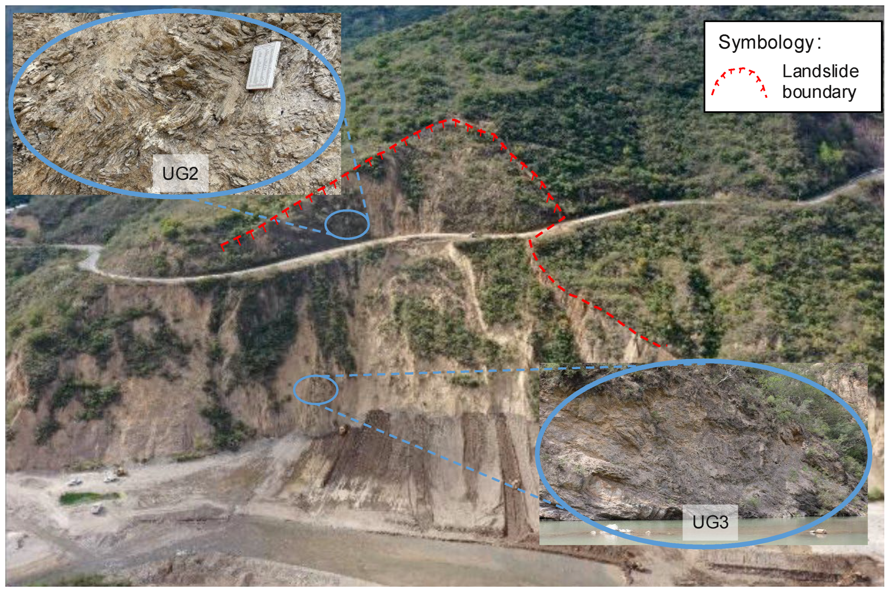
A landslide triggered by heavy rainfall blocked approximately 100 m of the Tuxtepec–Oaxaca highway (Federal Highway 175, ca. 17.31° N, 96.53° W), which crosses the Sierra Juárez, part of the Sierra Norte de Oaxaca mountain system, in the state of Oaxaca, southern Mexico, where landslides have repeatedly caused road closures. The failed area is located within a formation composed of a sequence of shales, calcareous sandstones, argillaceous limestones with a “flyschoide” appearance, and laminar marls (Figure 1). The proportion of shales to sandstones varies depending on the particular zone. The sandstones are coarse- to medium-grained, poorly sorted, and cemented by a calcareous matrix. The shales are laminated, thin-bedded, and highly fractured. Clayey limestones are gray in color and have a compact, folded structure. Figure 1 shows an image of the main geological formation and the occurred landslide.

The study area is characterized by steep mountainous terrain and the presence of the Río Grande at the toe of the slope. Hydrogeological behavior is primarily controlled by secondary permeability associated with fractures, bedding planes, and weathered zones within the shale and sandstone formations. During prolonged rainfall events, water infiltration through these preferential flow paths may promote groundwater recharge and pore pressure build-up within the rock mass. The resulting increase in pore-water pressures contributes to a reduction in effective stress and shear strength, thereby increasing the susceptibility of the slope to instability. These hydrogeological conditions were considered in the evaluation of the tunnel–slope system performance under rainfall-induced loading conditions.

A road tunnel was proposed as a mitigation measure to bypass the landslide-affected section and reduce the exposure of highway users to hazards associated with ground collapse. The tunnel alignment was located at four tunnel diameters from the slope to minimize interaction between the excavation and the unstable rock mass. The proposed tunnel is excavated through the fractured shale–sandstone–limestone sequence described above. Construction is planned to proceed according to the Conventional Tunneling Method [17], with a maximum advance of 2 m per cycle, using steel frames, shotcrete, and umbrella pipes as tunnel support. Given the highly fractured and heterogeneous character of the rock mass, the shallow cover relative to the tunnel span, and the proximity of the excavation to an unstable slope, the assumption of a fixed clearance of four tunnel diameters must be verified rather than taken as inherently sufficient. This motivates a detailed 3D numerical evaluation of the tunnel–slope interaction under both static and dynamic (seismic) conditions.

2. Methodology

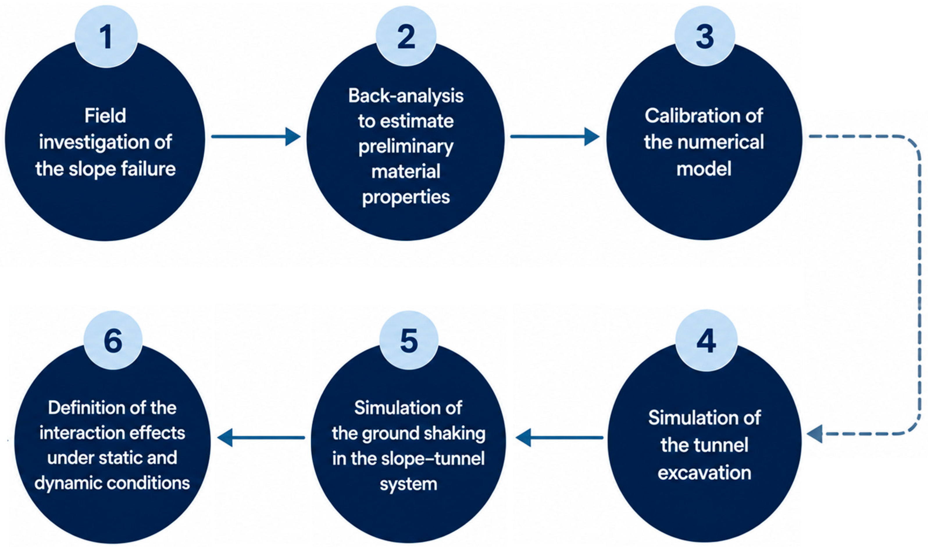
A performance-based assessment of the tunnel–slope system was carried out following the methodology illustrated in Figure 2. The procedure begins with a comprehensive field investigation of slope failure, including geological and geotechnical characterization of the fault zone to identify the mechanisms governing the observed instability. Based on these observations, a back-analysis was performed to estimate preliminary geomechanical properties capable of reproducing the observed failure conditions.

The preliminary parameters were subsequently compared with those obtained from laboratory testing and empirical correlations based on the Hoek–Brown failure criterion. These datasets were used to calibrate the numerical model until a satisfactory agreement was achieved between the simulated response and the observed field behavior, providing a representative set of material properties for subsequent analyses.

Once the numerical model was calibrated, the tunnel excavation process was simulated using a detailed three-dimensional numerical model that explicitly represents the geological units, the fault zone, the tunnel support system, and the excavation sequence. This stage was aimed at evaluating the influence of tunnel construction on the stability of the slope under static conditions.

Subsequently, the seismic response of the tunnel–slope system was evaluated by applying the critical ground-motion scenario defined for the study area based on the regional seismic hazard. The dynamic analyses allowed the coupled response of the slope and the underground structure to be investigated under earthquake loading.

Finally, the interaction effects between the tunnel and the unstable slope were evaluated under both static and seismic conditions. The system performance was assessed in terms of slope displacements, stability conditions, and the structural response of the tunnel lining, providing the basis for the performance-based evaluation presented in this study. For the tunnel structure, the diametral strain ratio (ΔD/D) was used to evaluate cross-sectional distortion, and in the longitudinal direction axial force demand in comparison with the structural capacity of the lining was used as performance index.

3. Rock Mass Characterization

The rock mass was classified using the Geological Strength Index (GSI), developed by Hoek and Brown [18], based on field observations. It exhibited characteristics of a flysch-type formation, consisting of alternating medium to thick limestone layers and thin shale strata. From the GSI parameter, and other rock strength parameters, it is possible to estimate the failure envelope according to the generalized Hoek–Brown model, which is defined by the following equation:

$${\sigma }_{cm}={{\sigma }^{\prime }}_3+{\sigma }_{ci}(m_b{\displaystyle \frac{{{\sigma }^{\prime }}_3}{{\sigma }_{ci}}}+s{)}^a$$

(1)

where σ_cm is the equivalent uniaxial compressive strength of the rock mass; σ_ci is the uniaxial compressive strength of the intact rock; and σ′₃ is the minor principal stress. Likewise, the values of $a,m_b$ and s are determined with the following equations:

$$a={\displaystyle \frac{1}{2}}+{\displaystyle \frac{1}{6}}(e^{{\displaystyle \frac{GSI}{15}}}-e^{-{\displaystyle \frac{20}{3}}})$$

(2)

$$m_b=m_i{e}^{{\displaystyle \frac{GSI-100}{28-14D}}}$$

(3)

$$s=e^{{\displaystyle \frac{GSI-100}{9-3D}}}$$

(4)

where GSI is the parameter that considers the structural characteristics of fracturing, the alteration state of the discontinuities, and the surface of the rock mass. In this case, a value of D = 0 is suggested when the excavation is carried out by mechanical or manual means for low-quality rocks, resulting in minimal impact on the surrounding rocks.

To define the uniaxial compressive strength of the intact rock, σ_ci, the values from laboratory tests performed on rock cores extracted from the boreholes were used.

For calculations using numerical methods, a Mohr–Coulomb failure criterion was established to represent the behavior of the rock mass. Therefore, the cohesion (c), internal friction angle ($\phi$), and Young’s modulus ($E_m$) parameters of the rock mass were estimated. The strength envelope of the rock mass was established according to the Generalized Hoek & Brown constitutive model, and, subsequently, the equivalent Mohr–Coulomb constitutive law was determined. The expressions used were as follows:

$$c={\displaystyle \frac{{\sigma }_{cm}[\left(1+2a\right)s+\left(1-a\right)m_b{{\sigma }^{\prime }}_{3n}](s+m_b{{\sigma }^{\prime }}_{3n}{)}^{a-1}}{\left(1+a\right)\left(2+a\right)\sqrt{1+\frac{6a{m}_b(s+m_b{{\sigma }^{\prime }}_{3n}{)}^{a-1}}{(1+a)(2+a)}}}}$$

(5)

$$\phi ={sin}^{-1}\left[{\displaystyle \frac{6a{m}_b(s+m_b{{\sigma }^{\prime }}_{3n}{)}^{a-1}}{2\left(1+a\right)\left(2+a\right)+6a{m}_b(s+m_b{{\sigma }^{\prime }}_{3n}{)}^{a-1}}}\right]$$

(6)

$$E_m\left(GPa\right)=\left(1-{\displaystyle \frac{D}{2}}\right)\sqrt{{\displaystyle \frac{{\sigma }_{ci}}{100}}}\ast {10}^{[{\displaystyle \frac{GSI-10}{40}}]}$$

(7)

where ${{\sigma }^{\prime }}_{3n}$ is determined with the following equation:

$${{\sigma }^{\prime }}_{3n}={\displaystyle \frac{{{\sigma }^{\prime }}_{3max}}{{\sigma }_{cm}}}$$

(8)

${{\sigma }^{\prime }}_{3max}$ is the maximum value of the confinement stress that can occur at the site.

Table 1. Summary of parameters of the generalized Hoek & Brown constitutive model for geotechnical units.

Geotechnical Units	Unit	σci (MPa)	GSI	mi	D
Slope deposits	UG1	NA	NA	NA	NA
Highly weathered shales and limestones	UG2	38.5	15	7	0
Moderately weathered shales and limestones	UG3	65.6	25	7	0

shows the estimated Hoek–Brown parameters.

In the table, σ_ci is the uniaxial compressive strength of the intact rock, GSI and D were described above, $m_i$ is a constant that depends on the type of rock, and UG is the geotechnical units.

Based on this data, Mohr–Coulomb equivalent parameters were stated (cohesion and friction angle), and Young’s modulus was calculated as a function of the Geological Strength Index (GSI).

Table 2. Initial geotechnical parameters used for analysis.

Layer	${\mathit{\gamma }}_{\mathit{n}}$ (kN/m3)	${\mathit{E}}_{\mathit{m}}$ [MPa]	ν	c [kPa]	φ [°]
Slope deposits (UG1)	20.0	100	0.35	30	35
Highly weathered shales and limestones (UG2)	24.0	770	0.30	300	34
Moderately weathered shales and limestones (UG3)	24.0	1850	0.30	300	40

shows the initial parameters used in the analyses. Stratigraphy for analysis was developed from field surveys, in situ tests, geophysical data, boreholes, and laboratory analyses to define layering and geomechanical properties. Three geotechnical units were identified (Table 2). Unit 1: Slope deposits; unit 2: highly weathered shales and limestones; and unit 3: moderately weathered shales and limestones.

In the table, γ_n is the unit weight of the material, Em is the Young’s modulus of the rock mass, ν the Poisson’s ratio, C is the cohesion, and φ the friction angle.

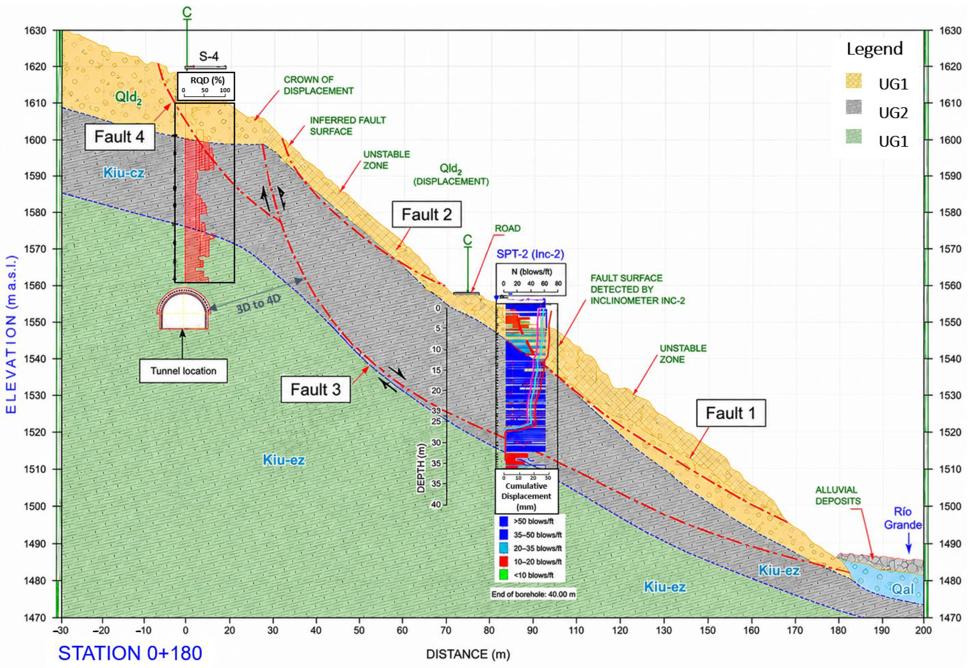
Figure 3 shows the geological–geotechnical profile of the landslide, the stratigraphy, the identified failure surfaces, and possible location of the tunnel.

4. Tunnel Project Features

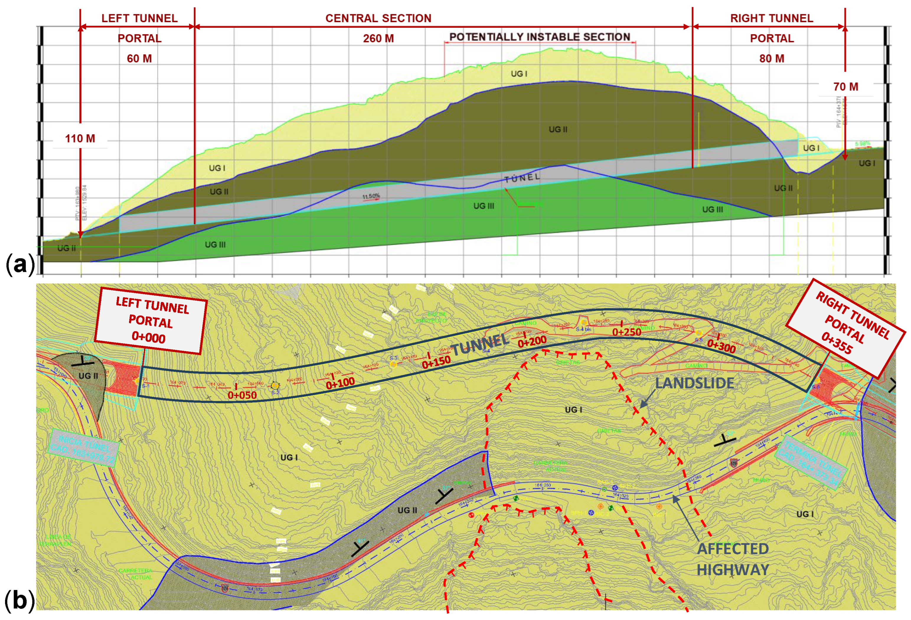
The proposed tunnel has a total length of 393.6 m, a width of 15.8 m, and a height of 9.5 m, with 355 m to be excavated according to the Conventional Tunneling Method [17]. Figure 4 depicts the location of the tunnel project regarding the landslide, the topography, the affected highway, and the stratigraphy.

During the tunneling process, maximum advance was defined based on the rock properties, and the used tunnel support elements consisted of steel frames, fiber-reinforced shotcrete, and umbrella pipes. The steel frames correspond to IR sections of steel grade A-572-50, with a yield strength fy = 350 MPa. The umbrella pipes (fore poling) consisted of N-80 steel pipes, 4 in. (ø) in diameter and 7 mm in wall thickness, grouted with a cement mortar of f′c = 20 MPa. The shotcrete had a design strength of f′c = 30 MPa, which is reinforced with steel fibers with a dosage of 30 kN/m³, to provide an energy absorption capacity of at least 1000 J. 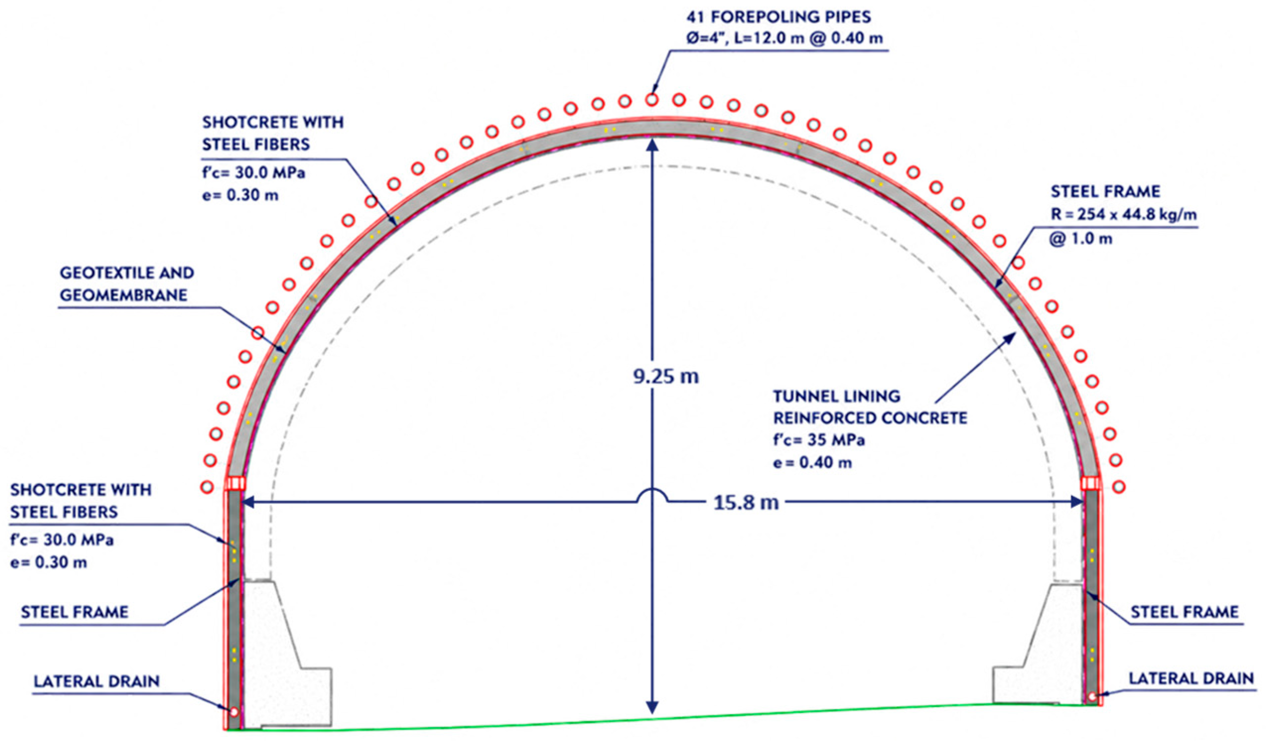Figure 5 depicts the cross section of the tunnel.

The tunnel excavation and support sequence considered three construction procedures (ST1, ST2, and ST3), all based on a top-heading and bench excavation stages, supported with shotcrete, steel frames and completed with waterproofing membranes and a final concrete lining once benching of the side cores is finished. In procedure ST1, the upper half-section is excavated by sides in 3 m increments with an initial layer of fiber-reinforced shotcrete, after which the opposite side of the upper half-section is completed in 1.5 m increments using shotcrete and steel frames; the left and then the right core are subsequently excavated with offset control, repeating the same support scheme before the final lining is placed. Procedure ST2 follows the same four-stage logic, but every 9 m, 41 umbrella pipes are installed as indicated in Figure 5, after which the entire upper half-section is excavated in 2 m increments; the central core is then excavated in increments of up to 4 m once the upper half-section is complete, and the left and right cores are subsequently benched in 3 m increments, with support and finishing works as described for ST1. Procedure ST3 excavates the upper half-section by sides, as in ST1, but in 2 m increments, followed by a central-pillar stage of the upper half-section at 1 m increments with shotcrete and steel frames; the central core is then benched once the upper half-section is complete, and the left and right cores are benched together in the final stage, with the same support and finishing works described above. After the tunneling is finished, the tunnel lining of reinforced concrete (f′c = 35 MPa) is installed.

5. Numerical Modeling

The simulations were developed in 2D and 3D numerical models in the software FLAC3D v. 6.0. The analyses were divided in three main stages, (1) back-analysis of the occurred landslide in the slope and validation of the geotechnical parameters, (2) simulation of the tunneling excavation process and verification of the impact in the slope stability, and (3) seismic simulation of the slope–tunnel system considering the most critical seismic scenario for the studied site according to the seismic hazard of the zone. Finally, the interaction effects in the slope–tunnel system are defined under static and dynamic conditions, in terms of displacements, safety factors, and tunnel lining forces.

Section 5.1 presents the main features of the back-analysis of the observed landslide, performed to calibrate the geomechanical properties of the rock mass and reproduce the failure conditions recorded in the field. Section 5.2 then presents the main features of the three-dimensional simulation of the tunnel excavation process, carried out to evaluate the influence of tunnel construction on slope stability under static conditions. Finally, Section 5.3 describes the details of the seismic slope–tunnel interaction analysis.

5.1. Back-Analysis of the Landslide

The SLIDE program, a specialized 2D limit equilibrium software for slope stability, was used initially to establish the failure surface and factor of safety, with the limit equilibrium method (LEM). This program enables the evaluation of the factor of safety (FS), of circular or non-circular slip surfaces on soil and rock slopes, analyzed through discretization with the slice method. Using multiple search and optimization algorithms, the analysis generates the minimum FS, which corresponds to the critical failure surface. Sensitivity analyses can also be performed, in which resistance parameters are varied to determine their impact on the FS.

The inverse analysis, based on the limit equilibrium method, was performed using sensitivity analysis, with the aim of finding the combinations of strength properties that resulted in a factor of safety (FS) ≈ 1. To carry out these analyses, a fixed friction angle was established, and the cohesion was varied within a specific range to obtain the cohesion vs. FS relationship. This analysis was repeated considering various friction angle values to obtain the cohesion and friction angle combinations that resulted in an FS ≈ 1. Dry and saturated conditions were considered in the slope body.

Once the possible combinations of strength parameters that could lead to slope failure were established, the analysis was performed with the FLAC3D model using the estimated strength and stiffness parameters, and the strength reduction method. Stability analyses were performed to reproduce the observed failure surfaces of Figure 3, varying the cohesion, and maintaining friction angle constant, until achieving a safety factor FS ≈ 1, considering both dry and saturated conditions. 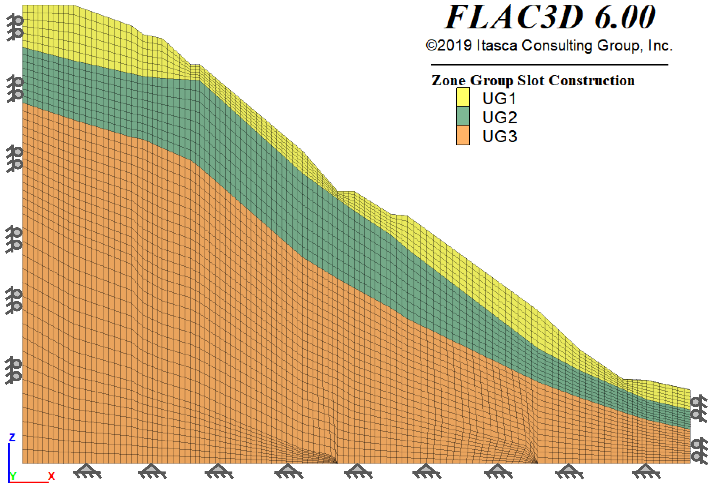Figure 6 shows the finite difference mesh used for the 2D slope assessed in FLAC3D, as well as the considered boundary conditions. Normal displacements were restricted along the lateral boundaries, while all translational degrees of freedom were fixed at the base of the model. The numerical domain used for the slope stability back-analysis extended approximately 255.58 m along the analyzed section. This dimension was selected to ensure that the observed failure mechanism developed away from the model boundaries and that boundary effects did not influence the predicted stability conditions.

Figure 7 presents the stability results of both methods (LEM and FLAC3D) with the cohesion–friction angle combination that reproduced the failure surface considering dry conditions. The failures developed were within the slope deposits at the toe and crest, with a failure cohesion of approximately 21 kPa, and a friction angle of 30°. The predicted mechanisms agreed with field observations, where initial sliding occurred at the lower slope, followed by instability at the upper slope prior to global collapse. It can also be highlighted that both methods adequately reproduced the inferred slip surface.

The next step was to evaluate the stability of the slope, assuming saturated conditions due to the rainy season. Hydrogeological behavior is primarily controlled by secondary permeability associated with fractures, bedding planes, and weathered zones within the shale and sandstone formations, and during prolonged rainfall events infiltration through these preferential flow paths promotes rapid groundwater recharge and a rise in the water table. Due to these conditions, the groundwater regime was idealized in the numerical analyses by means of a static phreatic surface corresponding to the fully saturated state of the slope. This represents a conservative upper bound condition, since it maximizes pore-water pressures and minimizes the effective stresses and shear strength available along the potential failure surface, with pore-water pressures assigned following a hydrostatic distribution below the assumed water table. This approach avoids the additional uncertainties associated with transient unsaturated-flow parameters while ensuring that the slope stability is evaluated under the most unfavorable groundwater condition. 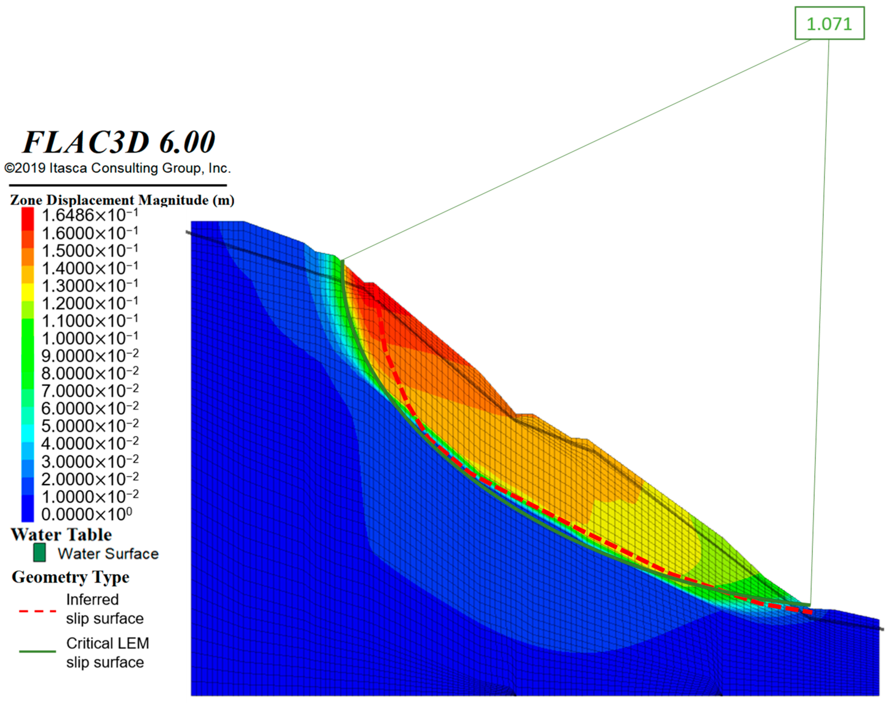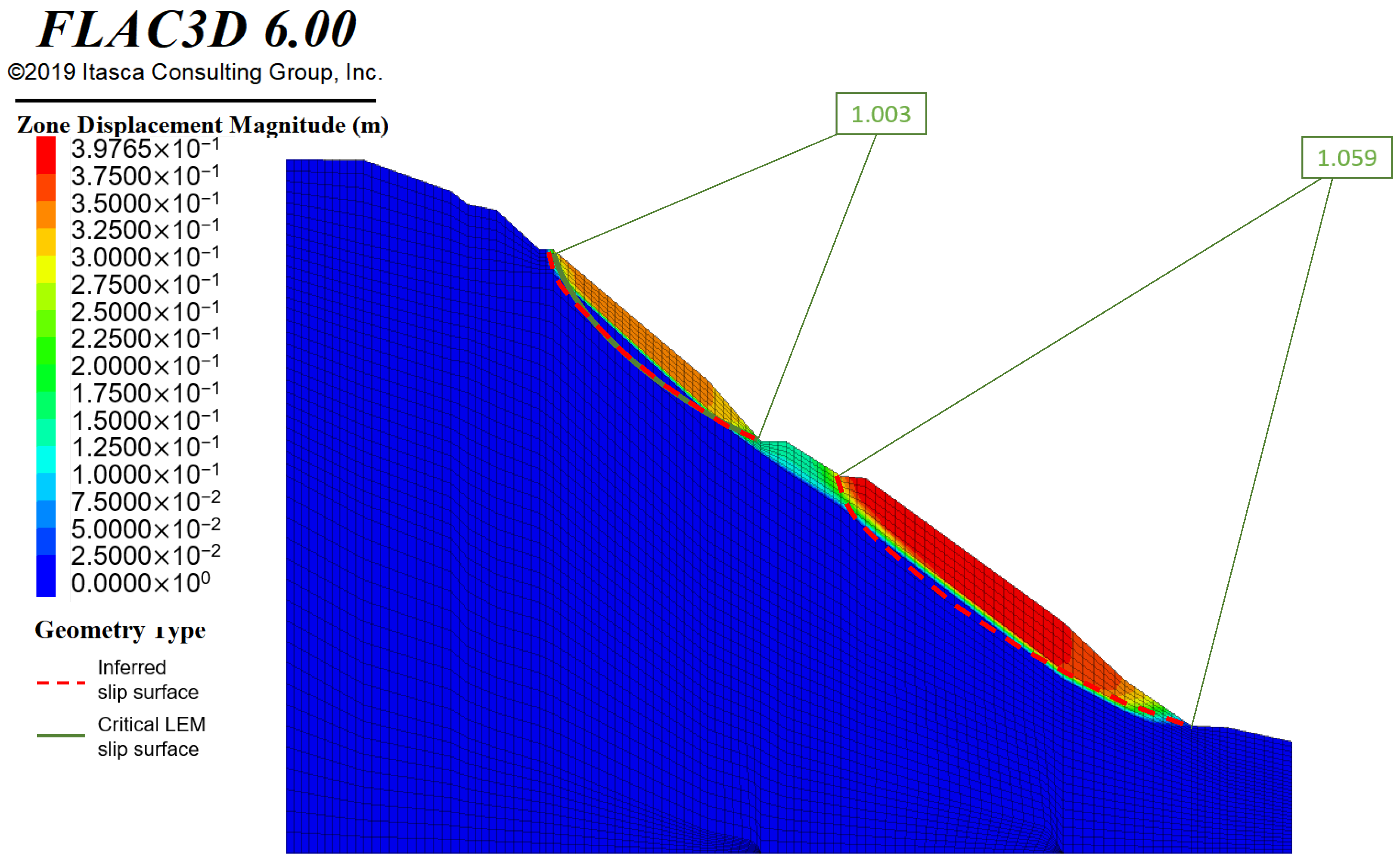Figure 8 presents the displacement contours from the FLAC model, and the critical slip surface from the LEM with the corresponding FS, where it can be appreciated that the failure mechanism calculated with both methods adequately reproduces the estimated failure with field observations. The results indicated a failure cohesion of approximately 154 kPa, and a friction angle of 34° for Geotechnical Unit 2.

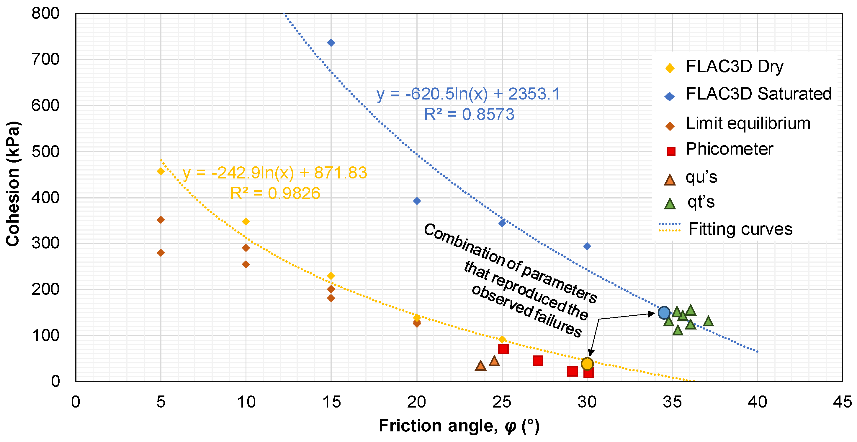
Figure 9 illustrates the summary graph that was generated after performing several analyses with FLAC3D and LEM, showing all possible combinations of parameters that could have caused the slope failure, both under dry and saturated conditions. The comparison between field data and back-analysis results showed that the global failure occurred during the rainy season, which corresponds to saturated conditions with FS ≈ 1, consistent with a critical stability state. In contrast, dry conditions adequately reproduced the shallow failures, which occurred progressively under dry conditions. Phicometer tests were carried out in the UG1, and laboratory unconfined compression, qu, and indirect tension, qt, (Brazilian) tests in UG2, to verify the values of the proposed parameters, and good fit was found, as depicted in Figure 9.

Overall, the multi-source calibration approach, which integrate geological mapping, borehole data, laboratory testing, geophysical surveys, phicometer measurements, limit-equilibrium analyses, and three-dimensional finite difference back-analysis, provides a robust basis for validating the geomechanical parameters used in this study. The calibrated model reproduced both the observed failure surface geometry and the progressive instability pattern documented in the field, yielding factors of safety close to unity under saturated conditions, consistent with the landslide’s occurrence during the rainy season, and only localized shallow failures under dry conditions, in agreement with field evidence. Although direct monitoring data for the proposed tunnel are not yet available, since construction has not started, the consistency between the back-analysis results and the documented failure conditions confirms that the adopted strength and stiffness parameters are representative of the in situ rock mass behavior, supporting their use in the subsequent numerical simulations of the tunnel–slope system under static and seismic loading conditions. The final calibrated geotechnical parameters are included in

Table 3. Calibrated geotechnical parameters used for numerical analyses.

Unit	γ (kN/m3)	Em [MPa]	ν	Cohesion [kPa]	φ [°]
Slope deposits	20.0	100	0.35	21	30
Highly weathered shales and limestones (unaltered)	24.0	800	0.30	154	34
Highly weathered shales and limestones (residual)	24.0	790	0.30	46	30
Moderately weathered shales and limestones	24.0	1410	0.30	167	40

.

5.2. Tunneling Process Simulation

For the tunneling simulation, a three-dimensional numerical model was developed to assess ground stability in the slope body, and around the tunnel excavation, and also for the performance of the support system during tunnel excavation. Owing to the tunnel length, the model was divided into three sections according to Figure 4a: left tunnel portal, central section, and right tunnel portal. According to the aims and scope of the study, which consists in characterizing the slope–tunnel interaction under static and dynamic conditions, only the results of the central section are included in this paper, since the tunnel portals imply a different and complex type of interaction. The portal areas are influenced by shallower overburden and proximity to the slope face and are also far away from the landslide-affected zone where the central section is located. Consequently, the analyses were focused on the central section.

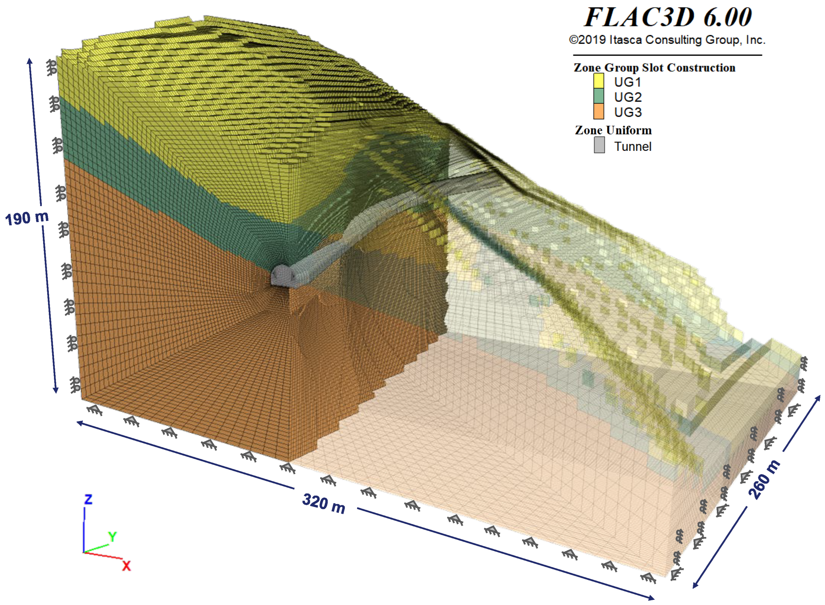
Figure 10 illustrates the finite difference mesh used for the simulation of the tunneling process. The dimensions of the numerical domain were selected to ensure that the model boundaries were located sufficiently far from the tunnel excavation and the critical slope instability zone, thereby minimizing potential boundary effects on the computed response. In the transverse direction, the tunnel has an average distance of 120 m to the lateral boundaries of the model.

Boundary conditions were assigned following standard numerical modeling practices. Normal displacements were restricted along the lateral boundaries, while all translational degrees of freedom were fixed at the base of the model. Gravity loading was then applied to establish the initial in situ stress field prior to excavation and dynamic analyses. The adopted domain dimensions and boundary conditions allowed the predicted deformation patterns and failure mechanisms to develop entirely within the interior region of the model, indicating negligible influence of the model boundaries on the numerical results.

The rock mass was simulated using the Mohr–Coulomb constitutive model, which has been widely applied in geotechnical engineering due to its simplicity and its ability to represent the overall strength and deformation characteristics of geomaterials using a limited set of engineering parameters. Nevertheless, the model presents certain limitations when applied to highly fractured rock masses. In particular, it does not explicitly account for strain-softening behavior, progressive damage accumulation, anisotropic mechanical response, or the presence and propagation of individual discontinuities. Consequently, local failure mechanisms associated with joint-controlled behavior may not be fully captured.

Although the geological investigation identified four principal discontinuity sets and stereographic analyses indicated that some orientations could potentially generate wedge-type instabilities, detailed field observations showed that the rock mass is extremely fractured, highly weathered, and heterogeneous, with discontinuities of limited persistence and extensive fragmentation; consequently, no continuous structural surfaces capable of controlling large-scale kinematic failure were identified. Given that the scale of the investigated slope failure and tunnel excavation is substantially larger than the characteristic block size defined by the discontinuity network, the rock mass was represented as an equivalent continuum, in which the mechanical response is governed primarily by the integral behavior of the fractured mass rather than by the movement of individual blocks. Then, the influence of discontinuities was incorporated indirectly through the geomechanical characterization, combining geological mapping, GSI classification, laboratory testing, and back-analysis of the observed landslide to derive reduced strength and deformability parameters; the adopted Mohr–Coulomb properties therefore represent the equivalent mechanical behavior of the fractured and weathered rock mass, including the degradation associated with discontinuity density, weathering, and structural disturbance.

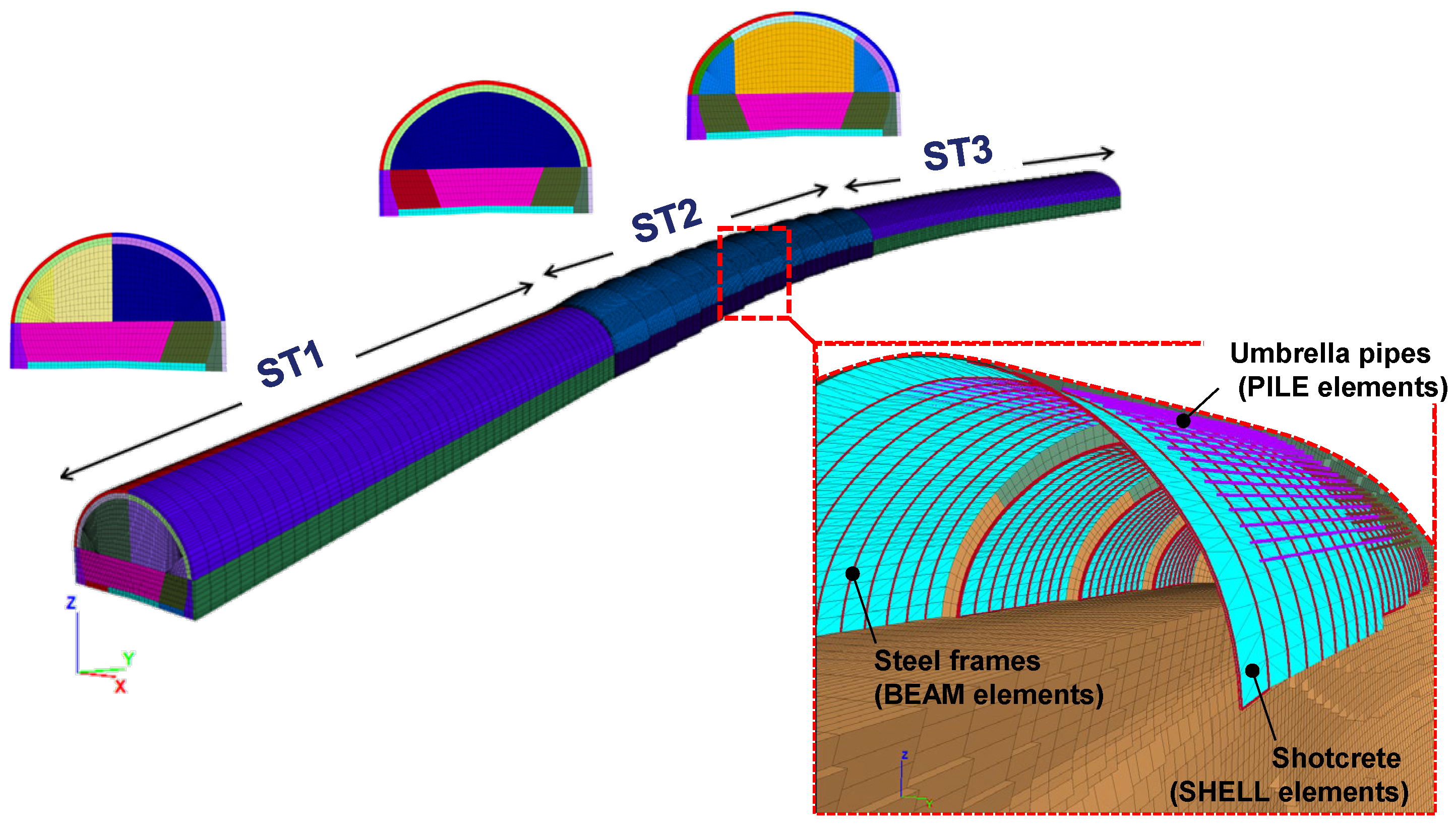
Figure 11 shows the construction stages along the tunnel considered in the numerical model according to Section 4, as well as the support elements. There, the definition of the cross-section excavation stages according to procedures ST1, ST2, and ST3 can be appreciated, where each color represents a different excavation stage. At each stage of the numerical analysis, calculations were continued until a stable equilibrium condition was achieved. Convergence was verified by monitoring the stabilization of displacements and stresses throughout the model prior to the execution of subsequent excavation or dynamic loading stages. This procedure ensured that the computed response reflected the mechanical behavior of the tunnel–slope system rather than numerical artifacts associated with incomplete equilibrium conditions.

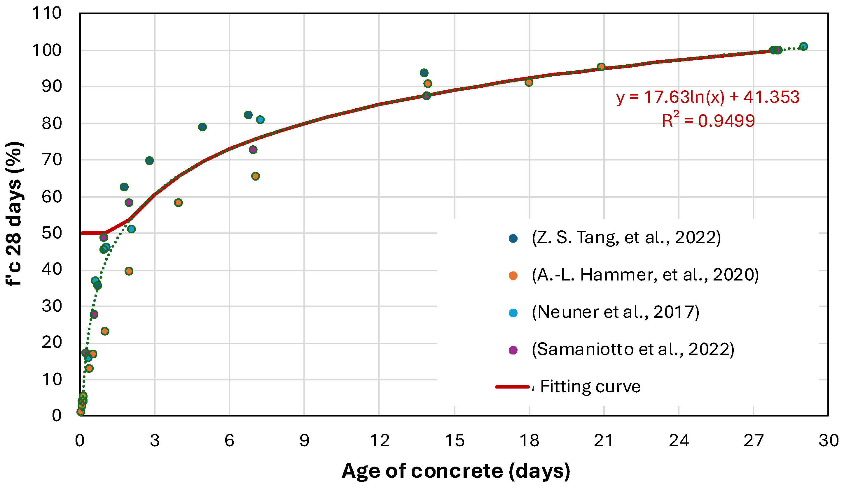
Regarding the simulation of the support elements, BEAM and PILE elements were used to represent steel frames and umbrella pipes, respectively, considering linear elastic behavior according to the material properties described in Section 4. To model the shotcrete, SHELL elements were used, and to adequately represent its behavior, the time-dependent strength gain was simulated, considering a daily excavation advance. Figure 12 shows the shotcrete strength development curve as a function of setting time that was adopted in the simulation. Figure 11 shows a view of the structural elements used in the numerical model.

5.3. Seismic Slope–Tunnel Interaction Simulation

Finally, the seismic evaluation was made for the tunnel–slope system, considering the output of the tunnel excavation process simulation under monotonic loading as the initial condition, to adequately represent the stress and strain initial states.

Site response analyses were conducted to verify the seismic demand on the tunnel support system, and the impact of the tunnel on the slope stability. Three geotechnical units were defined based on the geological model, with shear wave velocities, Vs, assigned from geophysical data (

Table 4. Dynamic properties of geotechnical units.

Unit	γ (ton/m3)	ν	Vs (m/s)
Slope deposits (UG1)	2.0	0.35	250–400
Highly weathered shales and limestones (UG2)	2.4	0.3	400–600
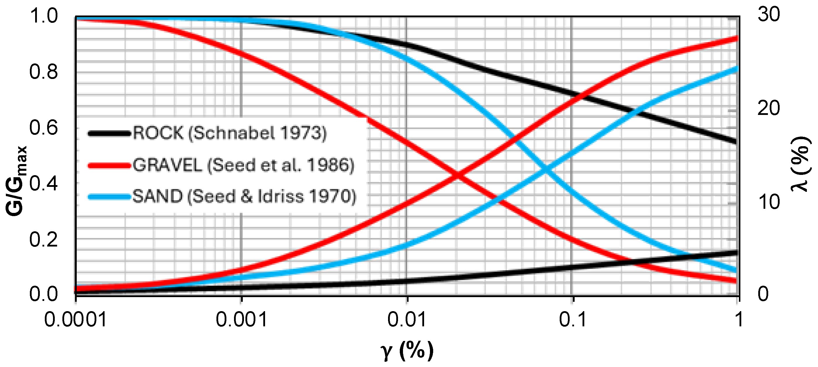
Moderately weathered shales and limestones (UG3)	2.4	0.3	600–800

). Due to the lack of dynamic laboratory tests, shear modulus degradation (G/Gmax) and damping ratio (λ) curves were adopted from the literature according to material type. Figure 13 shows the curves used. The rock curves were used for both units of shales and limestones (UG2 and UG3) and the gravel and sand curves for the slope deposits (UG1).

The seismic environment was defined using the deterministic approach, and ground motion prediction models [26,27], which were calibrated with records from a rock-site station near the studied site, verifying that the spectral forms were similar.

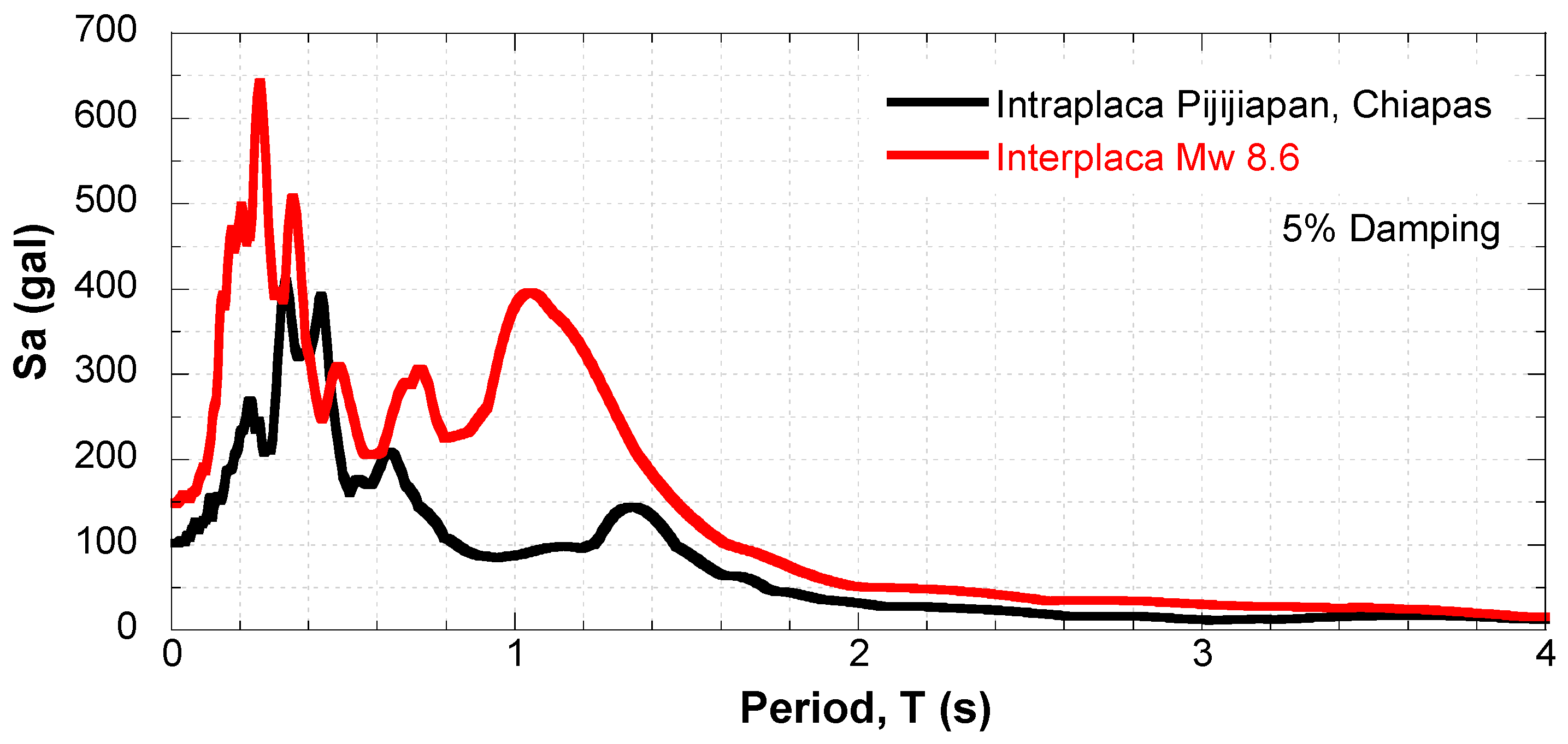
Two different types of seismic sources were considered in the analyses, intraplate and interface events. In the case of the intraplate earthquake, attenuation models showed reasonable agreement, but they underestimated pseudo-acceleration at some periods in comparison to the seismic record that generates the maximum accelerations in the reference station; therefore, the seismic record was used directly as input motion. This corresponds to the Mw = 8.2 Pijijiapan (Chiapas) intraplate earthquake. For the maximum interplate scenario (Mw 8.6), PGA was estimated using attenuation models [26,27], and the Crucecita (Oaxaca) record was scaled accordingly, as it represents the largest interplate PGA recorded near the potential rupture zone. The resulting response spectra are shown in Figure 14. Finally, the input motions applied at the base of the model were defined through deconvolution with the program SHAKE [28] and applied as a stress time history according to the compliant base approach [29,30]. Only the results corresponding to scaled interplate events are shown in this paper since they generate the greatest seismic motions.

Since the objective of the dynamic analyses was to evaluate the overall performance of the tunnel–slope system under a representative design earthquake scenario, rather than to perform a comprehensive seismic hazard sensitivity assessment, the seismic input corresponds to the most severe ground motion considered in the study, providing a conservative basis for evaluating tunnel stability and slope response under dynamic loading. It is acknowledged that variations in seismic intensity, frequency content, duration, and input direction may affect the magnitude and distribution of deformations. However, a systematic parametric evaluation of these variables was beyond the scope of the present study, which can be further analyzed in future research.

For the dynamic response of the tunnel–slope system simulated in FLAC3D, the nonlinear behavior of the geomaterials was approximated through the equivalent-linear method in the time domain, with ground motions applied in three orthogonal directions.

To ensure accurate transmission of seismic waves through the mesh, the maximum element size, Δl, was set following the criterion of Kuhlemeyer and Lysmer [31], which requires Δl to remain below one-fifth of the shortest wavelength of interest, λ = Vs/fmax, with fmax being the highest frequency carrying significant energy in the input motion. Since the acceleration time histories used in this study concentrate their energy between approximately 0.6 and 10 Hz, and the lowest average shear-wave velocity among the geomaterials was near 250 m/s, a maximum element size of 5.0 m was adopted.

Degradation of shear modulus with increasing strain during shaking was captured using FLAC3D’s built-in “Sig3” hysteretic formulation. This formulation is not a complete constitutive law on its own, but it can be used as a complement of plasticity models such as the Mohr–Coulomb, to supplement damping during the ground shaking although the stress paths remain in the elastic region. The underlying assumption treats the material as an ideal soil, in which stress depends only on the current deformation rather than on number of cycles. Under this assumption, the degradation curve can be expressed incrementally as τ_n/γ = G/Gmax, with τ_n denoting the normalized shear stress, γ the shear strain, and G/Gmax the normalized secant shear modulus. Equation (9) presents the Sig3 formulation adopted here.

$${\displaystyle \frac{G}{G_{max}}}={\displaystyle \frac{a}{1+e^{\left(-\frac{L-x_0}{b}\right)}}}$$

(9)

where L is the logarithmic strain, L = log10(γ), and the coefficients a, b, and x0 were calibrated iteratively so that the resulting degradation curve matched the target G/Gmax data. Because damping in this formulation follows directly from the shape of the hysteresis loop rather than fitted independently, the calibration prioritized the G/Gmax curves, obtained via a least-squares fit.

Radiation damping and the suppression of spurious wave reflections were handled by assigning quiet (viscous) boundaries at the base of the model, following the formulation of Lysmer and Kuhlemeyer [31], while the lateral boundaries used FLAC3D’s free-field condition. This approach couples a free-field grid that shares material properties of the model’s lateral edges to the main grid through viscous dashpots, transferring the free-field grid’s unbalanced forces onto the model boundary. As a result, upward-propagating plane waves pass through the boundary without distortion, since the free-field grid reproduces the response of a boundary embedded in an infinite medium.

6. Tunneling Simulation Results

6.1. Displacements

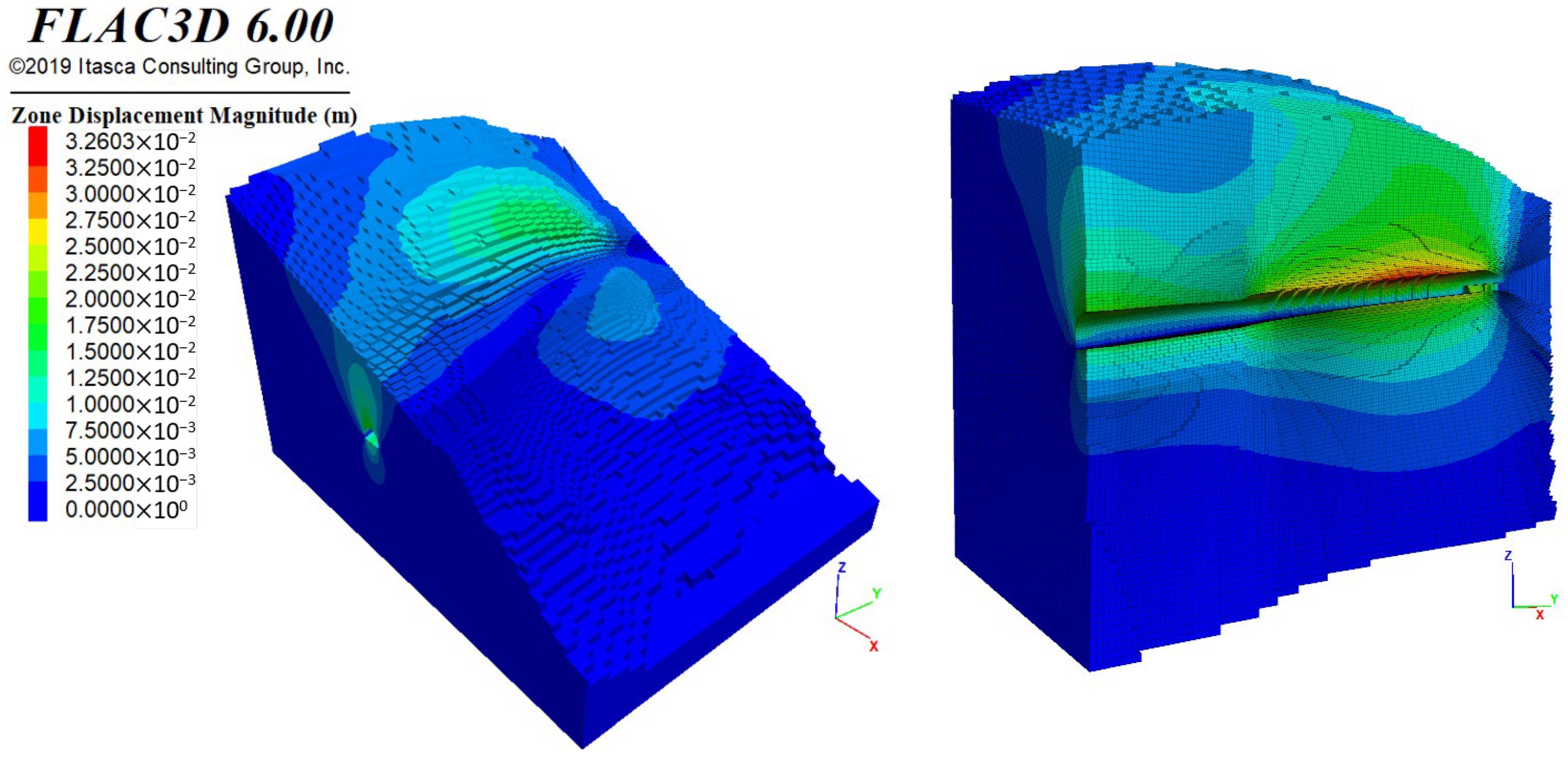
Ground displacements were first analyzed. At the end of excavation, maximum displacements of about 3.26 cm were calculated at the tunnel crown, particularly within the Geotechnical Unit 2, in the section where the tunnel is closer to the landslide. Regarding the slope displacement, the maximum calculated value is around 1.5 cm. These displacements result from stress release during excavation in a zone of lower stiffness. Figure 15 shows the distribution of the displacement obtained at the end of the tunneling simulation. The computed magnitudes, concentrated in the lower-stiffness Geotechnical Unit 2, are consistent with the deconfinement mechanism described by Causse et al. [12], whose parametric analyses showed that the stress release induced by tunnel excavation destabilizes the surrounding slope, with the degree of tunnel–slope interaction increasing markedly when the tunnel lies within approximately 1.5 diameters of the slope surface. Nevertheless, in this case, the tunnel is around 4 diameters away, for which there is some influence of the tunnel excavation on the slope behavior without generating instability.

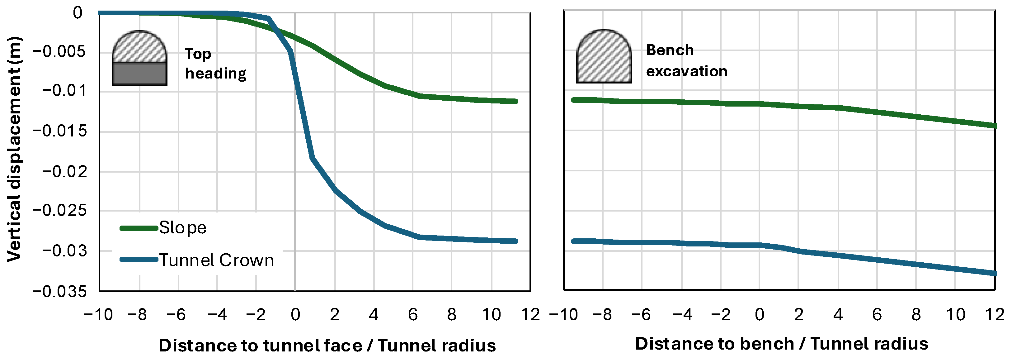
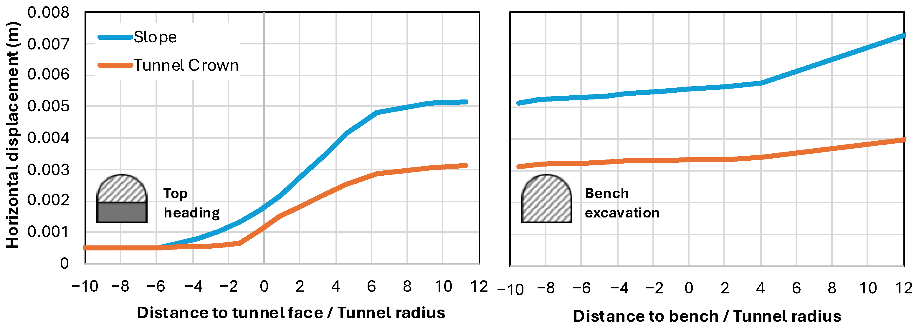
To analyze with more detail the evolution of the displacements in the slope and in the tunnel, in the identified critical section, longitudinal displacement profiles, LDPs, were calculated in both locations. Those show the evolution of displacements as the excavation gets closer to the analyzed section. Figure 16 shows the LDP for the vertical displacement and Figure 17 for the horizontal displacements. First, it can be noted that the vertical is such that governs the deformations in both the tunnel and the slope. Then it can be stated that the deformation in the slope is associated with the stress redistribution caused by the tunnel excavation, rather than the instability. This interpretation agrees with the field evidence gathered at the Val di Sambro twin tunnels [32], where tunneling temporarily accelerated pre-existing extremely slow landslide movements through stress redistribution, and displacement rates decreased progressively as the tunnel face moved away from the monitored sections.

Another feature that can be highlighted from Figure 16 and Figure 17 is that the displacements stabilize when the tunnel face is 6 radii from the analyzed section in both vertical and horizontal displacements. A similarly bounded zone of influence of the advancing face was observed through field monitoring at the Val di Sambro tunnels, where the maximum displacement rates were recorded for face–instrument distances ranging from −50 m to 100 m, decreasing significantly beyond 200 m and becoming negligible at distances larger than 400 m [32]. However, the direction of the horizontal displacements is downwards along the slope. It should be noted that, if the response of the tunnel–slope system was symmetric, the stress redistribution would essentially produce vertical displacements, with the horizontal components canceling each other out; hence, the systematic downslope orientation of the horizontal displacements evidences the asymmetric response induced by the sloping ground surface. This is in agreement with Causse et al. [12], who reported anisotropic convergence and deformation patterns around tunnels excavated within slopes, with maximum values toward the downhill side. Then, it can be possible that the slope could become unstable due to the tunnel excavation influence if the material would have lower strength values. This possibility is supported by the parametric analyses of Causse et al. [12], which show that slope destabilization intensifies with the amount of deconfinement allowed before lining installation, and that the maximum shear strains in the surrounding ground concentrate on the downhill side of the excavation, in agreement with the downslope orientation of the horizontal displacements computed here. To analyze that possibility, further parametric analyses considering reduced strength parameters or greater excavation lengths can be made in future research; nevertheless, that is beyond the scope of the current study.

6.2. Safety Factors

Safety factors were calculated at intermediate construction stages to evaluate tunnel face and slope stability at the identified critical section. The capacity-to-demand criterion proposed by Mayoral [33] was used to determine the factor of safety, and is expressed as follows:

$$FS={\displaystyle \frac{{\tau }_{cap}}{{\tau }_{act}}}$$

(10)

where

${\tau }_{cap}$	$=c+p^{\prime }\mathit{tan}\phi$
${\tau }_{act}$	$={\displaystyle \frac{1}{3}}\sqrt{{\left({\sigma }_1-{\sigma }_2\right)}^2+{\left({\sigma }_2-{\sigma }_3\right)}^2+{\left({\sigma }_1-{\sigma }_3\right)}^2}$
$p^{\prime }$	$=\left({\sigma }_1+{\sigma }_2+{\sigma }_3\right)/3$
${\sigma }_1,{\sigma }_2,{\sigma }_3$	= Principal stresses

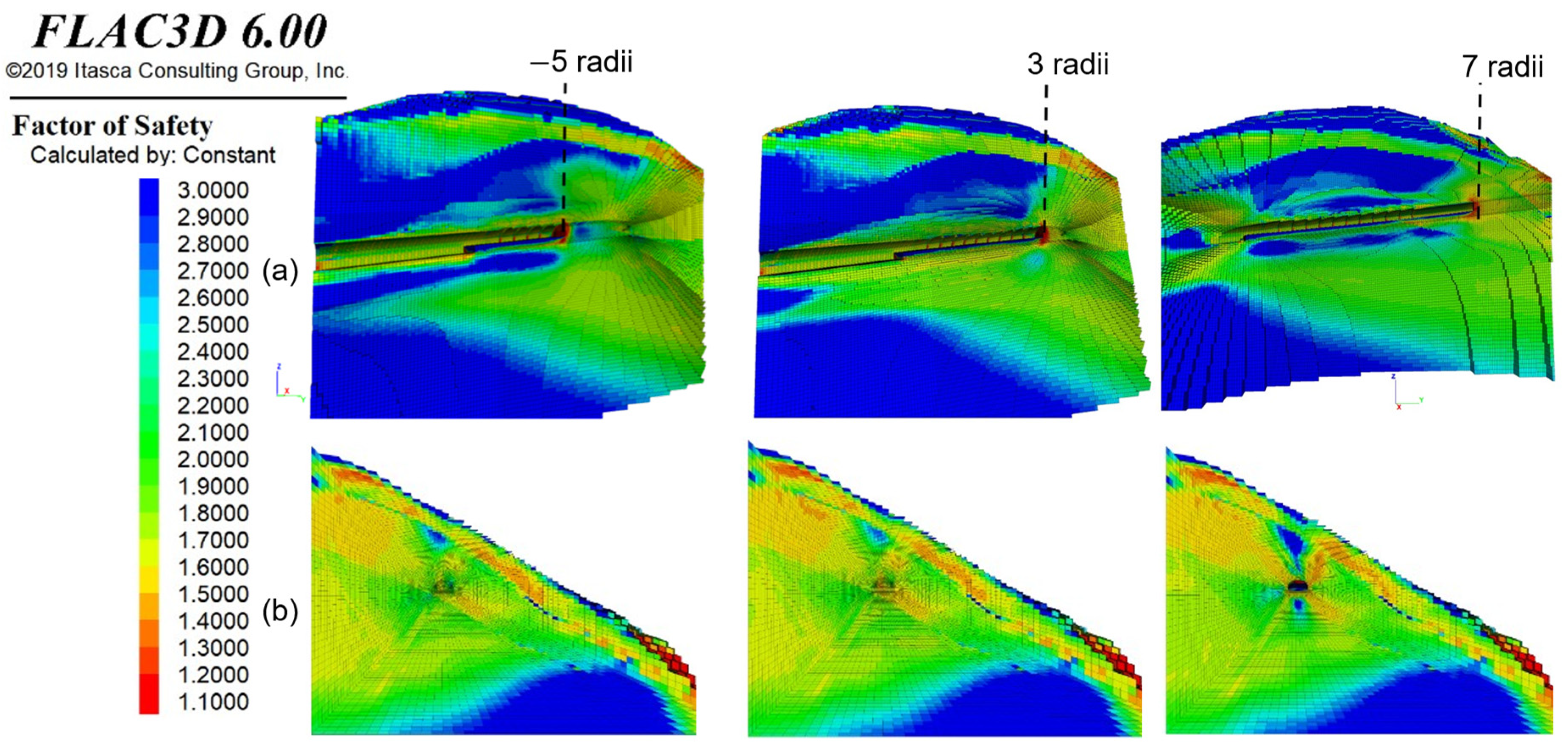
Figure 18a shows the results at three different intermediate steps, where the safety factors are critical at the tunnel face, and Figure 18b shows the results at the same steps but in a transversal view to visualize the variation in safety factors along the slope.

FS values around 1.6 indicate adequate global stability of the excavation. However, lower values close to 1.1 occur at the tunnel face during all construction stages, representing the most critical condition. Despite this, no global failure mechanism develops above the crown, suggesting that any instability would likely be limited to local spalling or minor detachments at the tunnel face. On the other hand, safety factors along the slope remain almost without changes as the tunnel excavation progresses, with values around 1.45. The last step when the tunnel face is 7 radii ahead of the analyzed section shows two critical zones at the right of the tunnel, that extend upward and downward, where safety factors are clearly lower than in the adjacent zones. The location of these zones agrees with the parametric results of Causse et al. [12], who found that the maximum shear deformations in the ground surrounding a tunnel excavated within a slope systematically concentrate on the downhill side of the excavation, near the spring line and the sidewall base. These zones are very close to the zones of lower safety factors of the slope, but, fortunately, they do not interact with each other. In the case that those zones could overlap, the slope stability could be seriously influenced, since the increment in acting shear stress, $∆{\tau }_{act}$, generated by the tunnel excavation, could reduce the safety factors of the slope, where they are already lower. In this regard, Causse et al. [12] showed that the shear slip surface developed around the tunnel grows as the deconfinement allowed before lining installation increases, so the potential coalescence of both low-safety-factor zones cannot be ruled out under less favorable construction procedures or strength conditions. To analyze that possibility, further parametric analyses considering reduced strength parameters or multiple positions of the tunnel regarding the slope can be made in future research; nevertheless, that is beyond the scope of the current study.

In conclusion, the tunneling process will not impact on the global stability of the slope, as can be seen in the displacements and safety factor contours. Therefore, the localization of low safety factors in a few portions at the tunnel face demonstrates that slope stability is not highly impacted by the tunnel excavation, since the changes in safety factors in the slope body during the excavation are almost negligible. This behavior contrasts with the case of the Val di Sambro twin tunnels [32], in which the tunnels were included in the moving mass and intersected the sliding surfaces of the landslide bodies; consequently, the excavation accelerated the movements along those surfaces, reaching rates of up to 40 mm/month at the ground surface and damaging the final lining. The geometric separation between the low-safety-factor zones around the tunnel and those within the slope, together with the stability reserve of the slope (FS ≈ 1.45), explains the negligible impact of tunneling computed in the present case.

It is worth mentioning that, in the case of the tunnel portals, tunnel face stability is the geotechnical feature that governs the tunneling process, since the amount of deconfinement around the excavation is greater and the possibility of a global failure increases. Nevertheless, those sections were not included since the tunnel portals imply different and complex interactions.

7. Seismic Slope–Tunnel Interaction Results

For underground structures with circular or semi-circular cross-sections, many standards use the diameter strain ratio as an evaluation index, defined as the ratio of convergence, ∆D, to the original diameter D:

$${\displaystyle \frac{∆D}{D}}={\displaystyle \frac{{\gamma }_{max}}{2}}$$

(11)

As defined in Equation (11), the diameter strain ratio can be calculated as a function of the maximum distortion of the tunnel ${\gamma }_{max}$, which can be obtained from unidimensional propagation analyses, when the tunnel stiffness is similar to that of the soil. Nevertheless, for more accurate approximation, the effects of soil–structure interaction should be considered. Typical tunnel-lining seismic design checks use deformation-based limits, and a commonly cited ovalization tolerance is about 1% [34]. A recent performance-based framework proposed diameter change-rate limits of 1/1850, 1/320, 1/180, 1/160, and 1/130 across five performance levels from basic intact to severely damaged [35]. Regarding the longitudinal behavior, the maximum axial force reached during the earthquake must not exceed the lining structural capacity [36].

Simulations of the tunnel’s seismic response were performed using three-dimensional finite difference models of the critical zones. These simulations were conducted after the completion of the final tunnel lining stages, as part of the construction process simulation, to accurately represent the stress and strain fields around the lining.

7.1. Slope Performance During the Earthquake

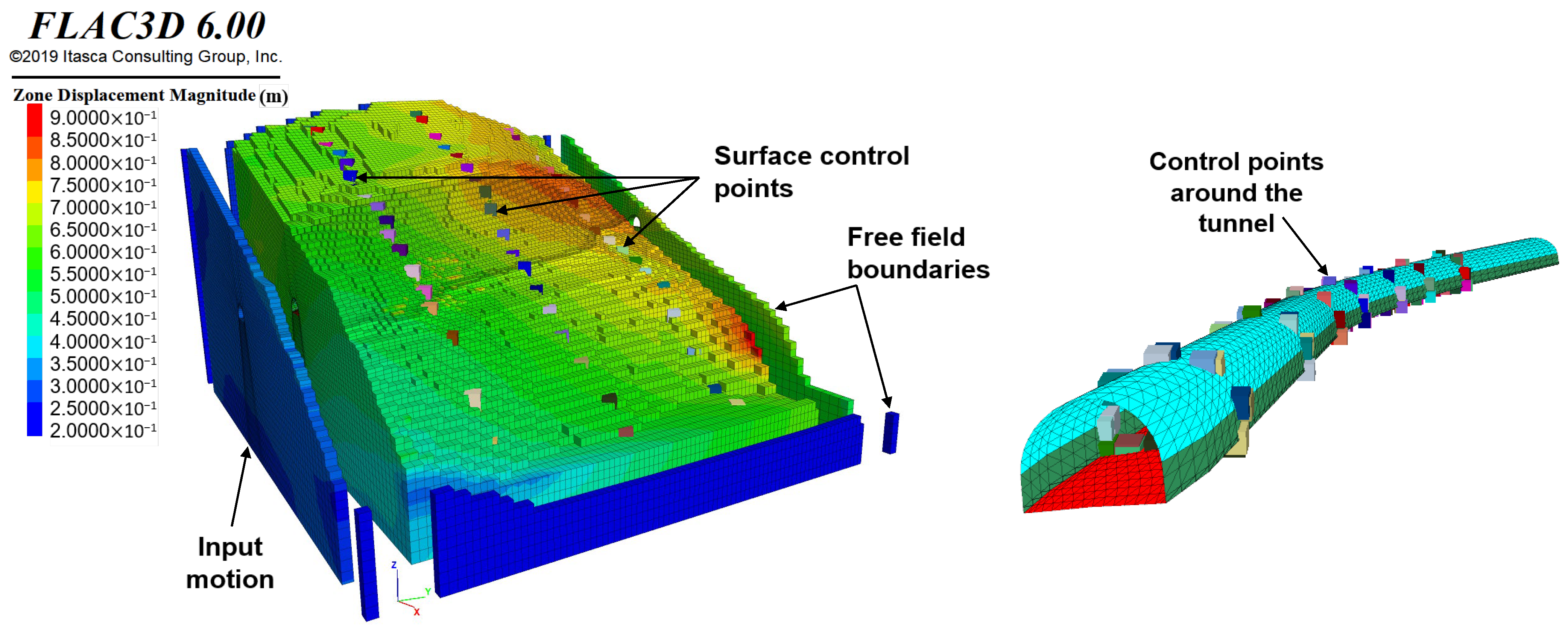
To monitor the behavior of the ground and the tunnel in terms of displacements during the earthquake simulation, control points were placed in three sections: the left portal, at the central section, and at the right portal. Figure 19 shows the location of these points in the model, as well as the boundary conditions considered for the analysis, according to the description of Section 5.3.

It should be noted that the use of stiffness degradation and damping curves from the published literature introduces uncertainty in the predicted accelerations, deformations, and lining force demands. Nevertheless, the small-strain stiffness of the geotechnical units was directly measured through geophysical surveys, so the adopted curves govern only the strain-dependent degradation relative to a measured baseline, and the seismic evaluation was performed for the most critical deterministic scenario derived from the regional seismic hazard, which partially envelopes the variability associated with the dynamic properties.

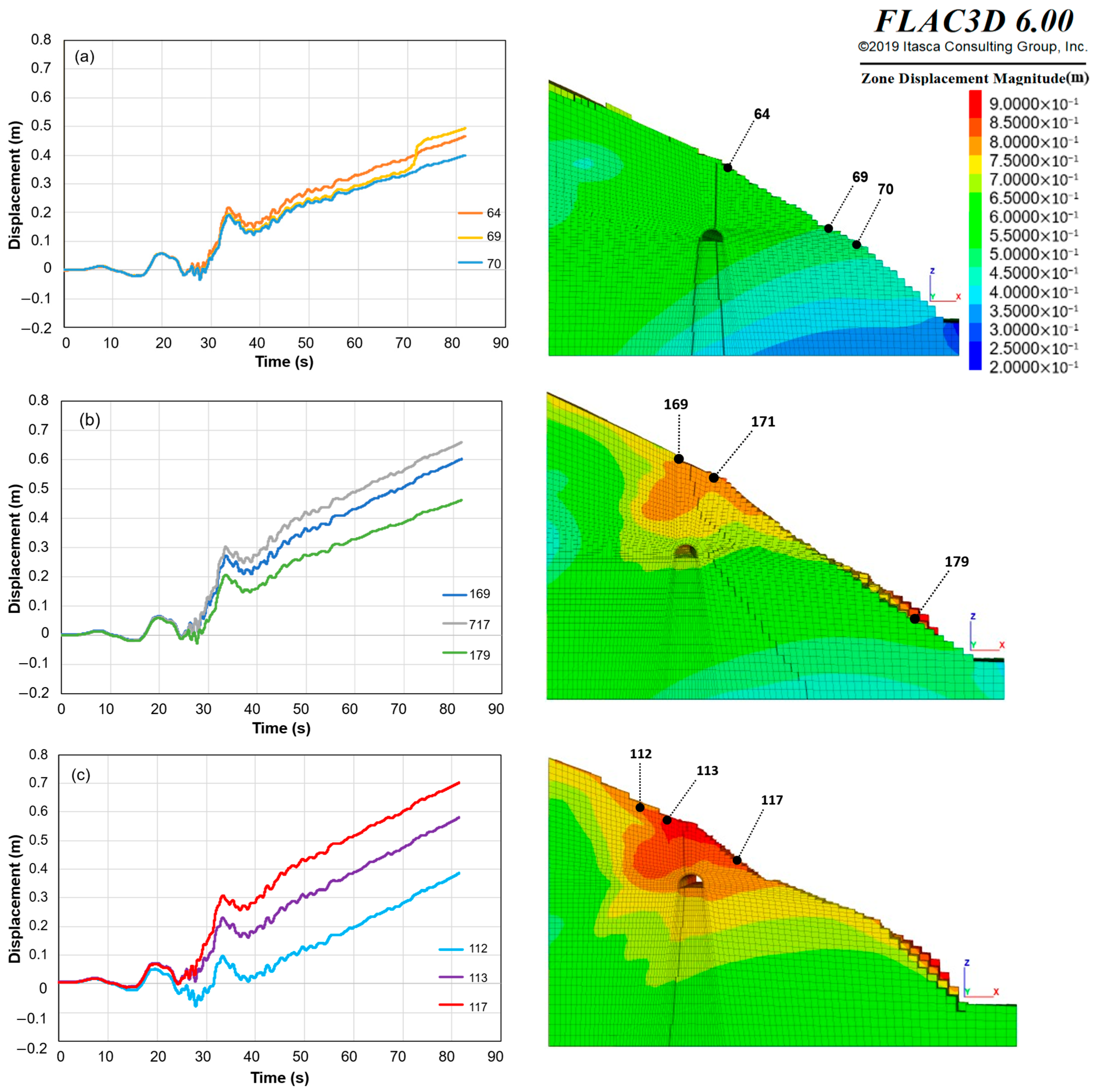
The displacement histories at the slope surface are depicted in Figure 20, showing that all monitored sections exhibit permanent displacements following the earthquake. This behavior indicates accumulation of plastic deformation within the slope mass [37]. From all the sections, the one located at the right tunnel portal presents the greatest accumulated displacements, reaching values up to 70 cm. This can be associated with the proximity of the tunnel to the failure surface, which affects slope stability due to shear stress concentrations during construction, and confining stress reductions. In addition, shaking table tests on bias tunnel–slope systems have shown that the peak ground acceleration amplification factor increases as the ground near the slope surface approaches the tunnel [38], which contributes to concentrating the seismic demand in the shallow zones near the portals. Given the pre-existing instability of the slope, the occurrence of large irreversible displacements of this magnitude under seismic loading suggests that the slope is susceptible to progressive failure following the earthquake. This interpretation is consistent with recent shaking table and numerical studies of tunnel–slope systems: Li et al. [39] observed that, under sustained seismic loading, deformation and damage gradually expand from localized areas to the entire slope in a progressive, cumulative failure evolution, with slope displacements roughly an order of magnitude greater than those of the tunnel. Similarly, Xin et al. [40] identified the failure mechanism of tunnel–slope systems as a sequence of cracking damage, damage accumulation, sliding deformation, and structural failure.

7.2. Lining Performance During the Earthquake

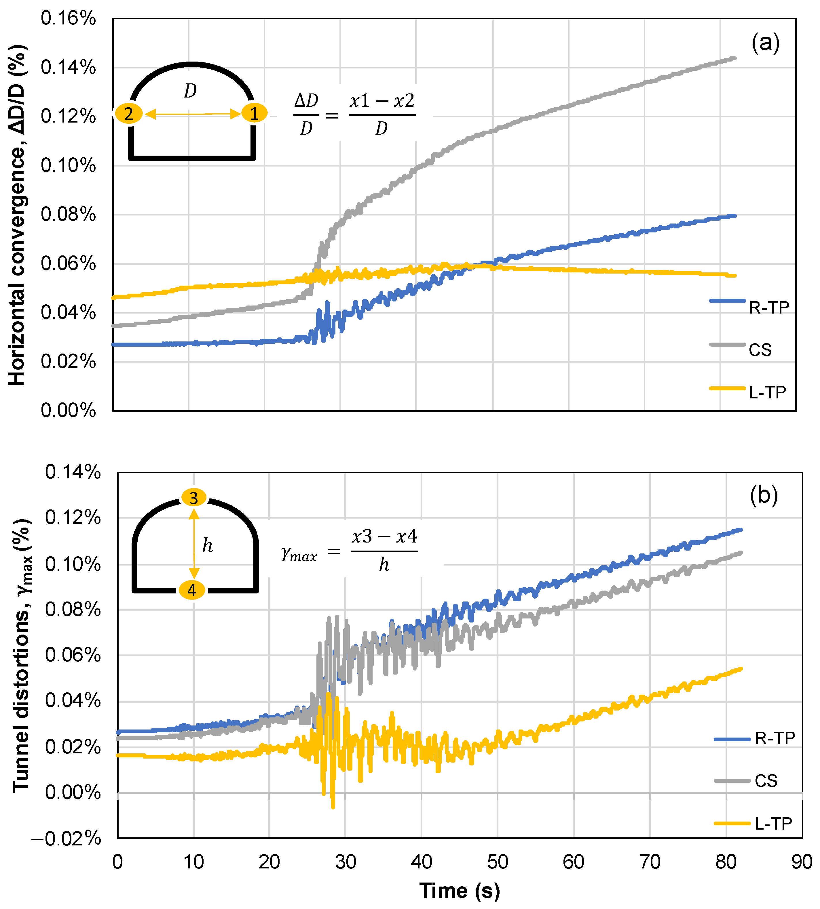
To assess the structural performance of the tunnel under seismic loading, relative displacements around the lining were obtained. For deformation in the tunnel cross-section, normalized convergences, ∆D/D, and distortions, γ_max, were calculated, and for axial and curvature deformations along tunnel longitudinal axis, maximum axial force reached during the earthquake was calculated. Figure 21 shows the corresponding results at the same cross-sections used for the slope displacement analysis. Points 1 and 2 from Figure 21 were used for the estimation of ∆D/D, and points 3 and 4 for γ_max. The results indicate that the largest seismic demand occurs at the central section, and the right tunnel portal, consistent with the zones of largest slope seismic displacements. This spatial correlation agrees with the experimental findings of Li et al. [39], who showed that the position of the lining relative to the sliding surface governs its dynamic response: linings located within or immediately above the moving mass receive the landslide thrust in addition to the seismic load, concentrating damage at the mountain-side wall, crown, and haunches, whereas deeper linings are mainly governed by seismic loads and overburden pressure. However, these conditions do not significantly represent an instability condition for the tunnel cross section, due to maximum ∆D/D being approximately 0.15%, which is lower than the limit of 1% recommended in the literature and is below the operational limit value of 1/320 given by [35].

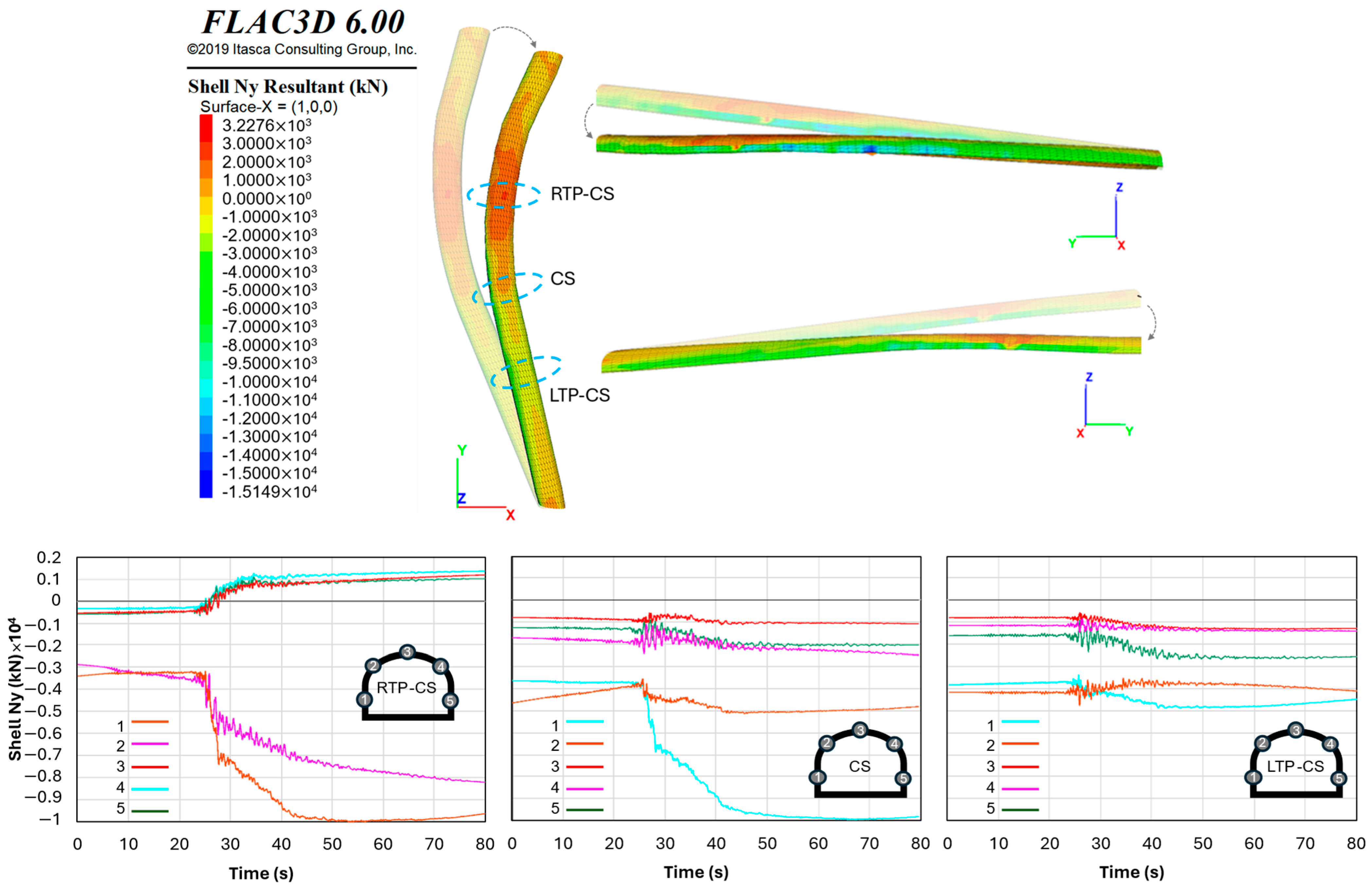
In the case of the longitudinal axis, the structural response of the tunnel lining was evaluated in terms of axial forces and correlated with the tunnel deformation after the earthquake. Figure 22 shows these deformations, identifying the three different sections considered for comparison of results where

• Between right tunnel portal, and central section (RTP-CS);
• Central section—(CS);
• Between left tunnel portal, and central section—(LTP-CS).

The solid side indicates the deformation with a scale factor of the mesh, and the thin side does not, so the deformed condition of the tunnel at the end of the seismic simulation can be appreciated. Figure 22 also shows the graphics of axial force distribution and time-history response at mentioned sections. The time response indicates that maximum compressive forces develop during the phase of greatest seismic intensity, with clear peaks observed between approximately 30 and 50 s, with a maximum axial force of ≈10 MN reached during the earthquake. This value is presented on the left wall of the lining, in the zone of maximum curvature of the tunnel, section RTP-CS. This result agrees with the seismic permanent displacements of the slope (Figure 20), since the maximum displacements occur between the right tunnel portal and the central section, which is also the zone of maximum curvature of the tunnel. On the other hand, tensile forces develop on the right wall of the lining. Such an asymmetric response is characteristic of tunnel–slope systems: Tian et al. [41] reported that, under slope deformation, the deep-buried side of the lining tends to be squeezed toward the tunnel interior while the shallow-buried side deforms outward, producing contrasting stress states on the two sides of the lining.

Regarding the other two sections, just compression stress is presented in the CS and LTP-CS zones. For the central section which has a straight alignment although both tunnel walls present compressive stresses, the left wall has similar values to those of the RTP-CS section. This can be associated with slope seismic displacements which have some influence on the tunnel’s behavior due to their proximity. Finally, in the LTP-CS zone, only compression values of lower magnitude are found because this is a straight section and is located far from the unstable zone.

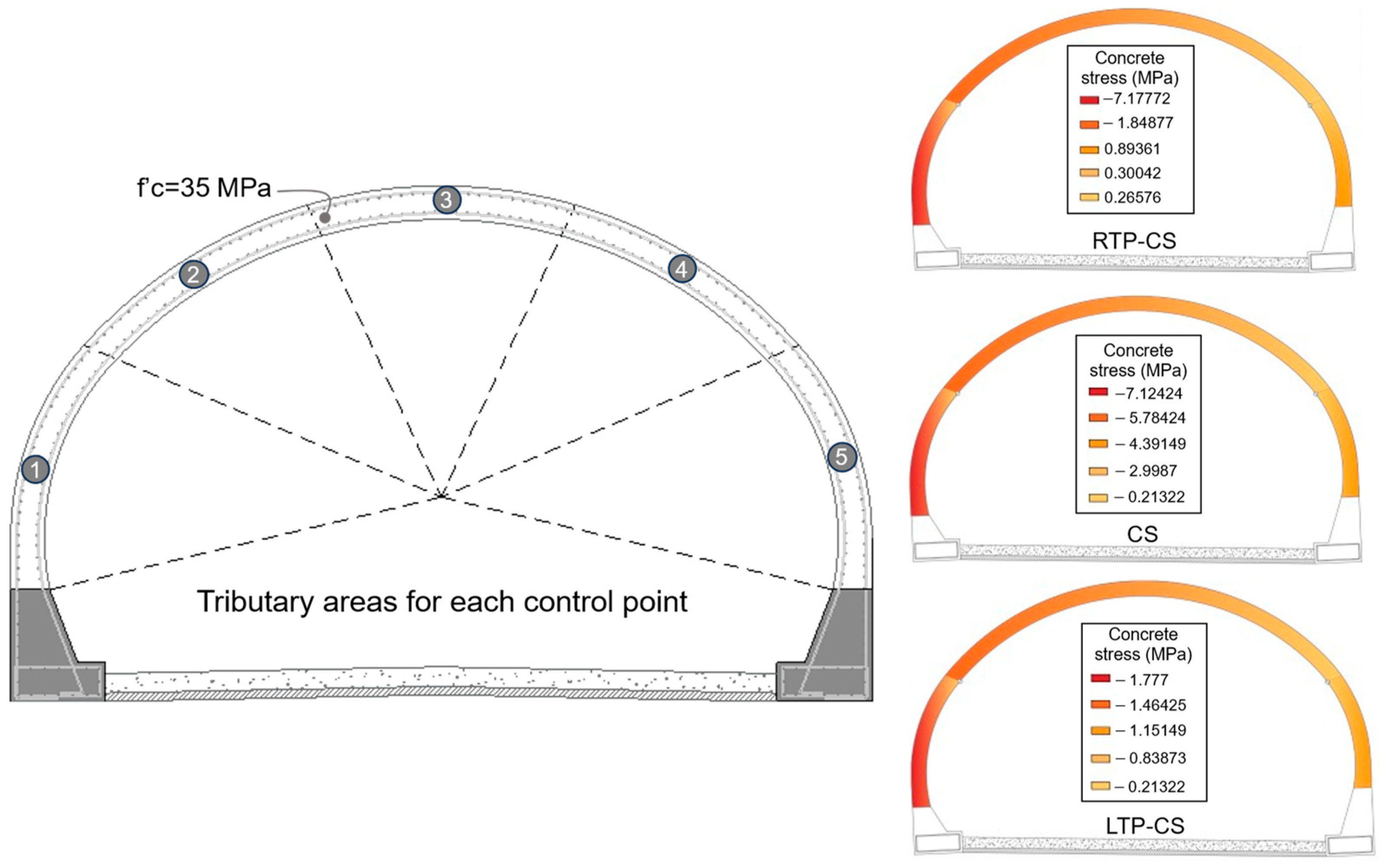
For the three sections previously evaluated (RTP-CS, CS and LTP-CS), three tributary areas were defined in order to estimate the longitudinal stresses in each section and subsequently compare them with the concrete strength to assess structural safety. The reinforcement layout and the divisions adopted to define the tributary areas are shown in Figure 23, as well as the calculated stresses.

Using the previously defined control points (Figure 22), the maximum corresponding stresses in the concrete considering their tributary areas (Figure 23) were obtained for each section. The results indicate that, at all control points, the computed stresses remain below the concrete compressive strength of f′c = 35 MPa.

In the RTP-CS section, two values indicate compressive stresses on the left side of the tunnel, while the remaining three values correspond to tensile stresses on the right side. As discussed previously, this behavior is consistent with the curvature of this section and its proximity to the slope failure zone. In contrast, for the CS and LTP-CS sections, all obtained values indicate compressive stresses across the evaluated areas.

This result demonstrates that the tunnel lining can accommodate the expected seismic deformations without compromising its structural integrity, even under the slope instability conditions present at site. Verifying the lining capacity under these combined demands is particularly relevant in light of the field evidence from the 2008 Wenchuan earthquake, where all eleven tunnels along the Dujiangyan–Wenchuan highway suffered some degree of damage, including cracking, dislocation, and local collapse of the linings, demonstrating that mountain tunnels, traditionally regarded as earthquake-resistant structures, can be severely damaged when crossing unstable slopes and weak ground [42].

In summary, in all analyzed sections, the computed stress levels remained below the adopted concrete capacity, indicating an adequate structural safety margin under the considered seismic scenario. It should be noted that this assessment addresses the global seismic performance of the lining according to established underground-structure performance criteria. Detailed crack initiation and propagation analyses, nonlinear damage models, and fatigue-related evaluations were beyond the scope of the present study. For reinforced tunnel linings, fatigue-related effects become particularly relevant under long-duration or repeated earthquake loading, or when the lining exhibits pre-existing cracks, joint defects, or material degradation, in which cases cumulative damage can sifgnificantly modify the seismic response [43,44,45,46,47]. Accordingly, local nonlinear analyses of critical curved sections, explicitly accounting for cumulative damage and fatigue effects, can be further analyzed in future research.

8. Conclusions

The performance of a tunnel–slope system in fractured rock was evaluated under static and seismic conditions for a slope that failed after intense rainfall. The observed failure was reproduced through back-analysis with strength reduction and limit equilibrium methods, and good agreement with the predicted mechanism, the documented field observations, and the phicometer measurements were obtained, which gave confidence in the calibrated geomechanical parameters. This result has practical value of its own: in projects where ground exploration is limited, the back-analysis of a documented failure provides a defensible basis to establish design parameters for three-dimensional static and seismic simulations.

Under static conditions, the interaction between the tunnel and the slope was minor. The tunneling-induced deformations were moderate, about 3.3 cm at the tunnel crown and 1.5 cm in the slope body, concentrated in the zones of lower stiffness and developed mostly in the vertical direction. The horizontal displacements, although smaller, were systematically oriented in the direction of the landslide movement; this asymmetric response is a distinctive feature of tunnel–slope systems, since under a symmetric configuration the stress redistribution caused by the excavation would produce essentially vertical movements. Regarding stability, the global safety factors remained close to 1.6 throughout construction and no global failure mechanism was formed: the low-safety-factor zones that develop around the excavation do not reach those located near the slope surface, so the interaction between both critical zones, and, therefore, the instability, does not develop, and the stability of the slope remains practically unaffected by tunneling.

Regarding the seismic evaluation, the most demanding condition for the tunnel lining was computed in the critical section where the tunnel runs closest to the unstable mass. In this zone, the lining stresses increased as a result of both the interaction with the slope and the curvature of the alignment, which produced a combined tension–compression response during the strong-motion phase of the earthquake. Even so, the diametral strains remained near 0.15%, well below the limits recommended by international standards, and the computed stresses stayed below the concrete capacity of the support.

The predicted permanent displacements, reaching approximately 70 cm under the most critical seismic scenario, indicate that the slope remains susceptible to significant deformation during strong earthquake loading. In this regard, it should be emphasized that the tunnel was not conceived to permanently stabilize the entire landslide mass, but to provide a transportation corridor that avoids direct interaction with the unstable portion of the slope by relocating the infrastructure away from the active failure zone; its effectiveness is therefore assessed in terms of tunnel stability, structural performance, and isolation from the governing landslide mechanism. Although significant seismic displacements develop within the unstable slope mass, the tunnel remains outside the critical failure zone and experiences substantially smaller deformation levels; the excavation neither triggers a new failure mechanism nor significantly increases the instability of the slope, and the support system remains within acceptable performance limits under the analyzed loading conditions. Nevertheless, the post-earthquake serviceability of the surrounding terrain and the long-term evolution of the landslide warrant further investigation, requiring additional analyses of post-seismic degradation, residual strength conditions, groundwater effects, and possible progressive deformation mechanisms, which can be further analyzed in future research.

These findings support two recommendations for practice. First, the tunnel alignment should be selected together with the slope stability assessment, not as an independent underground design problem; the favorable performance obtained here is largely explained by an alignment that stays outside the actively deforming zone and within rock of comparatively better quality. Second, the methodology applied in this study, combining back-analysis, three-dimensional simulation of the construction process, and performance-based verification of the lining, can be used to compare alternative alignments in similar projects, keeping in mind that the separation distances identified here are site-specific and should not be taken as universal design thresholds.

Finally, the main limitations of the study define complementary research lines. The fractured rock mass was represented as an equivalent continuum, which captures global deformation patterns but not cyclic degradation, damage accumulation, or discontinuity-controlled mechanisms. Future work should therefore incorporate advanced constitutive formulations and a broader range of ground motions and loading directions to further refine the assessment of tunnel performance in landslide-prone environments.