Design of a Quantitative Evaluation Framework for Highway Landscape Quality Based on Panoramic Image Segmentation

Abstract

Highway landscape quality is important for visual comfort, environmental coordination, and infrastructure management. However, conventional assessment methods rely heavily on manual inspection and qualitative judgment, which are subjective and inefficient for large-scale applications. To address this issue, this study proposes an AI-based quantitative evaluation framework for highway landscape quality using an improved Panoptic-DeepLab model for panoramic image segmentation. The model identifies major landscape elements in highway scenes, including vegetation, sky, roads, buildings, and billboards. Based on the segmentation results, the proportions of natural elements, spatial openness, and artificial interference are integrated into a landscape quality score (LQS) model for quantitative assessment. Experimental results demonstrate that the proposed method achieves reliable segmentation performance and stable convergence in complex highway environments. Comparative analysis further shows that the method provides competitive accuracy with good computational efficiency. The proposed framework offers an effective tool for highway landscape evaluation and can support highway planning, landscape optimization, and visual environment management.

1. Introduction

In recent years, intelligent algorithms have been increasingly introduced into transportation infrastructure research to support planning, operation, and decision-making processes. For example, optimization-based approaches have been applied to ship formation and route design to improve efficiency and operational performance in transportation systems. These studies indicate a broader trend toward data-driven and algorithm-assisted decision support in infrastructure engineering. However, most existing works focus primarily on operational optimization, while relatively limited attention has been paid to the quantitative evaluation of visual and environmental qualities of highway infrastructure [1]. Highway landscape space is an indispensable part of contemporary urban planning, which is meaningful for monitoring traffic conditions and highway design. Panoramic segmentation (PS) technology, as an important technology in computer vision, can classify and segment images at the pixel level. PS technology can provide strong support for the recognition and understanding of highway landscape space [2]. Despite the encouraging results achieved in highway scene segmentation and recognition, most studies have focused on improving model accuracy, while little attention has been paid to translating segmentation results into interpretable metrics for highway landscape quality assessment. Traditional PS methods have some limitations when dealing with highway landscape spaces, such as poor recognition performance for complex backgrounds and sensitivity to occlusion and lighting changes [3]. Although there are many models in PS, there are still some problems in research. Firstly, existing models require high computational resources when dealing with large-scale datasets and complex scenarios, resulting in insufficient real-time performance and scalability of algorithms [4,5]. Secondly, further improvements are needed in the adaptability to different scenarios due to the diverse characteristics and backgrounds of highway landscapes [6]. In addition, traditional dataset annotation is complex, which reduces the overall training efficiency [7,8]. To address these issues, this paper proposes a Panoptic-DeepLab PS and recognition model for highway landscape space based on a convolutional neural network (CNN). This model combines CNN and PS techniques to accurately segment and recognize different regions in the highway landscape space through deep learning and feature extraction of images. The advantages of this method in accuracy and efficiency are verified through large-scale experiments and evaluations.

The innovation of this research is mainly reflected in the proposal of an improved Panoptic-DeepLab PS recognition model based on CNN. This model integrates deep learning and PS technology. Meanwhile, advanced technologies, such as grouping convolution, deep separable convolution, deformable convolution, and attention mechanism, are utilized. This model significantly improves the recognition accuracy and adaptability of highway landscape space and effectively solves the limitations of traditional methods in complex scenes.

The contribution of this study is to provide a new method with high accuracy and precision for the automatic identification and analysis of highway landscape space. This method proves its superior performance in recognition accuracy, precision, recall, and IoU through large-scale experiments. Meanwhile, this model provides important theoretical reference and technical support for highway planning and management practices. In addition, the paper puts forward an improvement for the shortcomings of existing research, points out the direction for future research in related fields, and promotes the development and application of highway landscape spatial PS technologies.

The remainder of this paper is organized into four sections. The first is a review of the current research status of landscape recognition based on deep learning. The second is the construction of the Panoptic-DeepLab PS recognition model. The third is the evaluation and empirical study of the training effect of PS models. The fourth is to summarize the research results and provide solutions to optimize the shortcomings of the research.

2. Related Works

In recent years, image segmentation methods based on CNNs have achieved significant progress in complex scene understanding tasks and have gradually been applied to traffic infrastructure environment analysis. Ali N. et al. developed a framework called “DeepRadiation” to automatically predict urban environmental performance. The framework was trained using panoramic street-view images containing buildings, and both qualitative and quantitative evaluations demonstrated high accuracy [9]. Jiaming Z. et al. addressed the problem of unsupervised domain adaptation in panoptic semantic segmentation and proposed a general framework that achieved superior performance compared with existing methods on several benchmark datasets [10]. Hassan R. et al. proposed a deep hierarchical network based on 3D point clouds, which achieved promising results in object classification and component segmentation tasks [11]. Vinod P.V. et al. employed a CNN-based approach for urban landscape classification, achieving an overall classification accuracy of 89.65% and an F1-score of 93.03% [12]. Ashis P. et al. proposed a discontinuous contour reconnection technique to address the problem of contour discontinuity in segmented images [13]. Thomas H. et al. introduced an information-enhanced single-frame method based on instance star graphs. By integrating instance information directly into the segmentation process rather than using it as a post-processing step, the method improved segmentation efficiency and accuracy on urban landscape datasets [14].

With the rapid development of deep learning technologies, computer vision methods have also been increasingly applied to infrastructure structure recognition and condition assessment. For example, Hu Z. et al. proposed an intelligent prediction method for rock core integrity based on deep learning. In their study, semantic segmentation was used to automatically detect fissure features in rock core images, and the fissure rate was further calculated to evaluate rock core integrity. Experimental results demonstrated high accuracy in both fissure detection and integrity prediction, indicating the strong potential of deep learning-based semantic segmentation methods for infrastructure structure recognition and engineering condition assessment [15]. These studies highlight that vision-based intelligent recognition approaches can provide effective technical support for analyzing complex engineering environments.

In terms of segmentation network design, many studies have focused on improving the accuracy and efficiency of semantic segmentation models. Qingxuan L. et al. proposed a lightweight real-time segmentation model with a parallel complementary layer to enlarge the receptive field and enhance model performance [16]. Rui L. et al. developed an attention-aggregation feature pyramid network based on the feature pyramid architecture for semantic segmentation of high-resolution remote sensing images, demonstrating its effectiveness on multiple datasets [17]. Slade S. et al. introduced a particle swarm optimization-based method to optimize hyperparameters in transfer learning tasks [18]. Fengmao L. et al. improved cross-domain segmentation by leveraging image-level annotations from target images, which enhanced model adaptability across different domains [19]. Lan Y. et al. proposed a diffusion convolution network (DCNet) that combines convolutional neural networks and graph convolutional networks to improve semantic segmentation performance [20]. Zhedong Z. et al. improved pseudo-label learning by explicitly estimating prediction uncertainty, enabling dynamic confidence threshold adjustment and achieving competitive performance across multiple benchmark datasets [21].

Existing studies have mainly focused on improving segmentation accuracy, while relatively little attention has been paid to transforming segmentation results into practical indicators for highway landscape quality assessment. Although previous studies have laid a foundation for panoptic segmentation of highway landscape spaces, several challenges and limitations remain. Panoptic segmentation enables both semantic segmentation and instance segmentation to be performed within a unified framework, thereby providing a more comprehensive representation of multi-category landscape elements in road scenes. Among these approaches, Panoptic-DeepLab adopts a bottom-up segmentation strategy that does not rely on region proposal generation, resulting in a relatively simple architecture. In addition, it provides effective multi-scale feature representation and demonstrates high efficiency and stability when processing large-scale road scenes and panoramic images. Therefore, this study proposes a Panoptic-DeepLab-based panoptic segmentation recognition model to address fine-grained object recognition, complex scene adaptability, and computational efficiency in highway landscape environments, thereby promoting the development and application of panoptic segmentation techniques for highway landscape analysis.

3. Construction of Panoptic-DeepLab Panoramic Segmentation Recognition Model

Panoptic-DeepLab is a CNN-based PS model that simultaneously performs semantic segmentation and instance segmentation within a unified framework, enabling fine-grained recognition and analysis of different objects in highway landscape images. For ease of description, the PS process in this study is divided into two closely related components: (1) a semantic parsing process that generates pixel-level semantic labels, and (2) an instance information decoding process that distinguishes individual object instances. These two components share the same backbone feature extraction network and jointly accomplish PS of road scenes through a unified decoding and prediction mechanism.

3.1. Road Landscape Visual Element Recognition Based on the Semantic Parsing Process of PS

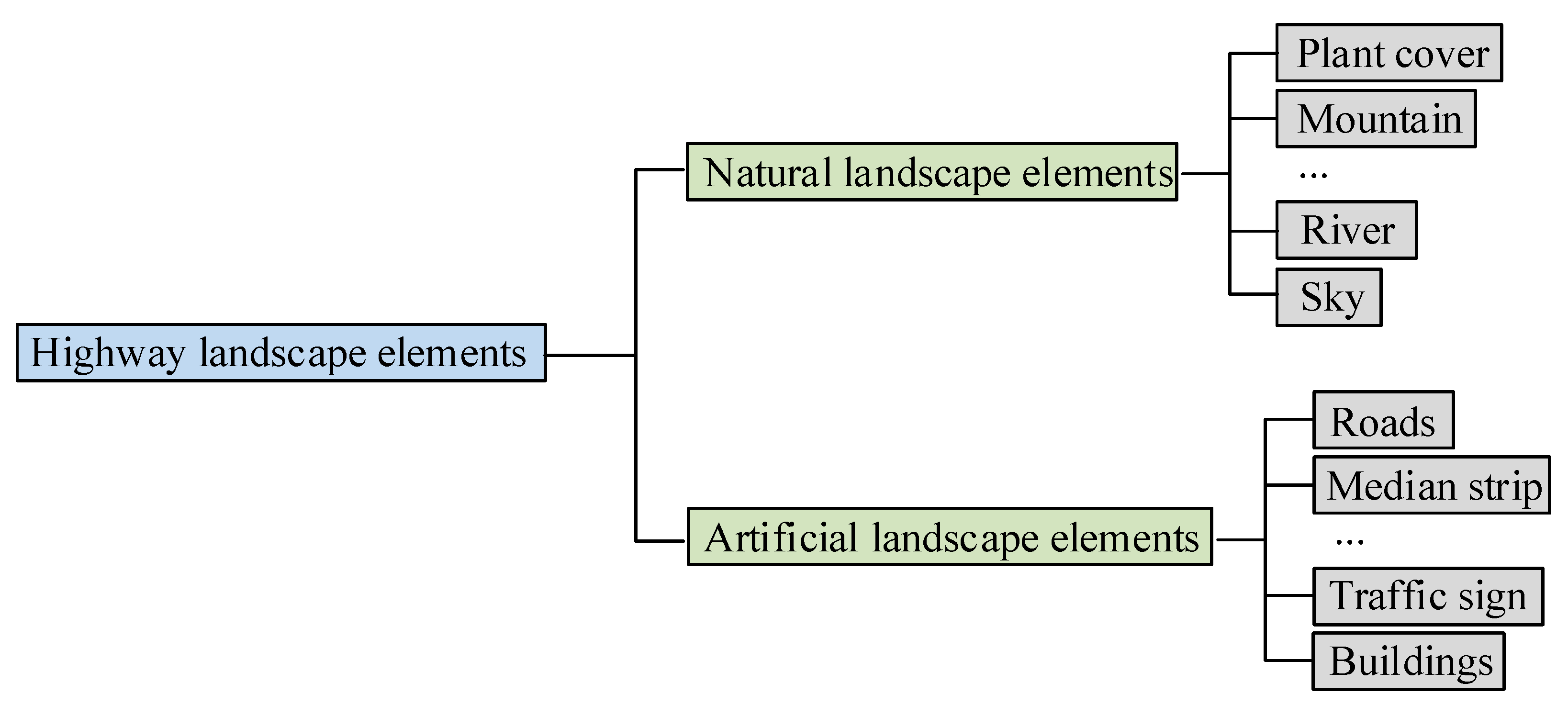
Highway landscape refers to the landscape formed by the natural environment and artificial buildings on both sides of a highway, including road surfaces, roadside greening, landscape design, transportation facilities, etc. The design and construction of highway landscapes aim to provide a beautiful, comfortable, and safe road environment, providing a pleasant visual experience for drivers and pedestrians. The scenery presented by different regions and types of highway landscapes varies, and the basic highway landscape elements are shown in Figure 1.

In Figure 1, the visual elements of a highway landscape are divided into two categories: natural and artificial. Natural landscape elements include vegetation, mountains, rivers, and sky, while artificial landscape elements include roads, isolation zones, traffic signs, and buildings. PS network is a deep learning network used to segment panoramic images into different semantic regions. Unlike traditional image segmentation tasks, PS networks segment panoramic images and can effectively extract different objects and regions from the panoramic image. PS networks typically use cross-entropy loss functions for training models, as shown in Formula (1).

$$L=-{\displaystyle \sum [y\times \log (p)+(1-y)\times \log (1-p)]}$$

(1)

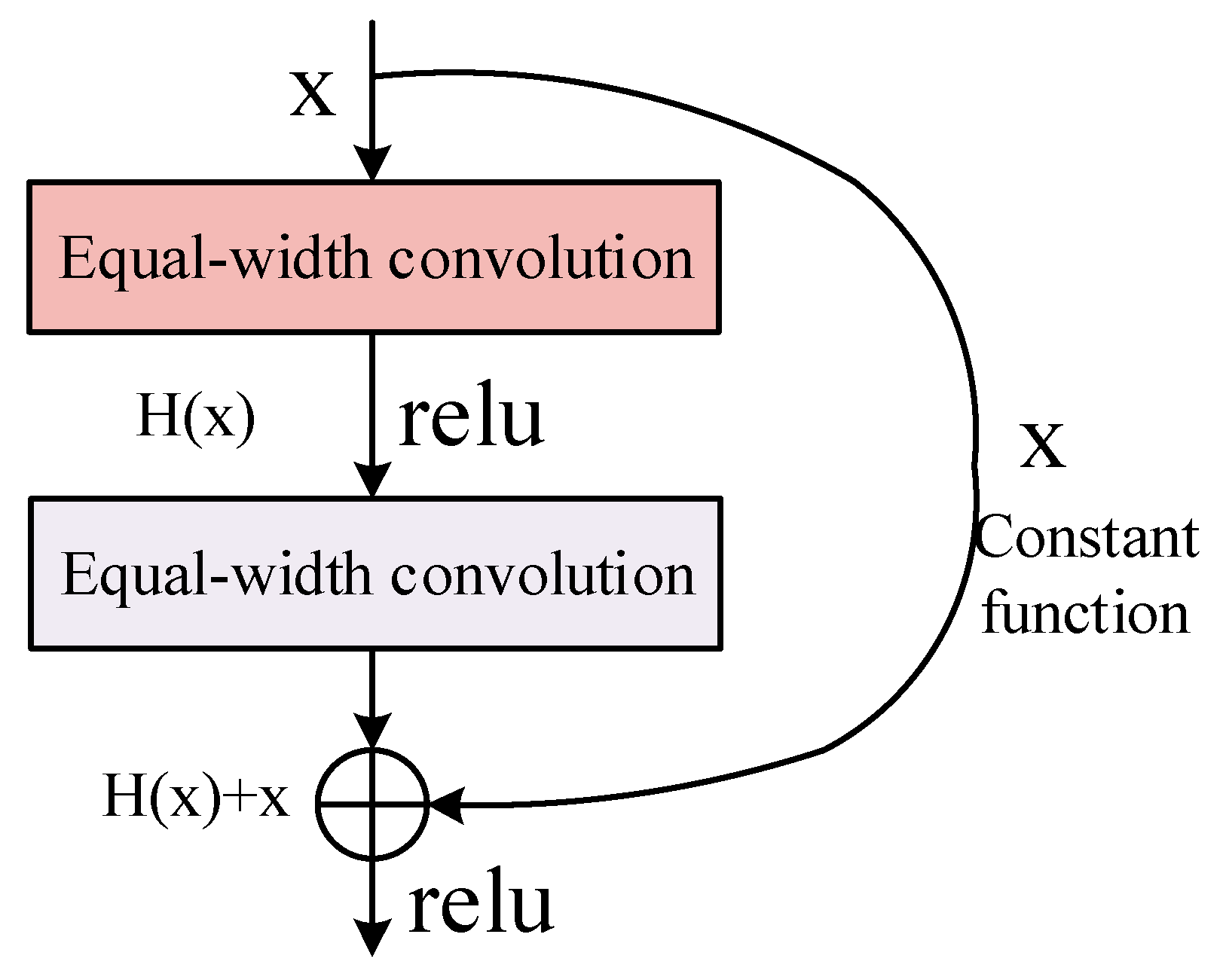
In Formula (1), $L$ serves as the loss function; $y$ serves as the true label (segmentation result); and $p$ is the probability of network prediction. In a PS network, the input is a panoramic image, which is represented by features obtained by an encoder, and then restored to its original size through a decoder to generate pixel-level segmentation results. ResNet (Residual Network) is a deep CNN architecture that introduces a “residual block” structure to enable the network to learn better representations and effectively train very deep networks. The residual unit is shown in Figure 2.

In ResNet, each residual block contains a skip connection (also known as a residual connection), introducing direct shortcuts between stacked convolutional layers, allowing information to be transmitted directly across the network. The input and output of the residual block were added and then passed through the activation function, as shown in Formula (2).

$$F(x)=H(x)+x$$

(2)

In Formula (2), $H(x)$ represents the nonlinear transformation of the residual block. The backpropagation gradient value of the ResNet network is shown in Formula (3).

$${\displaystyle \frac{\partial Loss}{\partial x}}={\displaystyle \frac{\partial F(x,w)}{\partial x}}$$

(3)

In Formula (3), $w$ is the loss value; and $F\left(x,w\right)$ serves as the loss function. The loss function of a multi-layer network is shown in Formula (4).

$$Loss=F_n\left(x_n,w_n\right)$$

(4)

In Formula (4), $n$ serves as the number of layers in the neural network. To analyze the color distribution in highway landscape images, the K-means clustering algorithm was selected for quantitative analysis of image colors. The loss function is shown in Formula (5).

$$J(c,u)=\sum _{i=1}^M{‖x_i-u_{c_i}‖}^2$$

(5)

In Formula (5), $x_i$ serves as the $i$th sample; $c_i$ serves as the cluster to which $x_i$ belongs; $u_{c_i}$ serves as the center point corresponding to the cluster; and $M$ serves as the total number of samples. The clustering effect is represented by the sum of squares of errors, as shown in Formula (6).

$$SSE=\sum _{i=1}^k\sum _{z\in C_i}{\left|p-m_i\right|}^2$$

(6)

In Formula (6), $C_i$ serves as the $i$-th cluster; $z$ serves as the sample point in $C_i$; and $m_i$ serves as the center of mass of $C_i$. The RGB (Red, Green, Blue) color mode is a light-based color mode, as shown in Figure 3.

In the feature map (FM), the color of each pixel is determined by mixing the strengths of the red, green, and blue components. When extracting pixel-level color from landscape spatial images of sample points, K-means clustering is performed using Euclidean distance to ensure the minimum color difference within the same cluster, as shown in Formula (7).

$$\Delta E=\sqrt{{\left(R_2-R_1\right)}^2+{\left(G_2-G_1\right)}^2+{(B_2-B_1)}^2}$$

(7)

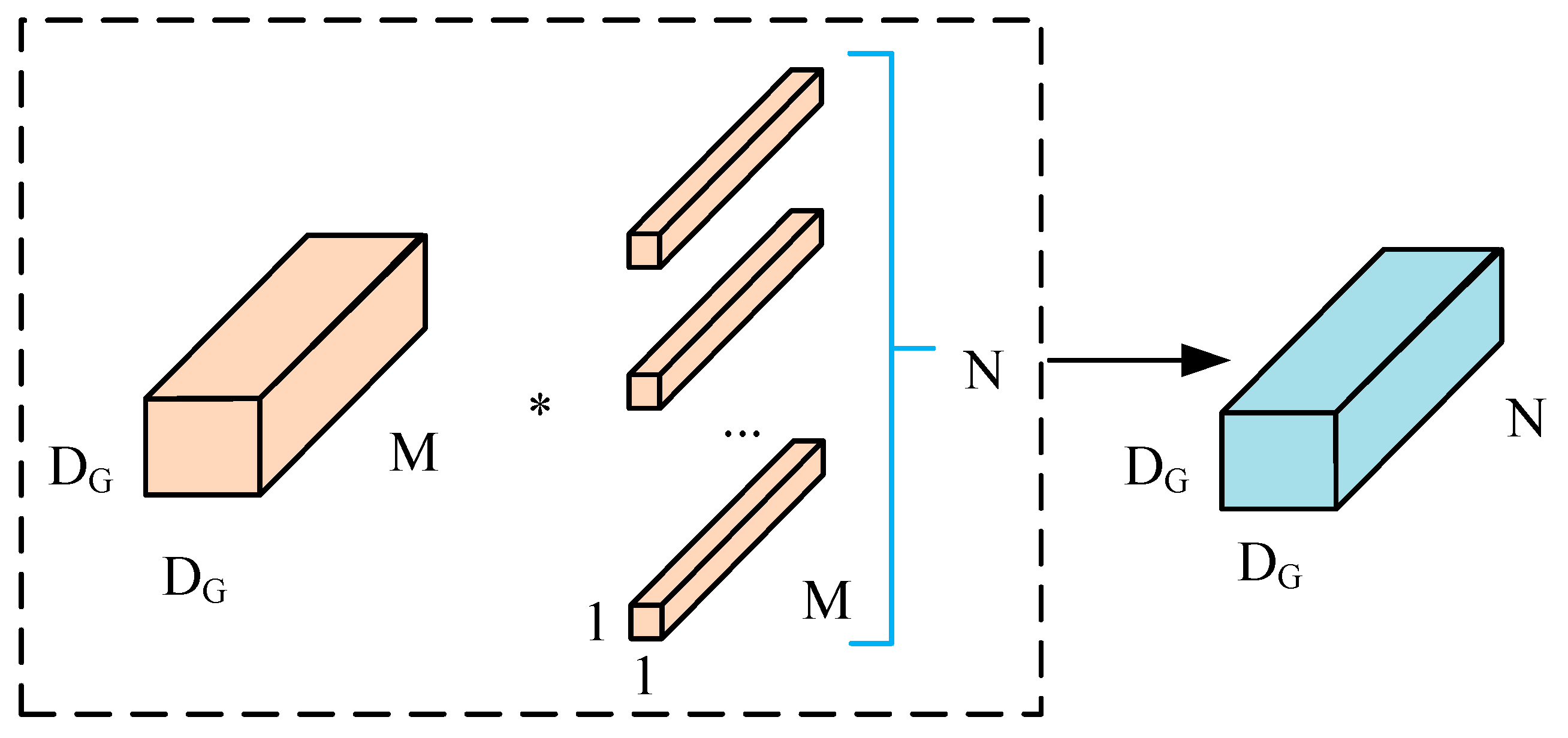
In Formula (7), $(R_1,G_1,B_1)$ and $\left(R_2,G_2,B_2\right)$ represent the RGB intensity of the colors of two pixels. In the PS network, deep separable convolution and deformable convolution are used to improve the accuracy of segmentation. Deep separable convolution is a commonly used convolution operation in CNN, which is utilized for reducing the parameters and computational complexity. The process is shown in Figure 4.

In Figure 4, the input FM size is $D_G\times D_G$, the size after separation is $1\times 1$, the accuracy before separation is $M$, and the accuracy after convolution is $N$. Each channel of the output FM is from a convolution with the corresponding input FM. For the $i$-th channel of the input FM and the $i$-th channel of the output FM, the $i$-th channel of the output FM can be calculated through a convolution operation, as shown in Formula (8).

$$ouput[i,:,:]=input[i,:,:]\ast kernel[i,:,:]$$

(8)

In Formula (8), $input[i,:,:]$ serves as the $i$-th channel of the input FM; and $kernel[i,:,:]$ serves as the corresponding convolutional kernel. We perform point-by-point convolution on the output FM of deep convolution and use 1 × 1 convolution to verify each channel for the convolution operation. In addition, attention mechanisms have been introduced to enhance the feature expression of important regions. The calculation of regional color weights is shown in Formula (9).

$$Q=a_1\ast r_1+a_2\ast r_2+\dots +a_n\ast r_n$$

(9)

In Formula (9), $Q$ represents the output representation obtained by attention weighted aggregation; $R=\left[r_1,r_2,\dots ,r_n\right]$ represents the input data characteristics; and $a=\left[a_1,a_2,\dots ,a_n\right]$ represents the attention weight of each feature $r_i$. Attention weights are generally normalized using the softmax function, as shown in Formula (10).

$$a=softmax\left(\left[e_1,e_2,\dots ,e_n\right]\right)$$

(10)

In Formula (10), $e_i$ represents the weight of feature $r_i$, which can be obtained by mapping input features using a feedforward neural network.

3.2. Road Landscape Visual Element Classification Based on Instance Information Decoding

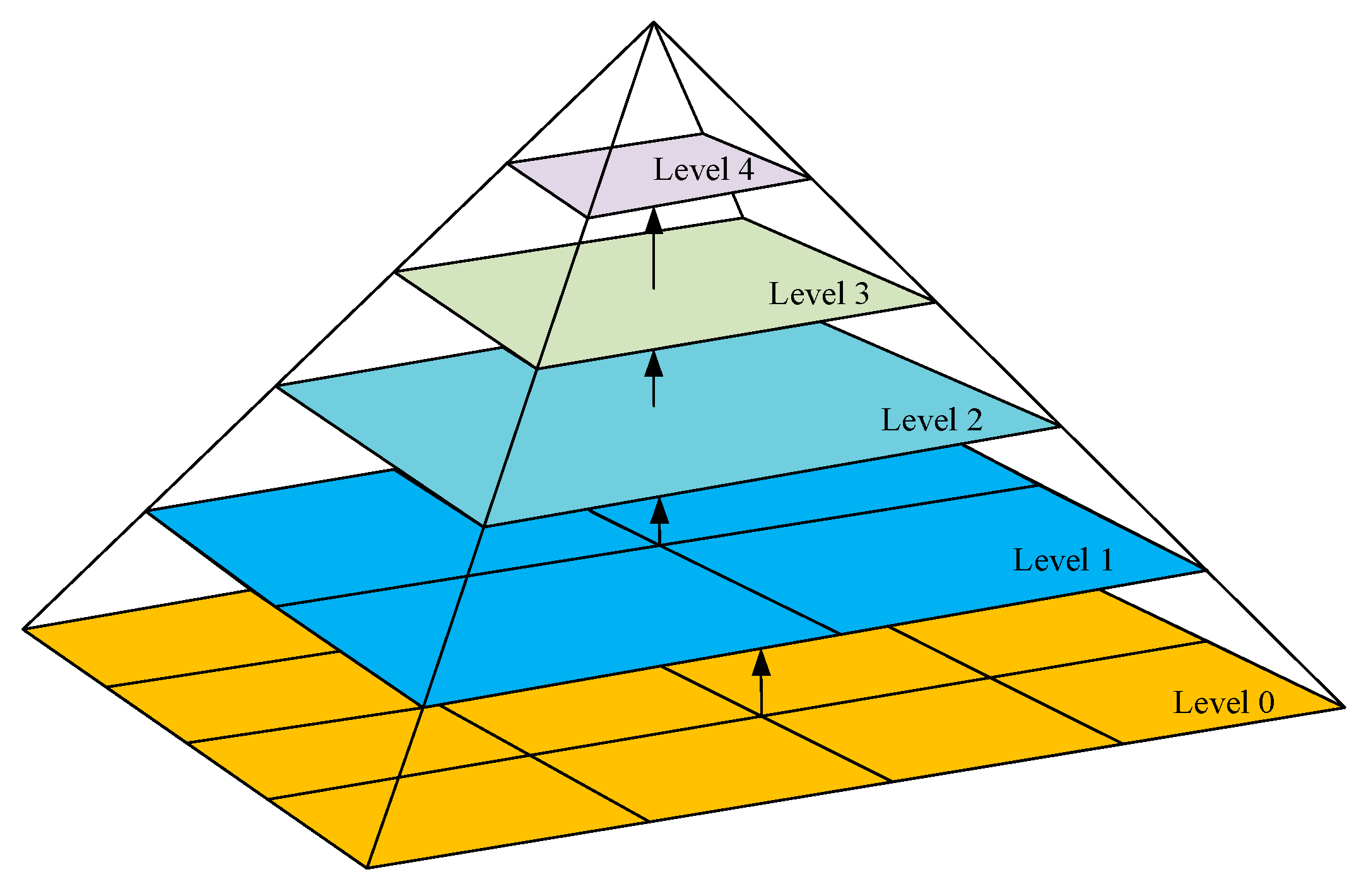
During the instance information decoding process, a top-down feature pyramid pooling strategy is adopted to fuse features at different scales. Feature pyramid pooling is commonly used in image segmentation tasks to extract multi-scale contextual information from feature matrices of different resolutions, as illustrated in Figure 5.

In Figure 5, the size of the input FM is $H\times W$; and the number of layers of the pyramid is $N$. For each pyramid layer $i(i=1,2,\dots ,N)$, the size of the FM is $H_i\times W_i$. At each layer, maximum pooling or average pooling can be used to aggregate features. Firstly, pyramid pooling of FMs is performed on each pyramid layer by using filter sizes of different sizes. The filter size of each layer is shown in Formula (11).

$$k_i=2^{\left(i-1\right)}$$

(11)

In Formula (11), $k_i$ is the filter size, where $i$ = 1, 2, N. Then, for each pyramid layer, apply maximum pooling or average pooling operations. The maximum pooling operation can be used as shown in Formula (12).

$$f_{max}\left(i,h,w\right)=max\left\{x,y\right\}\ast f\left(i, x+\left(h-1\right)\ast s, y+\left(w-1\right)\ast s\right)$$

(12)

In Formula (12), $f_{max}\left(i,h,w\right)$ represents the FM pixel after pooling the maximum value (MAX) on the pyramid layer $i$; $f\left(i, x+\left(h-1\right)\ast s, y+\left(w-1\right)\ast s\right)$ represents the original FM pixels on the pyramid layer $i$; and $s$ represents the step size on the pyramid layer $i$ (usually 2). The average pooling operation is shown in Formula (13).

$$f_{avg}\left(i,h,w\right)=mean\left\{x,y\right\}\ast f\left(i, x+\left(h-1\right)\ast s, y+\left(w-1\right)\ast s\right)$$

(13)

In Formula (13), $f_{avg}\left(i,h,w\right)$ represents the average pooled FM pixels on the pyramid layer $i$; and $mean\left\{x,y\right\}$ represents taking the average of the original feature pixels on the pyramid layer $i$. In addition, multi-scale supervision and IoU loss functions have been introduced to further improve segmentation performance. For networks with multiple scale FMs, the calculation formula for multi-scale supervision is shown in Formula (14).

$$R=w_1\ast R_1+w_2\ast R_2+\dots +w_n\ast R_n$$

(14)

In Formula (14), $w_1,w_2,\dots ,w_n$ is the weight corresponding to the FM of each scale; and $R_1,R_2,\dots ,R_n$ represents the size of different FMs. The IoU (Intersection over Union) loss function is an extensively utilized loss function for computing tasks like object detection and semantic segmentation, used to measure the degree of overlap between predicted results and real annotations. The calculation of the IoU loss function is shown in Formula (15).

$$IoU=(P\cap G)/(P\cup G)$$

(15)

In Formula (15), $P$ is given a predicted binary mask (such as the segmentation result of the target); and $G$ is the true binary mask (such as the true annotation of the target). Among them, $\cap$ represents intersection and $\cup$ represents union. The numerator serves as the area of the intersection of prediction and annotation, while the denominator serves as the area of the union of prediction and annotation. If the predicted and actual annotations completely coincide, then IoU is 1; if there is no overlap between the two, then IoU is 0. Usually, the value range of IoU is between [0, 1].

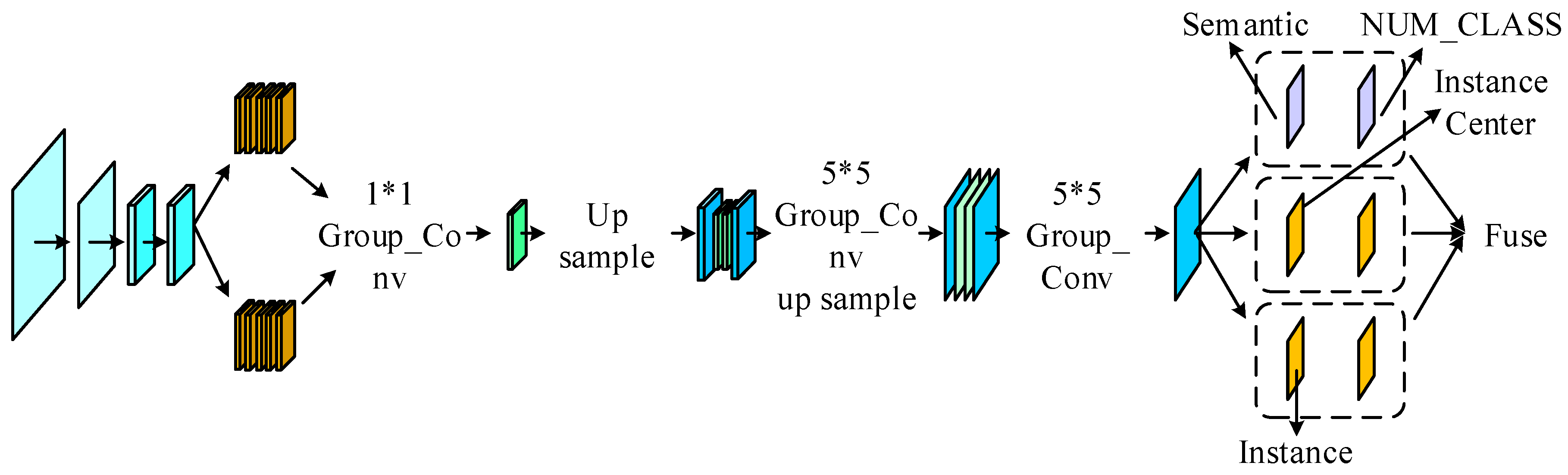
Finally, the two branches merged into a decoding network in the Panoptic-DeepLab model are prone to interfering with each other, resulting in a confusion of parameters between each other. Therefore, the paper proposes to improve the Panoptic-DeepLab model by using packet convolution assistance, and its network structure is shown in Figure 6.

As shown in Figure 6, the improved Panoptic-DeepLab model still adopts ResNet50 as the backbone network for feature extraction to obtain high-level semantic features from the input images. After the backbone network, a dual-channel atrous spatial pyramid pooling (ASPP) structure is introduced. Two parallel multi-scale context branches are used to process high-level features, enhancing feature representation under different receptive fields and improving the joint segmentation of large-scale regions and small-scale objects. In the decoding stage, the network retains two task branches, namely the semantic segmentation branch and the instance segmentation branch. Data packet convolution is employed to fuse features from different levels, enabling collaborative learning between the two tasks within a unified framework. Meanwhile, depthwise separable convolution is used to replace part of the standard convolution in the feature fusion layers, reducing the number of parameters and computational cost while improving the operational efficiency of the network. Subsequently, bilinear interpolation is used to progressively upsample the feature maps to restore spatial resolution. Finally, three prediction heads are introduced to output semantic segmentation results, instance-related features, and center point predictions, respectively, thereby achieving panoptic segmentation of different objects in road scenes. Compared with the original Panoptic-DeepLab model, the proposed architecture maintains the dual-branch panoptic segmentation framework while incorporating a dual-channel ASPP module, data packet convolution fusion, and depthwise separable convolution replacement. These modifications enhance the representation of multi-scale landscape features and improve segmentation efficiency in complex road scenes.

3.3. Highway Landscape Quality Evaluation Method

To further apply the panoramic segmentation results to highway landscape quality assessment, this paper proposes a quantitative evaluation method based on landscape composition features, building upon landscape element identification. First, an improved Panoptic-DeepLab model is used to perform pixel-level segmentation of the highway panoramic image, identifying the main visual elements in the road scene, including vegetation, sky, road, buildings, and billboards. Then, by statistically analyzing the area proportions of different landscape elements in the image, a quantitative description of the landscape structure along the highway is provided.

In highway landscape studies, natural landscape elements are generally considered to enhance the visual comfort of the road environment, while an excessive concentration of artificial facilities may interfere with the visual environment. Therefore, this paper classifies highway landscape elements into two categories based on the basic composition of the landscape visual environment: natural landscape elements and artificial landscape elements. Natural landscape elements mainly include vegetation, sky, water bodies, and mountains, while artificial landscape elements mainly include buildings, billboards, and other traffic ancillary facilities. To describe the distribution characteristics of different landscape elements in the image, the area ratio of each type of landscape element is first calculated, as shown in Equation (16).

$$P_i={\displaystyle \frac{S_i}{S}}$$

(16)

In Equation (16), $P_i$ represents the proportion of landscape elements in the image, $S_i$ represents the pixel area corresponding to this type of landscape element, and $S$ represents the total pixel area of the image. Based on this, the proportion of natural landscape elements $P_n$ and the proportion of artificial landscape elements are defined $P_a$, representing the overall proportion of natural landscapes and artificial facilities in the road scene, respectively. At the same time, the sky proportion $P_s$ is used to characterize the openness of the road space. In road landscape visual research, natural landscapes are usually considered to be the main factor affecting landscape quality, followed by the degree of spatial openness, while artificial facilities mainly manifest as visual interference. Combining relevant research and the visual environment characteristics of highways, this paper uses empirical weights for weighting. The weights of natural landscape proportion, spatial openness, and artificial interference are set to 0.5, 0.3, and 0.2, respectively, and a comprehensive landscape quality evaluation model is constructed, as shown in Equation (17).

$$LQS=0.5P_n+0.3P_s+0.2\left(1-P_a\right)$$

(17)

In Equation (17), $LQS$ represents the comprehensive landscape quality score. This model realizes a quantitative mapping from image segmentation results to landscape quality scores. The subsequent experimental section will analyze and compare the landscape quality of different road sections based on this scoring method.

4. Performance and Empirical Analysis of Panoptic-DeepLab Panoramic Segmentation Recognition Model

To evaluate the performance of the Panoptic-DeepLab PS recognition model for highway landscape space based on CNN, this study used a publicly available highway scene dataset, which contains a large quantity of highway images and corresponding annotations. The dataset has been divided into training and testing sets. The training set is utilized for model training and parameter optimization, while the test set is utilized for evaluating the model. Then, it analyzes the experimental results and compares them with other methods.

4.1. Model Training and Testing Results

The goal of Panoptic-DeepLab is to simultaneously generate semantic segmentation labels for each pixel and bounding boxes, for instance, segmentation. This means that it can recognize the category to which each pixel in the image belongs and generate a corresponding bounding box for each object to locate and segment each object in the image. To obtain the optimal model, this experiment increased the number of training iterations by 20% compared to traditional methods. The experimental environment and training parameters are showcased in

Table 1. Experimental environment and training parameters.

Experimental Environment	Hardware Parameters/or Environment Name
CPU	Xeon(R)Silver 4214@2.20GHz×24
GPU	NVIDIA GeForce RTX 3060 Ti
RAM	32G
Deep learning environment	CUDA10.2, CuDNN8.3
Open source frameworks	PaddlePaddle
Pre-training model	PaddleClas
Batch_size	4
Number of categories	12
Initial learning rate	0.01
Number of iterations	250,000

.

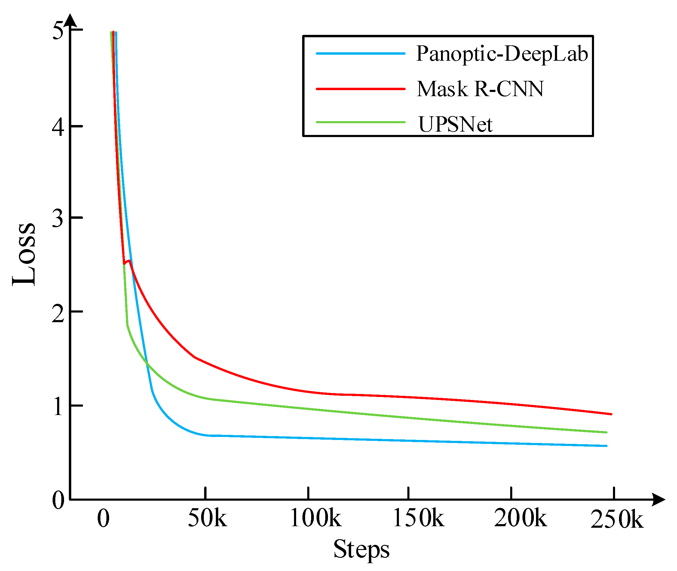
Due to the limitation of GPU memory capacity, the batch size in this study was set relatively small. Therefore, the number of training iterations was increased to improve the training performance of the model. In addition, to ensure good reproducibility of the experiments, a unified training strategy was adopted. The model was trained using the stochastic gradient descent (SGD) optimizer with a momentum coefficient of 0.9 and a weight decay of 0.0005. The input images were resized to a fixed resolution before training, and simple data augmentation techniques such as random flipping were applied to improve the generalization ability of the model. The dataset was divided into training and testing sets, where the training set was used for model parameter learning and the testing set was used for performance evaluation. All experiments were conducted under the same training configuration to ensure fairness and reproducibility of the results. The training set loss functions of different algorithms under the same parameters are shown in Figure 7.

The observation results in Figure 7 indicate that the loss functions of different algorithms continue to decrease with the increase in training times, indicating that the model gradually improves its predictive ability during the learning process, resulting in an increase in the degree of overlap between the predicted results and the actual annotations. The convergence speed of the model tends to moderate. In the initial stage, there may be significant changes in the loss value; but as the number of training increases, the model gradually stabilizes, and the trend of loss value changes slows down, indicating that the model is gradually approaching a stable state. There are differences in the convergence speed and stability loss values among the three algorithms. The convergence speed of the Panoptic-DeepLab model reaches the fastest, with a loss value stabilizing at approximately 50,000 iterations and a final stable value of 0.814. The convergence speed of the UPSNet (Unified Panoptic Segmentation Network) model is relatively slow, requiring more iterations to reach a stable state, with a stability loss value of 0.891. The convergence speed of Mask R-CNN is the slowest, and the final loss value is the highest, with a stable loss value of 1.153. Therefore, the Panoptic-DeepLab model has good performance, while the Mask R-CNN model exhibits poor performance. The research selected the segment of any 3D Gaussian (SAGA) model proposed by researchers from Shanghai Jiaotong University and Huawei in 2023, and the center focusing network (CFNet) proposed by scholars from the Beijing University of Technology in 2023 as a comparison model to verify the superiority of the model.

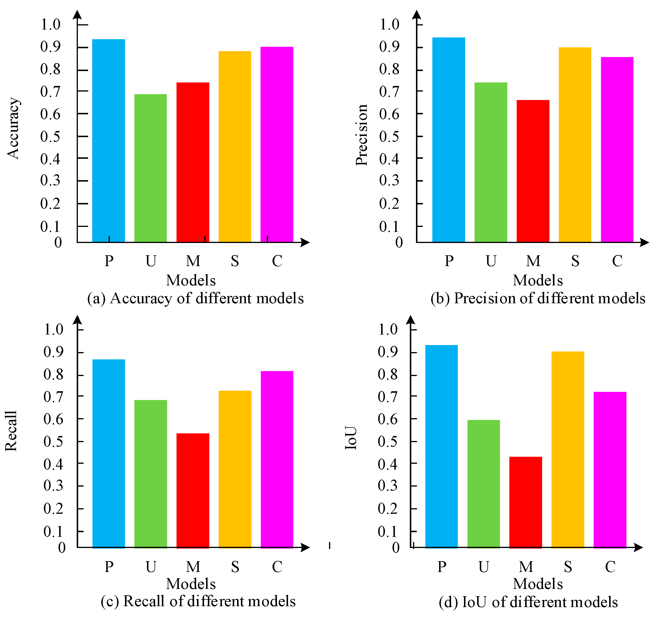
This study uses the UBGG-3m fine-grained landscape dataset, which contains street-view images collected from 36 major cities in China. The dataset includes approximately 30,000 images with a resolution of 1024 × 512, covering various road environments such as highways, urban roads, and suburban roads. Pixel-level semantic annotations are provided for 12 landscape categories, including roads, vegetation, sky, buildings, billboards, and traffic facilities. The images were captured using street-view acquisition systems under different lighting and weather conditions, providing broad geographic coverage. For model training and evaluation, the dataset was divided into training, validation, and testing subsets with a ratio of 8:1:1. The average recognition performance of different models in different scenarios is shown in Figure 8.

In Figure 8, the initials of each method are used as abbreviations. The Panoptic-DeepLab model achieves the best performance in terms of accuracy, precision, recall, and IoU, with average values of 0.934 ± 0.012, 0.963 ± 0.009, 0.884 ± 0.014, and 0.847 ± 0.011, respectively. In comparison, the UPSNet model achieves 0.683 ± 0.018, 0.744 ± 0.016, 0.657 ± 0.017, and 0.522 ± 0.019 for the four metrics. The corresponding results of the Mask R-CNN model are 0.721 ± 0.017, 0.657 ± 0.018, 0.577 ± 0.020, and 0.389 ± 0.021. In addition, both SAGA and CFNet outperform UPSNet and Mask R-CNN but remain inferior to the proposed Panoptic-DeepLab model. Overall, Panoptic-DeepLab achieves higher accuracy and stability across all evaluation metrics. 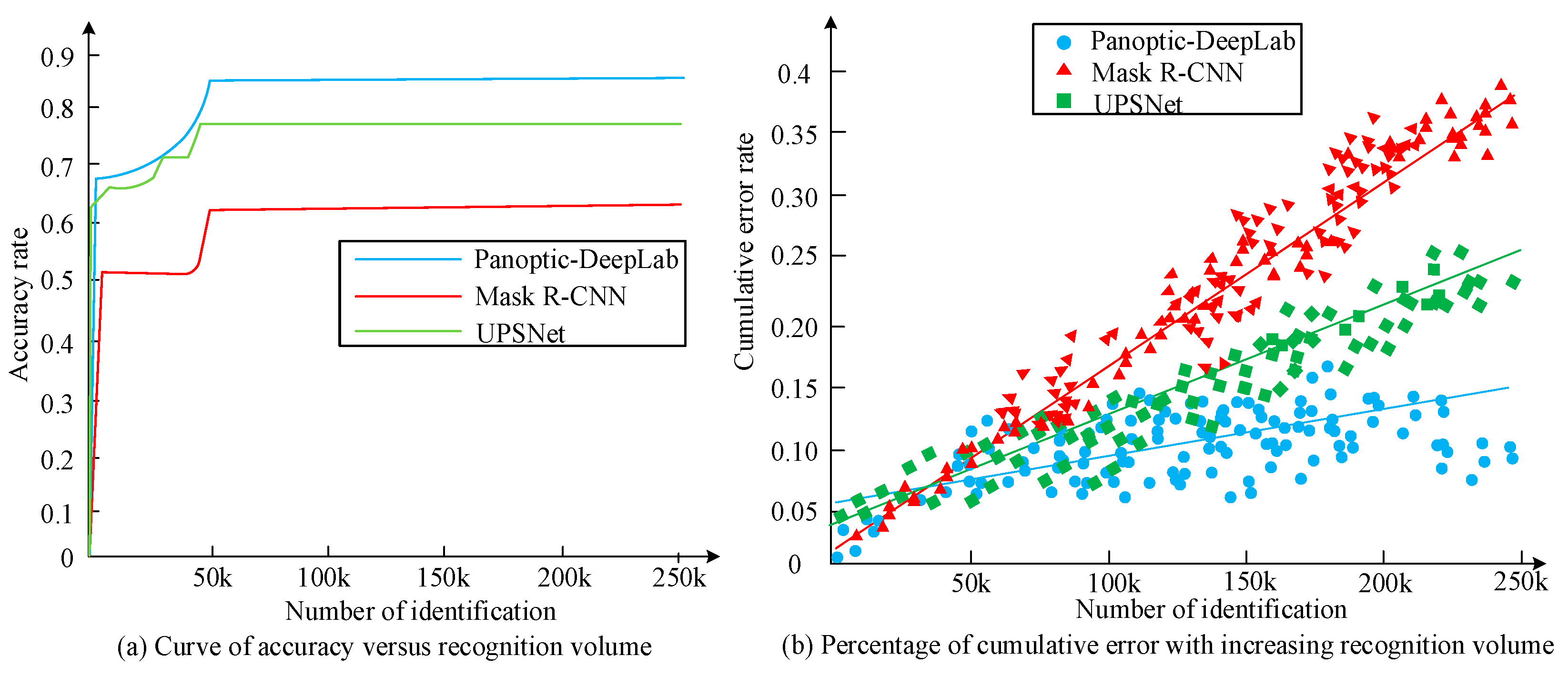Furthermore, statistical significance tests (t-test) show that the proposed method significantly outperforms the comparison models in key indicators such as accuracy and IoU (p < 0.05), demonstrating its superior performance in the PS recognition task. The recognition performance of different models on validation sets is shown in Figure 9.

Figure 9a illustrates the variation in recognition accuracy (RA) with an increase in the number of iterations. When the number of iterations approaches 50,000, the recognition accuracy of all models becomes stable. Among them, the stable RA of the Panoptic-DeepLab model reaches 0.847 ± 0.010, which is higher than that of the UPSNet model (0.774 ± 0.013) and the Mask R-CNN model (0.621 ± 0.015), indicating a stronger recognition capability in complex road scenes. Figure 9b shows the variation in cumulative recognition error rates for different models. The maximum cumulative error of the Panoptic-DeepLab model is 0.13 ± 0.008, which is significantly lower than that of UPSNet (0.24 ± 0.012) and Mask R-CNN (0.36 ± 0.015), indicating better stability during the recognition process. Further statistical analysis shows that the proposed model exhibits smaller fluctuations in both recognition accuracy and error metrics across repeated experiments, and its performance is significantly better than that of other models (p < 0.05). Therefore, the Panoptic-DeepLab model demonstrates higher stability and reliability in PS recognition tasks.

To further verify the effectiveness of the architectural improvements proposed in this study, an ablation analysis was conducted. The original Panoptic-DeepLab model with a ResNet-50 backbone was adopted as the baseline model. Based on the baseline network, three key improvement modules proposed in this study were progressively introduced, including depthwise separable convolution, an attention mechanism, and data packet convolution. All models were trained and evaluated on the same dataset using identical training settings to ensure fairness and comparability of the experimental results. The ablation results of different model structures are shown in

Table 2. Ablation study results of different model structures.

Model	Accuracy	Precision	Recall	IoU
Baseline Panoptic-DeepLab	0.903	0.921	0.861	0.823
+ Depthwise Separable Convolution	0.915	0.936	0.872	0.836
+ Attention Mechanism	0.927	0.951	0.879	0.842
+ Data Packet Convolution	0.934	0.963	0.884	0.847

.

As shown in Table 2, the baseline Panoptic-DeepLab model achieved an accuracy of 0.903 and an IoU of 0.823. After introducing the depthwise separable convolution module, the model accuracy increased to 0.915, and the IoU improved to 0.836, indicating that this lightweight convolution structure can reduce parameter redundancy while enhancing feature extraction capability. When the attention mechanism was further incorporated, the accuracy increased to 0.927, and the IoU reached 0.842, demonstrating that the attention module helps strengthen the representation of key regions and improves segmentation performance in complex scenes. Finally, after integrating the data packet convolution module, the model achieved the best performance, with an accuracy of 0.934 and an IoU of 0.847, while precision and recall also reached their highest values. Overall, the progressive introduction of the proposed modules consistently improved model performance, confirming the effectiveness of the architectural improvements proposed in this study.

4.2. Empirical Analysis of Panoptic-DeepLab Panoramic Segmentation Recognition Model

To further evaluate the segmentation performance and generalization capability of the Panoptic-DeepLab model in complex scenarios, additional experiments were conducted on the COCO dataset. The COCO dataset contains a large number of complex scenes and multiple object categories, making it suitable for assessing the model’s recognition ability in diverse visual environments.

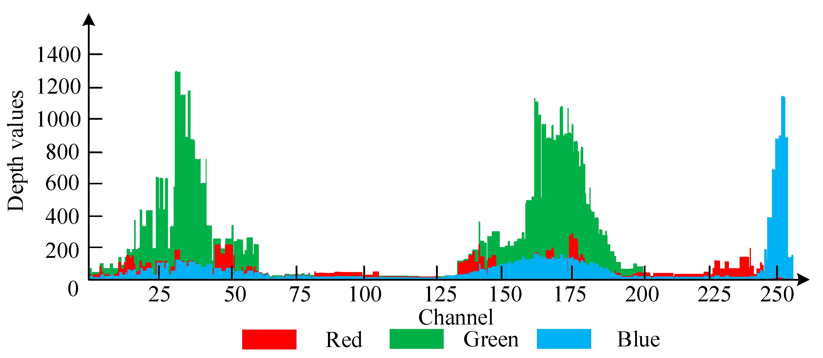
In road landscape visual studies, different color distributions usually correspond to different types of landscape elements. For example, green regions generally represent vegetation, blue regions mainly reflect sky space, while red regions are often associated with buildings, billboards, and other artificial facilities. Therefore, statistical analysis of RGB color distribution can, to some extent, reflect the spatial proportion between natural landscapes and artificial structures in road scenes. Specifically, the proportion of green typically indicates vegetation coverage, the proportion of blue reflects spatial openness, and the proportion of red indicates the density of artificial facilities. These color features can provide auxiliary information for the analysis of landscape element proportions and offer quantifiable visual characteristics for highway landscape quality assessment. Based on this analysis, the RGB color extraction results of the Panoptic-DeepLab model in complex environments are statistically analyzed, and the RGB color distribution histogram is shown in Figure 10.

Figure 10 is a histogram of RGB color extraction using the Panoptic-DeepLab model in complex environments. This indicates that the Panoptic-DeepLab model has a lower overall performance in extracting red, with higher extraction depth values in channels 0–50, 130–150, 160–180, and 225–250. For blue, the Panoptic-DeepLab model has the highest extraction depth value in the range of channels 230 to 260. For green, the Panoptic-DeepLab model has a strong overall extraction ability, with the highest extraction depth values in channels 0–60 and 150–180. The clustering color statistics in complex environments are showcased in

Table 3. Data expression of clustering colors of complex scene.

Color	Average Value	Median	Minimum Value	Maximum Value
Red	133	143	2	255
Green	147	144	21	254
Blue	157	138	1	255

.

Table 3 shows the data statistics of clustered colors in complex environments. For red colors, the average value is 133, and the median is 134. This indicates that in complex environments, the average value of red color is close to 133, and the median is close to 134. The minimum value (MIN) is 2, and the MAX is 255, demonstrating that the range of values in red is relatively wide in this environment. For green colors, the average value is 147, with a median of 144. This indicates that in complex environments, the average value of green color is close to 147, and the median is close to 144. The MIN is 21, and the MAX is 254, demonstrating that the range of values for green is relatively wide, but compared to red color, the range of values for green color is narrower. For blue colors, the average value is 157, with a median of 138. This indicates that in complex environments, the average value of the blue color is close to 157, and the median is close to 138. The MIN is 1, and the MAX is 255, indicating a relatively wide range of values for blue. In summary, red has the widest range of values with a relatively low average, while green and blue have a relatively narrow range with a relatively high average. 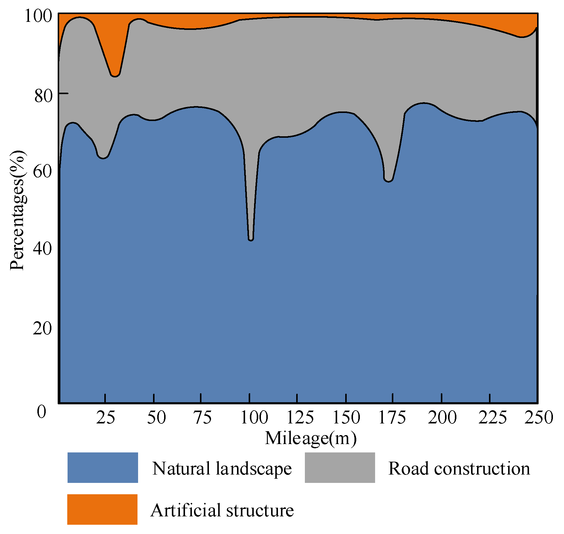The classification composition of landscape elements in a closed section of a certain highway is shown in Figure 11.

According to the classification and composition of landscape elements in the high-speed test section shown in Figure 11, it indicates that most of the natural landscape elements in the test section account for over 70%. Among them, sections 20–31 are images of village and town gathering areas, while sections 97–104 and 168–171 are locations where the overpass passes underneath, resulting in a slight decrease in natural landscape elements at these locations. The proportion of highway engineering elements remains stable at approximately 25%. Among them, 97–104 and 168–171 are mainly the locations where the overpass passes underneath, so the bridge elements have increased at these locations. The elements of artificial structures mainly include buildings and billboards. The buildings are mainly concentrated in two villages and town gathering areas, and the placement of billboards is relatively uniform. In summary, through the analysis of the classification and composition of landscape elements in the high-speed test section, it can be observed that natural landscape elements account for a relatively high proportion in most locations, while the distribution of highway engineering elements is relatively stable and uniform.

4.3. Comparison of Model Performance and Landscape Quality Evaluation Result

To further evaluate the comprehensive performance of the proposed model in terms of segmentation accuracy, computational efficiency, and landscape quality assessment, this study introduces three representative panoptic segmentation models proposed in recent years—Mask2Former, OneFormer, and kMaX-DeepLab—based on the original comparison with UPSNet and Mask R-CNN. All models were trained and tested using the same dataset, input resolution, and training strategy to ensure the fairness of the experimental comparison. The results are presented in

Table 4. Segmentation performance, computational complexity, and landscape quality evaluation result.

Model	Accuracy	Precision	Recall	IoU	Params (M)	FLOPs (G)	FPS	Mean LQS
Mask R-CNN	0.712 ± 0.018	0.651 ± 0.019	0.568 ± 0.021	0.381 ± 0.022	72.5	275.4	9.2	67.9 ± 2.5
UPSNet	0.676 ± 0.019	0.732 ± 0.017	0.645 ± 0.018	0.514 ± 0.020	63.1	248.6	10.4	71.6 ± 2.3
Mask2Former	0.901 ± 0.014	0.932 ± 0.012	0.861 ± 0.013	0.821 ± 0.013	86.3	312.8	7.6	78.2 ± 1.7
OneFormer	0.896 ± 0.015	0.928 ± 0.013	0.856 ± 0.014	0.815 ± 0.014	89.5	328.1	8.0	77.8 ± 1.8
kMaX-DeepLab	0.899 ± 0.014	0.931 ± 0.012	0.858 ± 0.013	0.818 ± 0.013	82.4	301.6	7.8	78.0 ± 1.6
Proposed method	0.918 ± 0.013	0.944 ± 0.011	0.872 ± 0.012	0.833 ± 0.012	41.8	168.3	12.1	80.3 ± 1.4

.

As shown in Table 4, compared with the traditional Mask R-CNN and UPSNet models, the recently proposed Mask2Former, OneFormer, and kMaX-DeepLab models achieve significantly higher segmentation accuracy, although their parameter sizes and computational complexity are relatively large. In contrast, the improved Panoptic-DeepLab model proposed in this study achieves the best results in terms of accuracy, precision, recall, and IoU. Meanwhile, the model contains only 41.8M parameters and requires 168.3G FLOPs, with an inference speed of 12.1 FPS. These results indicate that the introduction of depthwise separable convolution and data packet convolution effectively reduces computational complexity while maintaining high segmentation accuracy and improving operational efficiency.

It should be noted that the landscape quality evaluation model proposed in Section 3.3 is based on the results of panoptic segmentation. Specifically, the pixel area proportions of landscape elements, such as vegetation, sky, and artificial facilities, are calculated from the segmentation results to represent vegetation coverage, spatial openness, and artificial disturbance, respectively. These proportions are then combined using predefined weights (0.5, 0.3, and 0.2) to obtain the comprehensive landscape quality score (LQS). Therefore, higher accuracy, precision, recall, and IoU values indicate more accurate identification of landscape elements and smaller errors in calculating their spatial proportions, which ultimately leads to more reliable landscape quality scores.

5. Discussion

The experimental results indicate that the proposed panoptic segmentation method can reliably identify landscape elements, such as vegetation, sky, and artificial facilities, from highway panoramic images. Compared with traditional manual surveys, the proposed approach provides an objective and repeatable way to obtain landscape composition information, thereby offering quantitative data support for highway landscape quality assessment.

Based on the segmentation results, the spatial proportions of different landscape elements can be calculated to analyze landscape structure variations along different road sections. For example, in the tested highway segments, natural landscape elements occupy a relatively high proportion in most areas, whereas artificial elements such as buildings and billboards are mainly concentrated in urbanized regions and near interchanges. This spatial distribution is generally consistent with the actual road environment, indicating that the proposed method can effectively reflect variations in landscape quality along highway corridors.

In practical applications, the proposed framework can be integrated with highway monitoring systems or mobile mapping platforms. For instance, panoramic cameras mounted on inspection vehicles or mobile mapping vehicles can continuously collect road scene images, and the proposed model can automatically identify landscape elements from these images. By combining these results with the evaluation method described in Section 3.3, landscape quality scores for different road segments can be automatically calculated. In addition, the extracted information can be integrated into GIS-based infrastructure management platforms, enabling spatial visualization and management of highway landscape conditions and providing data support for highway planning, landscape improvement, and visual environment management.

It should be noted that segmentation errors may still occur in complex road environments, particularly under conditions of heavy occlusion or significant lighting variations. Future work could integrate additional data sources, such as LiDAR or multispectral imagery, to further improve the robustness of the proposed framework in complex scenarios.

6. Conclusions

This study proposes an AI-based quantitative assessment method for highway landscape quality based on an improved Panoptic-DeepLab panoramic segmentation model. This method primarily relies on automatically extracting and classifying natural and artificial landscape elements from panoramic highway images, offering better objectivity compared to traditional manual inspection methods. Comparison with various methods demonstrates that the improved model achieves stable convergence and reliable segmentation performance, accurately identifying key landscape elements even in complex highway environments. Analysis of the landscape composition of highway segments shows that natural landscape elements dominate in most segments, while artificial elements such as buildings and billboards are mainly concentrated in urban areas and near overpasses. These results are consistent with the characteristics of real highway environments, validating the effectiveness of the proposed method in landscape quality analysis. Compared to existing manual inspection and qualitative assessment methods, this model provides a more efficient and repeatable solution for highway landscape assessment. The information extracted from image segmentation results can be used for highway planning, landscape design optimization, and visual environment management, especially suitable for large or long-distance highway inspection projects, providing better theoretical support for the concept of “beautiful highway”.

References

- Xu, P.; Lan, D.; Yang, H.; Zhang, S.; Kim, H.; Shin, I. Ship Formation and Route Optimization Design Based on Improved PSO and D-P Algorithm. IEEE Access 2025, 13, 15529–15546. [Google Scholar] [CrossRef]
- Jeon, J.; Woo, A. Deep learning analysis of street panorama images to evaluate the streetscape walkability of neighborhoods for subsidized families in Seoul, Korea. Landsc. Urban Plan. 2023, 230, 104631. [Google Scholar] [CrossRef]
- Yang, H.; Xu, P.; Zhang, S.; Kim, H.; Shin, I. Construction of an intelligent analysis system for crop health status based on drone remote sensing data and CNN. IEEE Access 2025, 13, 31643–31657. [Google Scholar] [CrossRef]
- Tong, G.; Chen, H.; Li, Y.; Du, X.; Zhang, Q. Object detection for panoramic images based on MS-RPN structure in traffic road scenes. IET Comput. Vis. 2019, 13, 500–506. [Google Scholar] [CrossRef]
- Yong, H.; Huang, J.; Xiang, W.; Hua, X.; Zhang, L. Panoramic background image generation for PTZ cameras. IEEE Trans. Image Process. 2019, 28, 3162–3176. [Google Scholar] [CrossRef]
- Yang, K.; Hu, X.; Bergasa, L.M.; Romera, E.; Wang, K. PASS: Panoramic annular semantic segmentation. IEEE Trans. Intell. Transp. Syst. 2020, 21, 4171–4185. [Google Scholar] [CrossRef]
- Xu, P.; Liu, H.; Zhang, H.; Lan, D.; Shin, I. Optimizing performance of recycled aggregate materials using BP neural network analysis: A study on permeability and water storage. Desalination Water Treat. 2024, 317, 100056. [Google Scholar] [CrossRef]
- Fang, Y.; Luo, B.; Zhao, T.; He, D.; Jiang, B.; Liu, Q. ST-SIGMA: Spatio-temporal semantics and interaction graph aggregation for multi-agent perception and trajectory forecasting. CAAI Trans. Intell. Technol. 2022, 7, 744–757. [Google Scholar] [CrossRef]
- Ali, N.; Arefe, P. DeepRadiation: An intelligent augmented reality platform for predicting urban energy performance just through 360 panoramic streetscape images utilizing various deep learning models. Build. Simul. 2023, 16, 499–510. [Google Scholar]
- Zhang, J.; Ma, C.; Yang, K.; Roitberg, A.; Peng, K.; Stiefelhagen, R. Transfer beyond the field of view: Dense panoramic semantic segmentation via unsupervised domain adaptation. IEEE Trans. Intell. Transp. Syst. 2021, 23, 9478–9491. [Google Scholar] [CrossRef]
- Hassan, R.; Fraz, M.M.; Rajput, A.; Shahzad, M. Residual learning with annularly convolutional neural networks for classification and segmentation of 3D point clouds. Neurocomputing 2023, 526, 96–108. [Google Scholar] [CrossRef]
- Vinod, P.V.; Trivedi, S.; Hebbar, R.; Jha, C.S. Assessment of Trees Outside Forest (TOF) in Urban Landscape Using High-Resolution Satellite Images and Deep Learning Techniques. J. Indian Soc. Remote Sens. 2023, 51, 549–564. [Google Scholar] [CrossRef]
- Ashis, P.; Mohan, P.P. A modified Bezier curve technique for automatic reconstruction of broken contour lines extracted from a poor-quality topographic map. Multimed. Tools Appl. 2023, 82, 18299–18325. [Google Scholar]
- Hehn, T.; Kooij, J.; Gavrila, D. Fast and compact image segmentation using instance stixels. IEEE Trans. Intell. Veh. 2021, 7, 45–56. [Google Scholar] [CrossRef]
- Hu, Z.; Mei, H.; Yu, L. An intelligent prediction method for rock core integrity based on deep learning. Sci. Rep. 2025, 15, 6456. [Google Scholar] [CrossRef]
- Lv, Q.; Sun, X.; Chen, C.; Dong, J.; Zhou, H. Parallel complement network for real-time semantic segmentation of road scenes. IEEE Trans. Intell. Transp. Syst. 2021, 23, 4432–4444. [Google Scholar] [CrossRef]
- Zheng, L.; Zhou, R.; Xin, S.; Cong, H.; Qin, Y.; Xu, P.; Wang, F. Long-memory retention and self-powered ultraviolet artificial synapses realized by multi-cation metal oxide semiconductors. J. Mater. Chem. C 2023, 11, 7098–7105. [Google Scholar] [CrossRef]
- Slade, S.; Zhang, L.; Yu, Y.; Lim, C.P. An evolving ensemble model of multi-stream convolutional neural networks for human action recognition in still images. Neural Comput. Appl. 2022, 34, 9205–9231. [Google Scholar] [CrossRef]
- Lv, F.; Lin, G.; Liu, P.; Yang, G.; Pan, S.J.; Duan, L. Weakly-supervised cross-domain road scene segmentation via multi-level curriculum adaptation. IEEE Trans. Circuits Syst. Video Technol. 2020, 31, 3493–3503. [Google Scholar] [CrossRef]
- Yang, L.; Jiang, Z.; Zhou, H.; Guo, J. DCNet: Diffusion convolutional networks for semantic image segmentation. Int. J. Embed. Syst. 2021, 14, 300–311. [Google Scholar] [CrossRef]
- Zheng, Z.; Yang, Y. Rectifying pseudo label learning via uncertainty estimation for domain adaptive semantic segmentation. Int. J. Comput. Vis. 2021, 129, 1106–1120. [Google Scholar] [CrossRef]