Towards a Fair and Comprehensive Evaluation of Walkable Accessibility and Attractivity in the 15 Min City Scenario Based on Demographic Data ^†

Abstract

Accessibility and the so-called ‘15 min city’ paradigm are critical dimensions in agendas involving urban policies. However, when interested in accounting for accessibility from a formal perspective, researchers and practitioners should use pertinent indicators. Additionally, most of the indicators focus on the number of facilities reachable within a given time window, while the counterpart of the latter, i.e., as a measure of attractiveness, such as the number of users that can reach that given area, is not evaluated explicitly. In this paper, a comprehensive method able to capture accessibility and attractivity simultaneously will be presented. The formulation is based on a refinement of the gravity model. As the main input, the actual number of residents was used and included in the computation. Therefore, the resulting values of accessibility and attractivity are intended to represent the real status of different degrees of walkable accessibility in urban areas. As a test field, three Italian cities were explored. The method proposed and discussed throughout the paper is aimed at providing an operative tool for planners, as well as for private stakeholders, when they are in charge of evaluating the degree of ‘walkable’ accessibility. Furthermore, the use of open and standardized data is intended to be a main strength of the proposed methodology, as it can be easily replicated in other contexts.

1. Introduction

Accessibility and attractivity are key notions in several disciplines [1,2,3], emerging in recent decades as prominent topics of research. Measures of accessibility typically combine the costs of transport, which can be expressed either as travel distance or monetary cost or as the attractivity of the destination related to the number of activities located at the desired destination [1,4]. With regard to attractivity, the location and the density of activities at the potential destinations [3], as well as their variety and diversity in their typology [5], may influence citizens’ predispositions and habits and consequently may affect the accessibility of a place. Given their role in transportation and urban planning domains, accessibility and attractivity have been analyzed as major and critical components of the so-called ‘15 min city’ (15MC) paradigm. Several previous studies elaborated indexes and metrics to analyze the walkability of a place, and some of them are specifically devoted to analyses of the 15MC. However, the majority of these models are based on simplified representations of accessibility and attractivity. In particular, they are based on either Euclidean buffers or isochrones, rather than network-based computations. Consequently, these tools fail to consider the actual ability of people to reach their desired destinations within a reasonable amount of time.

Based on these premises, two comprehensive indicators able to capture the accessibility and the attractivity of an area will be presented and tested in three Italian cities, namely Brescia, Milano and Venezia. Methodologically, the proposed indicators are based on an enhanced version of the gravity model, which is a well-known procedure used for modeling movements of people at different spatial scales. The proposed measures include the demographic profiles of the registered population, as well as some main facilities related to the typical everyday life of most users’ categories. In particular, the actual number of residents is accessed from official sources, such as the Italian national institute of statistics (ISTAT), and then employed as the main input in the analysis. The use of the official number of residents, as well as their demographic profile, is intended to be an element of particular relevance of the proposed method. In fact, when accessibility and attractivity are considered as measures of walkability in residential areas, it is crucial to identify the actual status of the users, including their ability to reach a specific destination. Regarding the facilities, they are extracted from OpenStreetMap (OSM), a popular source of geospatial information. Results will be validated with some measures, namely the Closeness Centrality [6] and the Anselin Local Moran’s I [7], to test the ability of the metrics in unveiling the spatial patterns of accessibility and attractivity. Therefore, the proposed approach is aimed at being an operative tool for urban and transportation planners, as well as for private stakeholders, when they are in charge of evaluating the degree of ‘walkable’ accessibility within the context of the 15MC. The rest of the paper is organized as follows: Section 2 a literature review. Section 3 delves into the description of the proposed methodology, whose results are presented in Section 4 and discussed in Section 5. In the conclusive Section 6, some further possible research streams are outlined.

2. Literature Review

Several research efforts explored some aspects of accessibility and attractivity, widely regarded as comprehensive and multifaceted concepts [8,9]. With this regard, the current debate shifted the focus from mobility [10,11], namely the need to move individuals and goods [12], to accessibility, which is a derived-demand concept [12,13]. In these terms, the shift refers to a user-centered approach, with substantial relationships between transportation matters and urban planning [1,14]. Notably, the concept of accessibility is inextricably connected with equity, where the provision of adequate services is emphasized as a main prerequisite [15,16,17,18]. In accordance with this latter aspect, the definition of accessibility ranges from the ability to reach a specific location [19,20] to the focus on individuals and their freedom to satisfy trip purposes towards the desired activities [21] and the related benefits, given the economic impacts related to the access to a specific destination [22,23]. As pointed out by Geurs and Van Wee [24], several components should be simultaneously considered and combined when accounting for accessibility, including spatial, temporal, individual and transport aspects. From an operative point of view, the debate on the appropriate methodology resulted in the formulation of several measures, in relation to the components taken by the model, the level of aggregation and the spatial scale [1,4,9,10,25,26,27,28]. Most of the metrics are based on the gravity model [29] and further refinements, e.g., two-step floating catchment area (2SFCA) [30,31], able to overcome some limitations of the gravity model at specific scales [32,33,34,35].

In addition to the topics introduced above, the ‘15 min city’ (15MC) paradigm emerged during recent decades. This concept has been defined by academia [36] and gained appeal from applications and strategies put in practice in different contexts [37]. Despite the use of several time thresholds [38,39], in the domain of accessibility 15 min is still the most popular and investigated time window. From a wider perspective related to urban planning, the 15MC paradigm is rooted in the idea that different aspects of everyday life should be located in the same area and integrated, e.g., at the neighborhood level, thereby providing citizens and city users with a reasonable and adequate number of facilities related to the routine needs of people [40]. A non-exhaustive list of facilities may include both public services, such as schools, healthcare structures or banks, and commercial activities, such as restaurants, groceries or shops. In concrete terms, this assumption advocates that facilities and services should be accessible and in proximity to places of residence [5], within a travel time not exceeding 15 min [41], covered by active mobility modes, such as walking [23] or cycling [42]. In these terms, the 15MC aligns with the debates related to accessibility theoretical principles [17,18,24]. Consequently, the 15MC paradigm includes both physical and social factors. Regarding the former, the built environment [43] and land use mix [44] provide the underlying conditions towards the full implementation of the paradigm. Regarding the social factors, several authors [37,42,45,46] refer to social inclusion and demographic profile of the population as the main aspects. The latter is of paramount importance, as different socio-demographic groups may have dissimilar needs and mobility habits and behaviors, especially when focusing on walking. However, although the theoretical framework of the 15MC paradigm may appear straightforwardly implementable and measurable in any circumstances, it has been pointed out that there is a need for contextual solutions and local reinterpretations [5,38,40]. In particular, since the distribution of facilities may denote the stratified socio-economic development of a neighborhood or a city, a fair and comprehensive measure of the actual ‘walkability’ of a site requires adequate instruments that effectively combine the abovementioned dimensions related to the 15MC paradigm.

A considerable amount of research developed metrics for analyzing the walkability of a given area, with some studies specifically focusing on the 15MC. Most of them are currently available on the market, thus resulting in a set for review and comparison. The most well-known walking-related index is the WalkScore [47], which proposes a measure of proximity to facilities within a 0–100 scale. Today, it is a commercial-oriented platform, providing analyses related to the facilities reachable by walking, as well as information related to the real estate market. A main drawback is the limited performance in some countries, while it is fully implemented in the US, UK, Canada and Australia. A recent example aimed at providing a comprehensive analysis of the 15MC is the 15 min-City index proposed by Bruno et al. [40], where scores related to walkability and cycling of several cities can be accessed by a web platform. The scores are centered on a regular grid made of a hexagonal tessellation, and they refer to the number of facilities and the related travel time. An analogous scoring procedure is the 15 min City Score Toolkit elaborated by Albashir et al. [48], which is based on the intersection between isochrones pivoted to the Uber H3 hexagonal tessellation and the facilities reachable within a 15 min walking trip. Tested only in Italy, at least to the best of the authors’ knowledge, the Next Proximity Index (NEXI) [49] provides a scalable index which also considers the potential discomfort of walking accessibility. The 15 min-City index, the 15 min City Score Toolkit and the NEXI extract the list and the location of facilities from OpenStreetMap (OSM) [50].

Based on this review, it is possible to identify some commonalities between the methodologies implemented and available, such as the implementation of standardized data and the focus on the 15MC, as well as on the related notion of accessibility intended as the number of activities reachable within a specific amount of time. Nevertheless, a comprehensive review of the analytical tasks that should be addressed when accounting for accessibility in the 15MC scenarios reveal several gaps in the current literature. In particular, the different contexts require enhanced and straightforward scalability, replicability and interoperability. For example, the use of the Uber H3 hexagonal tessellation and OSM database have been demonstrated to be consistent techniques. With regard to this paper, the use of fine-grained information of the registered population, the computation of distances based on a network-based routing rather than on buffering measures and the implementation of a comprehensive method able to capture accessibility and attractivity simultaneously are aspects that have been integrated within a unique framework, thus representing a relevant methodological novelty. In fact, the emphasis on both direct and indirect measures is identified as a noteworthy innovation, as the majority of previous works focused on accessibility only.

3. Materials and Methods

3.1. Description of the Study Area

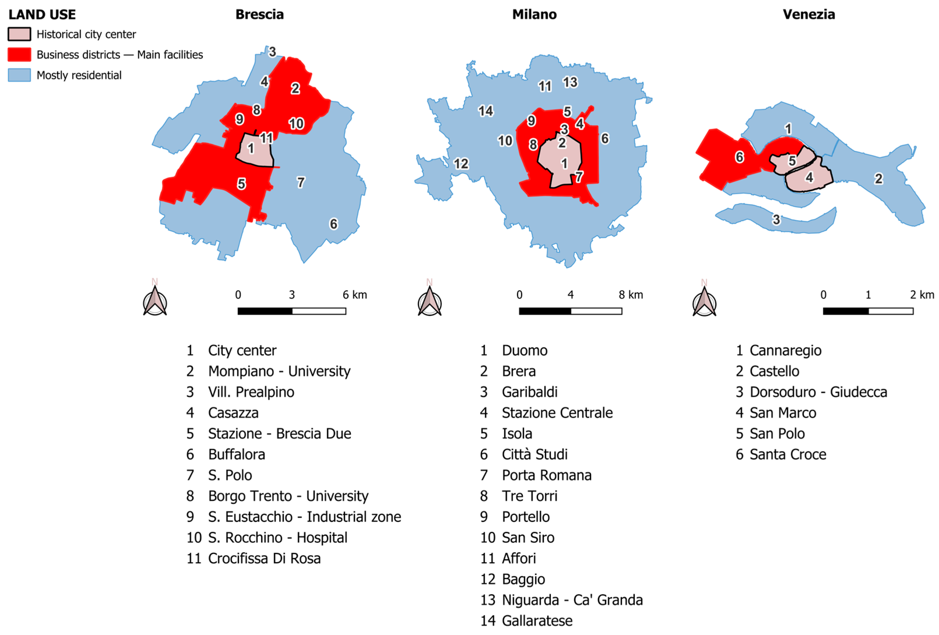
The proposed method was tested in three Italian cities, namely Brescia, Milano and Venezia. The choice of these cities is justified by their characteristics, either the size and the number of functions that may attract several categories of users (Milano and, to a lesser extent, Brescia) or the characteristics of the urban fabric that may affect the walkability (Venezia). In particular, the focus on Venezia is of particular interest, as it is a well-known pedestrian city [51,52], where the circulation of other vehicles is prohibited in most of the area, thus making it a suitable test field to evaluate the method’s suitability. Given the different socio-economic and physical backgrounds of the three test fields, Figure 1 is presented to provide readers with a comprehensive overview of the land use categories across the cities, together with a list of some notable neighborhoods and areas.

Figure 1. Notable land types and neighborhoods across the analyzed cities. Own elaboration.

3.2. Overview of the Method

In this section, the dataset employed, the analytical procedures and the metrics developed are introduced and described. From a methodological perspective, the choice of data, as well as the analytical procedures, is aimed at following the need for a thorough examination of accessibility, including the essential components identified by Geurs and Van Wee [24]. The analysis was conducted using Python 3.12, leveraging several packages for data extraction [53], tessellation [54], geospatial data analysis [55], geometric object manipulation [56] and network analysis [57]. The street network and the facilities were extracted from OpenStreetMap (OSM) [50], the largest and most successful example of a volunteered geographic information (VGI) project [58]. While the former refers to the transport component in the reference scheme [24], the latter is considered a reasonable proxy of the spatial component [24]. Despite the inherent and widely acknowledged limitations of OSM, including its non-uniform spatial coverage and the uneven characterization of information related to each spatial entity, which potentially affects the quality and reliability of the data [59,60,61], the authors opted for this source of geographic information, rather than local sources (e.g., databases provided by local authorities), to enhance the standardization of the data employed and, consequently, the replicability of the method. Moreover, a sample check was conducted to verify the correctness and the completeness of the data and address any potential issues related to data quality. Protocol buffer data for each city was downloaded from [62] and analyzed locally. Using the Pyrosm library, the walkable street network available, including sidewalks, pedestrian crossings and pedestrian zones, and the facilities have been extracted.

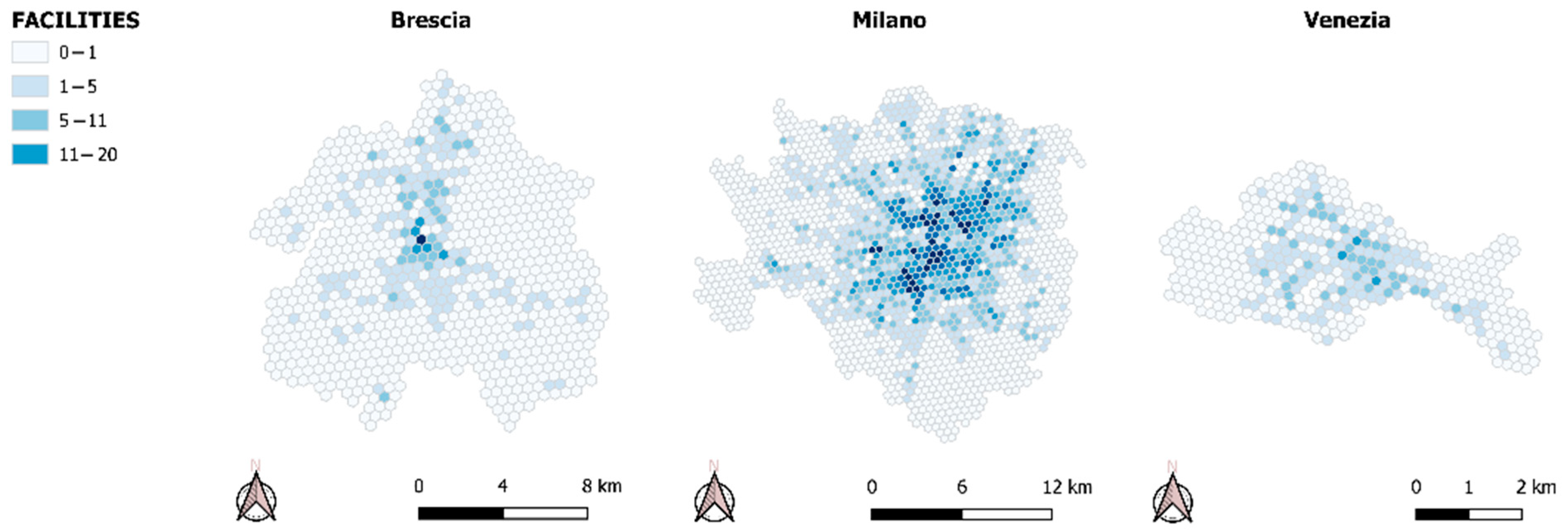
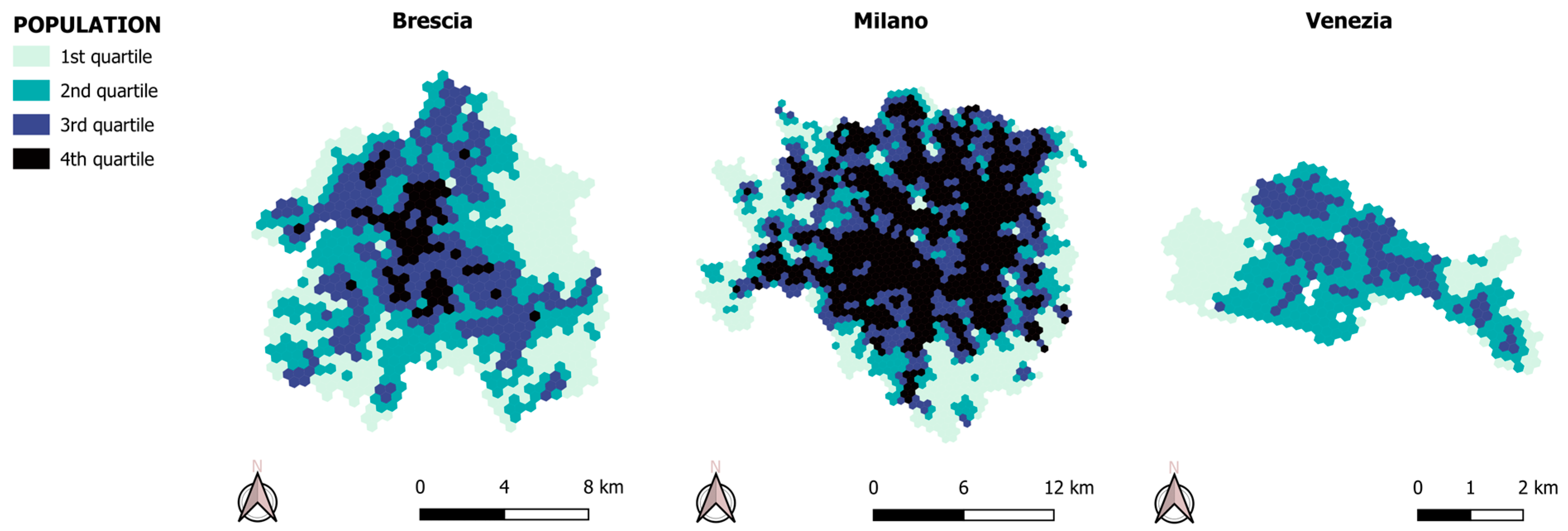
Regarding the facilities (Figure 2), the following categories were considered: restaurants, bars, schools, healthcare structures, grocery stores, parks, arts and cultural sites and banks. For each city, the official administrative delimitation layer and the Census sections were sourced from the ISTAT dataset [63], while resident population data was taken from the Italian 2021 Census [63]. Population groups, regarded as the individual component in [24], were categorized by age to assign specific walking speeds derived from Schneider [62], as described in Table 1. The implementation of different walking speeds, corresponding to the demographic composition of the population, was aimed at providing a more nuanced characterization of the potential accessibility. This approach is consistent with the granularity of analysis and the purpose of the methodology. The density of the population is plotted in Figure 3. A quartile scale has been used to allow an easier comparison between the cities analyzed.

Figure 2. Distribution of facilities. Own elaboration.

Table 1. Walking speed for each population age category group, according to Schneider [62]. The ISTAT tags are the labels used by the Italian Census for these categories [63].

Age a	ISTAT Tag	Walking Speed (m/s)
[10,11,12,13,14,15,16,17,18,19,20,21,22,23,24,25,26,27,28,29]	P-(16, 17, 18, 19)	1.34
[30,31,32,33,34,35,36,37,38,39,40,41,42,43,44,45,46,47,48,49]	P-(20, 21, 22, 23)	1.26
[50,51,52,53,54,55,56,57,58,59]	P-(24, 25)	1.23
≥60	P-(26, 27, 28, 29)	1.21

Figure 3. Distribution of population. Own elaboration.

3.3. Data Preparation

Data preparation consists of three phases: tessellation (Section 3.3.1), i.e., representing the city on a regular grid; network preparation (Section 3.3.2), i.e., cleaning OSM road network data and geometries; network matching (Section 3.3.3), i.e., assigning each facility and tessellation’s center to the closest edge of the road network.

3.3.1. Tessellation

Each of the analyzed cities was divided into a regular grid. As previously mentioned, it is based on a tessellation made up of hexagonal cells, derived from the Uber H3 scheme [64]. From a technical perspective, the resolution for Brescia and Milano was set at 9 (area: 0.10 km²; average edge length: 0.20 km), while for Venezia, it was set at 10 (area: 0.01 km²; average edge length: 0.07 km). Despite the different grid size adopted for Venezia, which was substantiated by technical reasons related to the road network described in Section 3.3.2, these schemes were regarded by the authors as pertinent spatial resolutions in analyzing accessibility at a local scale. Next, the hexagons were enriched with residential population data from the Census sections. For each hexagon in the tessellation, the Census sections intersecting it were updated and the hexagon with population information weighted by the fraction of the intersection area was identified. Specifically, let $S$ be the set of Census sections and $p\left(s,a\right)$ the resident population of age category $a$ within section $s$. The resident population of age category $a$ in tessellation $t$, denoted as $p\left(t, a\right)$, is computed as follows (Equation (1)):

$$p\left(t, a\right)={{\displaystyle \sum }}_{s\in S}{\displaystyle \frac{\mathrm{area}\left(s\cap t\right)}{\mathrm{area}\left(s\right)}}p\left(s, a\right)$$

(1)

3.3.2. Network Preparation

With this procedure, the walkable street network as a dataset comprising nodes and edges was extracted. From this dataset, a weighted graph, assigning edge weights based on street lengths in meters, was built. The tested workflow, along with the choice of libraries, allowed a significantly faster performance compared to other similar platforms [65] used elsewhere [48], particularly for shortest path computations. Furthermore, to enhance the reliability of the analysis, the most connected component $G$ of the graph and the application of a cleaning process to handle closely clustered graph components were the main focuses of this preparatory step. This method proved effective in addressing cases where OSM data contained missing edges or imprecise intersections, ensuring a more connected and accurate graph representation. Specifically, sub-graphs with at least one node within a Euclidean distance of less than 10 m from any node in the largest connected component were iteratively incorporated by creating an edge between the closest pair of nodes and assigning the Euclidean distance as the edge weight. This process continued until no remaining sub-graphs were close enough. This issue was relevant in Venezia, where the street network produced a disconnected component for Cannaregio.

Regarding the characteristics of the road network, the Closeness Centrality index [6,66] is proposed to test whether the location, the distribution and the density of nodes may have a substantial role in the computation of the metrics and hence in affecting the results described in the following Section 4. This index represents the inverse of the average distance from this node to all other nodes and was calculated with regard to each tested road network and then averaged with regard to the hexagons following Equation (2):

$$C_i^C={\displaystyle \frac{N-1}{{\sum }_{j=1; j\ne i}^N{d}_{ij}}}$$

(2)

where $N$ is the total number of nodes in the network and $d_{ij}$ is the shortest distance between nodes $i$ and $j$. Figure 4 represents the distribution of the Closeness Centrality index, where the darker the color, the higher the centrality of the related hexagon with respect to the entire city. It is worth noting that the distribution of $C_i^C$ across the study areas follows the local peculiarities, and therefore the presence of some ‘hot spots’ can be explained by the density and the characteristics of the road network.

Figure 4. Closeness Centrality. Own elaboration.

3.3.3. Network Matching

After extracting the facilities from OSM using Pyrosm and creating the tessellation, the following step involved mapping them onto the network. Each facility was represented as a point, while each tessellation was represented by its centroid. Points were dynamically integrated into the network by identifying the closest edge in $G$ for each point. Each point was then projected onto the identified edge and added as a new node in $G$, and the edge was split to accommodate the newly added node. Finally, the distance matrix was computed. For each tessellation $t$ and each facility $i_c$ of category $c$, the distance in meter $d\left(t, i_c\right)$ is computed as the shortest path distance in $G$.

3.4. Computation of the Metrics

This section is divided into subsections, namely those related to attractivity (Section 3.4.1) and accessibility (Section 3.4.3) metrics. Regarding their scope, the former is aimed at measuring the ability of each facility to attract users, while the latter measures the level of attractive facilities within a 15 min walking distance of any given area.

3.4.1. Attractivity Measures for Each Facility

An attractivity index that measures the ability to attract residents who can reach each facility within a 15 min walking distance was assigned to each potential destination. This index is a ranked statistic that compares the number of residents visiting the facility to those visiting other facilities of the same category. It was calculated separately for each population age, where the latter was categorized in accordance with the different speeds. In operative terms, this computation incorporated the speeds related to each demographic profile, as mentioned in Section 3.2.

Let $P_c$ be the set of facilities of category $c$. For any facility $i_c\in P_c$, let $T\left(i_c, a\right)$ be the set of tessellation cells from which residents of age $a$ can reach $i_c$ within 15 min. Let $p\left(i_c, a\right)= {\sum }_{t\in T}T\left(i_c, a\right)\cdot p\left(t,a\right)$ be the total number of residents of category $a$ that can reach $i_c$ within 15 min. We define the attractivity index of $i_c$ for residents of age $a$ as follows (Equation (3)):

$$\mathrm{Att}\left(i_c\right)={\displaystyle \frac{1}{\left|P_c\right|}}{\mathrm{rank}}_{P_c}\left(p\left(i_c,a\right)\right)$$

(3)

where the rank is defined as ${\mathrm{rank}}_X\left(y\right)=\left|\left\{x\in X:x\le y\right\}\right|$. For convention, equal values are associated with their minimum rank. Finally, a unique attractivity index is computed by a weighted average over the population age classes where $w\left(a\right)$ is a positive weight associated with each population category. In this analysis, uniform weights were used. This choice is substantiated by the approach adopted by the authors and described in this paper, namely testing the validity of the proposed methodology and the related net effect on the accessibility computation, which led to the implementation of a uniform weight in terms of both population category and facility. Based on the premises mentioned above, the following Equation (4) represents the attractivity measure:

$$\mathrm{Att}\left(i_c\right)=⟨\mathrm{Att}\left(i_c,a\right){⟩}_{w\left(a\right)}:={\displaystyle \frac{1}{{\sum }_{a}w\left(a\right)}}{\displaystyle \sum }_a\mathrm{Att}\left(i_c,a\right)·w\left(a\right)$$

(4)

3.4.2. Refinement Using Gravity Model

The total resident population of age a that can reach facility $i_c$ within 15 min, represented as $p\left(i_c, a\right)$, is already a valuable indicator that approximates the workload of $i_c$. However, it lacks insight into resident movements. Without relying on sensitive data and using only open-source, official information, an attractivity indicator designed to capture resident mobility was introduced. In the absence of real mobility data, movement patterns have been simulated using a refined measure based on the gravity model. This model estimates the probability of movement based on a gravity law, where the masses are the populations at the origin and destination, and the probability decreases with the square of the distance between them [29]. The total population in each tessellation cell $p\left(t\right)= {\sum }_{a}p\left(t, a\right)$ and the total population that can reach each facility within 15 min $p\left(i_c\right)= {\sum }_{a}p\left(i_c, a\right)$ were used as masses. In this regard, given the exploratory aim of the paper, the authors carefully opted for the traditional formulation of the gravity model. However, they acknowledge the potential application of other decay functions related to movements at an urban or neighborhood scale [67,68]. Thus, the probability of a movement from a tessellation cell t to a facility $i_c$ is represented by Equation (5):

$$\mathrm{Pr}\left(t,i_c\right)=k{\displaystyle \frac{p\left(t\right)·p\left(i_c\right)}{d{\left(t,i_c\right)}^2}}$$

(5)

For a normalization constant $k$. This constant can be computed by assuming that, for each tessellation, for each category of facilities and for each population age, the residents must visit at least one facility within a 15 min walk. In other words, the assumption that the residents do not walk more than 15 min was considered as a temporal constraint. In this sense, the time constraint may be considered a reasonable proxy of the time budget and hence may be considered consistent with the theoretical framework of reference [24]. Specifically, let $P_{t,c,a}$ be the set of facilities of category $c$ that population of age $a$ can reach from tessellation $t$ within 15 min. Then, following the abovementioned assumption, it is possible to formulate the following Equation (6):

$$1={\displaystyle \sum }_{i_c\in P_{t,c,a}}\mathrm{Pr}\left(t,i_c\right)\Rightarrow k_a={\left({\displaystyle \sum }_{i_c\in P_{t,c,a}}{\displaystyle \frac{p\left(t\right)·p\left(i_c\right)}{d{\left(t,i_c\right)}^2}}\right)}^{-1}$$

(6)

Meaning that a different normalization may be needed for each population age $a$. Thus, the probability of a movement of population of age $a$ from a tessellation cell $t$ to a facility $i_c$ is represented by the following Equation (7):

$$\mathrm{Pr}\left(t,i_c,a\right)={\left({\displaystyle \sum }_{j_c\in P_{t,c,a}}{\displaystyle \frac{p\left(j_c\right)}{d{\left(t,i_c\right)}^2}}\right)}^{-1}{\displaystyle \frac{p\left(i_c\right)}{d{\left(t,i_c\right)}^2}}$$

(7)

With these probabilities, the population that walks to each facility according to the model, which is defined as $p^g\left(i_c, a\right)$, can be computed. This was performed as an expected value (Equation (8)):

$$p^g\left(i_c,a\right)={\displaystyle \sum }_{t\in T\left(i_c,a\right)}p\left(t,a\right)·\mathrm{Pr}\left(t,i_{c,},a\right)$$

(8)

Which can substitute $p\left(i_c, a\right)$ to compute the attractivity index.

3.4.3. Accessibility Measures for Tessellation

The proposed measure builds on the approach elaborated by Abbiasov et al. [69], where the authors computed a weighted rank statistic for the number of facilities reachable within 15 min from each tessellation cell. In this method, this idea was adapted by integrating the attractivity index defined in the previous section. The key distinction is that the varying importance of facilities, assigning greater weight to less attractive ones to better reflect their contribution to accessibility, was accounted for. The attractivity index of a facility, which accounts for how many people can reach the facility, acts as a proxy for its workload. A lower workload is expected to correspond to better accessibility, as it is likely to translate to shorter waiting times and reduced crowding. Let $T$ be the set of all tessellation cells, the accessibility index of a tessellation cell $t$ for category of facilities $c$ and for population age $a$ is (Equation (9)):

$$\mathrm{Acc}\left(t,c,a\right)={\displaystyle \frac{1}{\left|T\right|}}{\mathrm{rank}}_T\left({\displaystyle \sum }_{i_c\in P_{t,c,a}}\left(1-\mathrm{Att}\left(i_c\right)\right)\right)$$

(9)

where the rank is calculated over the values of the summation argument for all tessellation cells and $P_{t,c,a}$ is the set of facilities of category $c$ that population of age $a$ can reach from tessellation $t$ within 15 min. The term $1-\mathrm{Att}(i_c)$ encapsulates the assumption that an increase in a facility’s attractiveness corresponds to a decrease in its accessibility. This inverse relationship arises because higher attractiveness typically leads to greater demand, thereby increasing the facility’s workload. As the workload intensifies, the facility becomes less accessible to additional users, reflecting a trade-off between desirability and availability. The key difference from Abbiasov et al. [69] is that this approach ranks facilities by their inverse attractivity, whereas their proposal counts the number of reachable facilities. As introduced in the previous section, an aggregated accessibility index can be computed as follows (Equation (10)):

$$\mathrm{Acc}\left(t\right)=⟨⟨\mathrm{Acc}\left(t,c,a\right){⟩}_{w\left(c\right)}{⟩}_{w\left(a\right)}$$

(10)

where $w\left(c\right)$ is a positive weight associated with each category of facilities. First a weighted aggregation is computed for the category of facilities and then it is computed for population age, in relation to the demographic profile and the related walking speed.

3.4.4. Unveiling Spatial Patterns of Accessibility and Attractivity: The Anselin Local Moran’s I

Given the substantial novelty of the proposed metrics, a comprehensive and extensive evaluation may be needed to test whether the results are consistent with the socio-economic characteristics of the test fields, along with the evaluation of particular and relevant spatial patterns of results. With this latter regard, the Anselin Local Moran’s $I$ is intended as an appropriate tool in the detection of specific patterns and spatial relationships, as it identifies clusters of features with similar or dissimilar values [7]. The statistic is computed as follows (Equation (11)):

$$I_i={\displaystyle \frac{x_i-\overline{X} }{S_i^2}}{\displaystyle \sum }_{j=1; j\ne i}^n{w}_{i,j}\left(x_j-\overline{X}\right)$$

(11)

where $x_i$ is an attribute for the $i$-th feature, $\overline{X}$ is the mean of the corresponding attribute and $w_{i,j}$ is the spatial weight between the $i$-th and the $j$-th features. Regarding $S_i^2$, it is computed as follows (Equation (12)):

$$S_i^2={\displaystyle \frac{{\sum }_{j=1, j\ne n }^n{\left(x_i-\overline{X}\right)}^2}{n-1}}$$

(12)

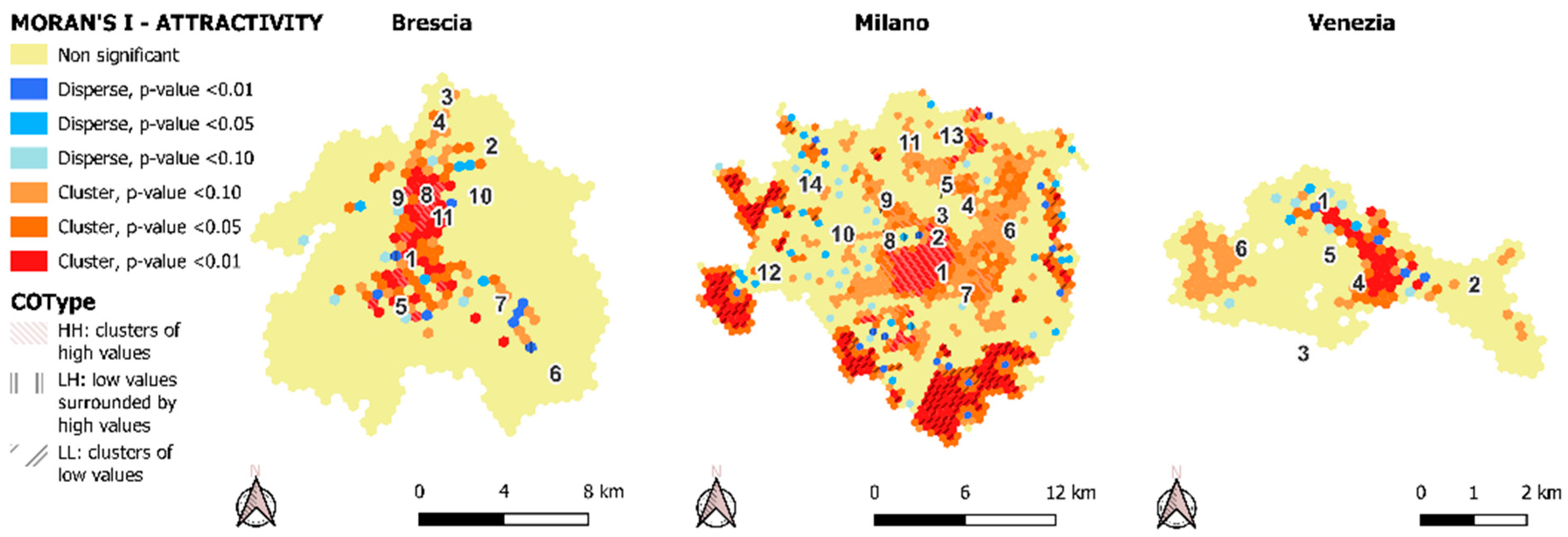
where $n$ equates to the total number of features. Regarding the visualization of the results of the computation of Anselin Local Moran’s $I$, the cluster and outlier can be plotted in accordance with the surrounding elements of each feature (COType). When $I$ is statistically significant and positive, the features are part of a cluster, while when $I$ is statistically significant and negative, the features are outliers. Conversely, when $I$ is not statistically significant, the features are randomly distributed.

4. Results

This section presents the results, while the related discussion is given in Section 5. As mentioned above, the aim of this analysis is to test and validate the effectiveness of the metrics and to unveil relevant spatial patterns related to the accessibility and attractivity across the analyzed cities. Through a correlation analysis (Pearson’s $\rho$) [70] (Table 2, Table 3, Table 4 and Table 5), results are analyzed and compared with the metrics previously introduced, namely Closeness Centrality (see Section 3.3.2) and Anselin Local Moran’s $I$ (see Section 3.4.4). As a general remark, the distribution of accessibility and attractivity values is quite similar across the cities (see Figure 5 and Figure 6). Correlations in Table 2 and Table 3 suggest that there is a notable relation between the two metrics, albeit at different degrees (Milano $\rho >0.8$, Brescia and Venezia $0.6<\rho <0.7$ all p-values $<0.001$). Along with the previous analyses, a focus on Anselin Moran’s $I$ and Closeness Centrality is proposed (Figure 7 and Figure 8) to test the spatial distribution of metrics and the effects of contextual factors, e.g., the shape of the urban fabric. The three cities report some clustering effects, albeit with different patterns, and wide areas without any significant result. However, the presence of ‘hot spots’ and ‘cold spots’ is only partially confirmed by the correlation analysis (Table 4 and Table 5).

Table 2. Correlation analysis—Accessibility (Note: *** p-value < 0.001).

	Attractivity	Population	Facilities	Centrality
Accessibility Overall	0.660 ***	0.611 ***	0.572 ***	0.391 ***
Accessibility Brescia	0.669 ***	0.690 ***	0.546 ***	0.495 ***
Accessibility Milano	0.830 ***	0.711 ***	0.639 ***	0.617 ***
Accessibility Venezia	0.626 ***	0.560 ***	0.505 ***	0.348 ***

Table 3. Correlation analysis—Attractivity (Note: *** p-value < 0.001).

	Accessibility	Population	Facilities	Centrality
Attractivity Overall	0.660 ***	0.451 ***	0.498 ***	0.169 ***
Attractivity Brescia	0.669 ***	0.583 ***	0.540 ***	0.412 ***
Attractivity Milano	0.830 ***	0.698 ***	0.534 ***	0.548 ***
Attractivity Venezia	0.626 ***	0.486 ***	0.621 ***	0.258 ***

Table 4. Correlation analysis—Anselin Moran’s I for Accessibility (Note: * p-value < 0.05; *** p-value < 0.001).

	Accessibility	Centrality
I Accessibility Overall	0.132 ***	–0.078 ***
I Accessibility Brescia	0.600 ***	0.368 ***
I Accessibility Milano	0.104 ***	–0.049 *
I Accessibility Venezia	–0.266 ***	–0.010

Table 5. Correlation analysis—Anselin Moran’s I for Attractivity (Note: * p-value < 0.05; ** p-value < 0.01; *** p-value < 0.001).

	Attractivity	Centrality
I Attractivity Overall	0.458 ***	–0.040
I Attractivity Brescia	0.549 ***	0.267 ***
I Attractivity Milano	–0.228	–0.359 **
I Attractivity Venezia	0.532 ***	0.099 *

Figure 5. Accessibility (numbers are referenced in Figure 1). Own elaboration.

Figure 6. Attractivity (numbers are referenced in Figure 1). Own elaboration.

Figure 7. Accessibility (numbers are referenced in Figure 1). Own elaboration.

Figure 8. Attractivity (numbers are referenced in Figure 1). Own elaboration.

5. Discussion

Regarding the local characteristics and spatial patterns of results, some notable findings and relationships between the metrics and the areas are worthy of further consideration. Therefore, they are discussed and referenced in accordance with the typology of land use and the name of some neighborhoods (refer to Figure 1).

Brescia was more ‘accessible’ and ‘attractive’ along an ‘L-shaped’ corridor including the neighborhoods of Prealpino, Mompiano and Casazza (refer to numbers 2, 3 and 4 in Figure 1), the historical city center, the train station and the business district of Brescia Due. As an additional remark, it is worth noting that the distribution of values is also consistent with the density of the population (refer to Figure 3; $\rho >0.5$, p-value $<0.001$), as it is possible to find specific areas characterized by high values where major residential neighborhoods, such as San Polo and Buffalora (refer to numbers 6 and 7 in Figure 1), are located. This finding is pertinent, as it suggests that accessibility and attractivity may be enhanced at the local level, thereby adhering to the 15MC paradigm. Notably, the abovementioned corridor is overlaid by the subway line, the backbone of the local transit system, thus indicating that accessibility and attractivity in Brescia are influenced by both natural and anthropic factors. The natural factors comprise geographical features, such as the hills located in the eastern part of the city, while the anthropic factors are characterized by the presence of major facilities, such as the hospital, the university campus or the business district at Brescia Due. While the former can be regarded as physical constraints that influenced the location of urban functions and facilities, the latter may have been a contributing factor in the locating activities.

As for Milano, the maps report higher accessibility and attractivity within the historical city center (Brera, Duomo; refer to numbers 1 and 2 in Figure 1), as well as the increasing values in proximity to several strategic business districts and densely populated neighborhoods (Garibaldi, Isola, Stazione Centrale, Città Studi, Porta Romana, Tre Torri, Portello; refer to numbers 3, 4, 5, 6, 7, 8 and 9 in Figure 1). The results of both metrics find correspondence with the spatial pattern that has historically characterized the urban development of Milano, namely several concentric ‘cores’ corresponding to the ancient city walls (recognizable by the red and pink background in Figure 1), with linear extensions corresponding to the main access roads. With this latter regard, the radial distribution of population (refer to Figure 3) and centrality (refer to Figure 4) can notably explain the overall correlation analyses $(\rho >0.65$ and $\rho >0.5$ respectively; both p-value $<0.001),$ positing that the corridors connecting Milano and the external areas (e.g., metropolitan region, other cities) are characterized by enhanced level of accessibility and attractivity. This lends to postulate that neighborhoods located along these corridors may benefit from local facilities and may adhere to the 15MC paradigm, though they are outside the city center.

Regarding Venezia, Figure 5 and Figure 6 suggest that the most ‘accessible’ and ‘attractive’ areas are located between San Marco and Castello (refer to numbers 2 and 4 in Figure 1), in a narrow area alongside the Canal Grande. It is worth noting that both measures overlie the most touristic areas, namely Rialto Bridge and San Marco Square, located in San Polo and San Marco (refer to numbers 4 and 5 in Figure 1). In both metrics, peripheral areas were found generally to be less ‘attractive’ and ‘accessible’ than the central areas, described in Figure 1 as the historical city centers. This finding supports the consolidated view of the city centers as the areas with a notable presence of facilities and enhanced walking capability. Results should be also regarded with specific focus on the distribution of the population, which is notably unbalanced across the city (refer to Figure 3) and clustered in specific areas, namely Cannaregio, Castello and San Polo (refer to numbers 1, 2 and 5 in Figure 1), and the specific urban fabric, as Venezia is generally considered to be a fully pedestrian-friendly city, at least in terms of its infrastructure.

In view of these trends, some insights can be discussed. Initial findings indicate that facilities are not distributed uniformly across cities, with some neighborhoods experiencing oversupply while others lack an adequate provision of services for everyday life. Consequently, the adherence to the 15MC paradigm does not necessarily follow the consolidated reputation of a city, whether being a pedestrian city or not. This is more evident in Venezia ($\rho <0.65$, p-value $<0.001$), where several populated areas are not supplied by the analyzed facilities. Consistent with the abovementioned findings, coefficients related to the population ($0.45<\rho <0.72$ p-value $<0.001$) suggest that a considerable portion of residents live in ‘fully accessible’ neighborhoods, while some of them currently need longer walks to get to the desired destinations. Consequently, results have implications for the degree to which cities conform to the 15MC paradigm, as the 15MC-based planning approach should aim to bring facilities to neighborhoods, thus promoting a more livable and functional city [38]. Furthermore, although the distribution of facilities is a determining factor in the computation of the metrics, the moderate correlation ($0.50<\rho <0.64$, p-value $<0.001$) suggests that a high concentration in some areas fosters the location of additional facilities nearby and, conversely, hinders new settlements in other areas. A similar factor was previously observed in relation to the location of economic activities and their distribution across cities [66]. This conclusion is of paramount importance for touristic destinations, as the number of facilities may be strongly skewed in favor of non-residents, while residents may suffer the lack of everyday-life facilities [71,72]. From a wider perspective, results suggest that the analysis based on the distributions of residents and facilities is effective in addressing local socio-economic dynamics [73]. This latter conclusion is corroborated when confronted with consolidated touristic patterns, such as in Venezia, as tourists’ needs may lead to inequalities and the replacement of the functions and accommodations traditionally devoted to residents [51,52,74].

Additional considerations regarding Anselin Moran’s $I$ and Closeness Centrality can be posited. While results related to Brescia are consistent, with a moderate correlation between $I$ and the two metrics ($\rho \sim 0.6$, p-value $<0.001$), Milano and Venezia report dissimilar values. Regarding the latter city, coefficients suggest that the more accessible a location, the lower its degree of clustering. Regarding Closeness Centrality, low correlations ($\rho <0.5$, p-value $<0.001$) are found with the value of the metrics, and they are weak or absent in relation to $I$. These results suggest that the structure of the road network plays a prominent role in determining the access from and to a specific area, although there are marked differences among cities, while it has no substantial effect on the spatial patterns related either to accessibility or attractivity. Nevertheless, results do not hinder particular attention being paid to the tailored improvements in accessibility and attractivity, which can range from the enhancement of road infrastructures (e.g., safe and comfortable sidewalks) to the distribution of facilities for the everyday life of residents, especially the most vulnerable categories.

6. Conclusions

In this paper, a comprehensive method tom measure accessibility and attractivity in urban areas is presented and tested in three Italian cities, namely Brescia, Milano and Venezia. The metrics are tested within the 15 min city (15MC) paradigm. Cohering with the principles the 15MC is rooted in, the socio-demographic profile of the population, the characteristics of the road network and the density of facilities for the everyday life of users are considered. Subsequently, some well-known metrics, such as Closeness Centrality and Anselin Moran’s $I$, were adopted to test the effectiveness of the results. Based on the results, the authors posit that this method provides a scalable and intuitive tool for public and private stakeholders to enhance policies aligned with the 15MC paradigm. Indeed, this paradigm aims to ensure that essential services are accessible within a short distance from residents’ homes. The use of open and standardized data sources, such as official statistics, and information from open databases facilitates informed decision making, promotes stakeholder engagement and enhances transparency and accountability in the policy-making process. Moreover, the scalability and the adherence to diverse urban contexts of the proposed method enable the development of tailored strategies that address local needs while contributing to overarching sustainability objectives, including the enhancement of public health. Furthermore, the adoption of standardized data facilitates continuous monitoring and evaluation of policy impacts, thereby instigating a continuous improvement cycle that, in turn, contributes to the creation of more resilient, equitable and habitable urban environments.

Along with the results, the authors acknowledge some limitations of the methodology in its current form. First, the analysis was restricted to the administrative limits of the cities explored. This approach may have a limited impact on accessibility in the central areas, especially when accounting for walking accessibility in the 15MC scenario, while it may have major impacts on the values exhibited by the peripheral areas. The potential distortion of results may be pronounced in conurbations or polycentric urban regions, such as the metropolitan area of Milano, where the seamless built-up areas may constitute potential destinations for residents in the areas at the edge of the core cities. This edge effect may be mitigated through the integration of additional delimitations, such as functional areas [75], rather than the use of administrative boundaries. The latter is particularly important when expanding accessibility analysis by the inclusion of other time thresholds and transport modes. In this regard, the 15 min time window may be considered a restrictive threshold when confronted with the wide spectrum of modal alternatives, which can potentially result in under- or over-representation. To address the concerns, the incorporation of transit infrastructures in a more advanced simulation model sourced by, e.g., general transit feed specification (GTFS) [76] is proposed for subsequent developments. Another relevant limitation is related to the lack of specific temporal attributes of the analyzed facilities, thereby implying their permanent availability to users. This flawed assumption may be addressed by including additional attributes related, e.g., to the actual opening hours. Addressing this limitation is expected to yield further insights into accessibility, especially in combination with the application of targeted weights following what has been mentioned in Section 3.4.1, as different categories of the population may have different needs.

Some further research may be conducted following the findings. The authors mention the shift from static, i.e., the registered population, to dynamic inputs, e.g., the number of presences inferred from big data sources. This is intended to enhance the findings and address a significant drawback related to the use of registered population data, which may be outdated and non-representative of, e.g., tourists, workers or commuters. The use of external data sources revealing the ‘real’ movements and the behaviors of the related users are also aimed at validating the current results and therefore the validity of the proposed methodology. Additionally, an approach based on the ‘real’ users may capture the effective needs of the population and the provision of adequate services. The latter has already been demonstrated to be effective for modeling dynamics in urban areas [77,78,79].

References

1. Gutiérrez, J. Transport and Accessibility. In International Encyclopedia of Human Geography; Elsevier: Amsterdam, The Netherlands, 2009; pp. 410–417. [Google Scholar] [CrossRef]
2. Nalin, A.; Fulman, N.; Wilke, E.C.; Ludwig, C.; Zipf, A.; Lantieri, C.; Vignali, V.; Simone, A. Evaluation of accessibility disparities in urban areas during disruptive events based on transit real data. Commun. Transp. Res. 2025, 5, 100160. [Google Scholar] [CrossRef]
3. Gunn, L.D.; King, T.L.; Mavoa, S.; Lamb, K.E.; Giles-Corti, B.; Kavanagh, A. Identifying destination distances that support walking trips in local neighborhoods. J. Transp. Health 2017, 5, 133–141. [Google Scholar] [CrossRef]
4. Páez, A.; Scott, D.M.; Morency, C. Measuring accessibility: Positive and normative implementations of various accessibility indicators. J. Transp. Geogr. 2012, 25, 141–153. [Google Scholar] [CrossRef]
5. Biraghi, C.A.; Ogut, O.; Dong, T.; Tadi, M. CityTime: A Novel Model to Redefine the 15-Minute City Globally Through Urban Diversity and Proximity. Urban Sci. 2025, 9, 36. [Google Scholar] [CrossRef]
6. Zheng, L.; Austwick, M.Z. Classifying station areas in greater Manchester using the node-place-design model: A comparative analysis with system centrality and green space coverage. J. Transp. Geogr. 2023, 112, 103713. [Google Scholar] [CrossRef]
7. Shekhar, S.; Xiong, H.; Zhou, X. (Eds.) Encyclopedia of GIS; Springer International Publishing: Cham, Switzerland, 2015. [Google Scholar] [CrossRef]
8. Levinson, D.M.; Wu, H. Towards a general theory of access. J. Transp. Land Use 2020, 13, 129–158. [Google Scholar] [CrossRef]
9. Wu, H.; Levinson, D. Unifying access. Transp. Res. Part D Transp. Environ. 2020, 83, 102355. [Google Scholar] [CrossRef]
10. Siddiq, F.; Taylor, B.D. Tools of the Trade?: Assessing the Progress of Accessibility Measures for Planning Practice. J. Am. Plan. Assoc. 2021, 87, 497–511. [Google Scholar] [CrossRef]
11. Levine, J. A century of evolution of the accessibility concept. Transp. Res. Part D Transp. Environ. 2020, 83, 102309. [Google Scholar] [CrossRef]
12. Levine, J.; Grengs, J.; Merlin, L.A. From Mobility to Accessibility: Transforming Urban Transportation and Land-Use Planning; Cornell University Press: Ithaca, NY, USA, 2019; ISBN 1-5017-1610-7. [Google Scholar]
13. Levine, J.; Grengs, J.; Shen, Q.; Shen, Q. Does Accessibility Require Density or Speed?: A Comparison of Fast Versus Close in Getting Where You Want to Go in U.S. Metropolitan Regions. J. Am. Plan. Assoc. 2012, 78, 157–172. [Google Scholar] [CrossRef]
14. Picard, N. What Drives Transport and Mobility Trends? The Chicken-and-Egg Problem. In International Encyclopedia of Transportation; Elsevier: Amsterdam, The Netherlands, 2021; pp. 89–94. [Google Scholar] [CrossRef]
15. Vecchio, G.; Tiznado-Aitken, I.; Hurtubia, R. Transport and equity in Latin America: A critical review of socially oriented accessibility assessments. Transp. Rev. 2020, 40, 354–381. [Google Scholar] [CrossRef]
16. Lucas, K.; Van Wee, B.; Maat, K. A method to evaluate equitable accessibility: Combining ethical theories and accessibility-based approaches. Transportation 2016, 43, 473–490. [Google Scholar] [CrossRef]
17. Van Wee, B.; Van Wee, B.; Geurs, K. Discussing Equity and Social Exclusion in Accessibility Evaluations. Eur. J. Transp. Infrastruct. Res. 2011, 11, 4. [Google Scholar] [CrossRef]
18. Ramjerdi, F. Equity Measures and Their Performance in Transportation. Transp. Res. Rec. 2006, 1983, 67–74. [Google Scholar] [CrossRef]
19. Dalvi, M.Q.; Martin, K.M. The measurement of accessibility: Some preliminary results. Transportation 1976, 5, 17–42. [Google Scholar] [CrossRef]
20. Hansen, W.G. How Accessibility Shapes Land Use. J. Am. Inst. Plan. 1959, 25, 73–76. [Google Scholar] [CrossRef]
21. Burns, L.D. Transportation, Temporal, and Spatial Components of Accessibility; Lexington Books: Lexington, MA, USA, 1979. [Google Scholar]
22. Geurs, K.T.; van Eck, J.R.R. Accessibility Measures: Review and Applications: Evaluation of Accessibility Impacts of Land-Use Transport Scenarios, and Related Social and Economic Impacts; Rijksinstituut Voor Volksgezondheid en Milieu: Bilthoven, The Netherlands, 2001. [Google Scholar]
23. Yang, L.; Wang, B.; Zhou, J.; Wang, X. Walking accessibility and property prices. Transp. Res. Part D Transp. Environ. 2018, 62, 551–562. [Google Scholar] [CrossRef]
24. Geurs, K.T.; Van Wee, B. Accessibility evaluation of land-use and transport strategies: Review and research directions. J. Transp. Geogr. 2004, 12, 127–140. [Google Scholar] [CrossRef]
25. Handy, S.L.; Niemeier, D.A. Measuring Accessibility: An Exploration of Issues and Alternatives. Environ. Plan. A 1997, 29, 1175–1194. [Google Scholar] [CrossRef]
26. Klar, B.; Lee, J.; Long, J.A.; Diab, E. The impacts of accessibility measure choice on public transit project evaluation: A comparative study of cumulative, gravity-based, and hybrid approaches. J. Transp. Geogr. 2023, 106, 103508. [Google Scholar] [CrossRef]
27. Papa, E.; Silva, C.; Te Brömmelstroet, M.; Hull, A. Accessibility instruments for planning practice: A review of European experiences. J. Transp. Land Use 2015, 9, 3. [Google Scholar] [CrossRef]
28. Silva, C.; Bertolini, L.; Te Brömmelstroet, M.; Milakis, D.; Papa, E. Accessibility instruments in planning practice: Bridging the implementation gap. Transp. Policy 2017, 53, 135–145. [Google Scholar] [CrossRef]
29. Kitchin, R.; Thrift, N. International Encyclopedia of Human Geography; Elsevier: Amsterdam, The Netherlands, 2009. [Google Scholar]
30. Javanmard, R.; Lee, J.; Kim, K.; Park, J.; Diab, E. Evaluating the impacts of supply-demand dynamics and distance decay effects on public transit project assessment: A study of healthcare accessibility and inequalities. J. Transp. Geogr. 2024, 116, 103833. [Google Scholar] [CrossRef]
31. Ni, J.; Liang, M.; Lin, Y.; Wu, Y.; Wang, C. Multi-Mode Two-Step Floating Catchment Area (2SFCA) Method to Measure the Potential Spatial Accessibility of Healthcare Services. ISPRS Int. J. Geo-Inf. 2019, 8, 236. [Google Scholar] [CrossRef]
32. Santana Palacios, M.; El-geneidy, A. Cumulative versus Gravity-based Accessibility Measures: Which One to Use? Findings 2022. [Google Scholar] [CrossRef]
33. Giannotti, M.; Tomasiello, D.B.; Bittencourt, T.A. The bias in estimating accessibility inequalities using gravity-based metrics. J. Transp. Geogr. 2022, 101, 103337. [Google Scholar] [CrossRef]
34. Simini, F.; Barlacchi, G.; Luca, M.; Pappalardo, L. A Deep Gravity model for mobility flows generation. Nat. Commun. 2021, 12, 6576. [Google Scholar] [CrossRef]
35. Barbosa, H.; Barthelemy, M.; Ghoshal, G.; James, C.R.; Lenormand, M.; Louail, T.; Menezes, R.; Ramasco, J.J.; Simini, F.; Tomasini, M. Human mobility: Models and applications. Phys. Rep. 2018, 734, 1–74. [Google Scholar] [CrossRef]
36. Moreno, C.; Allam, Z.; Chabaud, D.; Gall, C.; Pratlong, F. Introducing the “15-Minute City”: Sustainability, Resilience and Place Identity in Future Post-Pandemic Cities. Smart Cities 2021, 4, 93–111. [Google Scholar] [CrossRef]
37. Abdelfattah, L.; Deponte, D.; Fossa, G. The 15-minute city: Interpreting the model to bring out urban resiliencies. Transp. Res. Procedia 2022, 60, 330–337. [Google Scholar] [CrossRef]
38. Pozoukidou, G.; Chatziyiannaki, Z. 15-Minute City: Decomposing the New Urban Planning Eutopia. Sustainability 2021, 13, 928. [Google Scholar] [CrossRef]
39. Staricco, L. 15-, 10- or 5-minute city? A focus on accessibility to services in Turin, Italy. J. Urban Mobil. 2022, 2, 100030. [Google Scholar] [CrossRef]
40. Bruno, M.; Monteiro Melo, H.P.; Campanelli, B.; Loreto, V. A universal framework for inclusive 15-minute cities. Nat. Cities 2024, 1, 633–641. [Google Scholar] [CrossRef]
41. Allam, Z.; Bibri, S.E.; Chabaud, D.; Moreno, C. The ‘15-Minute City’ concept can shape a net-zero urban future. Humanit. Soc. Sci. Commun. 2022, 9, 126. [Google Scholar] [CrossRef]
42. Knap, E.; Ulak, M.B.; Geurs, K.T.; Mulders, A.; Van Der Drift, S. A composite X-minute city cycling accessibility metric and its role in assessing spatial and socioeconomic inequalities—A case study in Utrecht, the Netherlands. J. Urban Mobil. 2023, 3, 100043. [Google Scholar] [CrossRef]
43. Jiang, Z.; Wu, C.; Chung, H. The 15-minute community life circle for older people: Walkability measurement based on service accessibility and street-level built environment—A case study of Suzhou, China. Cities 2025, 157, 105587. [Google Scholar] [CrossRef]
44. Tsiompras, A.B.; Photis, Y.N. What matters when it comes to “Walk and the city”? Defining a weighted GIS-based walkability index. Transp. Res. Procedia 2017, 24, 523–530. [Google Scholar] [CrossRef]
45. Mitropoulos, L.; Karolemeas, C.; Tsigdinos, S.; Vassi, A.; Bakogiannis, E. A composite index for assessing accessibility in urban areas: A case study in Central Athens, Greece. J. Transp. Geogr. 2023, 108, 103566. [Google Scholar] [CrossRef]
46. Rodrigue, L.; El-Geneidy, A.; Manaugh, K. Sociodemographic matters: Analyzing interactions of individuals’ characteristics with walkability when modelling walking behavior. J. Transp. Geogr. 2024, 114, 103788. [Google Scholar] [CrossRef]
47. WalkScore. Available online: https://www.walkscore.com/ (accessed on 15 October 2025).
48. Albashir, A.; Messa, F.; Presicce, D.; Pedrazzoli, A.; Gorrini, A. 15min City Score Toolkit—Urban Walkability Analytics; Zenodo: Geneva, Switzerland, 2024. [Google Scholar]
49. Olivari, B.; Cipriano, P.; Napolitano, M.; Giovannini, L. Are Italian cities already 15-minute? Presenting the Next Proximity Index: A novel and scalable way to measure it, based on open data. J. Urban Mobil. 2023, 4, 100057. [Google Scholar] [CrossRef]
50. OpenStreetMap. 2024. Available online: https://www.openstreetmap.org (accessed on 15 October 2025).
51. Ignaccolo, C.; Zheng, Y.; Williams, S. Tourism Morphometrics in Venice: Constructing a Tourism Services Index (TSI) to unmask the spatial interplay between tourism and urban form. Cities 2023, 140, 104369. [Google Scholar] [CrossRef]
52. Bertocchi, D.; Camatti, N.; Giove, S.; van der Borg, J. Venice and overtourism: Simulating sustainable development scenarios through a tourism carrying capacity model. Sustainability 2020, 12, 512. [Google Scholar] [CrossRef]
53. Pyrosm, v0.6.2. GitHub, 2025. Available online: https://github.com/pyrosm/pyrosm (accessed on 15 October 2025).
54. Siavash-Saki. TessPy, v0.1.2. GitHub, 2025. Available online: https://github.com/siavash-saki/tesspy (accessed on 15 October 2025).
55. GeoPandas, v1.0.1. GitHub, 2022. Available online: https://github.com/geopandas/geopandas (accessed on 15 October 2025).
56. Shapely, v2.0.6. GitHub, 2024. Available online: https://github.com/shapely/shapely (accessed on 15 October 2025).
57. Csárdi, G.; Nepusz, T. The igraph software package for complex network research. InterJ. Complex Syst. 2006, 1695. Available online: https://igraph.org (accessed on 15 October 2025).
58. Capineri, C.; Rondinone, A. Geographie (in) volontarie. Riv. Geogr. Ital. 2011, 118, 555–573. [Google Scholar]
59. Herfort, B.; Lautenbach, S.; Porto De Albuquerque, J.; Anderson, J.; Zipf, A. A spatio-temporal analysis investigating completeness and inequalities of global urban building data in OpenStreetMap. Nat. Commun. 2023, 14, 3985. [Google Scholar] [CrossRef] [PubMed]
60. Grinberger, A.Y.; Schott, M.; Raifer, M.; Zipf, A. An analysis of the spatial and temporal distribution of large-scale data production events in OpenStreetMap. Trans. GIS 2021, 25, 622–641. [Google Scholar] [CrossRef]
61. Tockner, L.; Herfort, B.; Lautenbach, S.; Zipf, A. Corporate mapping in OpenStreetMap—Shifting trends in global evolution and small-scale effects. Geo-Spat. Inf. Sci. 2025, 1–20. [Google Scholar] [CrossRef]
62. Schneider, W. Extract BBBike. Available online: https://extract.bbbike.org (accessed on 1 May 2025).
63. ISTAT. Basi Territoriali e Variabili Censuarie. Available online: https://www.istat.it/notizia/basi-territoriali-e-variabili-censuarie/ (accessed on 1 May 2025).
64. Uber. Uber H3. 2025. Available online: https://h3geo.org (accessed on 15 October 2025).
65. Networkx. GitHub, 2025. Available online: https://github.com/networkx/networkx (accessed on 15 October 2025).
66. Porta, S.; Strano, E.; Iacoviello, V.; Messora, R.; Latora, V.; Cardillo, A.; Wang, F.; Scellato, S. Street Centrality and Densities of Retail and Services in Bologna, Italy. Environ. Plan. B Plan. Des. 2009, 36, 450–465. [Google Scholar] [CrossRef]
67. Šveda, M.; Madajová, M.S. Estimating distance decay of intra-urban trips using mobile phone data: The case of Bratislava, Slovakia. J. Transp. Geogr. 2023, 107, 103552. [Google Scholar] [CrossRef]
68. Martínez, L.M.; Viegas, J.M. A new approach to modelling distance-decay functions for accessibility assessment in transport studies. J. Transp. Geogr. 2013, 26, 87–96. [Google Scholar] [CrossRef]
69. Abbiasov, T.; Heine, C.; Sabouri, S.; Salazar-Miranda, A.; Santi, P.; Glaeser, E.; Ratti, C. The 15-minute city quantified using human mobility data. Nat. Hum. Behav. 2024, 8, 445–455. [Google Scholar] [CrossRef]
70. Washington, S.P.; Karlaftis, M.G.; Mannering, F.L.; Washington, S.; Mannering, F. Statistical and Econometric Methods for Transportation Data Analysis. In Statistics; Chapman & Hall/CRC: Boca Raton, FL, USA, 2003. [Google Scholar]
71. Anguera-Torrell, O.; Cerdan, A. Which commercial sectors coagglomerate with the accommodation industry? Evidence from Barcelona. Cities 2021, 112, 103112. [Google Scholar] [CrossRef]
72. Zanini, S. Tourism pressures and depopulation in Cannaregio: Effects of mass tourism on Venetian cultural heritage. J. Cult. Herit. Manag. Sustain. Dev. 2017, 7, 164–178. [Google Scholar] [CrossRef]
73. Novy, J.; Colomb, C. Urban tourism as a source of contention and social mobilisations: A critical review. Travel Tour. Age Overtourism 2021, 16, 6–23. [Google Scholar]
74. Nalin, A.; Cameli, L.; Pazzini, M.; Simone, A.; Vignali, V.; Lantieri, C. Unveiling the Socio-Economic Fragility of a Major Urban Touristic Destination through Open Data and Airbnb Data: The Case Study of Bologna, Italy. Smart Cities 2023, 6, 3138–3160. [Google Scholar] [CrossRef]
75. Dijkstra, L.; Poelman, H.; Veneri, P. The EU-OECD Definition of a Functional Urban Area; OECD: Paris, France, 2019. [Google Scholar]
76. Google. GTFS Static Overview. 2024. Available online: https://developers.google.com/transit/gtfs (accessed on 15 October 2025).
77. Nalin, A.; Simone, A.; Lantieri, C.; Cappellari, D.; Mantegari, G.; Vignali, V. Application of cell phone data to monitor attendance during motor racing major event. The case of Formula One Gran Prix in Imola. Case Stud. Transp. Policy 2024, 18, 101287. [Google Scholar] [CrossRef]
78. Zhang, Y.; Zhong, W.; Wang, D.; Lin, F.-T. Understanding the spatiotemporal patterns of nighttime urban vibrancy in central Shanghai inferred from mobile phone data. Reg. Sustain. 2021, 2, 297–307. [Google Scholar] [CrossRef]
79. Sevtsuk, A.; Ratti, C. Does Urban Mobility Have a Daily Routine? Learning from the Aggregate Data of Mobile Networks. J. Urban Technol. 2010, 17, 41–60. [Google Scholar] [CrossRef]
Disclaimer/Publisher’s Note: The statements, opinions and data contained in all publications are solely those of the individual author(s) and contributor(s) and not of MDPI and/or the editor(s). MDPI and/or the editor(s) disclaim responsibility for any injury to people or property resulting from any ideas, methods, instructions or products referred to in the content.
Article Metrics
Citations
Article Access Statistics
Article metric data becomes available approximately 24 hours after publication online.