1. Introduction
In cold regions, ice accretion on overhead transmission lines poses a significant threat to power grid stability, often inducing severe wind-excited oscillations such as galloping. These dynamic instabilities, exacerbated by aerodynamic forces acting on ice-coated conductors, can lead to catastrophic failures, including conductor breakage and tower collapse [
1,
2,
3]. Mitigating such risks necessitates a comprehensive understanding of the aerodynamic behavior of iced conductors, particularly for multi-bundled configurations employed in ultra-high-voltage (UHV) transmission systems. While extensive research has focused on single and lower-bundled conductors, the aerodynamic complexities of eight-bundled conductors—a common configuration in modern UHV lines—remain inadequately explored, especially regarding the influence of stranded geometry on simulation accuracy and wake interactions [
4,
5,
6]. Addressing this gap is critical for advancing predictive models and ensuring the operational safety of power infrastructure in ice-prone environments.
Current methodologies for analyzing iced conductors primarily integrate wind tunnel experiments and numerical simulations. Wind tunnel tests provide high-fidelity aerodynamic data under turbulent flow conditions, while computational fluid dynamics (CFD) enable cost-effective exploration of flow fields and parametric variations [
7,
8,
9]. Recent studies have advanced the understanding of iced conductor aerodynamics: For instance, numerical analyses of D-shaped and crescent-shaped iced conductors reveal significant dependencies of lift and drag coefficients on wind angles of attack [
10,
11]. Experimental work by Lou [
12] highlights the destabilizing effects of rough ice surfaces, while Liao [
13] quantified the impacts of ice thickness and wind speed using Reynolds-averaged Navier–Stokes (RANS) models. However, existing research predominantly simplifies conductor geometry to smooth surfaces, neglecting the inherently stranded structure of real-world conductors. This oversimplification introduces substantial errors in aerodynamic predictions, particularly for multi-bundled systems where wake interference between sub-conductors amplifies instability risks [
14,
15,
16]. Recent efforts by Cai [
17] and Zhou [
18] on six- and eight-bundled conductors underscore the need for high-fidelity geometric modeling, yet the role of stranded geometry in modulating aerodynamic coefficients and vortex-shedding patterns remains unresolved.
Despite these advances, a clear understanding of how stranded geometry affects both force coefficients and wake characteristics is still missing. The previous literature often focuses on either simplified models or limited bundle configurations, leaving a gap in accurate prediction for iced multi-bundled conductors under realistic conditions. In particular, the combined effects of stranded surface and ice accretion on instability mechanisms such as Den Hartog-type galloping have rarely been quantified. In this context, the present work provides a systematic investigation into the aerodynamic behavior of crescent-shaped iced eight-bundled conductors, explicitly modeling stranded geometry in both wind tunnel tests and CFD simulations. For the first time, detailed comparisons between stranded and smooth conductor models are performed to assess their impact on force prediction, wake development, and oscillation thresholds. This approach enables a more accurate evaluation of the mechanisms leading to galloping in modern UHV transmission lines. Thus, the aim and novelty of this study are to bridge the gap between idealized and realistic modeling, and to offer a validated framework for predicting and mitigating aerodynamic instability in iced multi-bundled conductors. The contributions and addressed gaps are now stated more explicitly, helping readers to better understand the advancement beyond previous work.
2. Materials and Methods
2.1. Test Material
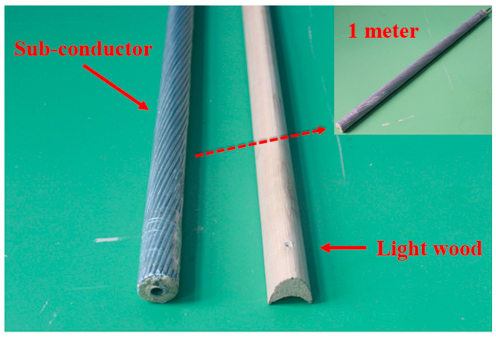
Crescent-shaped ice commonly forms on ultra-high voltage (UHV) transmission lines. The wind tunnel test model of the sub-conductor is shown in
Figure 1. The tested sub-conductor (LGJ-500/35, from Chengdu, Sichuan, China) consists of a core made of seven steel strands, each 2.50 mm in diameter. Surrounding the core are 45 aluminum strands, each with a diameter of 3.75 mm, arranged in three layers. The sub-conductor has an outer diameter of 30 mm, and the spacing between adjacent units is 400 mm. A 1 m segment of the actual conductor was modeled. In this test, real ice was replaced by lightweight wood with a density similar to that of ice. The specific parameters of the conductor are shown in
Table 1.
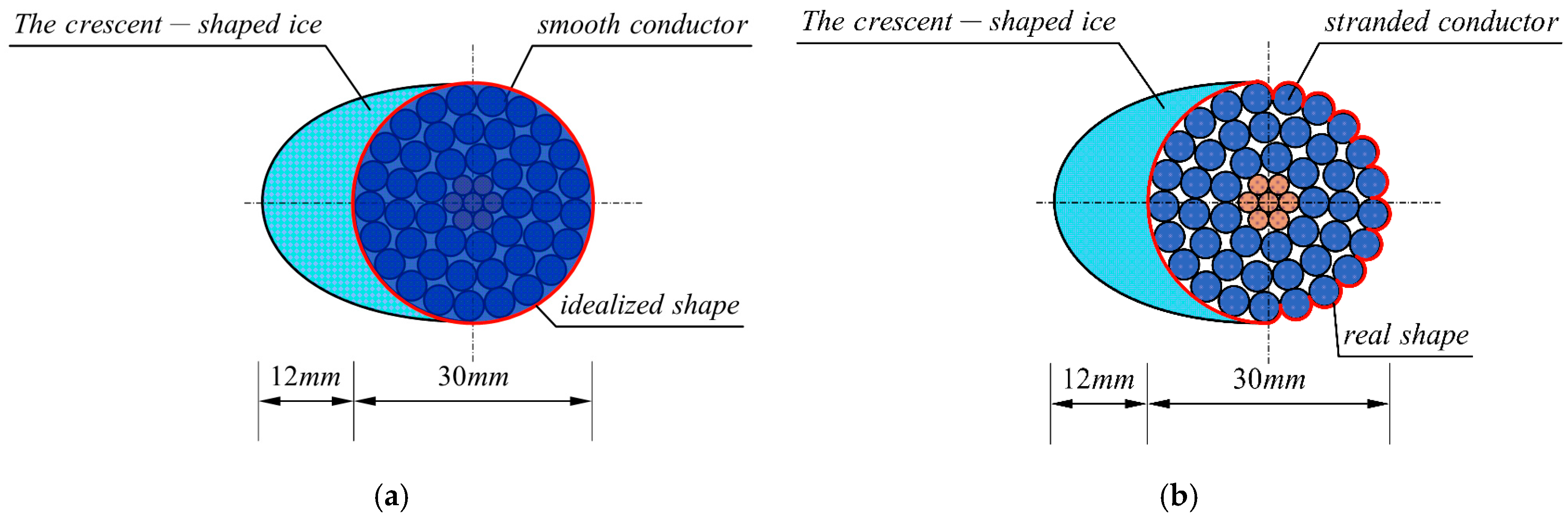
Numerical simulations often focus on idealized, smooth, and circular conductors. The influence of stranded geometry is frequently overlooked.
Figure 2 shows the schematic models used in this study. Wind tunnel tests were performed to obtain the aerodynamic parameters of the crescent-shaped iced conductor. Separate models were developed for the stranded and smooth sub-conductors.
2.2. Wind Tunnel Test
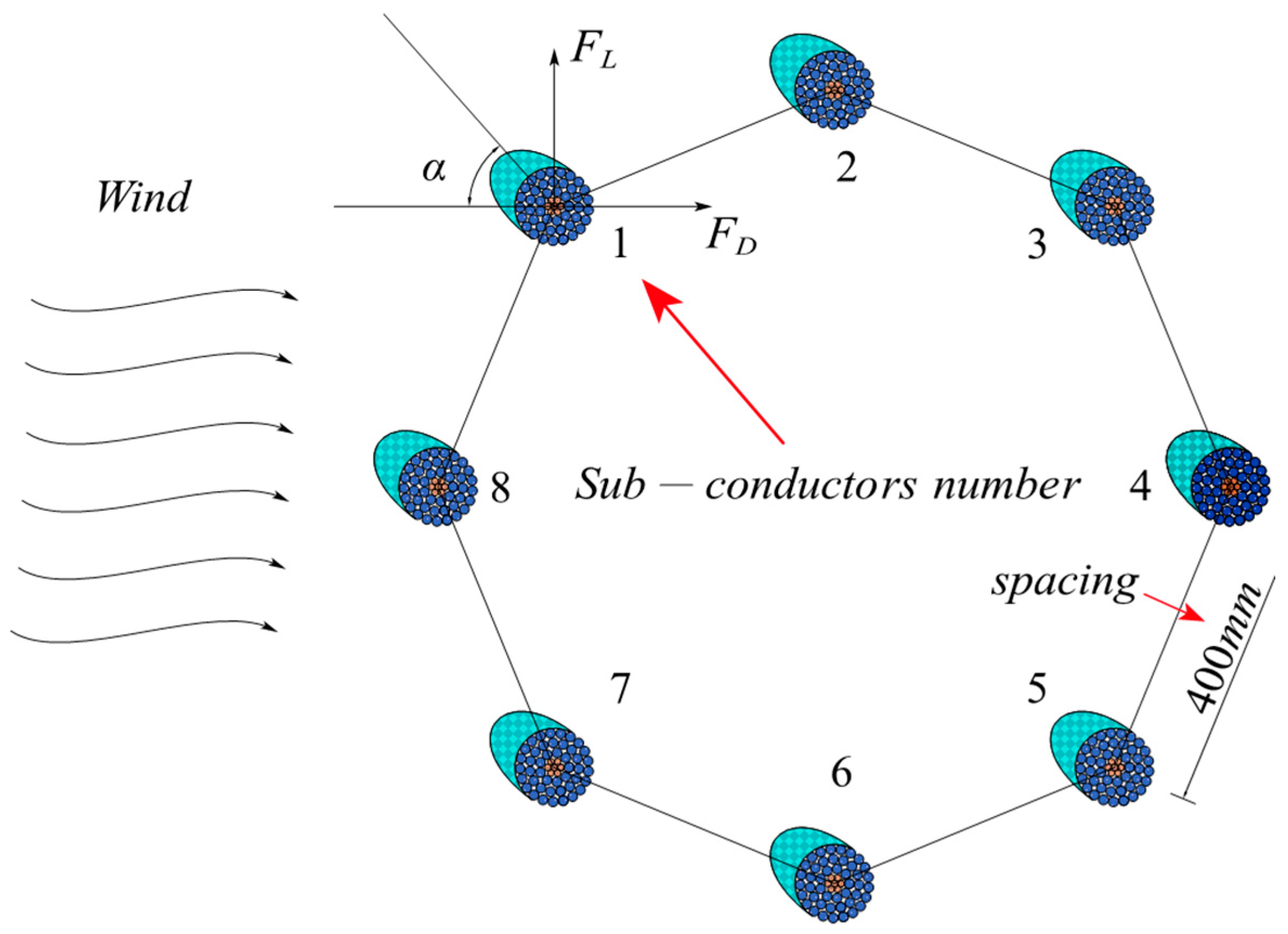
A wind angle of attack of 0° is defined when the incoming flow is parallel to the horizontal direction. A wind angle of 45° is set by rotating the incoming flow 45° clockwise. As shown in
Figure 3, lift is measured perpendicular to the inflow direction, while drag is measured parallel to and opposing the inflow.
A DC low-speed wind tunnel was used for the tests. The test section measured 2.8 m in length, 1.4 m in width, and 1.4 m in height. The central cross-sectional area was 1.92 m
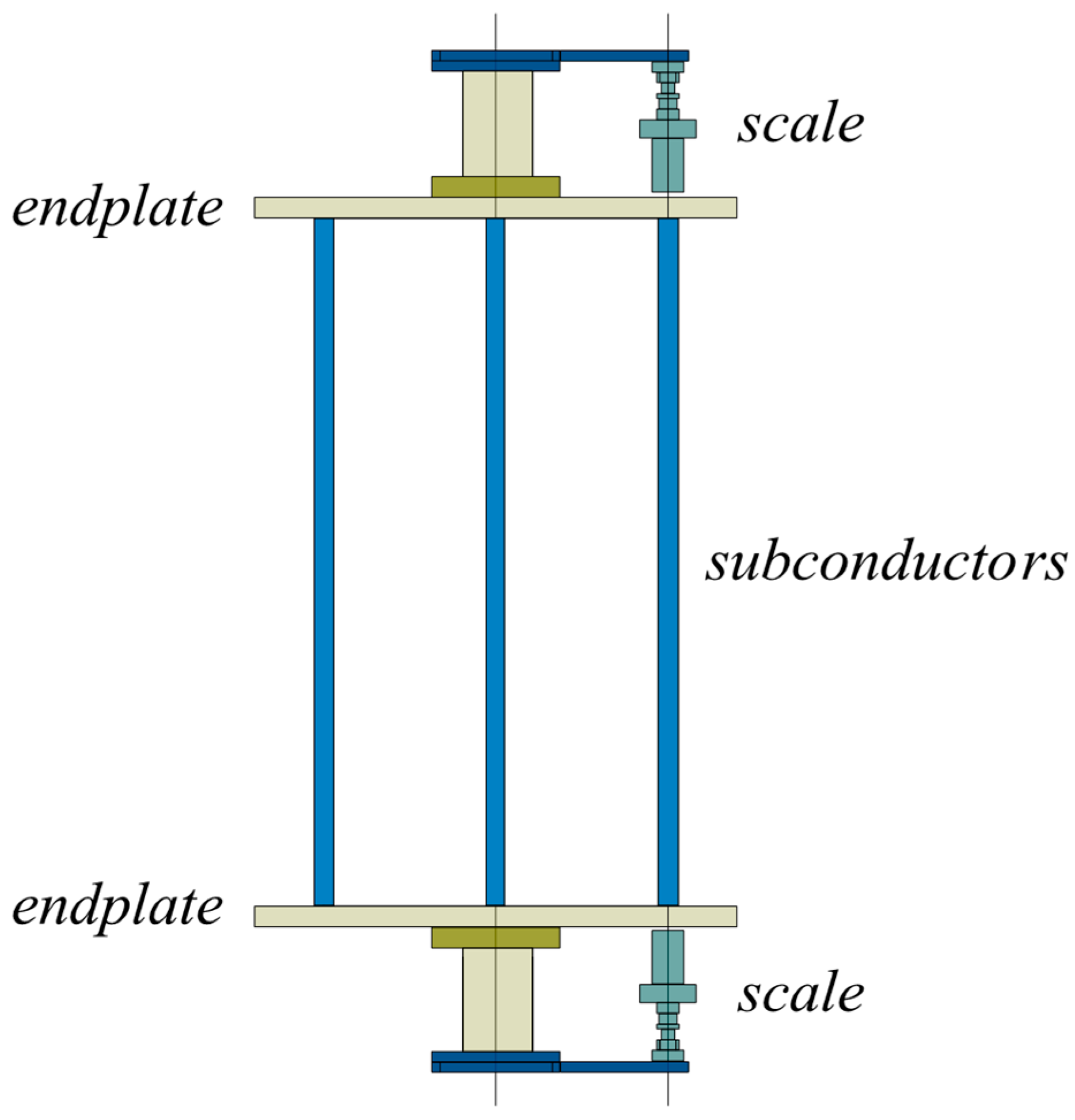
2. The inlet and outlet cut-off angles were 0.22 m and 0.18 m, respectively. The wind tunnel could operate at stabilized wind speeds from 0 m/s to 60 m/s. Force coefficients of the test conductor were measured using a two-point support method, as shown in
Figure 4. A DXTP scale set was used, and its main performance indicators are listed in
Table 2. The wind tunnel measurement and control system included three subsystems: a power system, a model attitude angle control system, and a data acquisition and processing system. The network control managed the attitude angle and power systems. The data acquisition system, based on NI-PXI architecture, used a hybrid SCXI/PXI chassis with 16 static/dynamic channels, 16-bit A/D resolution, and 0.05% static acquisition accuracy.
This test primarily examines the oscillation and aerodynamic properties of the iced conductor model under different working conditions [
19]. To optimize measurement accuracy and efficiency, a test condition was set at every 10° interval, resulting in a total of 19 test cases between 0° and 180°.
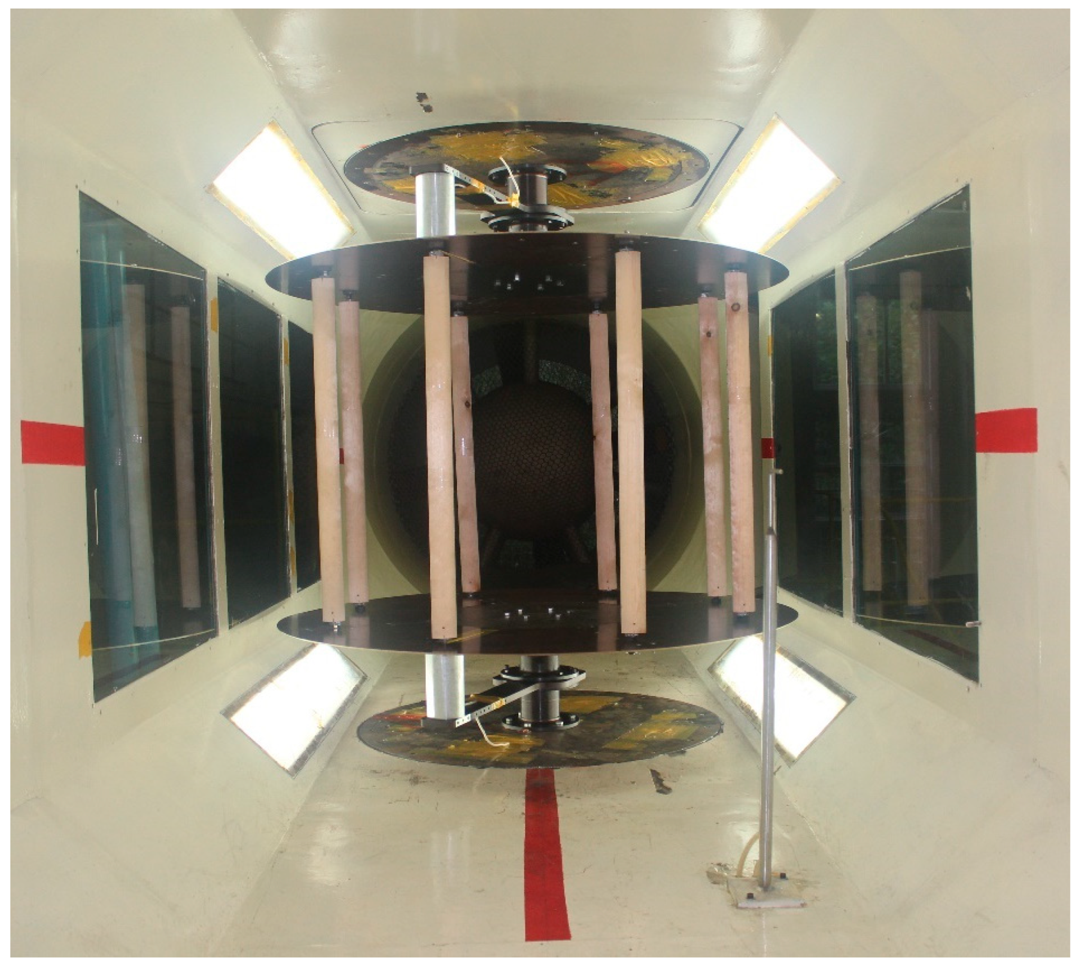
For the static force measurements, the iced eight-bundled conductor model was positioned vertically at the center of the circular end plate. Rigid supports connected the end plate to the wind tunnel’s upper and lower turntables. Inside the wind tunnel, the DXTP scale was attached to the upper and lower connections of the sub-conductor model and secured with a connecting plate. A windshield was installed on the scale. During testing, the upper and lower turntables were rotated synchronously to adjust the model’s orientation and angle of attack. Aerodynamic parameters of each sub-conductor were recorded. Grids were placed in front of the test section to generate turbulence. The wind tunnel test layout is shown in
Figure 5.
2.3. Governing Equations and Numerical Methods
The flow field has a flow velocity of 10 m/s, which is a low-velocity turbulent field and can be regarded as an incompressible flow [
20]. The Navier–Stokes equations for two-dimensional incompressible viscous flow are applied as the governing equations for this fluid domain.
Momentum equation:
where
and
represent the velocity components in the
and
directions, respectively.
represents time,
represents the fluid density, and
represents the pressure.
represents the dynamic viscosity of the fluid.
represents the volume force in the x-direction;
represents the volume force in the y-direction.
The SST
k-
ω turbulence model combines the Standard
k-
ω model for the near-wall region and the Standard
k-
ε model for the far-field region, making it well-suited for simulating both near-wall and far-field aerodynamic characteristics of the conductor. Its transport equations are as follows:
where
represents the turbulent kinetic energy;
represents the turbulent dissipation;
,
represents the mean turbulent velocity;
,
represents the coordinate component;
,
represents the turbulence generation terms;
,
represents the effective diffusion coefficients;
,
represents the dissipation terms; and
represents the cross-diffusion term. The role of
is to harmonize the Standard k-ε turbulence model with the Standard
k-
ω turbulence model junction region.
The aerodynamic properties of crescent-shaped iced eight-bundled conductors are primarily characterized by drag and lift forces. This study focuses on two force coefficients: the drag coefficient (
CD) and the lift coefficient (
CL), which are defined as follows:
where
FD represents the drag force acting on the iced conductor, while
FL denotes the lift force.
ρ is the density of the ambient air, given as 1.225 kg/m
3.
U is the mean incoming wind speed, set at 10 m/s.
B refers to the characteristic length of the cross-section of the crescent-shaped iced eight-bundled conductor model.
L is the model length, specified as 1 m.
The Reynolds number (
) is a dimensionless parameter that characterizes the state of fluid flow and is defined as follows:
The Reynolds numbers for all analyzed cases falls within the subcritical range, varying from 2.8 × 10
4 to 3.0 × 10
4.
2.4. Computational Domain and Boundary Conditions
CFD numerical simulation software(ANSYS Fluent 2023 R1) was used to simulate the crescent-shaped iced eight-bundled conductors with the coupled algorithm. The inlet was set as a velocity inlet, the outlet as a pressure outlet, and the upper and lower walls as symmetric boundaries. All other parameters were kept consistent with the wind tunnel test.
All numerical simulations were conducted using ANSYS Fluent 2023 R1. Geometric modeling and mesh generation were performed in ANSYS ICEM CFD. The pressure-based explicit transient solver was selected for all cases. The SST k-ω turbulence model was applied to accurately capture both near-wall and free-stream flow features. Pressure–velocity coupling was achieved using the coupled scheme. For spatial discretization, a second-order upwind scheme was used for momentum and turbulence equations. Second-order accuracy was adopted for time discretization. Residuals for all equations were required to drop below 1 × 10⁻⁶ for convergence.
The computational domain was defined as a rectangular box. The fluid domain diagram is shown in
Figure 6. The velocity inlet boundary was positioned 16D upstream of the conductor, the pressure outlet was set 33D downstream, and the upper and lower boundaries were placed 10D above and below the conductor axis, respectively, where D is the characteristic diameter of the conductor. The inlet boundary condition was a uniform velocity profile matching experimental wind speed. The outlet was set as a pressure outlet with zero-gauge pressure. The upper and lower boundaries were assigned as symmetry planes. The conductor surface was treated as a stationary no-slip wall. All other parameters and physical properties were kept consistent with the wind tunnel experiment.
2.5. Mesh Dependence Test and Validation
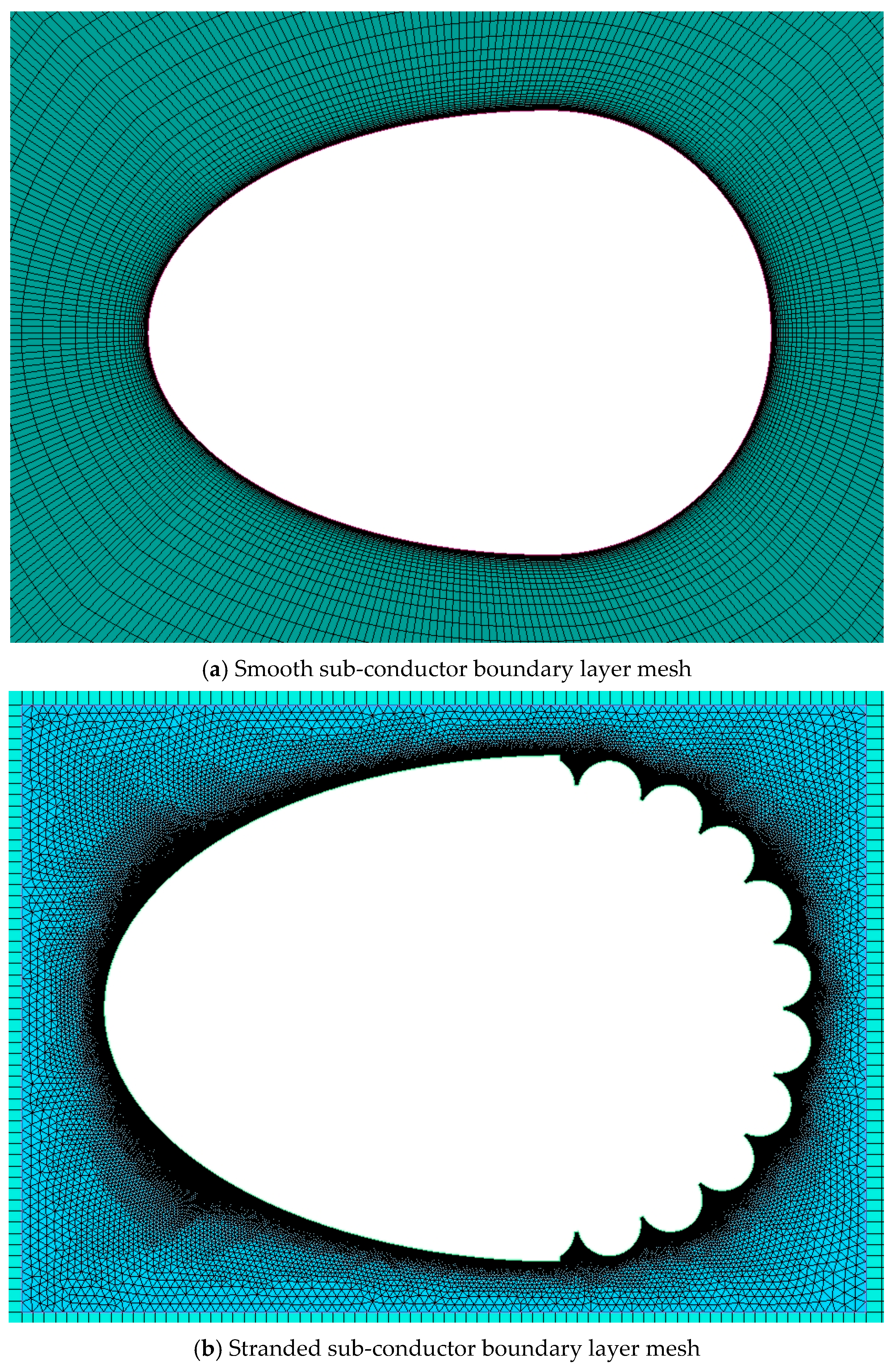
This CFD numerical simulation software employs the finite volume method to discretize the fluid domain using meshes. For smooth conductors, fully structured meshes are applied, whereas for stranded conductors, unstructured meshes are required in the region near the conductor due to its complex geometry [
21].
The
y+ value is a critical parameter for assessing mesh resolution near the wall. It represents the dimensionless height of the first wall-adjacent mesh cell and is defined as follows:
where
denotes the center height of the first-layer mesh cell adjacent to the wire, and
represents the wall friction velocity. In this study, the
value of the boundary layer mesh is maintained below 1, confirming that the meshing strategy meets the requirements for the numerical simulation. The boundary layer mesh is illustrated in
Figure 7.
The Strouhal number is a dimensionless number that describes the frequency characteristics in an oscillating fluid, and mesh dependence can be verified using it and other aerodynamic parameters. It is defined as follows:
where
represents the vortex frequency.
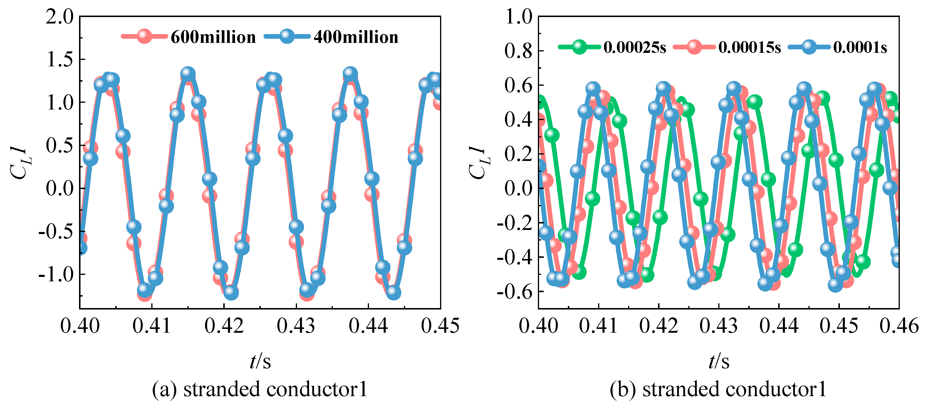
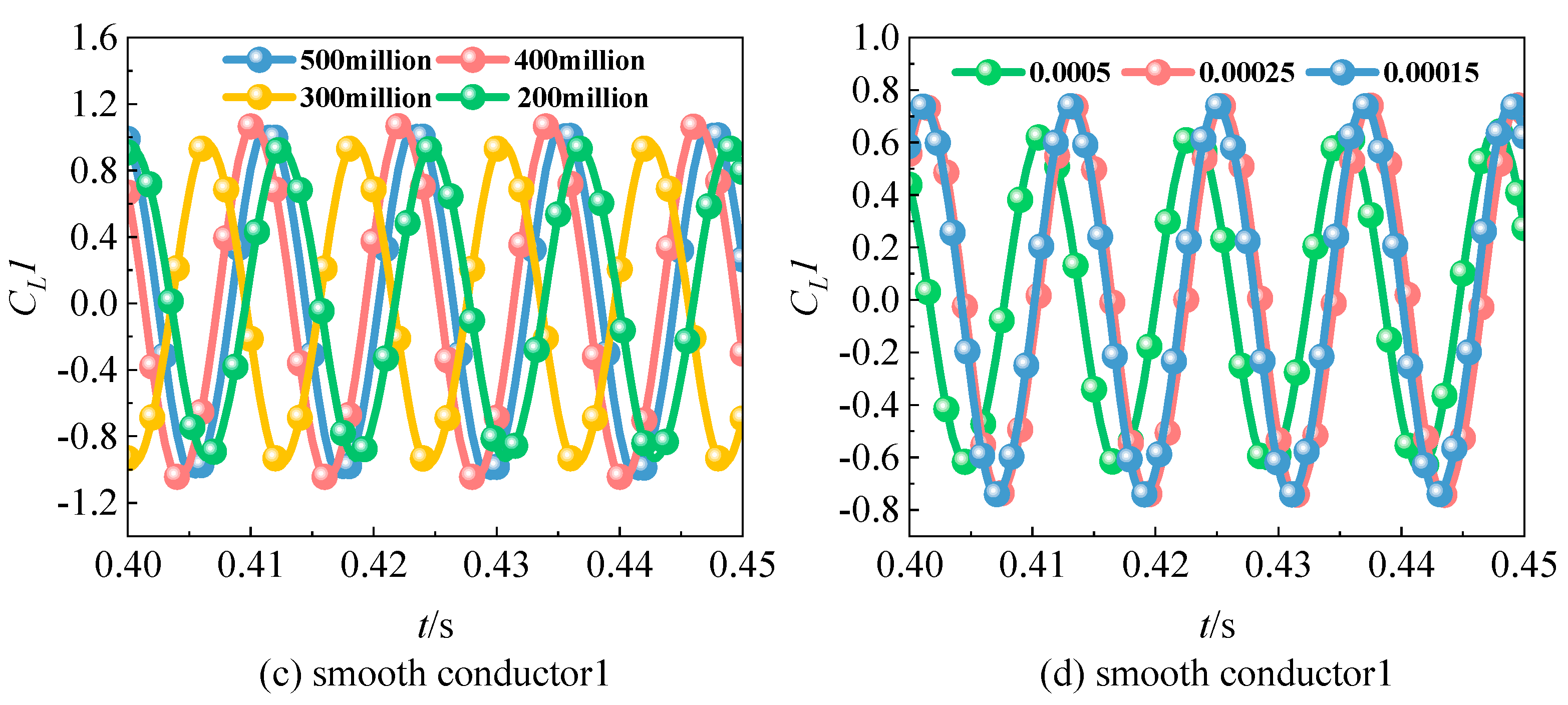
To ensure numerical accuracy, mesh independence and time-step sensitivity validations were performed on the computational mesh before calculations. The validation used the average drag coefficient, maximum lift coefficient, and Strouhal number. Their values are shown in
Table 3.
For smooth conductors, mesh dependence was studied using meshes ranging from 2 million to 5 million elements. Errors were found to decrease significantly at a mesh density of 4 million elements. For stranded conductors, the analysis was started with 4 million elements, which produced results consistent with those for smooth conductors. Therefore, a mesh density of 4 million elements was adopted for all simulations.
Time-step sensitivity validation was performed in a similar manner. The optimal time step differed between conductor types: 0.00025 s was used for smooth conductors, while 0.00015 s was required for stranded conductors. The suitability of the selected mesh density and time-step size is shown in
Figure 8.
3. Results and Discussion
3.1. Analysis of Aerodynamic Characteristics
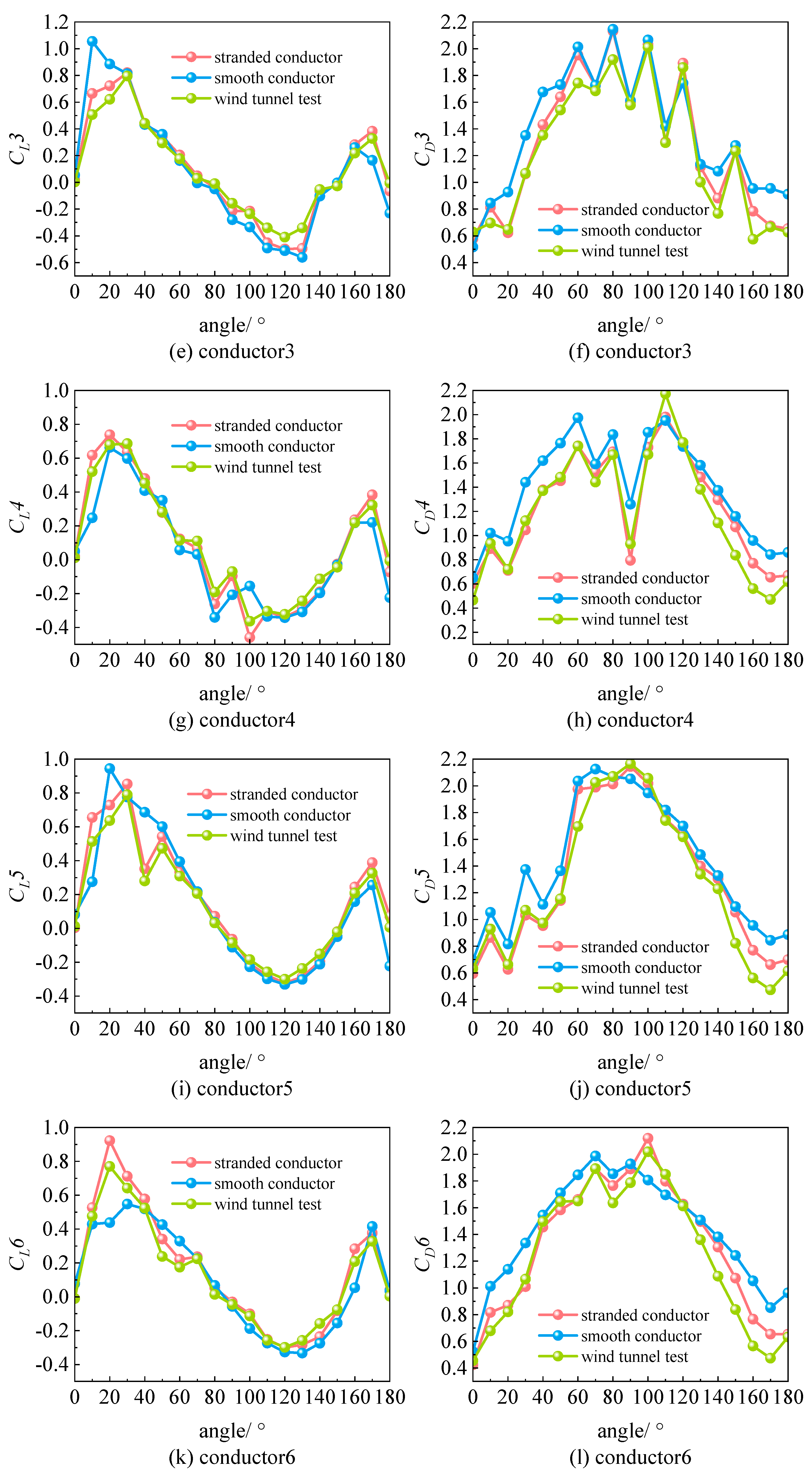
As shown in
Figure 9, numerical simulation results for crescent-shaped iced eight-bundled conductors 1 to 8 are presented together with lift and drag coefficients from wind tunnel tests. The stranded conductor simulations show much closer agreement with experimental results, both in trend and overall behavior. In contrast, simulations for smooth conductors display larger discrepancies, especially in the lift coefficient near a 20° wind angle of attack. Drag coefficient errors for smooth conductors are also much higher, particularly near 20° and 170°. These differences highlight the significant impact of conductor geometry on aerodynamic simulation accuracy.
Analysis of the lift coefficient curves shows that both numerical simulations and wind tunnel tests exhibit a sharp increase in lift near 20° and 170° angles of attack, forming a distinct “peak.” To investigate this, simulations for both stranded and smooth conductors were performed, and the corresponding pressure contour plots were analyzed, as shown in
Figure 10. For sub-conductor 8 at a 20° wind angle, a significant negative pressure area appears on the upper left side, while high pressure develops on the lower left (windward) side. A smaller negative pressure region is observed on the lower right. This pressure distribution generates a substantial lift. At a 170° wind angle, the lift increase follows a different pattern. Both the upper and lower sides are in negative pressure regions, but the upper zone has higher negative pressure values, creating a smaller “lift peak” at this angle.
Figure 10 shows two vortices, one large and one small, forming on the right side, with the suction effect further influencing the lift and contributing to the peak. Flow patterns differ significantly between stranded and smooth conductors, causing greater pressure fluctuations in the simulations. At 20°, the negative pressure region on the stranded conductor is larger, with more pronounced pressure changes. The stranded geometry causes two vortices of different sizes and shapes to form on the right. At 170°, the stranded conductor does not form a small vortex on the upper right, unlike the smooth conductor. Instead, the stranded geometry blocks its formation, leading to a larger and denser vortex closer to the conductor.
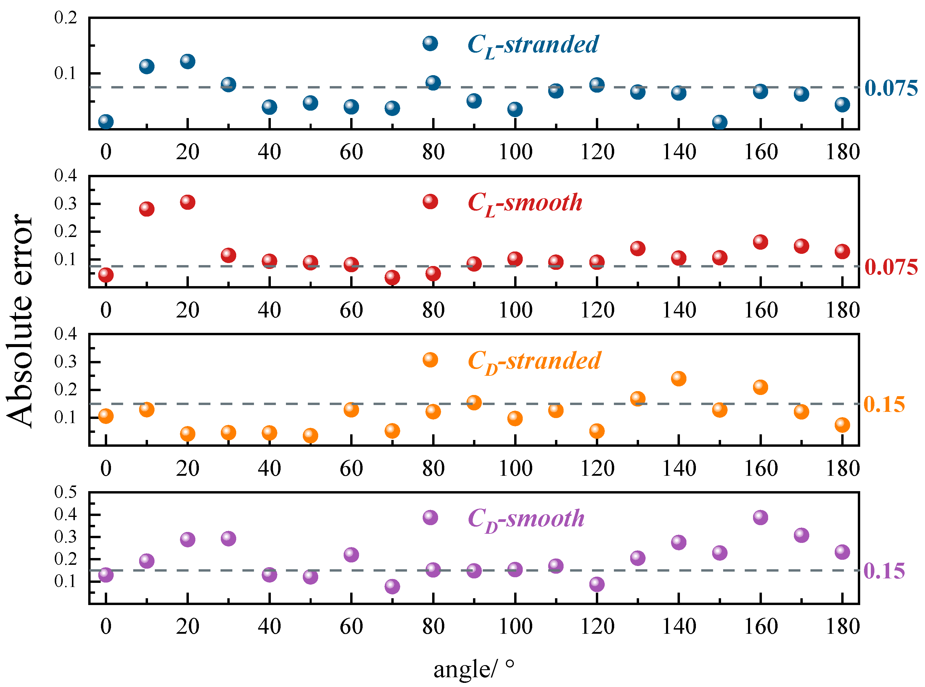
In summary, a direct comparison of experimental and simulated data across all eight conductors reveals clear differences in accuracy between smooth and stranded models.
Figure 11 shows the absolute error values of the lift coefficient and drag coefficient. For the lift coefficient, the average error for stranded conductors remains around 0.075, with a maximum of 0.13, while the smooth model exhibits larger discrepancies, with typical errors near 0.1 and a maximum reaching 0.3. For the drag coefficient, the average error for stranded conductors stays within 0.15 and peaks at about 0.24, compared to average errors of approximately 0.2 and a maximum of 0.4 for smooth conductors. Incorporating the stranded geometry results in a 45–50% reduction in mean errors for both lift and drag coefficients. These results confirm that high-fidelity modeling of the stranded structure significantly improves the agreement between simulation and experiment for all sub-conductors, providing a more reliable framework for aerodynamic prediction and engineering application.
3.2. Analysis of Wake Effects
Analysis of the drag coefficient curves indicates that the windward profile of the conductors resembles a “bullet” at wind angles of 0° and 180°. As shown in
Figure 12, the windward area is minimized at these angles, with conductors 1, 2, 7, and 8 facing the wind. The leeward sub-conductors experience only a small low-speed region in the wake flow. As a result, the drag coefficients for these sub-conductors remain low. At a wind angle of 90°, the windward profile changes to a “shield,” producing the largest windward area. At this angle, conductors 5, 6, 7, and 8 face the wind. A large low-speed region forms in the wake of the leeward sub-conductors, where velocity drops to 1–3 m/s. The drag coefficients for the windward sub-conductors reach maximum values due to blockage by the iced conductor. In contrast, the leeward conductors experience a sharp drop in wind speed and are shadowed by the windward conductors, leading to a sudden decrease in their drag coefficients. This sudden drop is not observed at 80° and 100°, owing to differences in conductor arrangement and windward profile at those angles.
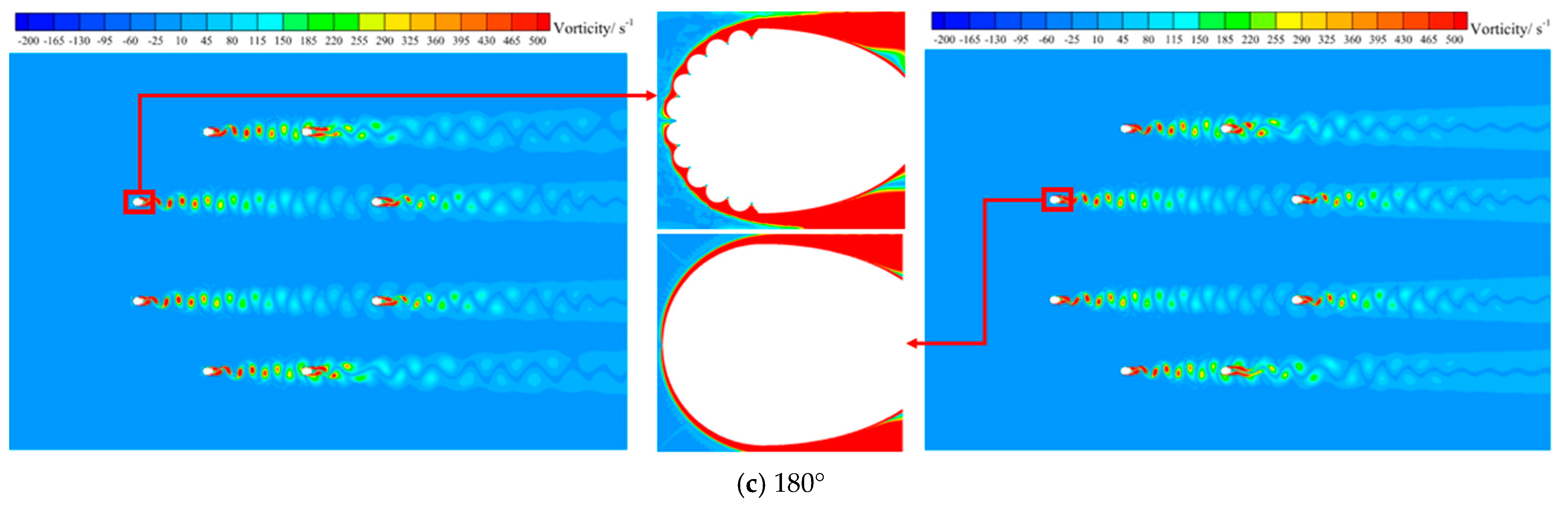
Figure 13 shows the vortex contours for the crescent-shaped iced eight-bundled conductors at wind angles of 0°, 90°, and 180°. The distance between sub-conductors 1, 4, 5, and 8 is about 965 mm, while that between sub-conductors 2, 3, 6, and 7 is 400 mm.
At a 0° wind angle, the sub-conductors align with the streamlines, resulting in a reduced wake effect. The vortex pattern appears as two strips partially wrapping around the conductor. This effect is more pronounced for sub-conductors that are closer together, such as 2 and 3 or 6 and 7, than for those farther apart, like 1 and 4 or 5 and 8. At a 90° wind angle, the wake effect increases significantly. Vortex density in the near-wake region decreases, while a large accumulation of vortices form on the leeward side. The wake exhibits a “thin upper strip and thicker lower strip” structure. At 180°, the proximity of sub-conductors 2 and 3, as well as 6 and 7, strongly affects the size and strength of generated vortices. The wake region displays “darting strip” vortices, while the windward side forms half-wrapped strips. At all three wind angles, sub-conductors at the top of the domain are less affected by wakes than those at the bottom, and the central sub-conductors are minimally influenced.
The stranded geometry also impacts wake development. At 0°, neglecting the suction effects of vortices formed in the gaps between strands can lead to significant simulation deviations. At 90°, wake effects in the leeward region are more pronounced, while the vortex around smooth sub-conductors 3 and 6 becomes a fluttering strip, deviating from the expected pattern. At 180°, the stranded geometry further alters vortex distribution, influencing lift and drag forces and reducing simulation errors.
3.3. Analysis of the Vertical Oscillation Mechanism
The vertical oscillation mechanism proposed by Den Hartog, based on the combined effects of drag and lift, is widely accepted by researchers. When the negative slope of the lift coefficient curve exceeds the drag coefficient, vertical oscillations of the conductors may be induced [
22]. The formula for this mechanism is defined as follows:
where
represents the Den Hartog coefficient;
represents the wind angle of attack.
The Den Hartog coefficient is crucial for predicting conductor oscillation [
23]. Because this coefficient depends on the slope of the lift coefficient curve, it is important that the simulated lift coefficient matches both the values and trends observed in wind tunnel tests. Only then can the accuracy of vertical oscillation predictions be ensured.
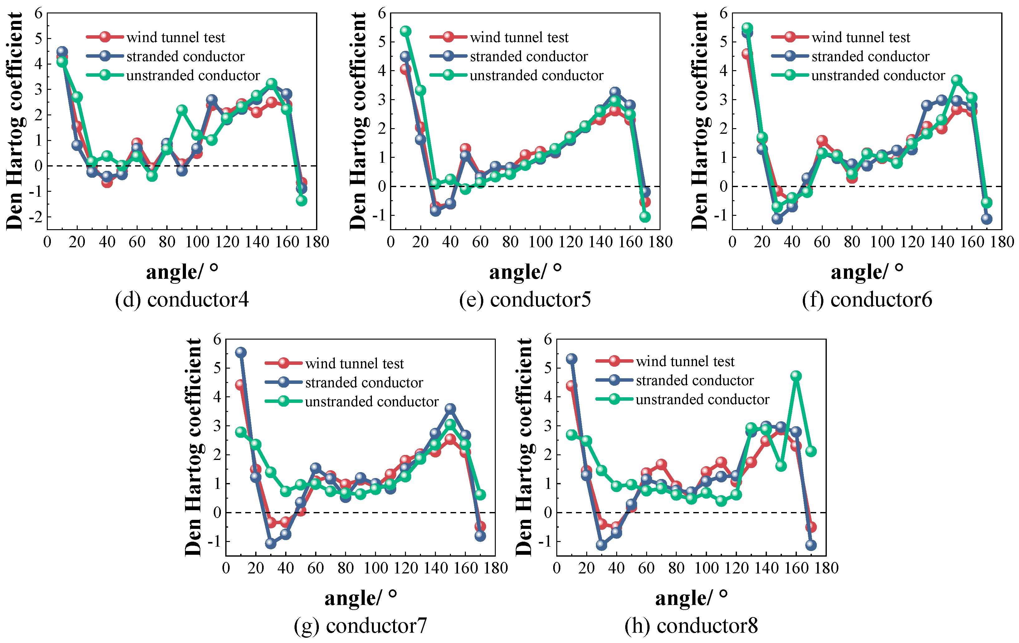
As shown in
Figure 14, the Den Hartog coefficient from wind tunnel tests becomes negative at wind angles where the lift coefficient shows a “peak phenomenon.” At these angles, conductors are highly susceptible to vertical oscillation. For smooth conductors, the simulation trend for the lift coefficient deviates significantly from the wind tunnel results. In total, 20 simulated points do not match the test, resulting in an error rate of 15.6%. In contrast, the simulation for stranded conductors is much more accurate, with only five points deviating, giving an error rate of just 3.9%. These results highlight the importance of including stranded geometry in simulations of iced conductors. Simulations that account for stranded geometry show much higher accuracy.
4. Conclusions
The aerodynamic characteristics and wake effects of iced eight-bundled stranded conductors were systematically investigated using wind tunnel experiments and numerical simulations. The results highlight the pivotal role of stranded geometry in high-fidelity aerodynamic predictions and identify critical wind angles that trigger conductor instability. The main conclusions are as follows:
(1) Explicit modeling of the stranded surface significantly enhances simulation accuracy. Incorporating stranded geometry, compared to smooth models, reduces average errors in lift and drag coefficients by 45–50%. The error in predicting the Den Hartog coefficient decreases from 15.6% to 3.9%. Improved geometric fidelity directly leads to better oscillation predictions.
(2) Distinct peaks in the lift coefficient and abrupt pressure transitions occur at wind angles of 20° and 170°. These features result from asymmetric vortex shedding and localized negative pressure zones. They correspond to steep gradients in the Den Hartog coefficient, marking these angles as critical for vertical oscillation onset.
(3) Wake intensity is influenced by both the windward area and the spatial arrangement of sub-conductors. At a 90° wind angle, maximal windward exposure amplifies turbulence and reduces leeward velocity to 1–3 m/s. Lower sub-conductors experience stronger wake interference, while central conductors show minimal variation. This highlights the need for position-specific design strategies.
(4) The validated numerical framework provides a cost-effective tool for predicting icing-induced galloping in ultra-high-voltage lines. Simulation practices should prioritize stranded geometry and enhance structural damping at critical wind angles, such as 20° and 170°, to improve operational stability.
By integrating high-fidelity geometric modeling into numerical simulations, this study advances the prediction of icing-induced galloping in multi-bundled conductors and provides a solid foundation for improving transmission line stability in cold climates.
Author Contributions
Conceptualization, B.Z. and M.C.; methodology, B.Z.; software, B.Z.; validation, J.S.; formal analysis, M.H.; investigation, M.H.; resources, M.C.; data curation, M.H.; writing—original draft preparation, B.Z.; writing—review and editing, M.C.; visualization, J.S.; supervision, M.C.; project administration, B.Z.; funding acquisition, M.C. All authors have read and agreed to the published version of the manuscript.
Funding
The work described in this paper is supported by the China Postdoctoral Science Foundation (Funding number: 2021M702371).
Data Availability Statement
Data available on request from the authors.
Conflicts of Interest
The authors declare no conflicts of interest.
References
- Matsumiya, H.; Yukino, T.; Shimizu, M.; Nishihara, T. Field observation of galloping on four-bundled conductors and verification of countermeasure effect of loose spacers. J. Wind Eng. Ind. Aerodyn. 2022, 220, 104859. [Google Scholar] [CrossRef]
- Liu, C.; Zhang, Y.; Ma, W.; Song, Y. Numerical Simulation and Analysis of the Influencing Factors of Ice Formation on Electrified Railway Contact Lines. Infrastructures 2025, 10, 121. [Google Scholar] [CrossRef]
- Zhang, L.; Zhou, X.; Ruan, J.; Feng, Z.; Shen, Y.; Yao, Y. Failure Analysis and Safety De-Icing Strategy of Local Transmission Tower-Line Structure System Based on Orthogonal Method in Power System. Processes 2025, 13, 1782. [Google Scholar] [CrossRef]
- Taruishi, S.; Matsumiya, H. Investigation of effect of galloping countermeasures for four-bundled conductors through field observations. Cold Reg. Sci. Technol. 2023, 214, 103962. [Google Scholar] [CrossRef]
- Zhao, M.; Li, M.; Li, S.; Wan, Y.; Hai, Y.; Li, C. Galloping Performance of Transmission Line System Aeroelastic Model with Rime Through Wind-Tunnel Tests. Energies 2025, 18, 1203. [Google Scholar] [CrossRef]
- Veerakumar, R.; Tian, L.; Hu, H.; Liu, Y.; Hu, H. An experimental study of dynamic icing process on an Aluminum-Conductor-Steel-Reinforced power cable with twisted outer strands. Exp. Therm. Fluid Sci. 2023, 142, 110823. [Google Scholar] [CrossRef]
- Zhang, Z.; Han, Y.; Yu, J.; Hu, P.; Cai, C.S. Anti-galloping analysis of iced quad bundle conductor based on compound damping cables. Eng. Struct. 2024, 306, 117831. [Google Scholar] [CrossRef]
- Wu, Y.; Chen, X. Prediction and characterization of three-dimensional multi-mode coupled galloping of multi-span ice-accreted transmission conductors. J. Wind Eng. Ind. Aerodyn. 2023, 241, 105516. [Google Scholar] [CrossRef]
- Lou, W.J.; Zhang, Y.L.; Gu, Y.; Luo, G.; Bai, H.; Huang, M.F.; Virk, M.S.; Bian, R. An improved rigid rod method for wind-induced swing response prediction of heavily iced transmission lines. J. Wind Eng. Ind. Aerodyn. 2023, 235, 105358. [Google Scholar] [CrossRef]
- Zhitao, Y.; Yi, Y.; Xiaogang, Y.; Wensheng, L.; Cheng, H.; Chun, N.X.; Jun, L. Numerical Simulation of Fluid-Structure Interaction of D-shape Iced Conductor. Eur. J. Comput. Mech. 2019, 28, 147–170. [Google Scholar] [CrossRef]
- Wan, Z.; Zhang, D.; Li, Z.; Mo, S.; Zhang, Y. A wind tunnel study on the aerodynamic characteristics of ice-accreted twin bundled conductors. Int. J. Struct. Stab. Dyn. 2022, 22, 2250038. [Google Scholar] [CrossRef]
- Lou, W.; Chen, S.; Wen, Z.; Wang, L.; Wu, D. Effects of ice surface and ice shape on aerodynamic characteristics of crescent-shaped iced conductors. J. Aerosp. Eng. 2021, 34, 04021008. [Google Scholar] [CrossRef]
- Liao, S.; Zhang, Y.; Chen, X.; Cao, P. Research on Aerodynamic Characteristics of Crescent Iced Conductor Based on SA Finite Element Turbulence Model. Energies 2022, 15, 7753. [Google Scholar] [CrossRef]
- Li, J.X.; Sun, J.; Ma, Y.; Wang, S.H.; Fu, X. Study on the aerodynamic characteristics and galloping instability of conductors covered with sector-shaped ice by a wind tunnel test. Int. J. Struct. Stab. Dyn. 2020, 20, 2040016. [Google Scholar] [CrossRef]
- Chen, Z.; Cai, W.; Su, J.; Nan, B.; Zeng, C.; Su, N. Aerodynamic force and aeroelastic response characteristics analyses for the galloping of ice-covered four-split transmission lines in oblique flows. Sustainability 2022, 14, 16650. [Google Scholar] [CrossRef]
- Qing, H.; Jian, Z.; Mengyan, D.; Dongmei, D.; Makkonen, L.; Tiihonen, M. Rime icing on bundled conductors. Cold Reg. Sci. Technol. 2019, 158, 230–236. [Google Scholar] [CrossRef]
- Cai, M.; Yang, X.; Huang, H.; Zhou, L. Investigation on galloping of D-shape iced 6-bundle conductors in transmission tower line. KSCE J. Civ. Eng. 2020, 24, 1799–1809. [Google Scholar] [CrossRef]
- Zhou, L.; Yan, B.; Zhang, L.; Zhou, S. Study on galloping behavior of iced eight bundle conductor transmission lines. J. Sound Vib. 2016, 362, 85–110. [Google Scholar] [CrossRef]
- Lu, J.; Wang, Q.; Wang, L.; Mei, H.; Yang, L.; Xu, X.; Li, L. Study on wind tunnel test and galloping of iced quad bundle conductor. Cold Reg. Sci. Technol. 2019, 160, 273–287. [Google Scholar] [CrossRef]
- Lou, W.; Huang, C.; Huang, M.; Yu, J. An aerodynamic anti-galloping technique of iced 8-bundled conductors in ultra-high-voltage transmission lines. J. Wind Eng. Ind. Aerodyn. 2019, 193, 103972. [Google Scholar] [CrossRef]
- Matsumiya, H.; Yagi, T.; Macdonald, J.H. Effects of aerodynamic coupling and non-linear behaviour on galloping of ice-accreted conductors. J. Fluids Struct. 2021, 106, 103366. [Google Scholar] [CrossRef]
- Den Hartog, J.P. Transmission line vibration due to sleet. Trans. Am. Inst. Electr. Eng. 1932, 51, 1074–1076. [Google Scholar] [CrossRef]
- Chao, Z.; Jiaqi, Y. Glaze icing process of moveable overhead conductor and its aerodynamic characteristics with numerical method. Int. J. Heat Mass Transf. 2021, 176, 121436. [Google Scholar] [CrossRef]
Figure 1.
LGJ-500/35 conductor and light wood.
Figure 1.
LGJ-500/35 conductor and light wood.
Figure 2.
(a) Schematic diagram of the smooth sub-conductor model and (b) schematic diagram of the stranded sub-conductor model.
Figure 2.
(a) Schematic diagram of the smooth sub-conductor model and (b) schematic diagram of the stranded sub-conductor model.
Figure 3.
Define the wind angle of attack and sub-conductor number.
Figure 3.
Define the wind angle of attack and sub-conductor number.
Figure 4.
Wind tunnel test program layout.
Figure 4.
Wind tunnel test program layout.
Figure 5.
Wind tunnel test layout.
Figure 5.
Wind tunnel test layout.
Figure 6.
The fluid domain diagram.
Figure 6.
The fluid domain diagram.
Figure 7.
Smooth sub-conductor boundary layer mesh (a) and stranded sub-conductor boundary layer mesh (b).
Figure 7.
Smooth sub-conductor boundary layer mesh (a) and stranded sub-conductor boundary layer mesh (b).
Figure 8.
(a) Stranded conductor 1 mesh dependence, (b) stranded conductor 1 time-step dependence, (c) smooth conductor 1 mesh dependence, and (d) smooth conductor 1 time-step dependence.
Figure 8.
(a) Stranded conductor 1 mesh dependence, (b) stranded conductor 1 time-step dependence, (c) smooth conductor 1 mesh dependence, and (d) smooth conductor 1 time-step dependence.
Figure 9.
Sub-conductors lift coefficient and drag coefficient curves (a–p).
Figure 9.
Sub-conductors lift coefficient and drag coefficient curves (a–p).
Figure 10.
Pressure contours of stranded and smooth conductor 8 at 20° and 170° wind angles of attack.
Figure 10.
Pressure contours of stranded and smooth conductor 8 at 20° and 170° wind angles of attack.
Figure 11.
Absolute error of lift coefficient and drag coefficient.
Figure 11.
Absolute error of lift coefficient and drag coefficient.
Figure 12.
Velocity contours for wind attack angles of 0° (a), 90° (b), and 180° (c).
Figure 12.
Velocity contours for wind attack angles of 0° (a), 90° (b), and 180° (c).
Figure 13.
The vortex contours for conductors at 0° (a), 90° (b), and 180° (c) wind angles of attack.
Figure 13.
The vortex contours for conductors at 0° (a), 90° (b), and 180° (c) wind angles of attack.
Figure 14.
Den Hartog coefficients for sub-conductors 1–8 (a–h).
Figure 14.
Den Hartog coefficients for sub-conductors 1–8 (a–h).
Table 1.
Parameters of the sub-conductors (diameter, mm).
Table 1.
Parameters of the sub-conductors (diameter, mm).
| Sub-Conductor Model | Aluminum Strands (Number/Diameter, mm) | Steel Strands (Number/Diameter, mm) | Number of Outermost Strands (Number/Diameter, mm) | Outer Diameter (mm) |
|---|
| LGJ-500/35 | 45/3.75 | 7/2.50 | 21/3.75 | 30 |
Table 2.
The main performance index table of the scale.
Table 2.
The main performance index table of the scale.
| Component | Y | X | Mz | Z | My | Mx |
|---|
| Design load (N, N·m) | 100 | / | 20 | 100 | 20 | 5 |
| Calibration Load (N, N·m) | 100 | / | 10 | 100 | 7.5 | 5 |
| Precision (%) | 0.05 | / | 0.05 | 0.05 | 0.05 | 0.05 |
| Accuracy (%) | 0.3 | / | 0.2 | 0.2 | 0.3 | 0.2 |
Table 3.
Comparison of force coefficients.
Table 3.
Comparison of force coefficients.
| Conductor Type | Number of Meshes (Million) | Time Step(s) | | | St |
|---|
| smooth | 2 | 0.001 | 0.51988 | 0.93319 | 0.2414 |
| smooth | 3 | 0.001 | 0.52674 | 0.96178 | 0.2495 |
| smooth | 4 | 0.001 | 0.74338 | 1.08411 | 0.2579 |
| smooth | 5 | 0.001 | 0.73187 | 1.07208 | 0.2597 |
| stranded | 4 | 0.001 | 0.66982 | 1.33686 | 0.2620 |
| stranded | 6 | 0.0005 | 0.65736 | 1.31899 | 0.2616 |
| smooth | 4 | 0.0005 | 0.45517 | 0.66659 | 0.2513 |
| smooth | 4 | 0.00025 | 0.51205 | 0.74309 | 0.2623 |
| smooth | 4 | 0.00015 | 0.501 | 0.74199 | 0.2649 |
| stranded | 4 | 0.00025 | 0.66115 | 0.55894 | 0.2584 |
| stranded | 4 | 0.00015 | 0.69132 | 0.60622 | 0.2617 |
| stranded | 4 | 0.0001 | 0.68517 | 0.59768 | 0.2639 |
| Disclaimer/Publisher’s Note: The statements, opinions and data contained in all publications are solely those of the individual author(s) and contributor(s) and not of MDPI and/or the editor(s). MDPI and/or the editor(s) disclaim responsibility for any injury to people or property resulting from any ideas, methods, instructions or products referred to in the content. |
© 2025 by the authors. Licensee MDPI, Basel, Switzerland. This article is an open access article distributed under the terms and conditions of the Creative Commons Attribution (CC BY) license (https://creativecommons.org/licenses/by/4.0/).


