Tailoring a Three-Layer Track Model to Delay Instability and Minimize Critical Velocity Effects at Very High Velocities

Abstract

The aim of this paper is to tailor the geometry and material parameters of a three-layer railway track model to achieve favorable properties for the circulation of high-speed trains at very high velocities. The three layers imply that the model should have three critical velocities for resonance. However, in many cases, some of these values are missing and must be replaced by pseudo-critical values. Since no resonance occurs at pseudo-critical velocities, even in the absence of damping, deflections never reach infinity. By using optimization techniques, it is possible to adjust the model’s parameters, so that the increase in vibrations remains minimal and does not pose a real danger. In this way, circulation velocities could be extended beyond the critical value, thereby increasing the network capacity and, consequently, improving the competitiveness of rail transport compared to other modes of transportation, thus contributing to decarbonization. The presented results are preliminary and require further analysis and validation. Several optimization techniques are implemented, leading to the establishment of designs that already have rather high pseudo-critical velocities. Further research will show how these theoretical findings can be utilized in practice.

1. Introduction

The railway enables the circulation of railway vehicles in a safe and comfortable manner. Prioritizing rail transport over road transport represents an effective approach to combating climate change and reducing the carbon footprint. In line with this, it is necessary to increase the capacity of the railway network, without compromising passenger safety and comfort. To achieve this, the adequate transfer of solicitations to the ground must be ensured. Given the high demands that rolling stock imposes on the railway, one of the most challenging problems is identifying the most suitable technical solutions that are capable of supporting an increase in traffic velocity under standardized conditions, without compromising vehicle ride quality.

For the above reasons, high-speed trains are increasingly essential in today’s world, due to their environmental, economic, and practical advantages. As a sustainable mode of transportation, they consume less energy and produce fewer emissions compared to cars and airplanes, particularly over medium distances. By efficiently connecting major cities and economic centers, high-speed railways foster regional development, facilitate business and tourism, and boost productivity through reduced travel times. It also helps alleviate congestion on roads and at airports, offering a reliable and comfortable alternative for travelers. Moreover, high-speed rail systems enhance passenger convenience, with smooth, spacious, and punctual services, often outperforming air travel when considering the overall journey time. Finally, investment in high-speed railways drives technological innovation, generates employment, and contributes to the modernization of national infrastructure.

The maximum attainable circulation velocity in railway systems is often constrained by the so-called critical velocity, which, in the context of a moving force, represents the lowest velocity at which waves can propagate through the supporting track structure. This velocity arises from the dynamic interplay between all the structural components and corresponds to a resonance condition. Experimental data indicate that this threshold has already been reached under real operating conditions [1].

To deepen our understanding of such dynamic behavior, further investigations are conducted within the well-established framework of moving-load problems, a subject that continues to attract significant interest in transportation engineering. To enhance computational tractability and facilitate optimization and sensitivity analyses, many studies adopt simplified models. These simplifications can pertain to either the structure, the vehicle, or both, depending on the specific aspect under study. In addition to exploring the effect of key parameters on the dynamic response, major areas of interest include resonance-related critical velocities and frequencies, system instability, and the interaction between moving neighboring inertial bodies.

Among the first studies to provide the necessary physical basis for resonance near the Rayleigh wave velocity in regard to the ground or bending wave velocity of the track are [2,3]. These early works analyze how loads moving on an elastic beam or layer over an elastic half-space lead to resonance or pseudo-resonance at specific velocities. They provided fundamental insights into wave propagation and resonance phenomena in layered ground–structure systems and were instrumental in identifying the key mechanisms behind critical velocity effects. Analytical formulations are used to determine key wave velocities and describe how layering and stiffness contrast influence the equivalent dynamic stiffness and resonance conditions. In [4], semi-analytical models for wave propagation in a layered elastic or viscoelastic half-space under train loading are developed. The authors establish how train speeds approaching critical values lead to amplified ground vibrations. These works were fundamental in describing critical velocity phenomena and track–ground interactions, offering closed-form solutions for simplified models.

Further, in [5], the influence of nonlinear soil behavior and soil layering on the dynamic performance of high-speed railway track systems, particularly near critical velocities, is investigated. An equivalent linear model within the context of the 2.5D finite/infinite elements method is proposed and validated against experimental results. Additionally, these results are compared with those obtained using a linear elastic model, as commonly applied in the assessment of vibrations induced by traffic. The authors use a numerical model combining a train–track system with a multi-layered soil domain and show that nonlinearities in the subgrade can significantly affect resonance phenomena and vibration amplification. The paper also explores how certain design adjustments (e.g., modifying stiffness and damping) could mitigate these effects, making it one of the first studies to explicitly link track–soil dynamics to design strategies for improved performance at high velocities. These works inspired later multi-layer and numerical optimizations, such as the engineering applications described in [6], which exploit detailed 3D finite element models to simulate train–track–ground systems, including realistic rail, sleeper, ballast, and subgrade layers. They demonstrated how adjusting the geometry and material properties of track components (e.g., sleeper spacing, embankment stiffness) can raise the critical velocity and reduce vibration levels. Other papers have also explored the use of optimization algorithms and parametric studies applied to layered track components to control resonance. Some of the most recent works upgrading these concepts are [7,8], wherein all the pioneering publications on related concepts are summarized.

The present paper builds on this trajectory by incorporating optimization techniques into a three-layer railway model, adding a novel perspective on tailoring the parameters; nevertheless, the simplifications adopted in this paper in regard to the supporting medium are more substantial than in the works listed in the previous two paragraphs. These structural simplifications are quite common and have led to layered models comprising beams, concentrated masses, and spring–damper elements. Such configurations are favored for their simplicity and computational efficiency, finding widespread application in both research and practice. A survey of foundation modeling approaches is available in the classical work [9], while the discrete–continuous modeling debate is discussed in [10]. Railway tracks are frequently represented as Euler–Bernoulli infinite beams, supported by continuous elastic foundations, with one [11,12,13,14], two [15,16], or three layers [17,18]. In [17], the applicability of a three-layer viscoelastic model is tested through the use of numerical parametric studies, whereas in [18], a semi-analytical formulation using Green’s functions is proposed and benchmarked against a numerical scheme to evaluate the stability boundaries and damping effects. Alternatively, the Euler–Bernoulli formulation may be replaced with a Timoshenko beam model to account for shear deformation and rotary inertia, as shown in [19,20,21], wherein modal analysis, Green’s functions, or integral transforms are employed to reveal differences in the dynamic response, especially at higher frequencies. To accurately reflect the influence of sleeper spacing, models incorporating discrete supports are also used [22], which are typically solved using Floquet theory or modal summation techniques. Despite their simplicity, such idealized models have successfully captured various phenomena of railway dynamics, as demonstrated in [23], via analytical solutions for the oscillator–beam interaction. Comprehensive studies on vehicle–track interactions can be found in [24,25,26], which employ methods such as modal superposition and stability analyses to explore the behavior of beams under sequences of moving masses. A taxonomy of layered models is proposed in [27], while their experimental validation is discussed in [28], which includes high-frequency dynamic testing and laboratory calibration.

Naturally, the inclusion of additional layers improves the model’s ability to capture real-world behavior. The feasibility of three-layer models in regard to railway applications is evaluated in [17], and the comparative features of one-, two-, and three-layer systems are reviewed in [29], using semi-analytical formulations to compute critical velocities and stability maps. Research aimed at determining model parameters often builds upon the ballast pyramid concept [30,31] and the Saller hypothesis from 1932 [32], both of which are foundational for developing stiffness estimates. A detailed treatment of the pyramid model, referred to as the “stress cone model”, is presented in [33], wherein force distributions are used to determine the equivalent stiffness and mass. Refinements include overlapping cones between adjacent sleepers in both longitudinal [34] and lateral directions [17], informed by experimental modal testing and analytical adjustment. The stress cone model is implemented in the present paper for the determination of real track parameters.

A number of studies concerning constant forces acting on an infinite structure exploit semi-analytical methods, which enable closed-form or nearly closed-form expressions for steady-state responses. Fully analytical formulations are derived in [35,36], wherein differential equations are solved using Laplace and Fourier transforms, yielding universal solutions for Euler–Bernoulli beams on generalized Winkler–Pasternak foundations. These two studies differ mainly in terms of how they represent damping and shear interactions. Both papers are also focused on identifying critical velocities using analytical dispersion relations. Also, in the present study, the train load is modeled as a concentrated point load using a Dirac delta function, which, in addition to the ease of analytical assessment, also enables a clearer interpretation of the dynamic effects and facilitates a comparison across different parameter sets during optimization. Even though this is a very common assumption, it is important to point out that the use of a Dirac delta function can lead to mathematical artifacts or critical behaviors that might not occur in reality if a more physically accurate (distributed) load is used. Thus, the point load idealization, while widely used in analytical and semi-analytical studies, does not fully capture the finite contact area between the wheel and the rail, where the actual load is distributed over a small region. If the moving load is distributed over a finite length (e.g., modeled according to a constant or Gaussian profile), the infinite amplitude at the critical velocity does not occur, and the response becomes smoother in terms of both space and frequency. The resonance peak still exists but is finite, its height depends on the load width, and there is no true resonance in the mathematical sense of infinite displacement. This has already been demonstrated in earlier investigations, such as [37,38]. The initial analysis in [37] considered the problem involving a semi-infinite Timoshenko beam on an elastic foundation, with a step load moving from the supported end at a constant velocity. This analysis was further extended in [38]. In [39], a Winkler beam subjected to a distributed moving load is considered. Green’s function method is employed, requiring the introduction of damping for numerical stability, which obscures any conclusion about the possibility of true resonance. Further, in [40], a Winkler beam is subjected to a distributed mass and load. It is again shown that under a concentrated load, the system exhibits a single critical velocity, dividing the subcritical and supercritical regimes, with the potential for an infinite amplitude (under idealized undamped conditions), whereas under a distributed moving load, two critical velocities emerge, leading to three distinct regimes. The resonance phenomena become more complex, yet do not necessarily result in singular behavior. As far as a steady-state solution is concerned, inertial effects are removed, and the system behaves as under a moving distributed load; by letting the load length tend toward zero, the classical solution is recovered. In [41], the influence of the contact area is analyzed in detail, although with different objectives, namely creating a hybrid model to predict the wheel–rail dynamic interaction due to wheel flat excitation and, in turn, to assess the related rolling noise.

Advanced methods, such as wavelet transforms, are used in [42] to investigate moving forces on a double-beam system, offering multiresolution insights into transient behavior. The Adomian decomposition method is applied in [43] to handle nonlinearity in the viscoelastic connection between the beams, with the model later adapted into a two-layer version [44] and extended to include nonlinear foundation behavior [45]. These studies provide direct derivations of steady-state and transient solutions, often supported by comparative numerical validation or experimental correlations.

Other works address the limitations of classical beam theories [46,47,48] by applying meshfree or generalized least squares methods to examine differences between Euler–Bernoulli and shear-deformable beams, especially under dynamic moving loads. Large deformations are handled in [49] using nonlinear finite element formulations, while the initial conditions are accounted for in [50] via semi-analytical integration. Non-uniform motion is analyzed in [51], which uses convolution integrals and modal expansion to capture acceleration-induced effects. Related problems include changes in foundation stiffness [52,53], approached through Laplace domain formulations and numerical comparisons between nonlinear and piecewise-linear representations, or analyses concerned with non-classical ballasted tracks [54], wherein full system-level modeling is carried out for complex guideway systems.

Further studies related to this paper focus on sleeper spacing [55,56] or critical zones [57], wherein more accurate mechanical descriptions of the track components are necessary, thus requiring the use of numerical methods, such as finite element analysis or custom-built dynamic solvers. When dealing with foundation models, more general formulations should be applied [58], which incorporate finite depth soil layers and resistive shear interfaces.

Recent studies focus on the instability of moving inertial objects. In the book chapter [59], the vibrational stability of mechanical oscillators in regard to continuous beam–foundation systems is analyzed using the D-decomposition method, which identifies parametric stability zones through root locus mapping. The instability of a moving bogie, with the possibility of it occurring in the subcritical velocity range, is addressed in [60], using phase plane analysis and characteristic roots. Further subjects related to instability are discussed in the book chapters [61,62], which include nonlinear stiffness representations and frequency domain stability criteria. In [63], the importance of material characterization is demonstrated through laboratory (physical and mechanical) tests and finite element modeling using four different rock materials as ballast, aiming to reduce the use of stone materials and promote an optimized, sustainable concept for new railway projects. The effects of the ballast thickness on subgrade stresses are analyzed in terms of the subgrade bearing capacity and permanent deformation of geotechnical materials, using both numerical and empirical evaluations.

In [64], localized waves in an Euler–Bernoulli beam on a nonlinear elastic foundation with nonlinear structural damping under the action of a moving force are studied. New approximation formulas, describing both linear and nonlinear damping characteristics, are derived using the Ritz method and perturbation techniques. It is demonstrated that the nonlinear contribution reduces displacement amplitudes compared to the linear foundation; however, it also lowers the critical velocity. Additionally, the true resonance never occurs, displacements remain finite, even in the absence of damping.

Machine learning and numerical approaches are compared in [65], with the aim of evaluating track performance under high-speed loads, using geotechnical data and predictive modeling. In [66], a novel perspective is presented for improving the performance and reliability through material optimization, based on wheel–rail interactions, under variable load and track conditions, in regard to a Y25 bogie. As this involves more detailed numerical studies, finite element analysis is implemented to capture the nonlinear and three-dimensional mechanical response of the suspension components.

In this paper, the geometry and material parameters of a three-layer railway track model are tailored to achieve favorable properties for the circulation of high-speed trains at very high velocities. Specifically, cases where the lowest critical velocity is replaced by a pseudo-critical value are optimized so that the vibration increase around this pseudo-critical velocity is negligible, and the next resonance, as well as the onset of instability, are as distant as possible. All the results are presented (semi)analytically, with very high precision and in dimensionless parameters, to cover a wide range of scenarios. Then, real data are assigned to the optimal cases.

The paper is organized in the following way. In Section 2, the model, the parameters involved, and the governing equations are presented. In Section 3, the terminology used is introduced, and issues related to the number of resonances and the role of critical and pseudo-critical velocities, including their similarities and differences, are explained, followed by the motivation for this work. In Section 4, first, one case study is presented, followed by several methods and optimization techniques, such as the design of experiments, Monte Carlo analysis, parametric search, and simulated annealing. Optimized data are connected to real parameters and compared. The present paper concludes with a discussion of the results obtained, their utility, and future challenges. After that, conclusions are drawn. The paper includes one Appendix A, where all the numerical data are summarized for ease of comparison.

2. Governing Equations and Parameters

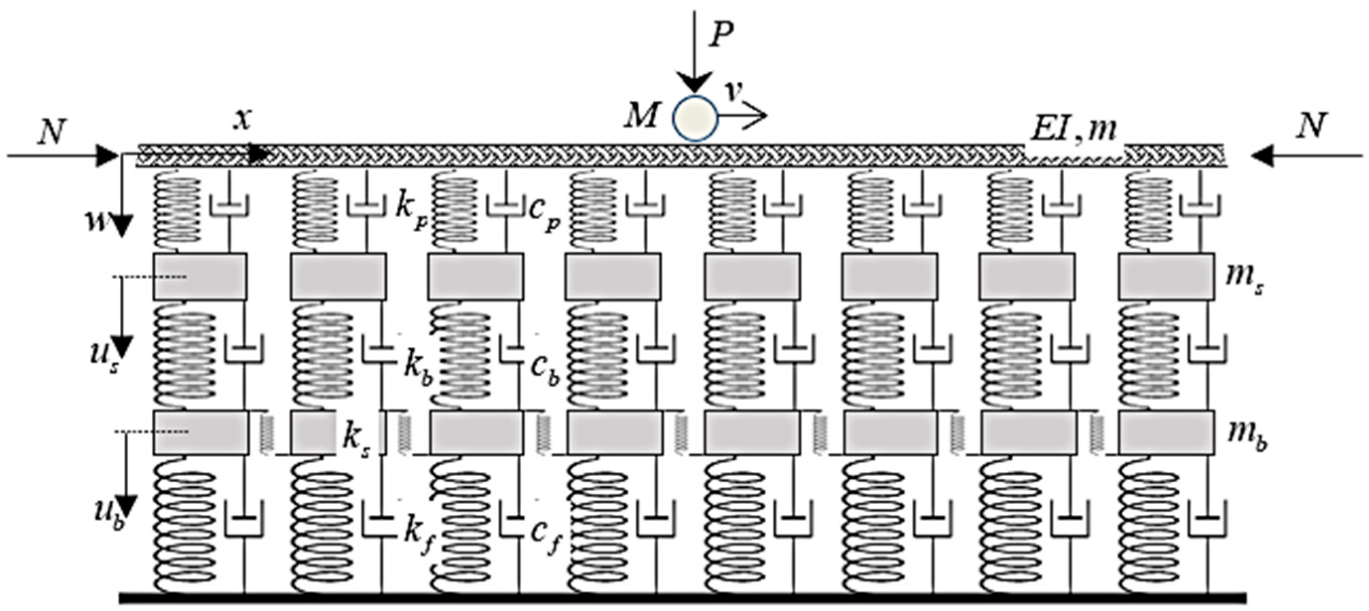
The three-layer railway track model is quite popular, due to its simplicity, easy manipulability, computational efficiency, and good agreement with reality [17]. It is schematically presented in Figure 1 [18].

To facilitate the analytical steps of the solution, all the parameters are introduced into the governing equations in their distributed and dimensionless forms. Exploiting its symmetry, the model represents a half-track of a single-line straight section.

The governing equations in regard to the dimensionless parameters and moving coordinates read as (more details can be found in [18]):

$$\begin{array}{l}{\tilde{w}}_{,\xi \xi \xi \xi }+4\left({\tilde{w}}_{,\tau \tau }-2\alpha {\tilde{w}}_{,\xi \tau }+{\alpha }^2{\tilde{w}}_{,\xi \xi }\right)+4{\eta }_N{\tilde{w}}_{,\xi \xi }+8{\eta }_p\left({\tilde{w}}_{,\tau }-\alpha {\tilde{w}}_{,\xi }-{\tilde{u}}_{s,\tau }+\alpha {\tilde{u}}_{s,\xi }\right)\\ +4{\kappa }_p\left(\tilde{w}-{\tilde{u}}_s\right)=\left(8{\eta }_P-4{\eta }_M{\tilde{w}}_{,\tau \tau }\right)\delta \left(\xi \right)\end{array}$$

(1)

$$\begin{array}{l}{\mu }_s\left({\tilde{u}}_{s,\tau \tau }-2\alpha {\tilde{u}}_{s,\xi \tau }+{\alpha }^2{\tilde{u}}_{s,\xi \xi }\right)-2{\eta }_p\left({\tilde{w}}_{,\tau }-\alpha {\tilde{w}}_{,\xi }-{\tilde{u}}_{s,\tau }+\alpha {\tilde{u}}_{s,\xi }\right)\\ -{\kappa }_p\left(\tilde{w}-{\tilde{u}}_s\right)+2{\eta }_b\left({\tilde{u}}_{s,\tau }-\alpha {\tilde{u}}_{s,\xi }-{\tilde{u}}_{b,\tau }+\alpha {\tilde{u}}_{b,\xi }\right)+{\kappa }_b\left({\tilde{u}}_s-{\tilde{u}}_b\right)=0\end{array}$$

(2)

$$\begin{array}{l}{\mu }_b\left({\tilde{u}}_{b,\tau \tau }-2\alpha {\tilde{u}}_{b,\xi \tau }+{\alpha }^2{\tilde{u}}_{b,\xi \xi }\right)-{\eta }_s{\tilde{u}}_{b,\xi \xi }-2{\eta }_b\left({\tilde{u}}_{s,\tau }-\alpha {\tilde{u}}_{s,\xi }-{\tilde{u}}_{b,\tau }+\alpha {\tilde{u}}_{b,\xi }\right)\\ -{\kappa }_b\left({\tilde{u}}_s-{\tilde{u}}_b\right)+2{\eta }_f\left({\tilde{u}}_{b,\tau }-\alpha {\tilde{u}}_{b,\xi }\right)+{\tilde{u}}_b=0\end{array}$$

(3)

where

$$\chi =\sqrt[4]{{\displaystyle \frac{k_f}{4EI}}}, v_{ref}=\sqrt[4]{{\displaystyle \frac{4k_{f}EI}{m^2}}}={\displaystyle \frac{1}{\chi }}\sqrt{{\displaystyle \frac{k_f}{m}}}, \alpha ={\displaystyle \frac{v}{v_{ref}}}$$

(4)

$${\mu }_s={\displaystyle \frac{m_s}{l_{s}m}}, {\mu }_b={\displaystyle \frac{m_b}{l_{s}m}}, {\kappa }_p={\displaystyle \frac{k_p}{l_s{k}_f}}, {\kappa }_b={\displaystyle \frac{k_b}{l_s{k}_f}}, {\eta }_s={\displaystyle \frac{k_s{l}_s}{2\sqrt{EI{k}_f}}}$$

(5)

$${\eta }_N={\displaystyle \frac{N}{2\sqrt{EI{k}_f}}}, {\eta }_p={\displaystyle \frac{c_p}{2l_s\sqrt{m{k}_f}}}, {\eta }_b={\displaystyle \frac{c_b}{2l_s\sqrt{m{k}_f}}}, {\eta }_f={\displaystyle \frac{c_f}{2\sqrt{m{k}_f}}}$$

(6)

where $EI$ and $m$ describe the Euler–Bernoulli beam on top of the model, by its bending stiffness and mass per unit length. Further, $l_s$ is the sleeper spacing, $m_s$ and $m_b$ are the masses of the sleeper (half) and ballast cone, and $k_p$, $k_b$, $k_f$, and $k_s$ are the vertical stiffnesses of the rail pads, ballast cone, and foundation, and the shear stiffness of the ballast layer, respectively, where $k_f$ is usually defined as distributed, while the other values are discrete. The ballast cone theory according to [33], and refined in [17,34], is essential in regard to the definition of the governing parameters. $N$ is the axial force and $P$ the vertical force acting on a moving mass $M$ that is traversing the model at a constant velocity $v$. Unknown displacement fields of the beam $w$, the sleeper $u_s$, and the ballast $u_b$ are functions of spatial coordinate $x$ and time $t$. By switching to moving coordinates, $x$ passes to $r=x-vt$ and then to their dimensionless counterparts:

$$\xi =\chi r, \tau =\chi v_{ref}t$$

(7)

further

$${\eta }_M={\displaystyle \frac{M\chi }{m}}, {\eta }_P={\displaystyle \frac{P}{P}}$$

(8)

and the other parameters in Equations (5) and (6) are masses (${\mu }_s$ and ${\mu }_b$), stiffnesses (${\kappa }_p$, ${\kappa }_b$ and ${\eta }_s$), damping ratios (${\eta }_p$, ${\eta }_b$ and ${\eta }_f$), and the axial force ratio (${\eta }_N$). To complete the list of symbols, $\delta$ is the Dirac delta function, and the derivatives are denoted by the symbol of the respective variable, preceded by a comma.

This means that a Winkler beam, characterized by $EI$, $m$, and $k_f$, is selected as the reference beam. Further, $\chi$ is the inverse of its characteristic length, $v_{ref}$ is the critical velocity of a moving force, and $\alpha$ is, therefore, the velocity ratio. For the identification of the moving mass instability, it is assumed that the mass is always in contact with the beam. Finally,

$$w_{ref}={\displaystyle \frac{P\chi }{2k_f}}, \tilde{w}={\displaystyle \frac{w}{w_{ref}}}, {\tilde{u}}_s={\displaystyle \frac{u_s}{w_{ref}}}, {\tilde{u}}_b={\displaystyle \frac{u_b}{w_{ref}}}.$$

(9)

Considering the range of admissible parameters specified in detail in [34], it is possible to conclude that the admissible ranges of the leading parameters are approximately as follows:

$${\mu }_s\in 〈1;6〉, {\mu }_b\in 〈2;45〉, {\kappa }_p\in 〈0.03;4.2\times {10}^4〉, {\kappa }_b\in 〈0.04;6\times {10}^3〉$$

(10)

Nevertheless, it is also necessary to point out that there are general trends, such as enlarging sleeper spacing, the introduction of novel lightweight materials, and other cost-saving measures, which can obviously affect these ranges.

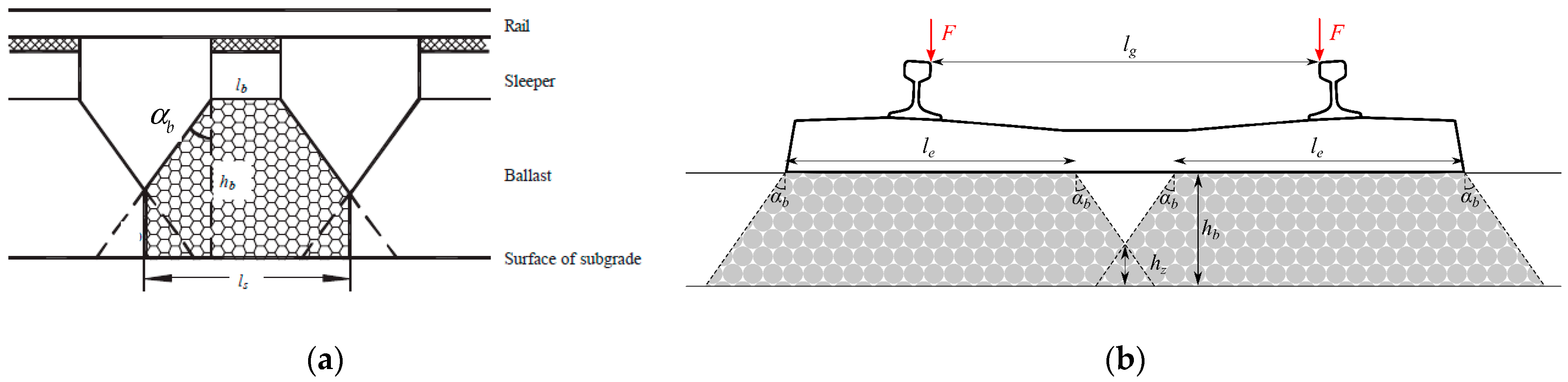
The admissible intervals in Equation (10) were obtained in the following way: First, geometrical data needed for the stress cone theory were assumed as:

$$l_s=〈0.5;0.8〉, h_b=〈0.2;0.6〉, l_b=〈0.2;0.36〉, {\alpha }_b=〈{25}^{\mathrm{o}};{50}^{\mathrm{o}}〉$$

(11)

All the values except for ${\alpha }_b$ are given in [m]. Further, $h_b$, $l_b$, and ${\alpha }_b$ are the ballast height, base sleeper width, and angle of the ballast cone, as exemplified in Figure 2 [17].

Further, $l_g$ and $l_e$ are the rail gauge and the sleeper effective length. For the calculations, $l_e=1 \mathrm{m}$ is used as the most common value and, so, $l_g$ does not have to be introduced. Then, by using the ranges from Equation (11), the dynamically activated ballast volume $m_{cn}$ is within the range (0.065–0.7) m³, and the parameter related to the vertical stiffness $k_{cn}$ falls within the range (0.79–3.36) m (multiplication by the ballast Young’s modulus yields the correct base unit of N/m). According to [17,18], the range (40–160) kg is considered for $m_s$, and the ballast density ${\rho }_b$ is taken to be within the range (1200–2600) kg/m³. Further, values within the range (20–5000) MN/m are considered for $k_p$ and (50–400) MPa for the ballast Young’s modulus, $E_b$.

There is an obvious connection between ${\mu }_s$ and ${\mu }_b$, as well as between ${\kappa }_p$ and ${\kappa }_b$, as they are both connected to the reference beam. Their ratios must be bounded by the values determined as:

$${\left({\displaystyle \frac{{\mu }_s}{{\mu }_b}}\right)}^{+}={\displaystyle \frac{m_s^{+}}{m_{cn}^{-}{\rho }_b^{-}}}={\displaystyle \frac{160}{0.065\cdot 1200}}=2.05, {\left({\displaystyle \frac{{\mu }_s}{{\mu }_b}}\right)}^{-}={\displaystyle \frac{m_s^{-}}{m_{cn}^{+}{\rho }_b^{+}}}=0.022$$

(12)

$${\left({\displaystyle \frac{{\kappa }_p}{{\kappa }_b}}\right)}^{+}={\displaystyle \frac{k_p^{+}}{k_{cn}^{-}{E}_b^{-}}}={\displaystyle \frac{5\times {10}^9}{0.79\cdot 5\times {10}^7}}=126.58, {\left({\displaystyle \frac{{\kappa }_p}{{\kappa }_b}}\right)}^{-}={\displaystyle \frac{k_p^{-}}{k_{cn}^{+}{E}_b^{+}}}={\displaystyle \frac{2\times {10}^7}{3.36\cdot 4\times {10}^8}}=0.015$$

(13)

In what follows, “+” and “–“ will be used to identify the upper and lower bounds, respectively.

Additionally, it will be demonstrated that graphical representation in logarithmic scale for ${\kappa }_p$ and ${\kappa }_b$ is more advantageous, as was already used in [18,29]. For the analysis in this paper, the full range does not have to be covered; thus, the following representation is proposed:

$${\kappa }_p=0.03\times {10}^{\left(in{d}_p-1\right)0.05}, {\kappa }_b=0.04\times {10}^{\left(in{d}_b-1\right)0.05}$$

(14)

According to which, for the ratios from Equation (13), defines a range for the difference between the indexes, $in{d}_p$ and $in{d}_b$:

$${\displaystyle \frac{{\kappa }_p}{{\kappa }_b}}=0.75\times {10}^{\left(in{d}_p-in{d}_b\right)0.05}, -34.05\le \left(in{d}_p-in{d}_b\right)\le 44.55$$

(15)

3. Methods

3.1. Terminology

This subsection clarifies the adopted terminology. The moving force problem is defined as a longitudinally homogeneous supporting structure, which is traversed by a constant force at a constant velocity. In such a case, the transient part of the solution is not very important, and if a steady-state solution exists, it is rapidly attained.

In this context: the critical velocity (CV) designates a velocity fulfilling the following four conditions:

(i)

It marks a true resonance, meaning that when the force moves at this velocity, deflections tend toward infinity in the undamped case (i.e., the steady-state solution is never reached);

(ii)

This velocity marks a local minimum of the generalized mode number of an equivalent finite beam;

(iii)

There is a sudden jump to zero deflection at the active point (AP) at a velocity infinitesimally higher;

(iv)

The CV value separates regions of instability in regular cases.

On the other hand, the false critical velocity (FCV), which is also a true resonance, marks a local maximum of the generalized mode number of an equivalent finite beam and has no influence on instability regions or the specific value at the AP.

In the three-layer model, as the three layers indicate, three CVs are expected, which means five resonances occur in the moving force problem: three corresponding to CVs and two to FCVs. In a regular case, there are five vertical asymptotes of the instability lines. Four of them are confining two instability line branches in the first two regions, delimited by the CVs. After that, the third and final instability line branch has the fifth vertical asymptote on the left side and the other end tends toward zero moving mass for an infinite velocity [18,29].

Nevertheless, there are several exceptional cases. In fact, the number of resonances can only be odd: 1, 3, or 5. When there are 5 resonances, they are divided into 3 CVs and 2 FCVs. When this number is less than 5, some FCVs do not exist, and CVs are replaced by pseudo-critical velocities (PCVs). Namely, 3 resonances indicate 2 CVs, 1 FCV, and 1 PCV; 1 resonance always corresponds to a CV and, so, there are 2 PCVs. Additionally, some cases at the boundary of the separation regions can lead to the merging of some values and a model can exhibit a maximum of 3 resonances (instead of 5).

As already mentioned, when CVs are missing, they are replaced by PCVs. A PCV marks a peak in the vibrations, but not an infinite value. Since no resonance occurs, even in the absence of damping, the deflections never reach infinity. Unlike CVs, FCVs are never replaced, but they can be absent.

The determination of resonances can be conducted semi-analytically, as described in [29], but high precision must be implemented. It is extremely important to perform such determinations in the absence of damping, which can unequivocally distinguish a vibration peak from a true resonance. Many methods used by other authors, such as Green’s function method, require damping for numerical stability and are, therefore, unsuitable.

PCVs can be determined using parametric analyses by extracting the maximum value at the AP and the global maxima and minima over the entire beam. However, when these peaks are hardly visible, the PCV value is ambiguous. This means that the peak at the AP and the global maxima and minima are attained at different velocities and, therefore, it is not clear which of these values should be designated as the PCV. Numerical precision is also essential here. However, even if the calculation must be conducted without damping, MATLAB can be used because the roots required for calculating the steady-state shape can be separated into those defining propagating and evanescent waves. Evanescent waves can be analyzed for extreme deflection values only in the vicinity of the AP. Propagating waves affect the whole beam and, thus, the extraction of extreme values would be time consuming. However, knowing the roots, it is possible to calculate the amplitudes and establish an analytical envelope function that can unequivocally identify the maximum and minimum over the entire beam, without enlarging the tested region around the AP.

Namely, as our interest lies in the initial region of $\alpha$, then when ${\eta }_s=0$, there are two pairs of real roots and four complex roots symmetrically covering the four quadrants. Negligible damping can be introduced to correctly separate the real roots forming the wave ahead of and behind the AP. The four real roots define two harmonic waves, with a constant amplitude and zero phase. It is then possible to calculate the envelope function, which has clearly defined maximum and minimum values over the entire beam. It is then only necessary to check whether, in the vicinity of the AP, these values are exceeded due to evanescent waves. When ${\eta }_s\ne 0$, there is only one harmonic wave, so the amplitude is easily determined, and the use of an envelope function is unnecessary.

In the previous text, the term instability line was used. This relates to the instability of moving inertial objects. In such an analysis, the transient part of the solution is essential, without it, the problem of instability would remain hidden. Instability is not a resonance-type phenomenon; there is a velocity interval within which the object becomes unstable. At the extremities of this interval, the object remains stable, and instability is verified only within this interval. This is characterized by an exponential increase in vibration amplitudes. Thus, although the steady-state solution usually exists and is finite, it is never reached.

Instability is determined by solving the roots of the characteristic equation. The roots always come in pairs, identifying the harmonic parts of the full solution. When this part grows exponentially, the roots are termed unstable. The instability line is traced in the ($\alpha$ − ${\eta }_M$) plane as a boundary between regions with a different number of unstable roots. In this paper, only one moving mass is considered. For this case, for a selected $\alpha$, it is possible to track real-valued frequencies until a real-valued equivalent stiffness (or flexibility) of the supporting structure is detected; then, ${\eta }_M$ is calculated using the characteristic equation. In this way, the analysis remains in the real domain, and the D-decomposition method, used by other researchers, can be avoided.

3.2. Determination of the Number of Resonances and Pseudo-Critical Velocities

Although the admissible range of dimensionless parameters is known, analytically identifying regions corresponding to a specific number of resonances remains challenging. However, it is relatively easy to calculate the number of resonances semi-analytically for a particular case using software with adaptable precision (e.g., Maple or Mathematica). MATLAB is not convenient in this context, as damping should not be included and high precision in root determination is required.

The number of resonances is always odd, 1, 3, or 5, corresponding to 1, 2, or 3 critical velocities (CVs), and 0, 1, or 2 false critical velocities (FCVs), as explained in the previous section.

Four selected cases are shown as a demonstration in Figure 3. It was found to be convenient to select ${\mu }_s$, ${\mu }_b$, and ${\eta }_s$, or, alternatively, ${\eta }_N$, and to use the logarithmic scale for ${\kappa }_p$ and ${\kappa }_b$, as indicated in Equation (14). This means that both indexes, $in{d}_p$ and $in{d}_b$, were selected for the semi-analytical determination from discrete values ranging from 1 to 101 in increments of 1.

As already mentioned, these graphs can only be obtained semi-analytically using Maple or a similar software, because MATLAB does not provide sufficient accuracy to determine the roots, which is essential.

Once the number of resonances is known, in cases where this number is less than 5, the PCV(s) must be determined. It can be verified that they are often lower than the first resonance. In such cases, the lowest PCV plays the role of a critical velocity for track design. Hence, it can be termed the design critical velocity (DCV).

PCVs, which can be determined using parametric analysis, may be well-pronounced or ambiguous. In well-pronounced cases, the peak at the AP and the global maxima and minima over the entire beam are achieved at the same $\alpha$, which is not true in ambiguous cases. The following figures explain these issues graphically. The case presented in Figure 3d is selected first. Then, in addition to ${\mu }_s=4$, ${\mu }_b=12$, and ${\eta }_s=1$ (${\eta }_N=0$), and $in{d}_b=21$, $in{d}_p=31;41;51$ are used to identify cases with 1, 3, and 5 resonances.

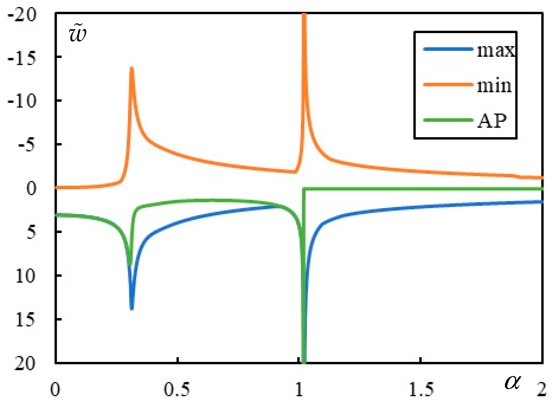
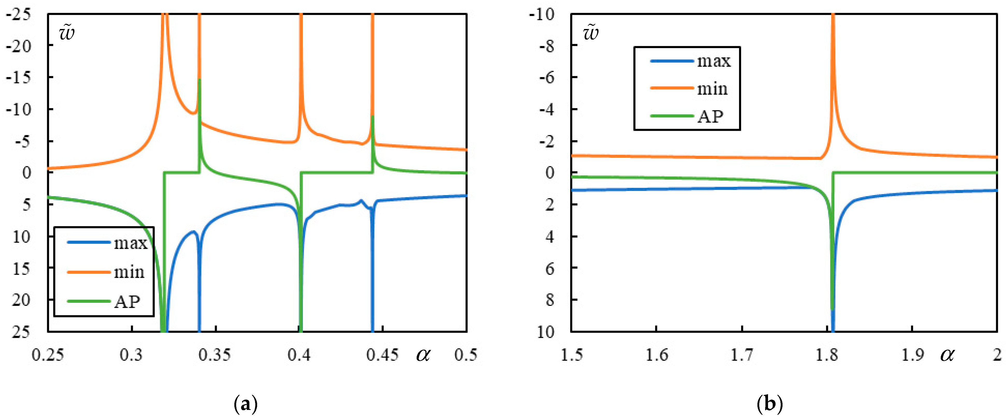
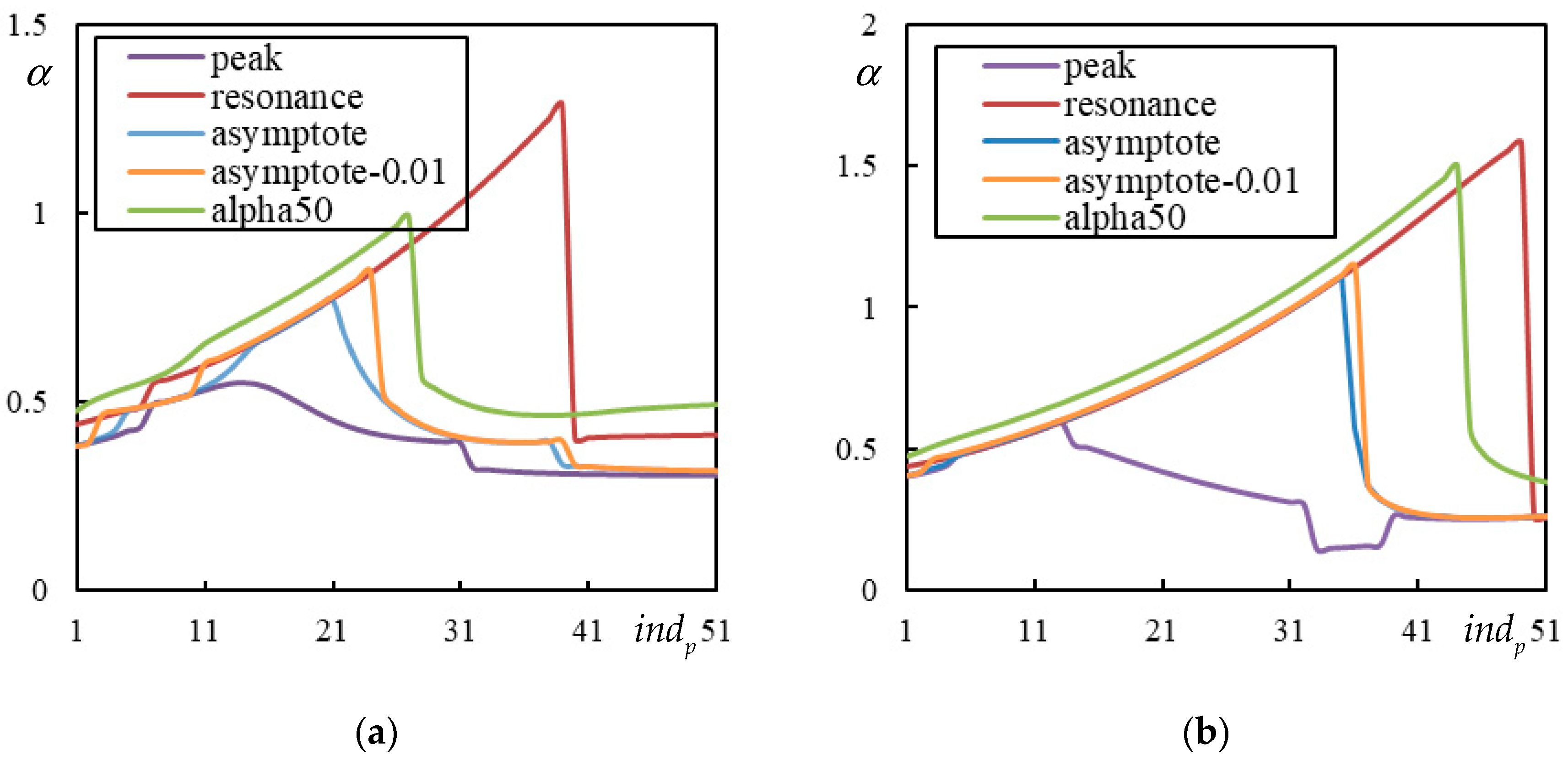
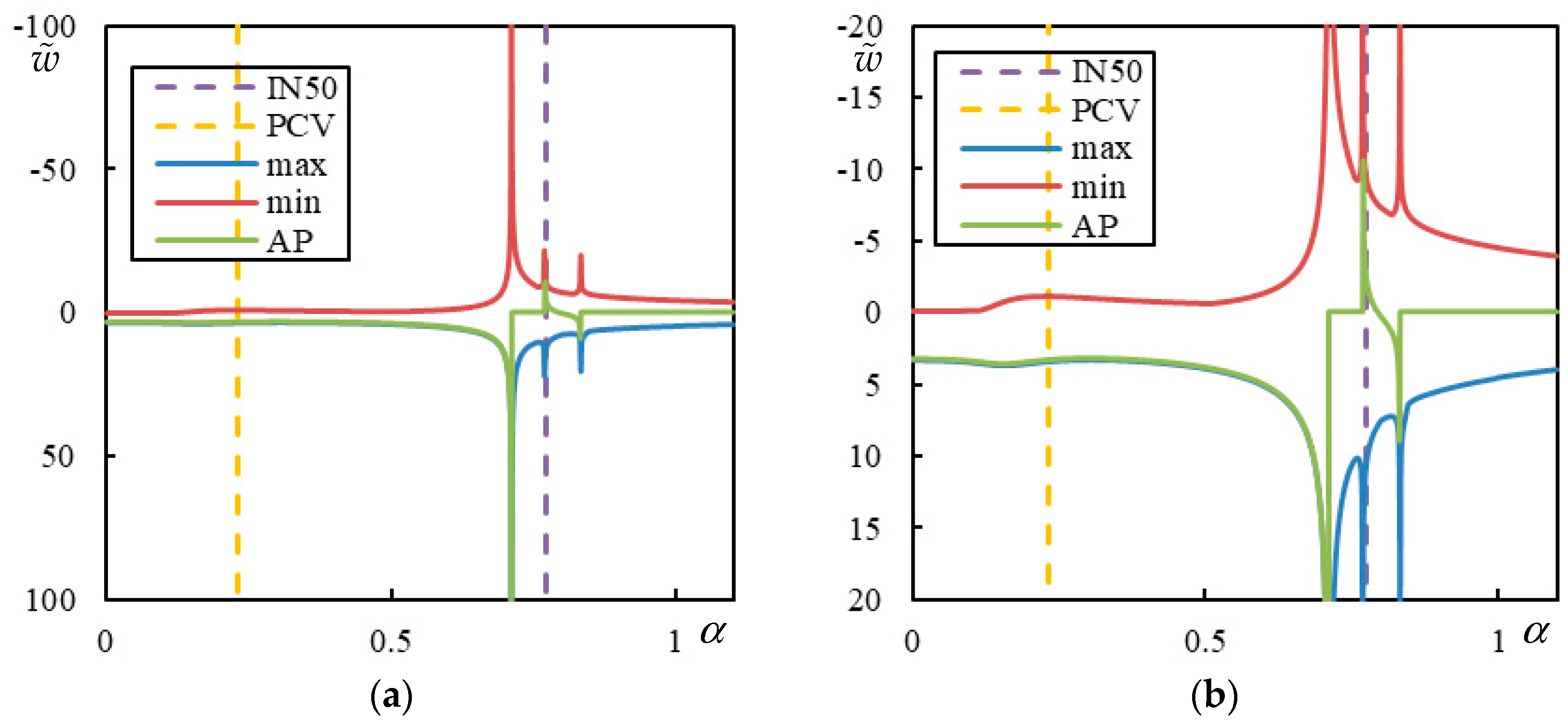
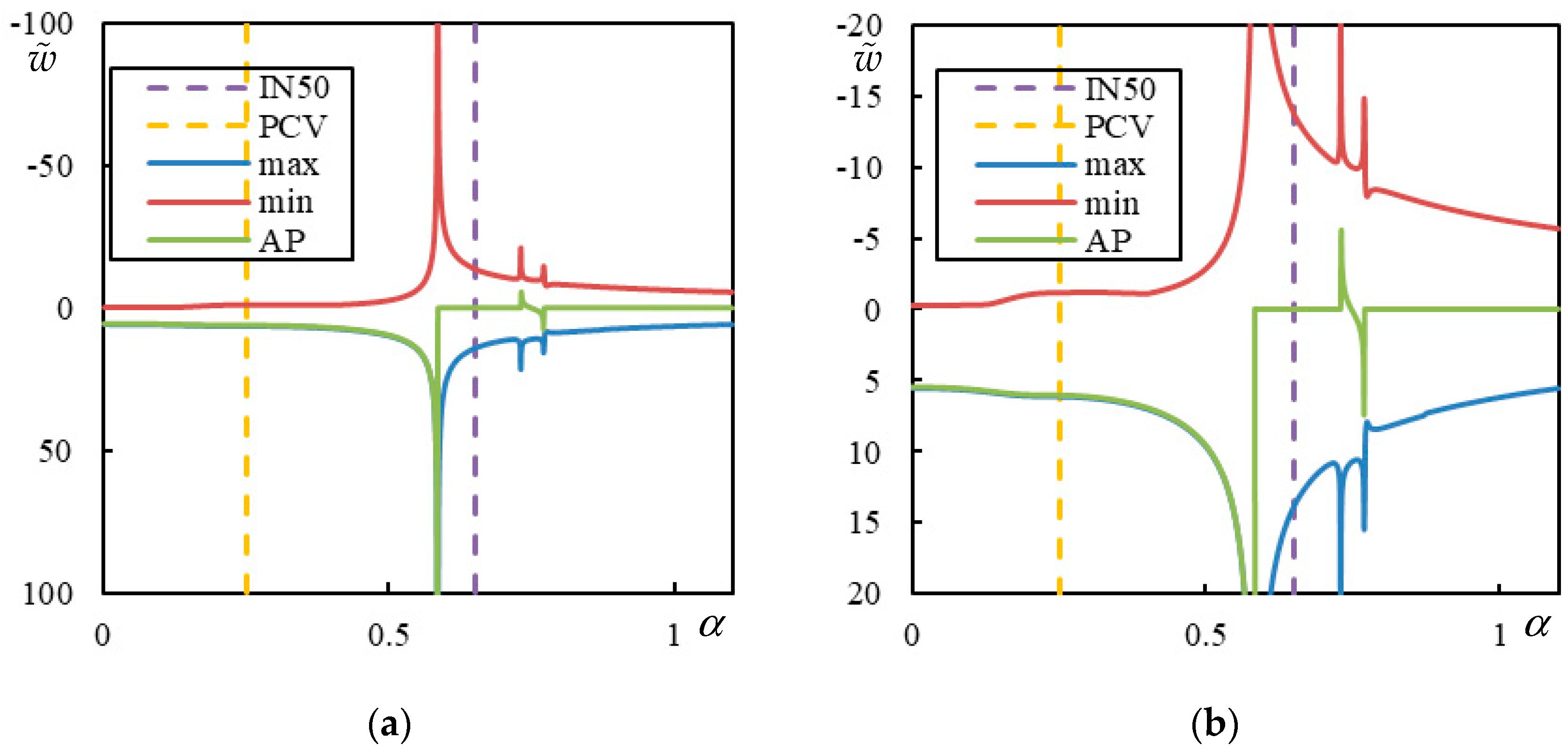
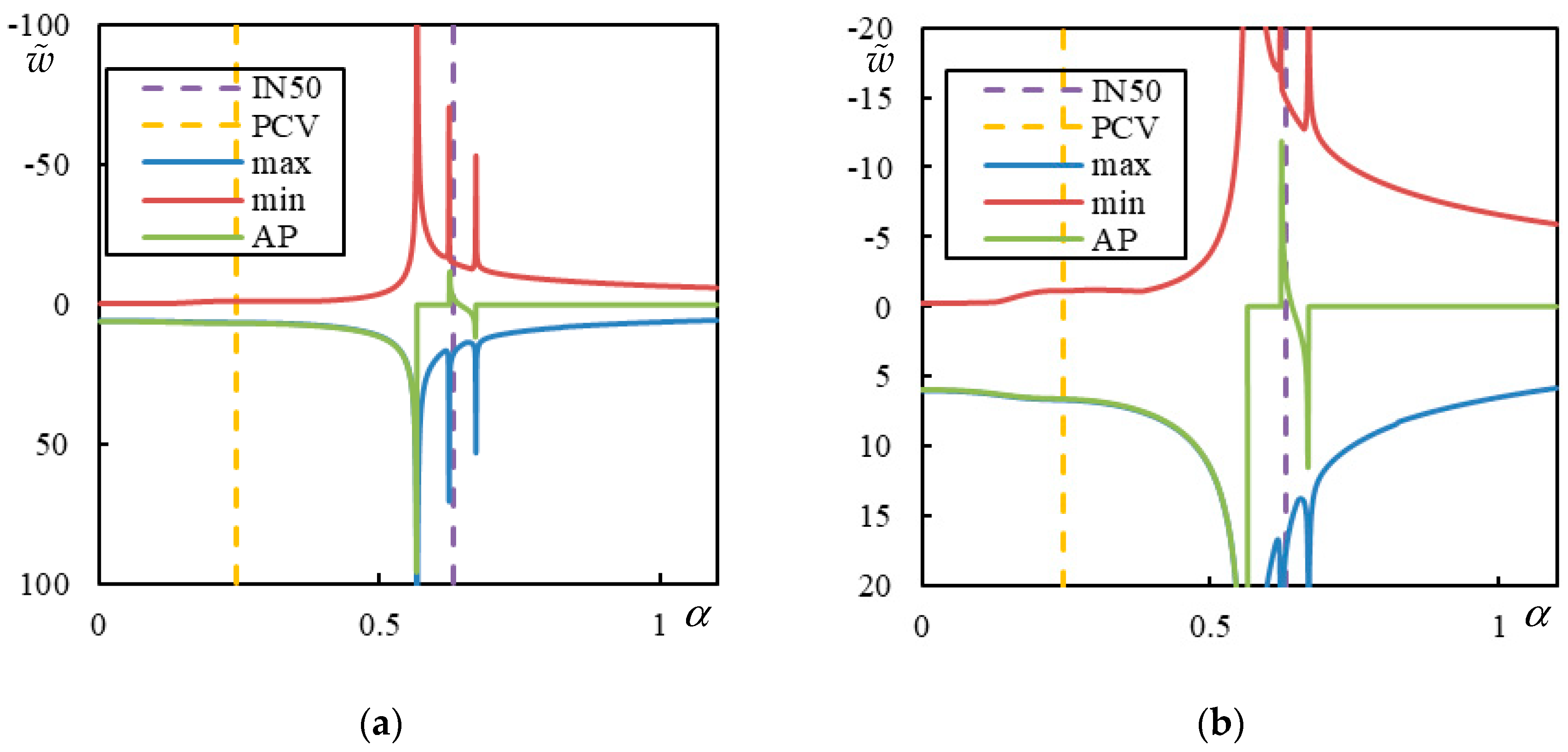
In Figure 4, the case with 1 resonance is shown. This is an exceptional case characterized by a maximum of 3 resonances. Since only one resonance is present, the FCV is absent. The PCV is relatively well-pronounced at $\alpha =0.310$ for both the maximum and minimum over the whole beam, while the peak at the AP occurs at $\alpha =0.303$. These values are determined with a precision of 0.001, which corresponds to the step size used in the parametric analysis. Resonance occurs at $\alpha =1.016877$.

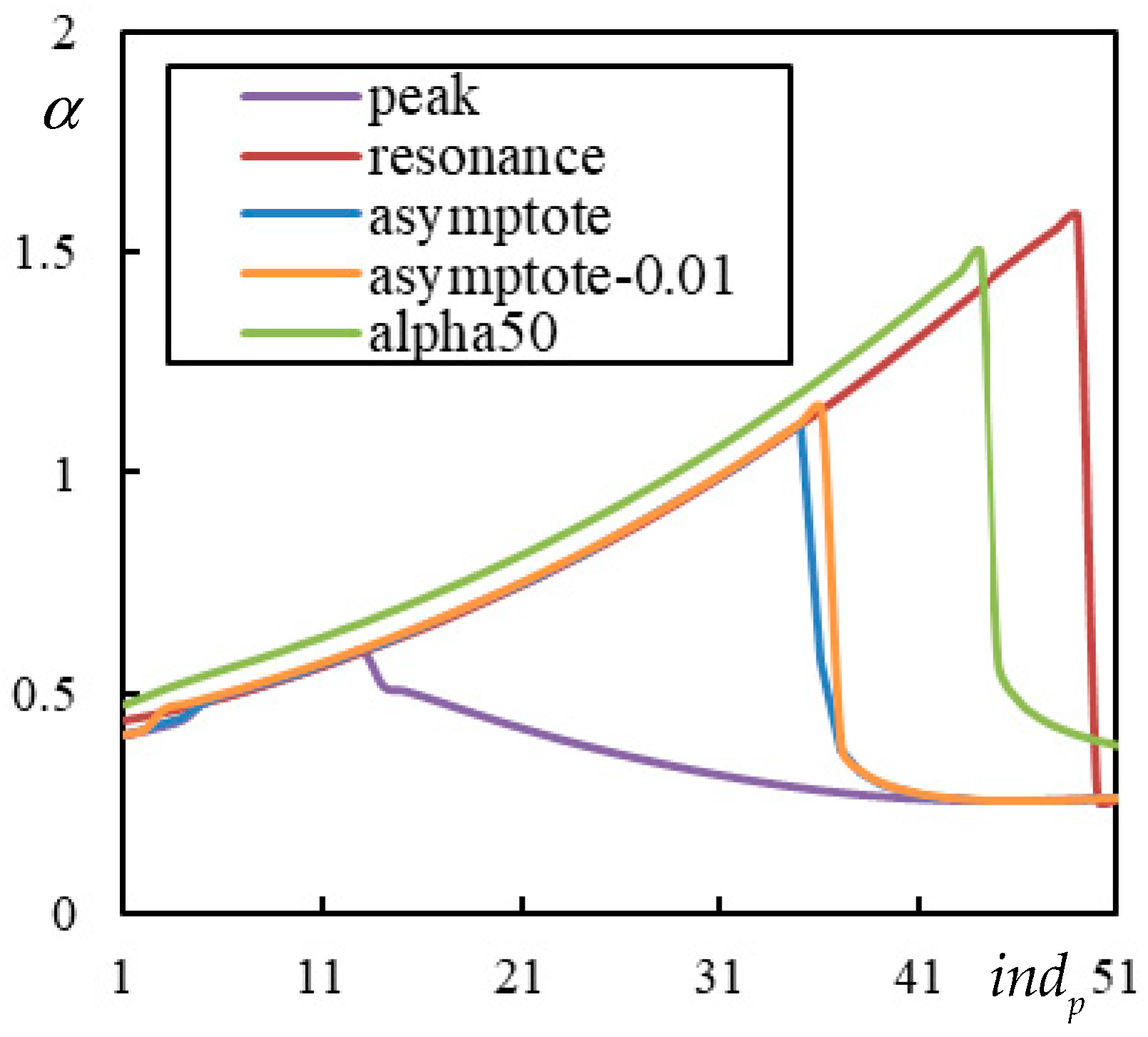
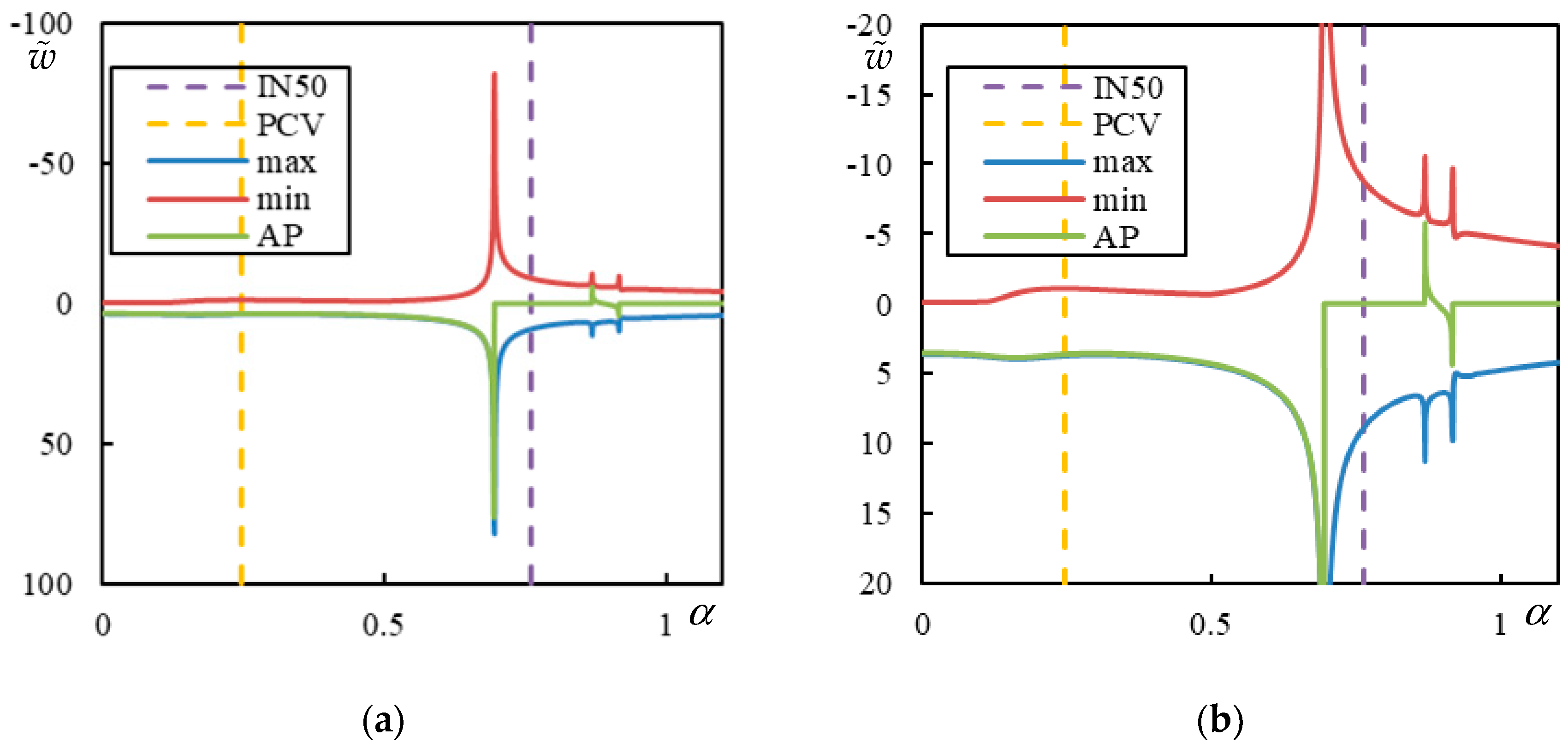
In Figure 5, the case with 3 resonances is shown. Two CVs are clearly marked by a sudden jump to zero at the AP: $\alpha =0.317124$ and $\alpha =1.354864$. Then, $\alpha =0.327508$ is the FCV. There is also a barely visible PCV, with peaks at $\alpha =0.3792$ for the maximum and minimum over the whole beam, while the peak at the AP occurs at $\alpha =0.3706$. These values are determined with a precision of 0.0001, which is the step size used in the parametric analysis.

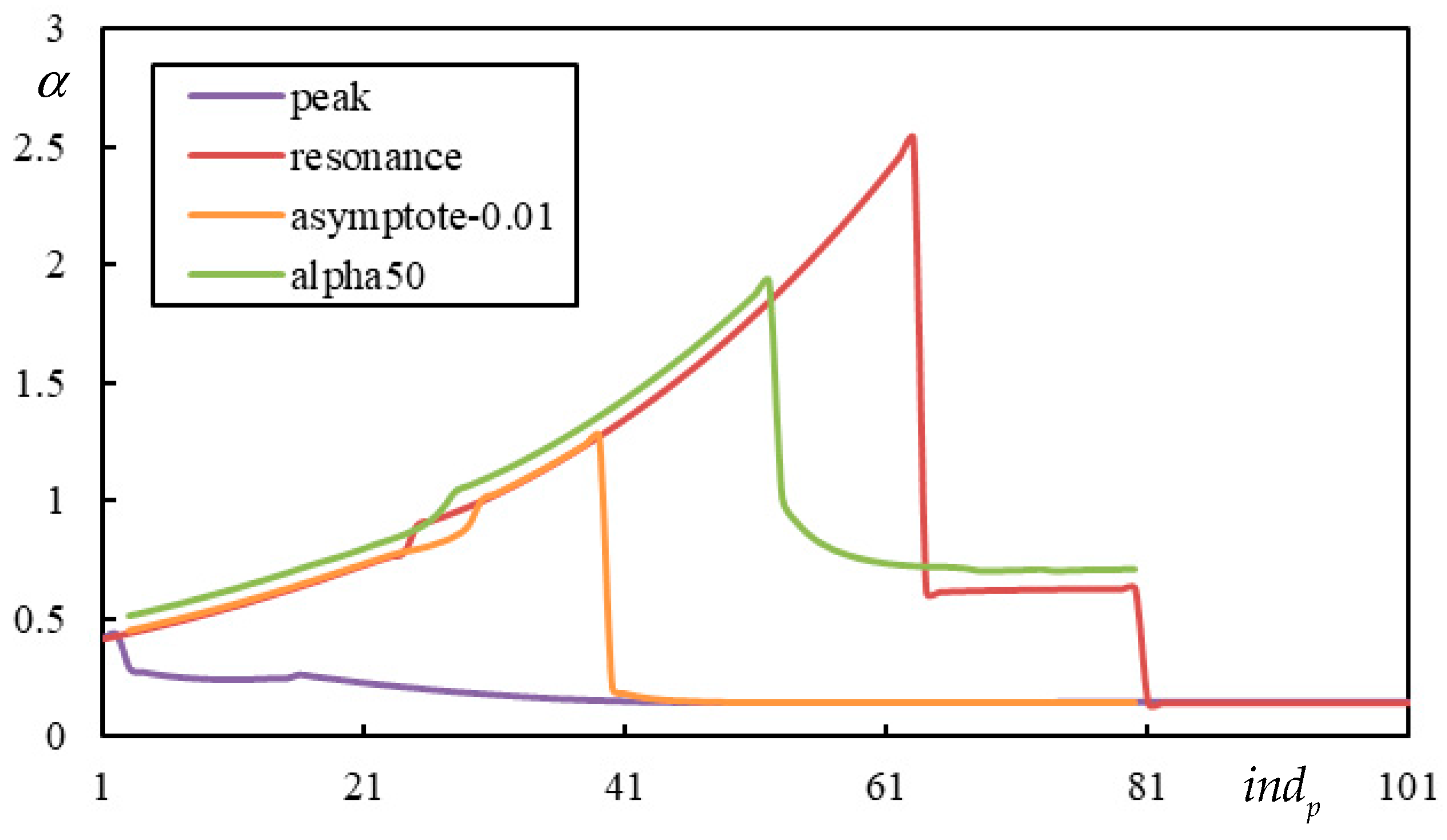
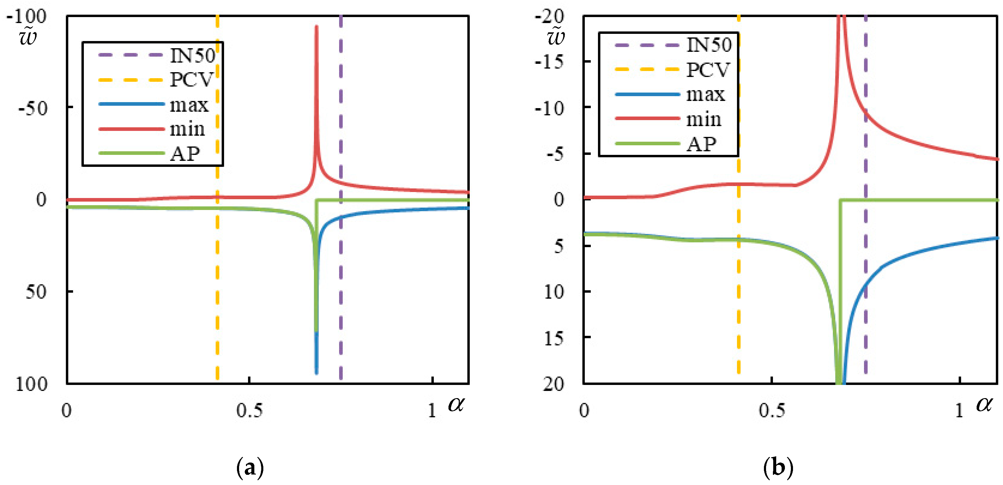
Finally, in Figure 6, the case with 5 resonances is shown. Three CVs are clearly marked by a sudden jump to zero at the AP: $\alpha =0.319163$, $\alpha =0.400814$, and $\alpha =1.806272$. Between them, two FCVs occur: $\alpha =0.340119$ and $\alpha =0.443505$. There are no indications of other vibration peaks.

Several other cases are included in [18,29].

Due to the challenges in determining the PCV, first, the necessity of parametric analysis instead of semi-analytical methods and, second, the ambiguity in identifying clear peaks, it is worthwhile to explore other possibilities. In Figure 5, at least, the maxima and minima over the beam occurred at the same $\alpha$, but this is not always the case. Therefore, the PCV can be ambiguous when the peaks do not coincide.

Since the PCV replaces the CV in separating the instability regions, it is natural to propose that it should be predicted by $\alpha$, which indicates a vertical asymptote in the instability line. This newly proposed approach exploits the regularity of the single moving mass problem, exemplified by the one-layer model in Figure 7.

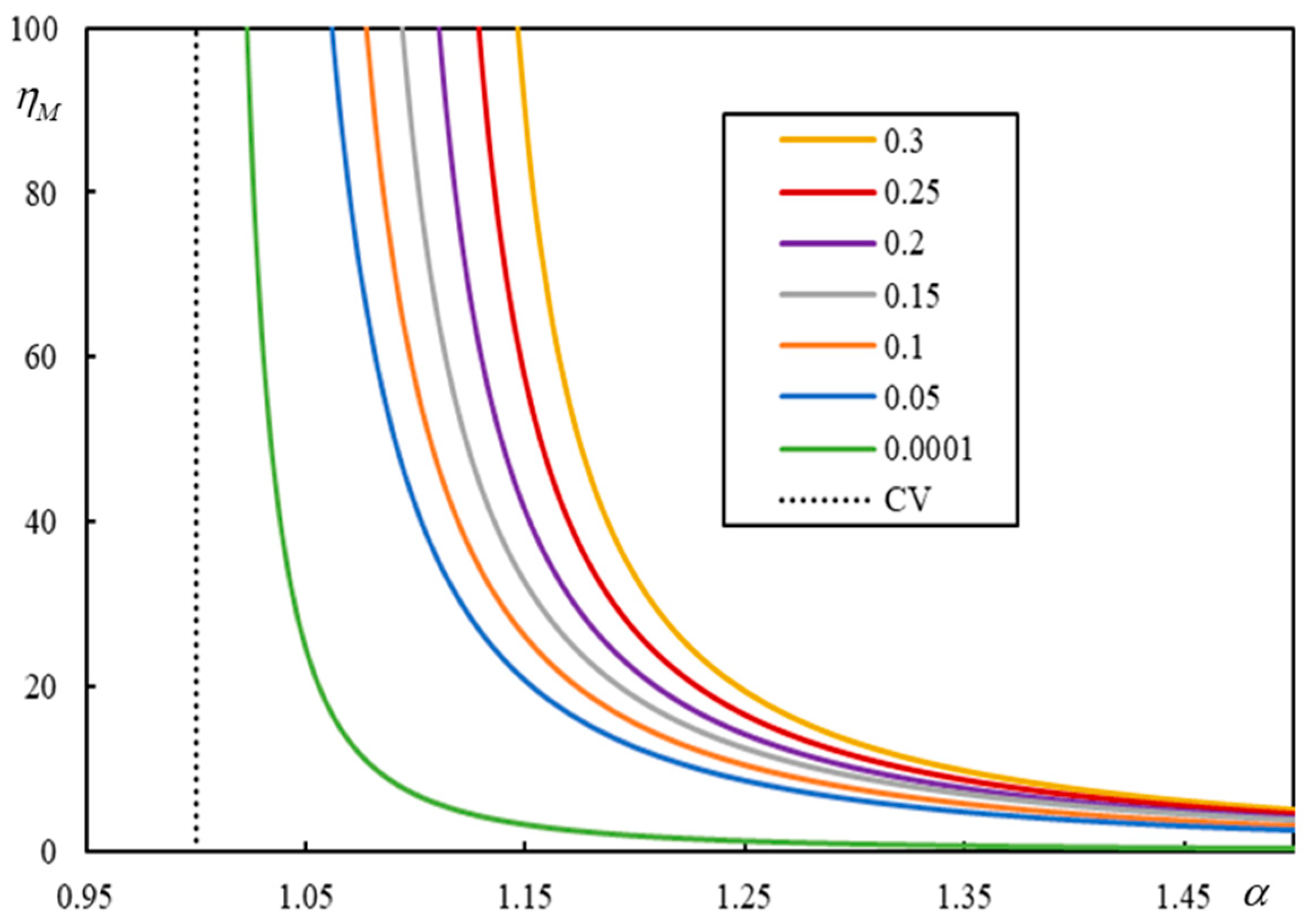
It is demonstrated in Figure 7 that, as the damping ratio decreases, the instability lines approach the CV. Therefore, a very good estimate of the CV can be obtained by identifying the onset of instability for infinitely low damping. Such calculations can be performed semi-analytically in software with adaptable number of digits used for calculation. Infinitely low damping and an infinitesimally small real-valued frequency are used to find an $\alpha$-value leading to a real-valued equivalent stiffness (or flexibility). The corresponding ${\eta }_M$ tends toward infinity.

Applying the same reasoning to the three-layer model, it should be possible to identify the lowest PCV. This was tested for the case shown in Figure 3a, with ${\mu }_s=1$, ${\mu }_b=2$, and ${\eta }_s=0$. In Figure 8a, $in{d}_b=26$ and, in Figure 8b, $in{d}_b=29$. The latter case is the only one where the region of 3 resonances extends fully, and 5 resonances occur only at the very beginning.

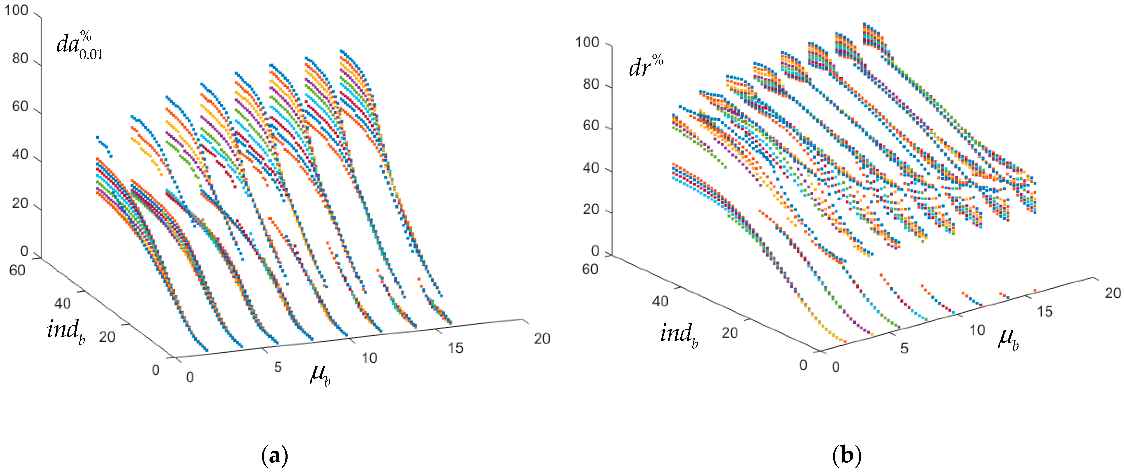
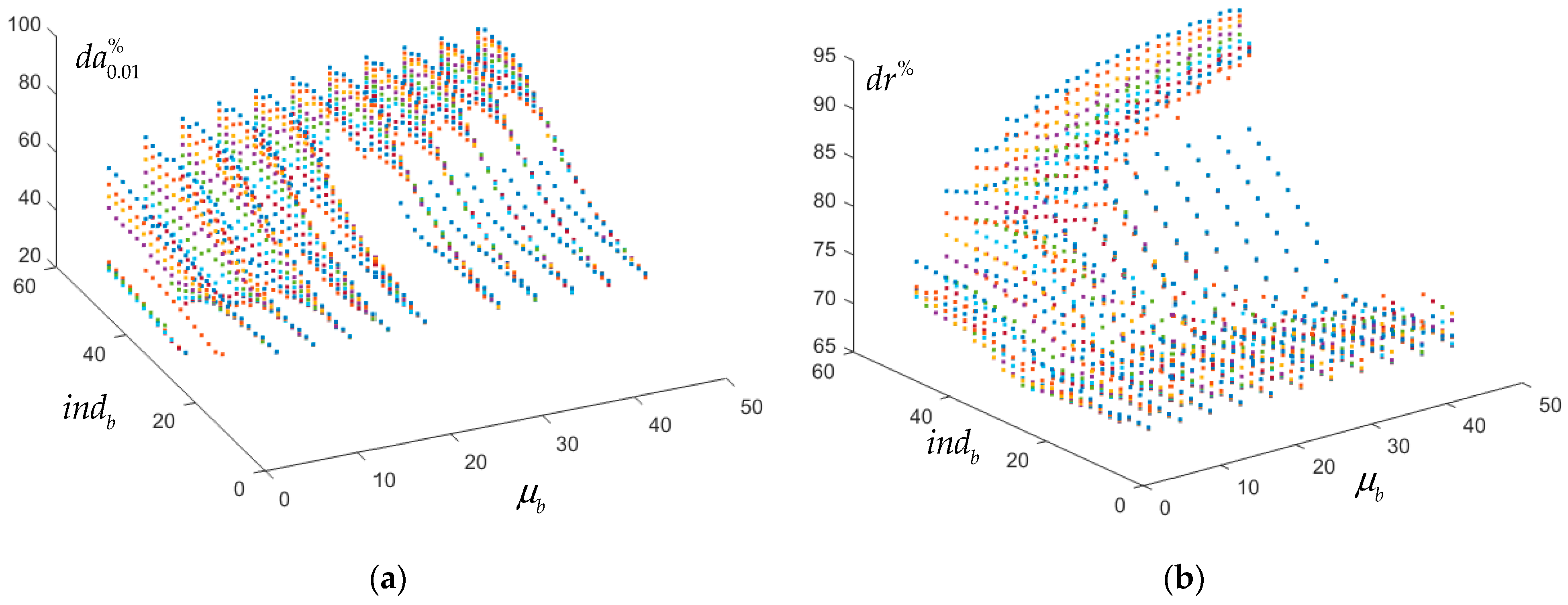
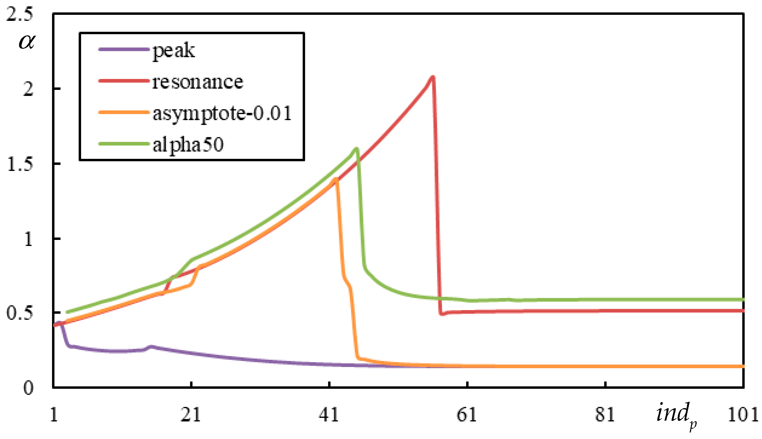
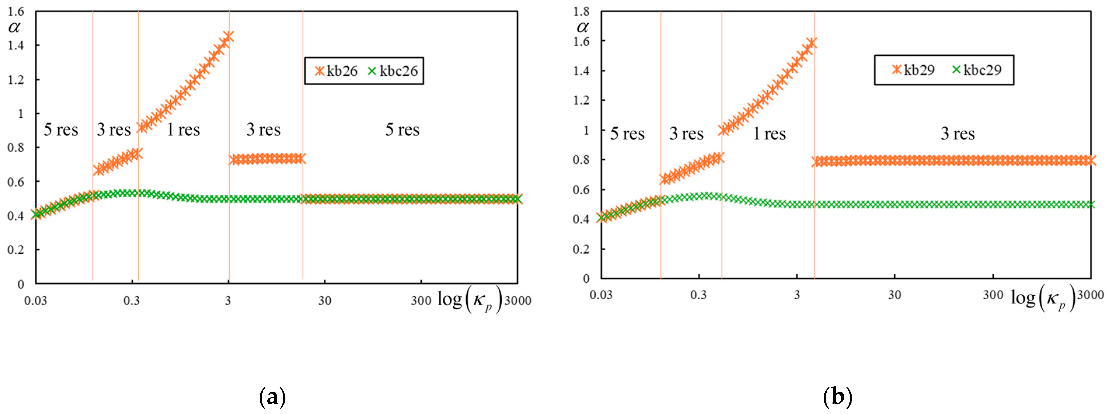
It can be concluded from Figure 8 that the PCV identification works well: the line of green crosses is smooth, as expected. In regions with 5 resonances, the crosses coincide, while, in other regions, the green crosses indicate a much lower value. Nevertheless, there are cases, as already mentioned, where the maximum number of resonances is only 3. 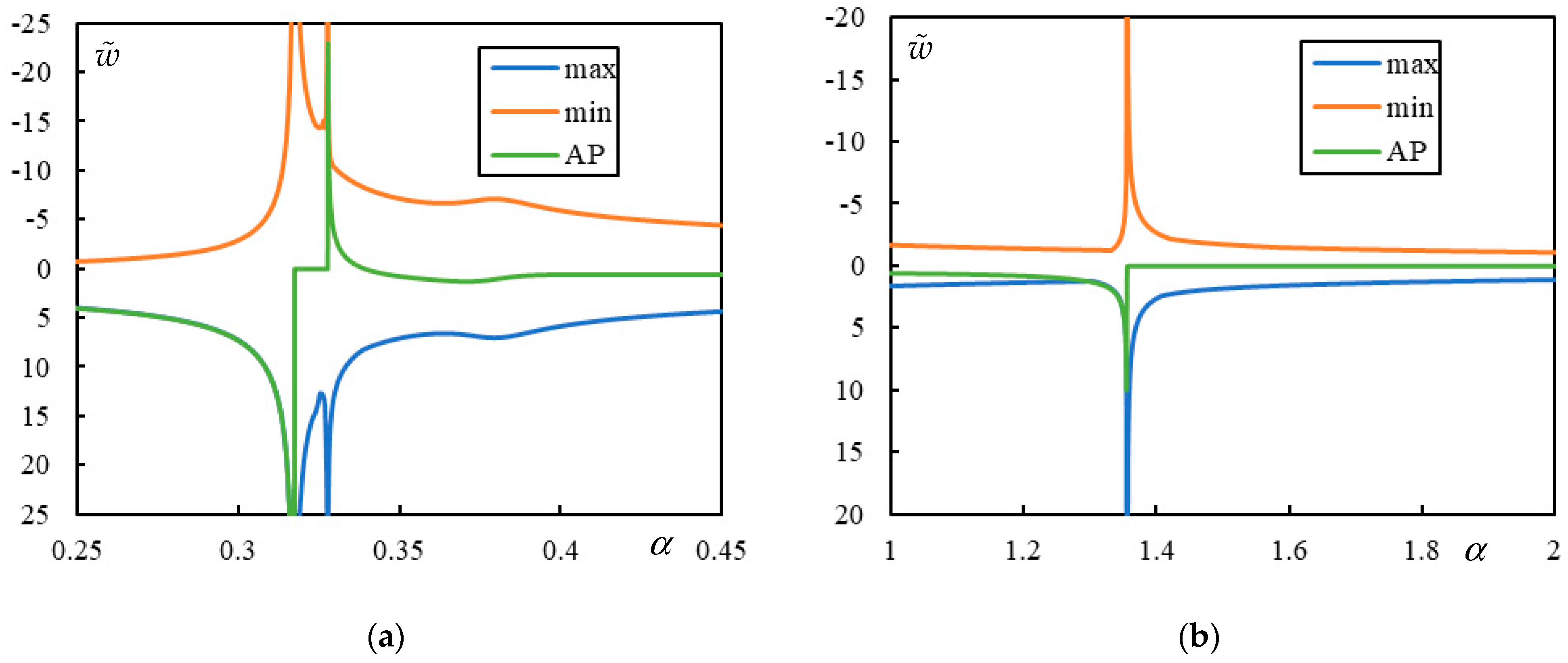Then, the crosses match in the region of 3 resonances, as shown in Figure 9, where the results of the parametric analysis are also included to show that no additional peaks occur (higher velocities were also tested). The graph in part (a) is plotted only up to $in{d}_p=34$ for clarity.

In Figure 9b, the resonances are 0.339502, 0.377294, and 0.816655, corresponding to the CV, FCV, and CV, respectively. The lowest asymptote is at $\alpha =0.339502$, which perfectly matches the lowest resonance. This shows that the proposed technique works well in most cases. However, there are exceptions, where the lowest PCV is lower than the lowest asymptote. These cases are, in fact, the focus of this paper.

This section concludes by illustrating the effect of the PCV, CV, and FCV on instability lines in typical cases. When there are five resonances, three of them correspond to CVs and two to FCVs. Five vertical asymptotes of the instability lines then appear, defining two full branches in the first two regions, delimited by the CVs. Beyond that, the final branch tends toward zero ${\eta }_M$ as $\alpha$ approaches infinity. When there are fewer resonances, CVs may be replaced by PCVs. In contrast, FCVs are never replaced and may be absent, as already mentioned.

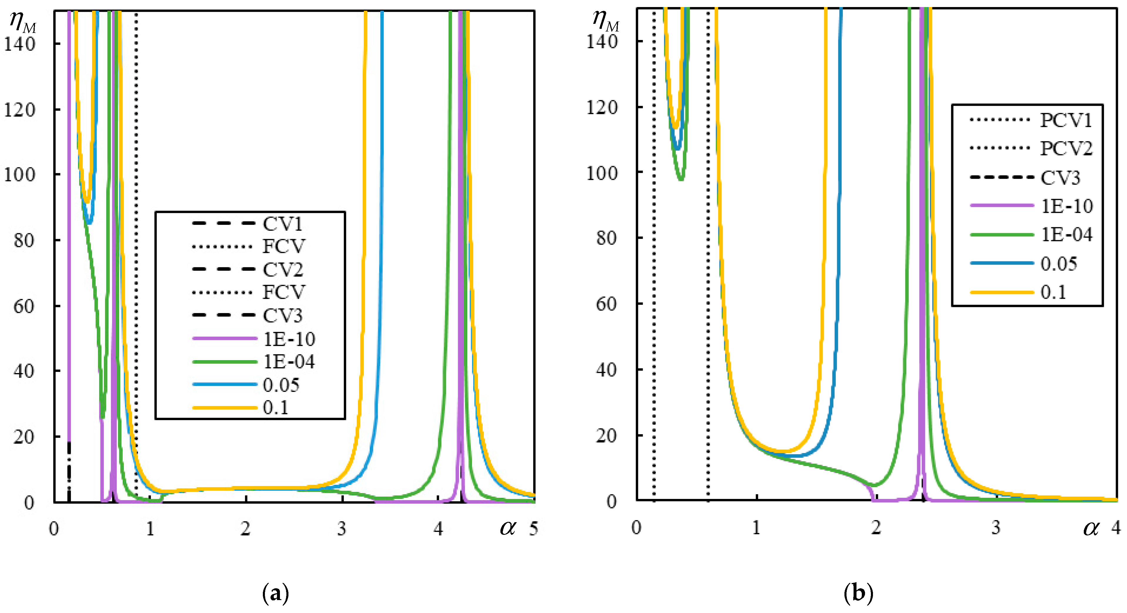
The same cases as previously shown in [18] are selected for demonstration purposes. These cases differ in ${\kappa }_p$, highlighting how this parameter affects the number of resonances. Specifically, both cases have ${\mu }_s=6$, ${\mu }_b=35$, ${\kappa }_b=7$, and ${\eta }_s=0$. For ${\kappa }_p=300$, there are 5 resonances (0.151–CV1; 0.152–FCV; 0.627–CV2; 0.851–FCV; 4.244–CV3). However, for ${\kappa }_p=30$, there is only one (~0.149–PCV1; 0.599–PCV2; 2.388–CV3). This is demonstrated in Figure 10.

It is clear from Figure 10 that the FCV does not influence the separation of instability lines into three distinct regions. It is further shown that PCVs act as CVs, and with decreasing damping, the instability lines approach either the CV or PCV. In the middle region, larger deviations are observed from the right than from the left. To complete this analysis, the corresponding real-valued frequency $q_M$, which gives rise to Figure 10 as a root of the characteristic equation, is plotted in Figure 11.

Figure 11 again demonstrates that as damping decreases, the CV and PCV are approached by vertical asymptotes for which $q_M$ tends toward zero and ${\eta }_M$ tends toward infinity. However, part (b) shows that in the first region, the damping level is not low enough to clearly illustrate this behavior.

An interesting situation occurs when the above-described technique fails, and such an asymptote does not exist. In these cases, only a slight increase in vibration is observed at the PCV. Alternatively, an asymptote may exist, but the instability line covers only unreasonably high ${\eta }_M$ values, so that instability cannot occur. In such cases, circulation velocities can exceed the expected critical velocity.

3.3. Motivation and Aim

As already mentioned, the motivation for this analysis lies in the observation that there are cases where the DCV is a PCV, which is not identified by a vertical asymptote. Thus, it appears possible to tailor the parameters in a way that reduces such vibrations, thereby extending the operational range into the supercritical region.

This suggests that it may be feasible to adjust the parameters of the model using optimization techniques, so that the increase in vibrations remains minimal. As a result, the DCV could be increased without compromising safety. In more detail, the parameters must be adjusted such that the peak at the PCV is minimized, while simultaneously ensuring that the first resonance and the onset of instability for a reasonable value of ${\eta }_M$ and a moderate damping level occur at the highest possible velocity.

Mathematically, the first criterion is defined as the ratio between the highest upward displacement at the DCV = PCV, denoted as $\left|{\tilde{w}}_{\min }^{PCV}\right|$, and the maximum downward displacement in the static case, ${\tilde{w}}_{st}$. The reasoning is twofold: First, because dimensionless displacements are scaled with respect to the static displacement of a reference beam, so it would not be reasonable to use unity for comparison purposes; second, because upward displacements are more critical, they were chosen as the primary criterion.

This criterion is used alongside two others, namely the lowest resonance ${\alpha }_{res}$, and the velocity at the onset of instability ${\alpha }_{m50}$ for a representative mass ${\eta }_M=50$ under a 1% damping ratio, ${\eta }_p={\eta }_b={\eta }_f=0.01$, should be achieved as far as possible. Based on these criteria, the performance index (PI) is defined as:

$$\mathrm{PI}={\displaystyle \frac{\left|{\tilde{w}}_{\min }^{PCV}\right|}{{\tilde{w}}_{st}}}+{\displaystyle \frac{1}{100\min \left(\frac{{\alpha }_{res}-{\alpha }_{PCV}}{{\alpha }_{PCV}},\frac{{\alpha }_{m50}-{\alpha }_{PCV}}{{\alpha }_{PCV}}\right)}}$$

(16)

This PI also serves as the objective function, with the aim of finding its minimum within the admissible domain.

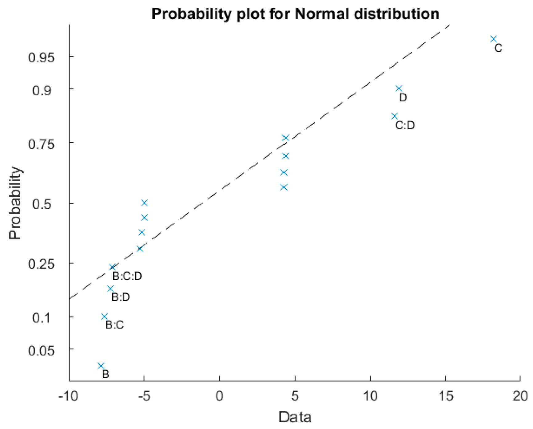
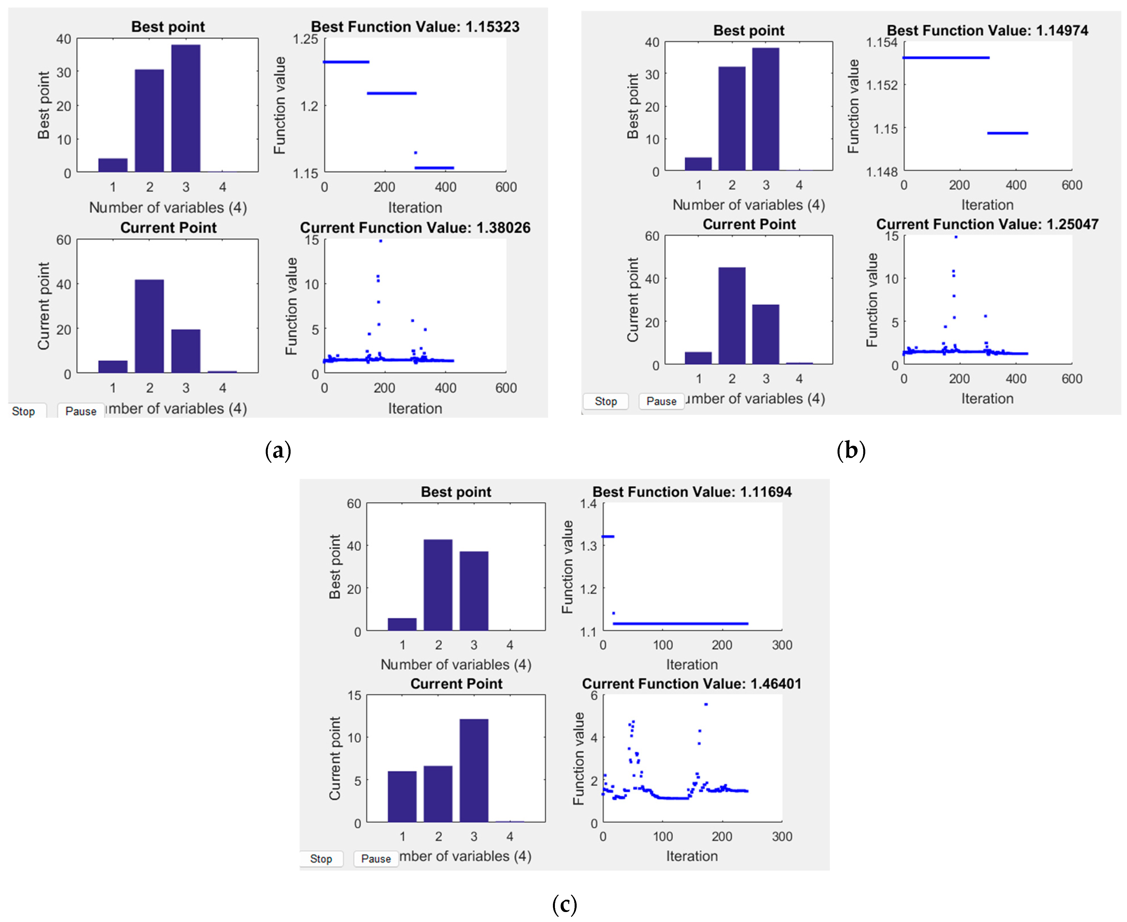
Several optimization methods were tested, beginning with statistical analyses, in particular, the design of experiments (DOE) and the response surface methodology, followed by parametric search (PS), the Monte Carlo method (MC), and simulated annealing (SA). It was also examined whether a full analysis was necessary or whether some preselection could be applied. Certain parts required computation in Maple due to the need for increased numerical precision, while other parts could be handled in MATLAB.

4. Particular Case Analysis

4.1. Preliminary Tests

In this section, a particular case is tested to check the viability of the PI definition given by Equation (16). Such cases must include a sufficiently large region of $in{d}_p$, where the difference between the PCV and ${\alpha }_{res}$ or ${\alpha }_{m50}$ is significant; otherwise, improvement is not feasible. For this selection, the analysis of the number of resonances is useful, because these cases must have a reduced number of resonances. The selected case is characterized by ${\mu }_s=3$, ${\mu }_b=10$, and ${\eta }_s=0$. Two indexes are chosen to characterize ${\kappa }_b$, namely $in{d}_b=20$ and $in{d}_b=63$. Moreover, $in{d}_p$ is tested for discrete values $in{d}_p=1:1:51$. The results are presented in Figure 12.

Several curves are plotted in Figure 12. In the legend, “peak” means $\alpha$ at the first peak in the upward displacement, identifying the lowest PCV determined using parametric analysis in MATLAB.

It can be concluded from Figure 12b that the PCV line is not realistic, because it should be smooth. A very accurate calculation is carried out by implementing function envelopes for the propagating part of the solution; thus, this decrease is not a numerical error, but an indication of a premature peak, which should be disregarded for PCV determination. Following regularization, the graph in Figure 13 is obtained.

From Figure 12 and Figure 13, it can be concluded that there is a sufficiently large region of $in{d}_p$, where the difference between the PCV and ${\alpha }_{res}$ or ${\alpha }_{m50}$ is quite large, confirming the feasibility of the adopted approach. Calculating the PI for these cases, values of 1.3854 at $in{d}_p=19$ and 0.5412 at $in{d}_p=18$ are obtained for $in{d}_b=20$ and $in{d}_b=63$, respectively.

However, it is not sufficient to calculate the PI alone, because the feasibility of the data used must be confirmed. First, Equations (12) and (15) must be fulfilled. Unfortunately, this is still not sufficient.

4.2. Real Data Identification

Even if Equations (12) and (15) confirm the feasibility of the dimensionless parameters, this does not guarantee the existence of a real data set within the intervals from Equation (11) and the specified ranges for $m_s$, $k_p$, ${\rho }_b$, and $E_b$, as indicated in Section 2 (text below Figure 2). It is also necessary to consider realistic values for $m$ ($m=54 \mathrm{kg}/\mathrm{m}$ or $m=60 \mathrm{kg}/\mathrm{m}$) and $k_f\in 〈0.22;1000〉 {\mathrm{MN}/\mathrm{m}}^2$, as in [18], which complete the full set of parameters, defining the intervals indicated in Equation (10).

The selection of real parameters can be conveniently carried out in the following way. First, the stress cone is parameterized according to:

$$l_s=0.5:0.1:0.8, h_b=0.2:0.05:0.6, l_b=0.2:0.02:0.36, {\alpha }_b={25}^{\mathrm{o}}:5^{\mathrm{o}}:{50}^{\mathrm{o}}$$

(17)

For each set of parameters, the dynamically activated ballast volume $m_{cn}$ is calculated in [m³], and the parameter related to the ballast layer’s vertical stiffness $k_{cn}$ is calculated in [m]. Knowing the optimal values, i.e., the target values ${\mu }_s$, ${\mu }_b$, ${\kappa }_p$, and ${\kappa }_b$, it must hold that:

$$\begin{gathered} {\displaystyle \frac{m_s^{-}}{{\rho }_b^{+}}}={\displaystyle \frac{40}{2600}}={\displaystyle \frac{1}{65}}\le \left(m_{cn}{\displaystyle \frac{{\mu }_s}{{\mu }_b}}={\displaystyle \frac{m_s}{{\rho }_b}}\right)\le {\displaystyle \frac{m_s^{+}}{{\rho }_b^{-}}}={\displaystyle \frac{160}{1200}}={\displaystyle \frac{1}{7.5}}, \\ {\displaystyle \frac{k_p^{-}}{E_b^{+}}}={\displaystyle \frac{20}{400}}=0.05\le \left(k_{cn}{\displaystyle \frac{{\kappa }_p}{{\kappa }_b}}={\displaystyle \frac{k_p}{E_b}}\right)\le {\displaystyle \frac{k_p^{+}}{E_b^{-}}}={\displaystyle \frac{5000}{50}}=100 \end{gathered}$$

(18)

Then, if these conditions are fulfilled, the selection can continue by defining the admissible values:

$$\begin{gathered} {\widehat{m}}_s^{-}=\max \left(m_s^{-},{\rho }_b^{-}{m}_{cn}{\displaystyle \frac{{\mu }_s}{{\mu }_b}}\right)=\max \left(40,1200m_{cn}{\displaystyle \frac{{\mu }_s}{{\mu }_b}}\right), \\ {\widehat{m}}_s^{+}=\min \left(m_s^{+},{\rho }_b^{+}{m}_{cn}{\displaystyle \frac{{\mu }_s}{{\mu }_b}}\right)=\min \left(160,2600m_{cn}{\displaystyle \frac{{\mu }_s}{{\mu }_b}}\right), \end{gathered}$$

(19)

$$\begin{gathered} {\widehat{k}}_p^{-}=\max \left(k_p^{-},E_b^{-}{k}_{cn}{\displaystyle \frac{{\kappa }_p}{{\kappa }_b}}\right)=\max \left(20,50k_{cn}{\displaystyle \frac{{\kappa }_p}{{\kappa }_b}}\right), \\ {\widehat{k}}_p^{+}=\min \left(k_p^{+},E_b^{+}{k}_{cn}{\displaystyle \frac{{\kappa }_p}{{\kappa }_b}}\right)=\min \left(5000,400k_{cn}{\displaystyle \frac{{\kappa }_p}{{\kappa }_b}}\right), \end{gathered}$$

(20)

Further:

$${\widehat{m}}^{-}={\displaystyle \frac{{\widehat{m}}_s^{-}}{l_s{\mu }_s}}, {\widehat{m}}^{+}={\displaystyle \frac{{\widehat{m}}_s^{+}}{l_s{\mu }_s}}, {\widehat{k}}_f^{-}={\displaystyle \frac{{\widehat{k}}_p^{-}}{l_s{\kappa }_p}}, {\widehat{k}}_f^{+}={\displaystyle \frac{{\widehat{k}}_p^{+}}{l_s{\kappa }_p}},$$

(21)

Finally, if the interval $〈{\widehat{m}}^{-},{\widehat{m}}^{+}〉$ has some intersection with $〈m^{-},m^{+}〉=〈54,60 〉\mathrm{kg}/\mathrm{m}$, and also the interval $〈{\widehat{k}}_f^{-},{\widehat{k}}_f^{+}〉$ has some intersection with $〈k_f^{-},k_f^{+}〉=〈0.22;1000〉 {\mathrm{MN}/\mathrm{m}}^2$, then feasible design values can be found. As only two rail profiles are commonly used, either 54 or 60 kg/m is selected. For each of these profiles, $EI$ is known. It was further confirmed during the use of other optimization techniques that the optimal $k_f$ is usually very high; thus, during this procedure, it is more convenient to use the lowest feasible value. This completes the definition of the reference beam, and the missing values are simply calculated.

All the results are summarized in the tables, which are conveniently placed in Appendix A, so that the results of all the methods can be consulted together. In

Table A1. Summary of the best solutions obtained for each method.

Type	${\mathbf{\mu }}_{\mathbf{s}}$	${\mathbf{\mu }}_{\mathbf{b}}$	$\mathbf{i}\mathbf{n}{\mathbf{d}}_{\mathbf{p}}$	$\mathbf{i}\mathbf{n}{\mathbf{d}}_{\mathbf{b}}$	${\mathbf{\eta }}_{\mathbf{s}}$	PI	PCV	${\mathbf{\alpha }}_{\mathbf{r}\mathbf{e}\mathbf{s}}$	%
DOE	4	12	16	40	0	0.4956	0.4456	0.6419	44.05
$\mathrm{MC} \left(d{a}_{0.01}^{\%}\right)$	5.5244	44.1292	20	44.8870	0.1111	0.7163	0.2326	0.7112	205.76
$\mathrm{PS}1 \left(d{a}_{0.01}^{\%}\right)$	1	16	17	49	0	0.4410	0.4257	0.6624	55.60
$\mathrm{PS}2 \left(d{r}^{\%}\right)$	1	16	18	50	0	0.4505	0.4115	0.6816	65.64
$\mathrm{PS}3 \left(d{a}_{0.01}^{\%}\right)$	3.5	42	13	40	0	0.2159	0.2517	0.5845	132.22
$\mathrm{PS}4 \left(d{r}^{\%}\right)$	3.5	42	19	46	0	0.3355	0.2462	0.6945	182.10
$\mathrm{SA} \left(d{a}_{0.01}^{\%}\right)$	5.3333	42.8571	12	47.3333	0	0.2055	0.2437	0.5660	132.22

, the main optimized data are given in the form of optimized dimensionless parameters, PI, PCV, and an indication of a possible extension, both through the use of the absolute $\alpha$-value and the percentage increase with respect to the PCV.

Table A2. Summary of the feasible data of the stress cone obtained for each method.

Type	${\mathbf{l}}_{\mathbf{s}}$ [m]	${\mathbf{h}}_{\mathbf{b}}$ [m]	${\mathbf{\alpha }}_{\mathbf{b}}$ [°]	${\mathbf{l}}_{\mathbf{b}}$ [m]	${\mathbf{m}}_{\mathbf{c}\mathbf{n}}$ [m3]	${\mathbf{k}}_{\mathbf{c}\mathbf{n}}$ [m]
DOE	0.6	0.3	50	0.36	0.2231	2.3821
DOE	0.6	0.35	25	0.2	0.1510	1.089
$\mathrm{MC} \left(d{a}_{0.01}^{\%}\right)$	0.5	0.6	50	0.34	0.4592	1.2568
$\mathrm{PS}1 \left(d{a}_{0.01}^{\%}\right)$	0.8	0.3	50	0.36	0.2682	2.6634
$\mathrm{PS}2 \left(d{r}^{\%}\right)$	0.8	0.3	50	0.36	0.2682	2.6634
$\mathrm{PS}3 \left(d{a}_{0.01}^{\%}\right)$	0.7	0.6	50	0.3	0.6128	1.5289
$\mathrm{PS}4 \left(d{r}^{\%}\right)$	0.7	0.6	50	0.3	0.6128	1.5289
$\mathrm{SA} \left(d{a}_{0.01}^{\%}\right)$	0.5	0.6	50	0.32	0.4577	1.2442

summarizes the parameters of the stress cone;

Table A3. Summary of the other data to match the optimized parameters ($v_{res}$ indicates the velocity at a given resonance).

Type	$\mathbf{m}$ [kg/m]	${\mathbf{m}}_{\mathbf{s}}$ [kg]	${\mathbf{\rho }}_{\mathbf{b}}$ [kg/m3]	${\mathbf{k}}_{\mathbf{f}}$ [MN/m2]	${\mathbf{k}}_{\mathbf{p}}$ [MN/m]	${\mathbf{E}}_{\mathbf{b}}$ [MPa]	DCV [m/s]	${\mathbf{v}}_{\mathbf{r}\mathbf{e}\mathbf{s}}$ [m/s]
DOE	60	144	1937	198	20	177	449	646
DOE	54	130	2575	198	20	388	473	681
$\mathrm{MC} \left(d{a}_{0.01}^{\%}\right)$	54	149	2594	150	20	372	230	704
$\mathrm{PS}1 \left(d{a}_{0.01}^{\%}\right)$	54	43.2	2577	132	20	399	408	636
$\mathrm{PS}2 \left(d{r}^{\%}\right)$	54	43.2	2577	118	20	399	384	636
$\mathrm{PS}3 \left(d{a}_{0.01}^{\%}\right)$	54	132.3	2591	239	20	390	280	651
$\mathrm{PS}4 \left(d{r}^{\%}\right)$	54	132.3	2591	120	20	390	231	651
$\mathrm{SA} \left(d{a}_{0.01}^{\%}\right)$	54	144	2528	376	20	396	304	705

lists the other values used to match the optimized data.

4.3. Design of Experiments and Response Surface

The DOE and the response surface were the first optimization approaches used. Unfortunately, the response surface did not yield any improvements. When a larger design domain was used, several cases with a set of fixed parameters ${\mu }_s$, ${\mu }_b$, $in{d}_b$, and ${\eta }_s$ produced an undefined PI, because no improvements were possible across the full range of the $in{d}_p$. Consequently, it was necessary to use a penalizing value, which distorted the response surface. Even based on a more restricted design domain encompassing the particular case detailed in Section 4.1, a reasonable estimate of the already known values was never obtained. A Monte Carlo search within the response surface indicated that the best choice is located one of the factorial design points. The residues were not well-behaved and, thus, this type of analysis had to be disregarded in further steps.

After excluding non-feasible cases, the best result from this analysis was PI = 0.4956, corresponding to the parameter set: ${\mu }_s=4$, ${\mu }_b=12$, $in{d}_b=40$, ${\eta }_s=0$, and $in{d}_p=16$. In this case, the full factorial design was performed for ${\mu }_s^{-}=2$, ${\mu }_s^{+}=4$, ${\mu }_b^{-}=8$, ${\mu }_b^{+}=12$, $in{d}_b^{-}=40$, $in{d}_b^{+}=80$, ${\eta }_s^{-}=0$, and ${\eta }_s^{+}=1$, and the best feasible choice corresponded to the combination ++−−. The results of this analysis are presented in Figure 14, which shows that PCV = DCV can be increased by 44.05%. The numerical values are included in Table A1.

In Figure 14, the yellow dashed line marks the first peak in the upward displacement, identifying this way the PCV = DCV. The second criterium is governed by ${\alpha }_{res}$, which is not marked by a vertical line because it is identified through the properties of the CV, that is, a sudden jump to zero displacement at the AP. The corresponding probability plot is shown in Figure 15.

The best design obtained during the DOE (line 1 in Table A1) offers many possibilities for selecting a corresponding set of real data. As it is not feasible to present all of them, only two representative cases are selected, and the corresponding values are provided in Table A2 and Table A3.

5. Optimization and Parametric Search

Because a full analysis (as shown in Figure 12 and Figure 13 and performed during the DOE) is time consuming, it is not suitable to implement it in metaheuristic methods or parametric search. Consequently, these methods were only applied to certain preselected favorable cases, after which the best case was further analyzed over values of $in{d}_p$. Preselection was implemented in two ways: based on cases with the highest differences in ${\alpha }_{as}^{0.01}$ or in ${\alpha }_{res}$ over the range of $in{d}_p$. Moreover, ${\alpha }_{as}^{0.01}$ can be easily extracted in MATLAB; however, lower damping levels are prone to numerical errors, due to MATLAB’s double precision. Thus, ${\alpha }_{res}$ had to be calculated in Maple because high precision in regard to the root determination is required. In what follows, $d{a}_{0.01}^{\%}$ will be used for the percentage difference in ${\alpha }_{as}^{0.01}$ over the range of $in{d}_p$ and $d{r}^{\%}$ will be used for the percentage difference in ${\alpha }_{res}$.

5.1. Monte Carlo Method

The MC method was used to prelect the most favorable cases according to the $d{a}_{0.01}^{\%}$. The design domain was defined as ${\mu }_s^{-}=1$, ${\mu }_s^{+}=6$, ${\mu }_b^{-}=2$, ${\mu }_b^{+}=45$, $in{d}_b^{-}=1$, $in{d}_b^{+}=101$, ${\eta }_s^{-}=0$, and ${\eta }_s^{+}=1$.

It was not useful to repeat the analysis, because the MATLAB function rand tends to reuse the same randomization, and several tested cases were duplicated. The best value obtained was 88.89%, achieved for ${\mu }_s=5.5244$, ${\mu }_b=44.1292$, $in{d}_b=44.8870$, and ${\eta }_s=0.1111$. This case was then analyzed in regard to the PI. The results of the analysis over values of $in{d}_p$ are presented in Figure 16. The asymptote and instability were only tested in the relevant region where the PCV does not coincide with the ${\alpha }_{res}$.

After that, the minimum value of the PI was identified and the corresponding $in{d}_p$ was gradually increased until at least one feasible design data set appeared. This happened for $in{d}_p=11$, where PI = 0.1905. The numerical data obtained are summarized in Table A1, Table A2 and Table A3. The final results are shown in Figure 17. Moreover, ${\alpha }_{res}$ is again decisive for the PI, and the possible increase in the DCV is 205.76%.

5.2. Parametric Search

PS was also performed using the preselected most favorable cases. Both $d{a}_{0.01}^{\%}$- and $d{r}^{\%}$-based options were used. The results of the preselected cases are shown in Figure 18 and Figure 19.

After preselection, the four best cases were analyzed in regard to the PI over the $in{d}_p$. Moreover, the $in{d}_p$ at the minimum PI was gradually increased until at least one feasible design appeared. The final results are shown in Figure 20, Figure 21, Figure 22 and Figure 23. The ${\alpha }_{res}$ is again decisive for the PI.

The PI values in these four cases are 0.4257, 0.4115, 0.2517, and 0.2462, leading to a possible increase in the DCV of 55.60%, 65.64%, 132.22%, and 182.10%, respectively. The numerical data are summarized in Table A1, Table A2 and Table A3.

5.3. Simulated Annealing

SA was selected as another metaheuristic optimization method, due to its ease of implementation in MATLAB. The predefined parameters governing the optimization process were kept unchanged. The design domain was defined as ${\mu }_s^{-}=1$, ${\mu }_s^{+}=6$, ${\mu }_b^{-}=2$, ${\mu }_b^{+}=45$, $in{d}_b^{-}=1$, $in{d}_b^{+}=50$, ${\eta }_s^{-}=0$, and ${\eta }_s^{+}=2$, and used in this order. Several initial data sets were used for the preselection according to $1/d{a}_{0.01}^{\%}$, in order to search for a minimum.

Figure 24 shows the results of the different runs.

The best value obtained is 1.46401, corresponding to 89.53%, which is better than that obtained by the MC method (88.89%), but worse than that from the PS (89.90%). The preselected parameters, ${\mu }_s=5.3333$, ${\mu }_b=42.8571$, $in{d}_b=37.3333$, and ${\eta }_s=0$, were then used for detailed analysis of the PI. As before, $in{d}_p$ at the minimum value of the PI was gradually increased until at least one feasible design appeared, which occurred for $in{d}_p=12$, for which PI = 0.2055. The results of the analysis over the $in{d}_p$ range are presented in Figure 25. The asymptote and instability were again tested only in the relevant region where the PCV does not coincide with the ${\alpha }_{res}$.

The final results are shown in Figure 26. Moreover, ${\alpha }_{res}$ is again decisive. DCV = 0.2437 could allow for an additional increase of 132.22%.

6. Discussion

In the previous sections, several feasible designs for which the PI was evaluated as optimal have been presented. It is worthwhile to remark that ${\alpha }_{m50}$ was never decisive in these cases, and the extension of the DCV was always guided by the ${\alpha }_{res}$. From Table A1, it is evident that ${\mu }_s$ and ${\mu }_b$ exhibit higher dispersion, while $in{d}_p$ and $in{d}_b$ have very similar values in all cases. Finally, ${\eta }_s=0$ appears almost exclusively, except in results of the MC method, likely because a zero value was unlikely to be selected randomly, along with other optimal parameters. Furthermore, a higher ${\mu }_s$ generally provides larger improvements, and $in{d}_p$ is always much lower than $in{d}_b$.

Moreover, $in{d}_p$ at a minimum value of the PI was gradually increased until at least one feasible design appeared in all cases, except for the DOE, where, in fact, no optimization was presented. Since these designs are the first to appear, this implies that some data will lie at the limit values in the considered ranges. As such, they might seem unrealistic, but it must be noted that a further increase in the $in{d}_p$ can lead to better selections, without significantly compromising the PI value. Generally, for a higher $in{d}_p$, the possible increase up to ${\alpha }_{res}$ is more favorable; however, in this scenario, the ratio $\left|{\tilde{w}}_{\min }^{PCV}\right|/{\tilde{w}}_{st}$ increases.

Parametric searches with a base value of ${\mu }_s=1$ can naturally only identify designs where the attainment of this is possible, meaning designs using wooden sleepers. Nevertheless, this option was not disregarded, because it is essential to consider the possibility of using novel lightweight materials in the future.

Some of the real data presented in Table A2 and Table A3 may seem unreasonable, but that is a consequence of how the initial ranges for all values were chosen.

Due to the consistency of the results obtained using different approaches, exploring other methods would not be useful.

The results confirm that preselection is useful and reduces the calculation time, but the connections are not straightforward. It is not necessarily true that the best preselection yields the best PI and, at the same time, the highest possible increase in the DCV.

When using the lowest feasible $in{d}_p$, combinations with a relatively high $in{d}_b$ led to the appearance of the lowest $k_p$ found in the literature in regard to all the feasible data shown in Table A3. Similarly, for the same reason, $k_f$ is relatively high, resulting in quite a high DCV, which is difficult to achieve with current train designs. This implies that although the possible increase is large, it may not be practically important. Nevertheless, these results may inspire the adoption of new approaches and provide guidance toward optimizing track design.

Further analyses are needed to verify whether the PI was defined appropriately or if it should be modified. Since instability was never found to be decisive, it can likely be excluded from this analysis, enabling more detailed investigations of other aspects.

Additional tests are also necessary, because although several authors use this model without considering shear resistance, it must be verified whether such modeling is truly valid considering practical applications.

7. Conclusions

In this paper, the tailoring of input geometric and material data of railway tracks were presented, with the objective of identifying cases where the first increase in vibrations is negligible and can, therefore, be bypassed.

Several optimization techniques and approaches were employed, leading to similar conclusions. However, the results require further examination in regard to several aspects. In particular, the adequacy of the proposed PI must be evaluated. Since all the results showed a very high DCV with a negligible increase in vibrations, the significance of a further increase diminishes. It is, thus, necessary to investigate whether similar outcomes could be achieved for lower real-world velocities, where the potential for meaningful improvements is greater.

The results were obtained semi-analytically, with very high precision. This was crucial for accurately determining the number of resonances and identifying the first peak in the upward vibration.

It was found that the DCV can be significantly increased by optimizing the design parameters. However, such cases almost exclusively result in designs where the DCV is already very high. Therefore, the practical significance of a further increase becomes questionable, as already mentioned above.

In all cases, very soft rail pads emerged in the final optimized design. It is essential to verify whether such configurations are feasible. Thus, the results suggest a tendency toward the following:

• Very high foundation stiffness;
• Low rail pad stiffness;
• Zero ballast shear stiffness.

In particular, further research is needed regarding ballast shear stiffness. In actual designs, eliminating it entirely may not be realistic. While it might be reduced via rail pretension, such an approach is not practical.

Due to the scope of this study, these aspects will be addressed in future research. It is believed that the theoretical findings presented here can contribute to the development of optimal track designs, incorporating novel materials. Their implementation in real-world designs remains a subject for further investigation.

Finally, it is important to note that point load idealization can lead to a singularity in displacement at the critical velocity. A more realistic distributed load over a finite contact area, even if it is short, will still result in elevated vibrations near those velocities, but the dynamic response will be smoother and the displacements will remain finite. Thus, singularity at the critical velocity is eliminated. This fact complicates the analysis in the present paper, as the identification of a true resonance was essential. Nevertheless, while such an adjustment would influence the amplitude and sharpness of the vibration peaks, it does not fundamentally alter the existence or location of the PCVs. Therefore, I expect the general trends observed during the optimization process and the qualitative behavior of the system to remain valid under more realistic loading conditions. Incorporating distributed or smoothed load profiles will be considered in future work to further assess their influence on resonance characteristics and design robustness.