Cross-Floor Vibration Wave Propagation in High-Rise Industrial Buildings Under TMD Control

Abstract

High-rise industrial buildings are particularly susceptible to vibration-induced comfort issues, which can negatively impact both the health and productivity of workers and office staff. Unlike most existing studies that focus on local structural components, this study proposes and validates a wave propagation analysis (WPA) method to predict peak accelerations of the floor caused by excitations located on different floors. The method is validated through on-site vibration tests conducted on a high-rise industrial building with shared factory and office space. A simplified regression-based propagation equation is further developed to facilitate practical design applications. The regression parameters are fitted using theoretical calculation results, enabling rapid prediction of peak acceleration responses on the same or different floors. To enhance vibration control, tuned mass dampers (TMDs) are installed on selected floors, and additional tests are conducted with the TMDs activated. An insertion loss-based correction is introduced into the WPA framework to account for the TMD’s frequency-dependent attenuation effects. The extended method supports both accurate prediction of vibration reduction and optimisation of TMD placement across multiple floors in high-rise industrial buildings.

1. Introduction

High-rise buildings are essential infrastructure in modern urbanisation, enabling cities to accommodate larger populations, and industrial facilities. A key innovation in these structures is the high-rise multifunctional design, which combines office spaces, research areas, and industrial production within a single building. This concept allows for a functional separation, with research activities on the lower floors and production facilities on the upper floors. However, vibration waves generated by equipment on the middle or upper floors can spread throughout the entire building, potentially leading to health problems for workers in both office and production areas. An example of such a building is the Pingshan Biopharmaceutical Industrial Building, depicted in Figure 1. This structure is constructed with concrete-filled steel tubular columns, steel beams, and reinforced truss floor slabs, standing 83.75 m tall with 12 floors.

In current design practices, the propagation of vibration waves caused by equipment is often not a primary consideration, particularly in tall, mixed-use buildings. Moreover, there is a shortage of theoretical or computational methods that can reliably predict how vibration waves spread in multi-story steel–concrete composite structures. With the inevitable rise in the construction of high-rise industrial buildings over the next decade, there is an urgent need for systematic research into this emerging issue. The absence of effective design tools for predicting and managing structural vibrations in modern multifunctional industrial buildings must be addressed.

Modern high-rise steel–concrete composite industrial buildings, often surpassing ten stories and reaching heights of over 30 m, with some even approaching 100 m, differ significantly from traditional multi-story industrial structures. In many of these buildings, large industrial machinery is placed in the middle or upper floors, which shifts the building’s centre of gravity and exacerbates vibration problems [1]. These factors make vibrations caused by equipment a major issue, underscoring the need for more precise theoretical models and effective design strategies to control vibrations in such buildings.

Numerous studies have focused on vibration challenges in traditional low-rise and multi-story industrial buildings. Gasella [2] performed numerical simulations on individual structural components to assess the effects of equipment-induced translational and torsional vibrations, identifying the locations of peak responses. Li and Peng [3] conducted on-site dynamic testing and computer simulations on individual components to examine resonance effects when the natural frequencies of the structure approach the excitation frequency of the equipment. Carlson and Spencer [4] utilised perturbation methods to explore the influence of equipment vibrations on low-stiffness, small-damping structural components. Lung [5] introduced a modified response spectrum calculation approach for individual components in scenarios where the frequencies of the equipment and structure are closely matched.

Tuned mass dampers (TMDs) have been widely recognised as effective tools for mitigating vibrations in high-rise buildings. In a study by Salah et al. [6], the performance of multiple TMDs was analysed, demonstrating significant reductions in vibration responses when placed strategically in multi-story buildings under seismic excitations. Similarly, a study by Hamid et al. [7] explored the optimal placement of distributed TMDs in tall buildings, highlighting that carefully positioning these dampers can enhance vibration control during both seismic and wind-induced excitations. Additionally, Tsiavos et al. [8] presented a low-cost and sustainable timber-based tuned mass damper system that can be installed in existing floor slabs for the response modification of the dynamic behaviour of buildings. These studies underline the importance of TMD optimisation for effective vibration reduction in high-rise industrial buildings.

Two cutting-edge TMD variants have also attracted considerable attention. The Tuned Mass Damper Inerter (TMDI) augments the classical TMD with an inerter element, markedly boosting control efficiency at low mass ratios; recent studies have optimised its parameters and validated its performance in high-rise buildings and base-isolated systems [9,10,11]. Meanwhile, the Negative-Stiffness TMD (NS-TMD) and its hybrids (e.g., TNIMD, TMNSDI) introduce equivalent negative stiffness—via buckled struts, magneto-elastic devices, or frictional sliders—to widen the effective frequency band and suppress peak responses [12,13,14,15,16]. Comparative analysis indicates that TMDIs excel when the mass budget is limited, whereas NS-TMDs better handle multi-modal or broadband excitations; both can be seamlessly integrated into the TMD-WPA framework proposed herein to furnish more adaptable vibration control strategies for industrial high-rise structures.

Various methods have been utilised in vibration wave propagation research, including the transfer function method, transfer matrix method, impedance synthesis method, admittance method, spectral analysis method, and the wave propagation analysis (WPA) method. Among these, the WPA method stands out for its ability to manage boundary and constraint conditions effectively while maintaining clarity in its mathematical formulation. Wu and Mead [17] initially applied the WPA method to bending waves in multi-support Bernoulli–Euler beams, and Tso and Hansen [18] extended it to analyse wave transmission in plates and cylinders. Later, Qin and Zeng [19], Chen and Zhang [20], and Zhou et al. [21] adapted the WPA method to study more complex structural systems. Despite these developments, the majority of WPA applications remain focused on individual structural components like slabs or columns, with few studies exploring the propagation of vibration waves across entire high-rise buildings [22].

This study expands the WPA method to examine vibration wave propagation in a high-rise steel–concrete composite industrial building. The analysis considers vibration wave transmission within beams, columns, and slabs on the same floor, as well as across floors through slab–column connections. A novel calculation method and regression equations for vibration wave propagation are introduced, and these are validated using on-site test data from the building (Figure 1). The proposed approach allows for the theoretical prediction of structural responses at any location within the building, based on vibration excitations from any other point within the same structure.

2. The Calculation Theory of the WPA Method

2.1. Forced Vibration of a Rectangular Plate Structure with Simply Supported on All Four Edges

Consider a simply supported rectangular plate, that is a typical model of a concrete floor slab. The four edges of the slab are defined by $x=0$, $x=L_x$, $y=0$, and $y=L_y$, respectively. It is assumed that the following pressure wave load ${\tilde{P}}_0(x,y,t)$ acts on the surface of the plate [17], which is

$${\tilde{P}}_0(x,y,t)=P_0{e}^{j(\omega t-k_{p}x)},$$

(1)

where $P_0$ is the amplitude of a pressure wave; $\omega$ is the circular frequency of the pressure wave; $k_p$ is the wave number in the $x$-direction of the pressure wave; and $t$ denotes time. We nevertheless acknowledge that a broadband or time-varying load would require a spectral input model, and, in that case, the analytical framework presented here would need to be extended to account for multiple frequencies.

Equation (1) represents the propagation of a vibrational pressure wave along the $x$-direction, with a propagation speed, $v_p$, of

$$v_p=\omega /k_p.$$

(2)

At a given time $t$ and location $x$, $p$ represents the sinusoidal component in the $y$-direction. Thus

$${\tilde{P}}_0(x,y,t)={\displaystyle \sum _{r=1}^{\infty }{p}_r\frac{\sin (2r-1)\pi y}{L_y}}={\displaystyle \sum _{r=1}^{\infty }{p}_r\sin (k_{ry}y)},$$

(3)

where $k_{ry}=m\pi /L_y$ represents the wave number in the $y$-direction.

We consider the case when the half-wave length of the pressure is equal to the length of the plate in the $y$-direction. Thus,

$${\tilde{P}}_0(x,y,t)=p_1\sin (k_{1y}y)e^{j(\omega t-k_{p}x)}.$$

(4)

The displacement of the plate, $w_p(x,y,t)$, satisfies the following equation:

$$D{\nabla }^4{w}_p(x,y,t)+\rho h{\omega }^2{w}_p(x,y,t)=p_1\sin (k_{1y}y)e^{j(\omega t-k_{p}x)},$$

(5)

where $D$ is the bending stiffness of the plate; $\rho$ is the density of the plate; and $h$ is the thickness of the plate. By assigning a complex bending stiffness $D(1+j\tau )$, the internal damping of the plate can be considered, where $\tau$ is the damping loss factor.

The solution of Equation (5) consists of two parts: the particular solution and the complementary solution. The particular solution $w_1$ represents the response of an infinitely long plate in the $x$-direction, describing the propagation of pressure waves in the $x$-direction. The complementary solution $w_2$ represents the response of a finite-length plate. The waves will be reflected when they propagate and encounter the plate boundaries, and the structural wave reflected from all boundaries will generate the far-field wave and near-field wave.

Therefore, the total displacement $w_p(x,y,t)$ can be expressed as

$$\begin{array}{l}{w}_p(x,y,t)=w_1+w_2\\ =\left[A_1{e}^{k_{n}x}+A_2{e}^{-k_{n}x}+A_3{e}^{j{k}_{x}x}+A_4{e}^{-j{k}_{x}x}+{\displaystyle \frac{p_1{e}^{-j{k}_{p}x}}{D(k_{1y}^2+k_p^2)-ph{\omega }^2}}\right]\sin (k_{1y}y)e^{j\omega t}\end{array}.$$

(6)

where $k_n^2=k^2+k_{1y}^2$, $k_x^2=k^2-k_{1y}^2$, and $A_n$ is an unknown coefficient.

The solution includes four unknowns, which can be determined by satisfying the four boundary conditions. For the case of simply supported edges, the boundary conditions are

$$\left.\begin{array}{l}w=0\\ {\displaystyle \frac{{\partial }^{2}w}{\partial x^2}}=0\end{array}\right\}$$

(7)

at $x=0$ and $x=L_x$, and

$$\left.\begin{array}{l}w=0\\ {\displaystyle \frac{{\partial }^{2}w}{\partial y^2}}=0\end{array}\right\}$$

(8)

at $y=0$ and $y=L_y$.

The four unknown constants, $A_n$ ($n=$ 1, 2, 3, and 4), can be obtained by solving Equation (9):

$$\begin{array}{l}\left[\begin{array}{cccc}1& 1& 1& 1\\ k_n& -k_n& j{k}_x& -j{k}_x\\ e^{k_n{L}_x}& e^{-k_n{L}_x}& e^{j{k}_x{L}_x}& e^{-j{k}_x{L}_x}\\ k_n{e}^{k_n{L}_x}& -k_n{e}^{-k_n{L}_x}& j{k}_x{e}^{j{k}_x{L}_x}& -j{k}_x{e}^{-j{k}_x{L}_x}\end{array}\right]\left\{\begin{array}{l}{A}_1\\ A_2\\ A_3\\ A_4\end{array}\right\}\\ =\left\{\begin{array}{c}1\\ -j{k}_p\\ e^{-j{k}_p{L}_x}\\ -j{k}_p{e}^{-j{k}_p{L}_x}\end{array}\right\}{\displaystyle \frac{p_1}{D(k_{1y}^2+k_p^2)-\rho h{\omega }^2}}\end{array}.$$

(9)

Therefore, for given $k_p$ and $\omega$, the displacement at any point on the plate can be expressed as

$$w_p(x,y,t)=Y(x,y,k_p,\omega )p_1{e}^{j\omega t}$$

(10)

where $Y(x,y,k_p,\omega )$ represents the wave response function.

By taking the first and second derivatives of Equation (10) with respect to $t$, the velocity and acceleration of the plate can be obtained.

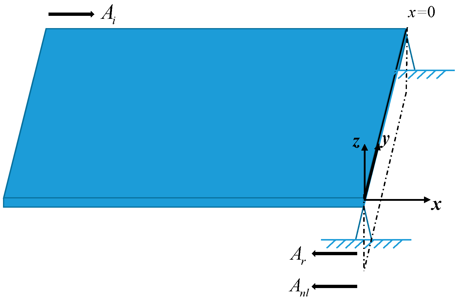
2.2. Wave Propagation at the Vertical Incidence of Bending Wave in Boundary Interface

Part or all of the waves travelling through a structure will reflect during propagation when meeting discontinuities and generate near-field waves on the reflecting interface.

Assume that the uniform plate structure shown in Figure 2 is discontinuous at $x=0$. The incident pressure wave ${\tilde{A}}_i$ in the region where $x<0$ is

$${\tilde{A}}_i=A_i{e}^{j(\omega t-kx)},$$

(11)

where $A_i$ represents the amplitude of the pressure wave; $\omega$ is the circular frequency of the pressure wave; and $k$ is the wave number of the pressure wave.

Structural wave reflection and transmission occur at $x=0$. The reflected wave can be expressed as

$${\tilde{A}}_r=A_r{e}^{j(\omega t+kx)},$$

(12)

where $A_r$ represents the amplitude of the reflected wave.

The near-field wave generated from the reflection interface is

$${\tilde{A}}_{nl}=A_{nl}{e}^{j(\omega t+kx)},$$

(13)

where $A_{nl}$ represents the amplitude of the reflected near-field wave.

Therefore, the displacements, $w_{p-}$, of the plate on the left-hand sides of the discontinuity can be described as

$$w_{p-}=(A_i{e}^{-jkx}+A_r{e}^{jkx}+A_{nl}{e}^{kx})e^{j\omega t}(x<0).$$

(14)

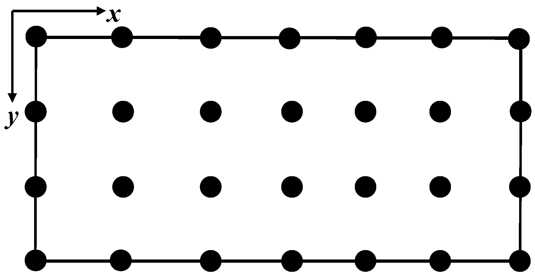
Based on the solutions in Section 2.1, a MATLAB R2021a code is formulated to calculate the propagation of vibration waves across a single floor. The boundary conditions along the outside beams are treated as simply supported edges (marked green in Figure 3).

Consider wave propagation in a plate with a simply supported edge at the end, as shown in Figure 2, where both displacement $w_p(0)$ and bending moment $M_{+}(0)$ and $M_{-}(0)$ must be zero, i.e.,

$$\left.\begin{array}{l}{w}_p(0)=0\\ M_{+}(0)=M_{-}(0)=0\end{array}\right\}.$$

(15)

Substituting Equation (14) into Equation (15), two reflected wave amplitudes, $A_r$ and $A_{nl}$, can be obtained, which are as follows:

$$\left.\begin{array}{l}{A}_r=-A_i\\ A_{nl}=0\end{array}\right\}.$$

(16)

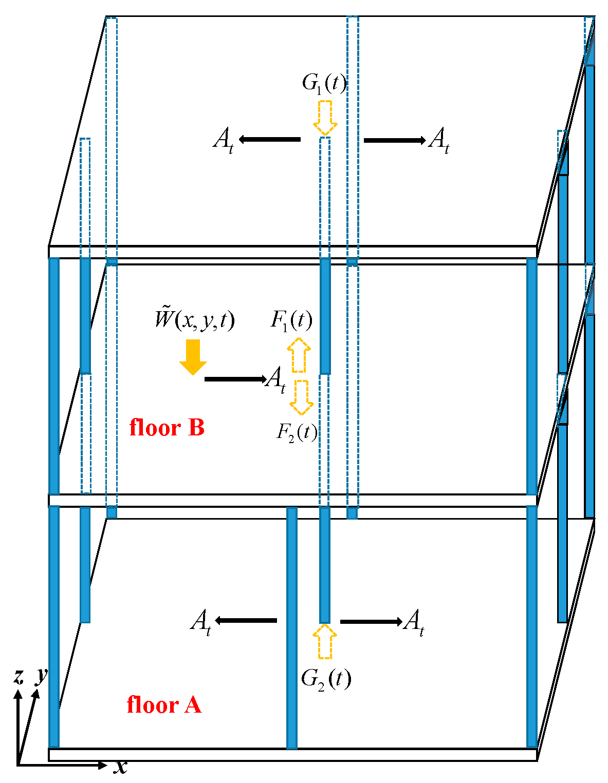
2.3. Calculation of Vibration Wave Propagation via Insertion Loss-Based Correction Under TMD Control

As described above, vibrational waves are generated under external load and then propagate across the floor. For slab–column connection, the resultant force $F_1(t)$ at the column base is obtained by integrating the normal stress distribution in the floor slab as follows:

$$F_1(t)={\displaystyle \underset{S}{\int }\sigma (x,y,t)dS={\displaystyle \underset{S}{\int }E\frac{\partial w_p(x,y,t)}{\partial y}}}dS,$$

(17)

where $\sigma (x,y,t)$ is the contact stress between the column end and the floor slab; $S$ is the cross sectional area of the column; $E$ is the Young’s modulus of the floor slab; and $w_p(x,y,t)$ is the displacement of the floor slab in the slab–column contact area.

Assuming that floor B is the source of vibration, Figure 4 schematically illustrates how the force is transmitted from floor B to floor A through a slab–column connections, where $F_1(t)$ and $F_2(t)$ represent, respectively, the axial force (load) acting at the bottom end of the column of floor B and the top end of the column of floor A. Equation (17) can be used to calculate the resultant force, $F_1(t)$, at the bottom end slab–column connection of floor B. The force is simultaneously transmitted to the top end of the column of floor A, which is denoted by $F_2(t)$.

Considering the relatively low stiffness of the slabs in comparison to the axial stiffness of the columns, the force in the column of floor B is considered to be fully transmitted to the column of floor A, i.e., $F_1(t)=F_2(t)$.

The forces, $F_1(t)$ and $F_2(t)$, propagate along their respect column axis in the opposite direction. The transmitted force of $F_1(t)$ at the top end of the column of floor B is denoted by $G_1(t)$, and transmitted force of $F_2(t)$ at the bottom end of the column of floor A is denoted by $G_2(t)$.

The propagation of the longitudinal waves in the columns satisfy

$${\displaystyle \frac{{\partial }^2{w}_c(z,t)}{\partial z^2}}={\displaystyle \frac{1}{{c_L}^2}}{\displaystyle \frac{{\partial }^2{w}_c(z,t)}{\partial t^2}},$$

(18)

where $c_L=\sqrt{E/\rho }$ represents the propagation speed of longitudinal waves. The free vibration wave, $w_c(z,t)$, expressed using a complex exponential form, is

$$w_c(z,t)=A{e}^{j\omega t-jkz}+B{e}^{j\omega t+jkz}=(A{e}^{-jkz}+B{e}^{jkz})e^{j\omega t},$$

(19)

where $A$ and $B$ are unknown coefficients; $k$ is the wave number of the pressure wave; and $\omega$ is the circular frequency of the pressure wave.

Due to the time delay in force transmission within the column, the solution of Equation (18) can be expressed as a single-variable function

$$w_c(z,t)=f(\xi ),$$

(20)

where $\xi =t-z/c_L$.

By substituting Equation (20) into Equation (18), the following equation is obtained

$${\displaystyle \frac{d^{2}f}{d{\xi }^2}}={\displaystyle \frac{1}{c_L^2}}·c_L^2{\displaystyle \frac{d^{2}f}{d{\xi }^2}}={\displaystyle \frac{d^{2}f}{d{\xi }^2}}.$$

(21)

Clearly, the equation satisfies the consistency condition. Therefore, the solution of Equation (18) can be any function propagating along the $t-z/c_L$.

Since the one-dimensional wave equation is a second-order partial differential equation, its general solution should include two independent solutions. Assuming the solution is the sum of two independent functions, it is represented as follows:

$$w_c(z,t)=f_1(t-z/c_L)+f_2(t+z/c_L),$$

(22)

where $f_1(t-z/c_L)$ represents the upward-propagating wave in the column of floor B; and $f_1(t+z/c_L)$ represents the downward-propagating wave in the column of floor A.

Therefore, an upward-propagating wave is generated when the external force $F_1(t)$ is applied at the bottom end of the column, which is

$$w_c(z,t)=f_1(t-z/c_L).$$

(23)

The wave reaches the top of the column when $t=L/c_L$ at $z=L$.

The stress and velocity of the column satisfy the following relationship:

$$\sigma =Z_{column}{\dot{w}}_c,$$

(24)

where $Z_{column}=\rho c_{L}S$ represents the wave impedance of the column; and ${\dot{w}}_c=\partial w_c/\partial t$ denotes the velocity of a particle within the column.

At the bottom end of the column of floor B, i.e., at $z=0$, the relationship between the resultant force and velocity is given by

$$F_1(t)=Z_{column}{\dot{w}}_c(0,t),$$

(25)

where

$${\dot{w}}_c(z,t)={\displaystyle \frac{\partial }{\partial t}}{f}_1(t-z/c_L).$$

(26)

Thus, the velocity at the top end of the floor B column is the time-delayed form of the velocity at the bottom end of the column.

Due to the effect of damping in the column, the resultant force at the top of the column on floor B, $G_1(t)$, is given by

$$G_1(t)=Z_{column}{\dot{w}}_c(L,t)e^{-\eta L}=Z_{column}{\dot{w}}_c(0,t-L/c_L)e^{-\eta L}=F_1(t-L/c_L)e^{-\eta L},$$

(27)

where $\eta ={\displaystyle \frac{\omega }{2\pi f}}\tan (\delta )$, and $\delta$ is the damping loss factor.

Similarly, the resultant force at the bottom end of the column on floor A, $G_2(t)$, can be calculated by following the procedure from Equations (20)–(27).

To incorporate the effect of tuned mass dampers (TMDs) into the wave propagation framework, an insertion loss (IL)-based correction approach is introduced. Specifically, the theoretical floor-to-floor transmitted force $G_1(t)$, previously derived in Equation (27), is modified through a convolution with a time-domain correction filter $h_{\mathrm{IL}}(t)$ that accounts for the energy absorption effect of the TMD

$$G_1^{\mathrm{TMD}}(t)=G_1(t)h_{\mathrm{IL}}(t),$$

(28)

where $h_{\mathrm{IL}}(t)$ represents a finite impulse response (FIR) filter, characterising the frequency-dependent reduction in transmitted vibration due to the TMD. The procedure to derive this filter from experimental measurements is as follows:

(1) Obtain the Fourier transforms of the acceleration responses at the target location under two configurations—without TMD and with TMD—denoted as $A_{\mathrm{no}}(f)$ and $A_{\mathrm{with}}(f)$, respectively.

(2) Define the insertion loss as a frequency-dependent function representing the vibration attenuation caused by the TMD

$$IL(f)=20{\log }_{10}\left({\displaystyle \frac{\left|A_{\mathrm{no}}(f)\right|}{\left|A_{\mathrm{with}}(f)\right|}}\right).$$

(29)

(3) Convert the insertion loss into a transmissibility function:

$$H_{\mathrm{TMD}}(f)={10}^{-IL(f)/20},$$

(30)

which quantifies the retained vibration amplitude at each frequency.

(4) Perform the inverse Fourier transform of $H_{\mathrm{TMD}}(f)$ to derive the correction filter:

$$h_{\mathrm{IL}}(t)={\mathcal{F}}^{-1}\left\{H_{\mathrm{TMD}}(f)\right\}.$$

(31)

This filter can be convolved with the theoretical time-domain wave propagation response to yield the modified response under influence.

This method enables the integration of experimental TMD effects into the theoretical framework. It further allows parametric studies and response prediction across various TMD configurations without reconstructing the full dynamic model.

The calculated $G_1^{\mathrm{TMD}}(t)$ and $G_2^{\mathrm{TMD}}(t)$ serve as the forces acting on the ceiling slab of floor B and the floor slab of floor A, respectively. This enables the calculation of vibration wave propagation through slabs of different floors. Hence, the vibration response of a multiple-floor building due to the excitation from a particular floor can be studied by repeating the above solution process progressively until the waves have reached the top and the bottom of the building.

The calculation procedure described above is summarised below in Figure 5.

3. Vibration Wave Propagation Test in High-Rise Building

3.1. Vibration Wave Propagation Test

Vibration wave tests were carried out on the steel–concrete composite building shown in Figure 6b. As illustrated in Figure 6a, the building is functionally separated into two zones: Zone A serves as the production area, while Zone B is allocated for office use. The building consists of 12 floors, accommodating both manufacturing and administrative functions. All floor beams are fabricated from Q345B steel sections. The columns are composed of concrete-filled steel tubes, with the steel grade being Q345B and the concrete grade C50. Each column has a diameter of 800 mm and a wall thickness of 15 mm. The floor system adopts reinforced truss-type slabs, cast with C30 concrete, with a uniform thickness of 150 mm. This section may be divided by subheadings. It should provide a concise and precise description of the experimental results, their interpretation, and the experimental conclusions that can be drawn.

To replicate vibrations typically induced by industrial machinery, a Dongguan Shuangyi vibration exciter (Figure 7) was used in Zone A. This device is capable of producing a sinusoidal excitation force of 3.5 kN, with an adjustable frequency ranging from 0 to 50 Hz as shown in Figure 8. Thus

$$F(t)=F_0\sin (2\pi ft),$$

(32)

where $F_0$ represents the peak amplitude, and $f\in [0,50]$ Hz.

Signal acquisition was performed using a Donghua 1A401E sensor (Figure 9), which employs high-sensitivity piezoelectric ceramics. The captured signals were recorded and processed using a Donghua DH8303 dynamic signal testing and analysis system (Figure 10). During testing, the sampling frequency was fixed at 1000 Hz, and the acquisition sensitivity was calibrated to 5.183 mV/m/s². The experimental setup is illustrated in Figure 11.

3.2. Vibration Wave Propagation Test Conditions

3.2.1. Design and Installation of Tuned Mass Dampers (TMDs)

When the excitation frequency of machinery approaches the natural frequency of the supporting floor, the TMD develops a 180° phase-lag response, channelling vibratory energy into the mass–spring–damper sub-system where it is dissipated through viscous damping.

To investigate how to mitigate the impact of equipment-induced vibrations on office areas in a multifunctional industrial building that accommodates both production and administrative functions, three TMDs were custom-designed and installed. Each TMD has a mass of 500 kg (mass ratio 0.005) and a spring stiffness of 187 N/mm. In addition, a set of stiffness adjusters was installed to allow for controlled stiffness overflow, enabling dynamic tuning of the TMDs’ frequency and damping parameters. As a result, the operating frequency range of the TMDs was set between 3.98 and 5.98 Hz. Figure 12 shows the appearance and geometric dimensions of the TMD.

In typical applications, TMDs are installed beneath the floor slab and concealed by the finishing layer to maintain aesthetic quality and avoid interference with structural usage. However, for research purposes, a set of custom TMDs was procured and temporarily installed in this study. These TMDs were designed to be removable after testing. As shown in Figure 11, four bolt holes were pre-fabricated at the corners of each TMD unit. Corresponding through-holes were drilled in the designated floor slab area, allowing the TMD to be fixed in place using M24 anchor bolts (Jiangsu Donghua Testing Technology Co., Ltd., Changzhou, China) through the reserved bolt positions.

As shown in Figure 13, the three TMDs were installed at different floors to assess their effect on vibration propagation. The installation locations were adjusted according to the corresponding test conditions. For Condition 1 in Section 3.2.3, the TMDs were placed at point 1 of the 12th, 8th, and 4th floors and point 18 of the 12th, 8th, and 4th floors, respectively. For Condition 2, the TMDs were installed at point 24 of the 12th, 10th, and 8th floors and point 25 of the 12th, 10th, and 8th floors, respectively. These arrangements were designed to evaluate the influence of TMD placement on vibration control across various structural levels and excitation scenarios. The flexible installation strategy allowed the experimental setup to adapt to different loading conditions and structural responses, thereby enabling a more comprehensive assessment of TMD effectiveness.

Floor-level TMDs were selected in preference to vibration isolators for four practical reasons: (1) the workshop is densely packed with machines that must be rigidly anchored, leaving no space or stiffness contrast for thick isolation pads; (2) isolators would only block local transmission, whereas a few well-tuned TMDs can suppress the global modes excited by equipment distributed over several floors; (3) TMD parameters can be retuned after installation (by re-weighting or hydraulic adjustment) to suit future equipment changes or structural ageing, a flexibility that fixed-stiffness isolators lack; and (4) both national (JGJ/T 478-2019) [23] and international (ISO 10137:2007) [24] guidelines—supported by successful case studies—recommend TMDs for vibration comfort control in large-span or tall buildings.

3.2.2. Modal Test Conditions

Initial heel-drop tests were carried out to identify the natural frequencies and damping ratios of the floor slabs. The on-site test setup is illustrated in Figure 14. Test points 20–21 in Zone A and points 28–29 in Zone B on the 4th, 8th, and 12th floors were selected for measurement, as indicated in Figure 15. During these tests, the TMDs were in a locked (inactive) state to assess the baseline vibration response before dynamic control was applied.

The selected floors correspond to the lower, middle, and upper levels of the structure, allowing the assessment of potential height-dependent variations in dynamic characteristics. Test points were positioned near the mid-span of the slabs, where flexural response tends to be strongest. This layout facilitated the identification of dominant vibration modes and improved signal clarity for estimating natural frequencies and damping ratios.

3.2.3. Vibration Test Conditions

To study the propagation of vibration waves across a single floor, the following tests were conducted under Condition 1 below.

Condition 1: two vibration scenarios were designed, both using a fixed excitation frequency of 50 Hz. In scenario 1, excitation was applied at point 1 (mid-span of the slab) on the 4th, 8th, and 12th floors, with acceleration responses measured at points 1–17 and 33 on the same floors. In scenario 2, excitation was applied at point 18 (mid-span of the main beam) on the 4th, 8th, and 12th floors, and sensors were placed at points 2, 18–32, and 34 on the same floors. The test layout is shown in Figure 15. For each scenario, two TMD states were tested: one with TMDs locked (inactive) as shown in Figure 16, and the other with TMDs unlocked (active) as shown in Figure 17, while all other test conditions remained the same.

To examine the effect of excitation location on vibration response, two excitation positions were selected: (1) mid-span of the main beam (e.g., points 18 on the 4th, 8th, and 12th floors) and (2) mid-span of the floor slab (e.g., point 1 on the 4th, 8th, and 12th floors). Main beams, with higher stiffness, tend to distribute vibration more effectively, while floor slabs are more flexible and susceptible to local resonance. This comparison helps assess the influence of structural stiffness on vibration transmission.

To study the propagation patterns of vibration waves across different floors, the following test was conducted under Condition 2 below.

Condition 2: the equipment vibration frequency was set to 50 Hz. The equipment excitation was applied sequentially at point 24 (mid-span of the main beam) and point 25 (mid-span of the floor slab) on the 12th floor. The acceleration time histories were collected at points 24 and 25 on floors 7–12, respectively, to evaluate vertical vibration transmission. Two TMD conditions were tested: one with the TMDs locked (inactive) and the other with the TMDs unlocked (active). While all other test conditions remained unchanged to ensure the comparability of results.

3.3. Vibration Wave Propagation Test Results

3.3.1. Modal Test Results

To eliminate high-frequency noise, the acceleration time history signals obtained from the heel-drop tests were processed using a low-pass filter with a cut off frequency of 10 Hz. Subsequently, the DC component was removed by subtracting the mean value from each signal. Figure 18, Figure 19 and Figure 20 present the acceleration time histories and corresponding frequency spectrum at points 20–21 and 28–29 on the 4th, 8th, and 12th floors under heel-drop excitation. Based on the spectral analysis, the first-order vertical natural frequencies at these locations are summarised in

Table 1. First-order vertical natural frequency.

Floor	$\mathit{f}$/Hz
	Zone A		Zone B
	Point 20	Point 21	Point 28	Point 29
4th	4.572	4.073	5.174	4.961
8th	4.287	4.341	5.186	4.632
12th	4.345	4.839	4.287	4.893

.

As shown in Figure 18, Figure 19 and Figure 20 and Table 1, the fundamental frequencies of the floors range between 4 and 6 Hz. This variation is primarily attributed to differences in the cross sectional dimensions of the main and secondary beams across floors, as well as minor experimental uncertainties. Nevertheless, the frequency range is sufficient for identifying potential resonance zones in design applications.

Based on the results in Table 1, the fundamental frequencies of the floor slabs are approximately 5 Hz. Therefore, the operating frequency of the TMDs was set to 5 Hz to achieve effective vibration control by tuning the devices close to the dominant floor modes.

The damping ratios were estimated using the half-power bandwidth method based on measurements at points 20–21 and 28–29 on the 4th, 8th, and 12th floors. The results are summarised in

Table 2. Damping ratio of measuring points.

Floor	Test Point		${\mathit{f}}_2$/Hz	${\mathit{f}}_1$/Hz	${\mathit{f}}_0$/Hz	$\mathit{\xi }$
4th	Zone A	20	4.622	4.536	4.572	0.00941
		21	4.112	4.023	4.073	0.01093
	Zone B	28	5.225	5.117	5.174	0.01044
		29	5.022	4.914	4.961	0.01088
8th	Zone A	20	4.349	4.268	4.287	0.00945
		21	4.392	4.351	4.341	0.00484
	Zone B	28	5.231	5.128	5.186	0.00993
		29	4.681	4.592	4.632	0.00961
12th	Zone A	20	4.337	4.243	4.345	0.01082
		21	4.397	4.291	4.839	0.01095
	Zone B	28	4.871	4.778	4.287	0.01085
		29	4.947	4.845	4.893	0.01042

Note: $f_1$ and $f_2$ are the left and right half-power points, respectively. These values correspond to the frequency values at which the spectral amplitude is $1/\sqrt{2}$ of the value at the resonant frequency point. $f_0$ is the resonant frequency point, and $\xi$ is the structural damping ratio.

.

As shown in Table 2, the damping ratios estimated from the responses at points 20–21 and 28–29 on the 4th, 8th, and 12th floors are consistently around 0.01. Given the structural similarity across floors, a uniform damping ratio of 0.01 is assumed for all floors in subsequent analyses.

3.3.2. Vibration Test Results

(1) Vibration wave propagation within a floor

Under Condition 1, as specified in Section 3.2.3, in scenario 1 where the building was subjected to excitation at point 1 on the 4th floor, the vibration acceleration time history and frequency spectra for points 1–17 and point 33 on the same floor are presented in Figure 21 and Figure 22. Both TMD locked (inactive) and unlocked (active) conditions were tested to evaluate their effect on vibration propagation.

The peak vibration acceleration at points 1–17 and point 33 on the 4th, 8th, and 12th floors are shown in

Table 3. Peak vibration acceleration at points 1–17 and point 33.

Excitation Point	Test Point		Peak Vibration Acceleration/(m·s−2)
			TMD Inactive			TMD Active
			4th	8th	12th	4th	8th	12th
1	Zone A	1	9.3642	9.6690	9.9241	8.3248	8.6344	8.7928
		2	3.6615	3.7364	4.2104	3.2551	3.3366	3.7304
		3	1.4458	1.5309	1.7207	1.2853	1.3671	1.5245
		4	0.8851	0.9885	1.1069	0.7869	0.8827	0.9807
		5	0.5253	0.5511	0.6205	0.4670	0.4921	0.5498
		6	0.2824	0.3013	0.3383	0.2511	0.2691	0.2997
		7	0.1826	0.1866	0.2112	0.1623	0.1666	0.1871
		8	0.1227	0.1275	0.1376	0.1091	0.1139	0.1219
		17	1.6549	1.7195	1.9357	1.4712	1.5355	1.2150
		33	0.2762	0.2831	0.3094	0.2455	0.2528	0.2741
	Zone B	9	0.0735	0.0787	0.0892	0.0653	0.0703	0.0790
		10	0.0508	0.0544	0.0623	0.0452	0.0486	0.0552
		11	0.0281	0.0292	0.0331	0.0250	0.0261	0.0293
		12	0.0173	0.0175	0.0206	0.0154	0.0156	0.0183
		13	0.0154	0.0156	0.0179	0.0137	0.0139	0.0159
		14	0.0126	0.0136	0.0158	0.0112	0.0121	0.0140
		15	0.0117	0.0117	0.0137	0.0104	0.0104	0.0121
		16	0.0092	0.0097	0.0111	0.0082	0.0087	0.0098

.

In scenario 2, the vibration acceleration time history and frequency spectrum at points 2, 18–32, and 34 are shown in Figure 23 and Figure 24 when the 4th floor is subjected to an excitation at point 18.

The peak vibration acceleration at points 2, 18–32, and 34 on the 4th, 8th, and 12th floors are shown in

Table 4. Peak vibration acceleration at points 2, 18–32, and 34.

Excitation Point	Test Point		Peak Vibration Acceleration/(m·s−2)
			TMD Inactive			TMD Active
			4th	8th	12th	4th	8th	12th
18	Zone A	2	0.8051	0.9123	0.9871	0.6594	0.7486	0.8225
		18	4.8693	5.4534	5.9402	4.0084	4.4896	4.8905
		19	1.9075	2.0035	2.1932	1.5703	1.6494	1.8064
		20	0.7417	0.8086	0.8823	0.6101	0.6655	0.7252
		21	0.4676	0.5378	0.5845	0.3842	0.4428	0.4802
		22	0.2754	0.2979	0.3255	0.2262	0.2451	0.2679
		23	0.1508	0.1652	0.1796	0.1238	0.1352	0.1488
		24	0.0942	0.1002	0.1091	0.0788	0.0823	0.0907
		34	0.7973	0.9583	0.9771	0.7124	0.8685	0.9041
	Zone B	25	0.0371	0.0415	0.0452	0.0312	0.0348	0.0372
		26	0.0276	0.0308	0.0332	0.0225	0.0241	0.0273
		27	0.0157	0.0165	0.0176	0.0125	0.0132	0.0145
		28	0.0095	0.0094	0.0104	0.0071	0.0086	0.0084
		29	0.0089	0.0085	0.0092	0.0060	0.0072	0.0072
		30	0.0066	0.0075	0.0080	0.0051	0.0067	0.0063
		31	0.0054	0.0062	0.0071	0.0042	0.0052	0.0051
		32	0.0042	0.0054	0.0062	0.0033	0.0041	0.0042

.

Based on the test results of Condition 1, it can be found that the vibration response caused by an excitation at the mid-span of the main beam is smaller than that caused by an excitation at the mid-span of a floor, with the former being approximately 35% of the latter. This observation aligns with the expectation that the beams, being stiffer structural elements, distribute excitation force more efficiently, and the middle of the slab experiences more pronounced local vibrations due to its lower stiffness. It is also evident that the vibration response decreases with the increase in distance from the excitation source.

It can be seen from Table 3 that at points 9 and 10 of the 4th, 8th, and 12th floor, the vibration response exceeds the comfortable rate of acceleration for office occupants, which is about 0.05 m·s⁻² [25]. This indicates that even when the vibration excitation is positioned at the farthest end of the factory area (Zone A) from the office area (Zone B), the vibration from the factory may still have a significant impact on the office area.

If the factory area contains multiple vibration excitations or if the excitation locations are closer to the office area, the impact on the office space could be far more intensive and deeper into the area. This observation demonstrates the significance of this study. Conducting structural calculations before production and office operations commence is essential to predict potential health-related vibration hazards, such that preventive measures can be implemented in advance to mitigate these effects.

(2) Vibration wave propagation across different floors

To study wave propagation across different floors under the same excitation, Condition 2 in Section 3.2.3 is applied. Under excitation at points 24 and 25, respectively, on the 12th floor, the vibration acceleration time history and frequency spectrum of points 24 and 25 on floors 7–12 are shown in Figure 25 and Figure 26. Both TMD locked (inactive) and unlocked (active) conditions were tested to evaluate their effect on vibration propagation.

The peak vibration acceleration at points 24 and 25 of different floors under excitations is shown in

Table 5. Peak vibration acceleration at points 24 and 25.

Excitation Point	Test Point	TMD	Peak Acceleration/(m·s−2)
			7th Floor	8th Floor	9th Floor	10th Floor	11th Floor	12th Floor
Point 24 of 12th floor	24	Off	0.0431	0.0922	0.2966	0.6478	1.5148	5.8716
	24	On	0.0384	0.0833	0.2644	0.5531	1.3441	5.2144
Point 25 of 12th floor	25	Off	0.0836	0.1777	0.5695	1.2442	2.9112	11.2903
	25	On	0.0748	0.1525	0.5093	1.0827	2.6297	10.1995

Note: TMD off means that TMD is inactive, and TMD on means that TMD is active.

.

Similarly to the observations from vibrations in Conditions 1, under Condition 2, the vibration caused by an excitation at the mid-span of a main beam is also smaller than that caused by the excitation at the mid-span of a floor. From a design perspective, these results suggest that placing vibration-sensitive equipment near a main beam may reduce undesirable vibrations.

3.4. Comparison Between Test Results and Theoretical Calculations

3.4.1. Comparison of the Test and Theoretical Calculation Results When the Excitation and Response Are on the Same Floor

Theoretical calculations were performed for the tested building by using the theory presented in Section 2 and following the calculation flow chat (Figure 5). The calculations were carried out for the same positions of excitation, measurement points, and all other design parameters used in the three test conditions.

The comparison between the test results and the theoretical calculations under Condition 1 scenario 1 are shown in

Table 6. Comparison of peak vibration acceleration between test and theory under Condition 1 scenario 1.

Test Point	TMD	Peak Acceleration/(m·s−2)
		4th Floor			8th Floor			12th Floor
		Test	Theory	Error (%)	Test	Theory	Error (%)	Test	Theory	Error (%)
1	Off	9.3642	9.4562	0.9825	9.6690	9.7640	0.9825	9.9241	10.1642	2.4194
	On	8.3248	8.4066	0.9826	8.6344	8.6802	0.5304	8.7928	9.0360	2.7659
2	Off	3.6615	3.3678	8.0213	3.7364	3.4774	6.9318	4.2104	3.6200	14.0224
	On	3.2551	2.9940	8.0213	3.3366	3.0915	7.3458	3.7304	3.2182	13.7304
3	Off	1.4458	1.2167	15.8459	1.5309	1.2563	17.9372	1.7207	1.3078	23.9960
	On	1.2853	1.0816	15.8484	1.3671	1.1168	18.3088	1.5245	1.1626	23.7389
4	Off	0.8851	0.8235	6.9597	0.9885	0.8503	13.9808	1.1069	0.8852	20.0289
	On	0.7869	0.7321	6.9640	0.8827	0.7559	14.3650	0.9807	0.7869	19.7614
5	Off	0.5253	0.4918	6.3773	0.5511	0.5078	7.8570	0.6205	0.5286	14.8106
	On	0.4670	0.4372	6.3812	0.4921	0.4514	8.2707	0.5498	0.4699	14.5326
6	Off	0.2824	0.3026	7.1530	0.3013	0.3124	3.6840	0.3383	0.3253	3.8427
	On	0.2511	0.2690	7.1286	0.2691	0.2778	3.2330	0.2997	0.2891	3.5369
7	Off	0.1826	0.2136	16.9770	0.1866	0.2206	18.2208	0.2112	0.2296	8.7121
	On	0.1623	0.1899	17.0055	0.1666	0.1961	17.7071	0.1871	0.2041	9.0861
8	Off	0.1227	0.1348	9.8615	0.1275	0.1392	9.1765	0.1376	0.1449	5.3052
	On	0.1091	0.1198	9.8075	0.1139	0.1237	8.6040	0.1219	0.1288	5.6604
9	Off	0.0735	0.0819	11.4286	0.0787	0.0846	7.4968	0.0892	0.0880	1.3453
	On	0.0653	0.0728	11.4855	0.0703	0.0752	6.9701	0.0790	0.0783	0.8861
10	Off	0.0508	0.0542	6.6929	0.0544	0.0560	2.9412	0.0623	0.0583	6.4205
	On	0.0452	0.0482	6.6013	0.0486	0.0498	2.4691	0.0552	0.0518	6.1594
11	Off	0.0281	0.0341	21.3523	0.0292	0.0352	20.5479	0.0331	0.0367	10.8761
	On	0.0250	0.0303	21.2000	0.0261	0.0313	19.9234	0.0293	0.0326	11.2628
12	Off	0.0173	0.0210	21.3873	0.0175	0.0217	24.0000	0.0206	0.0226	9.7087
	On	0.0154	0.0187	21.4286	0.0156	0.0193	23.7179	0.0183	0.0201	9.8361
13	Off	0.0154	0.0164	6.4935	0.0156	0.0169	8.3333	0.0179	0.0176	1.6760
	On	0.0137	0.0146	6.5693	0.0139	0.0151	8.6331	0.0159	0.0157	1.2579
14	Off	0.0126	0.0135	7.1429	0.0136	0.0139	2.2059	0.0158	0.0145	8.2278
	On	0.0112	0.0120	7.1429	0.0121	0.0124	2.4793	0.0140	0.0129	7.8571
15	Off	0.0117	0.0122	4.2735	0.0117	0.0126	7.6923	0.0137	0.0131	4.3796
	On	0.0104	0.0108	3.8462	0.0104	0.0112	7.6923	0.0121	0.0116	4.1322
16	Off	0.0092	0.0093	1.0870	0.0097	0.0096	1.0309	0.0111	0.0100	9.9099
	On	0.0082	0.0083	1.2195	0.0087	0.0086	1.1494	0.0098	0.0089	9.1837
17	Off	1.6549	1.3571	17.9950	1.7195	1.4013	18.5054	1.4712	1.4587	0.8496
	On	1.4712	1.2065	17.9921	1.5355	1.2458	18.8668	1.2150	1.2968	6.7325
33	Off	0.2762	0.3012	9.0514	0.2831	0.3110	9.8552	0.3094	0.3238	4.6542
	On	0.2455	0.2678	9.0835	0.2528	0.2765	9.3750	0.2741	0.2879	5.0347
Average Error (%)		N/A		9.9386	N/A		10.0284	N/A		8.5094

Note: “N/A” means “Not Applicable” or “Not Available”. “Not Applicable” is for data that doesn’t fit the context, while “Not Available” shows data couldn’t be obtained. TMD off means that TMD is inactive, and TMD on means that TMD is active.

.

The comparison between the test and theoretical calculations results under Condition 1 scenario 2 are shown in

Table 7. Comparison of peak vibration acceleration between test and theory under Condition 1 scenario 2.

Test Point	TMD	Peak Acceleration/(m·s−2)
		4th Floor			8th Floor			12th Floor
		Test	Theory	Error (%)	Test	Theory	Error (%)	Test	Theory	Error (%)
2	Off	0.8051	0.8130	0.9812	0.9123	0.9213	0.9865	0.9871	0.9968	0.9827
	On	0.6594	0.6659	0.9857	0.7486	0.7560	0.9885	0.8225	0.8306	0.9848
18	Off	4.8693	4.4787	8.0217	5.4534	5.0160	8.0207	5.9402	5.4637	8.0216
	On	4.0084	3.6869	8.0207	4.4896	4.1295	8.0208	4.8905	4.4982	8.0217
19	Off	1.9075	1.6052	15.8480	2.0035	1.6860	15.8473	2.1932	1.9457	11.2849
	On	1.5703	1.3214	15.8505	1.6494	1.3880	15.8482	1.8064	1.7201	4.7775
20	Off	0.7417	0.6901	6.9570	0.8086	0.7523	6.9627	0.8823	0.8209	6.9591
	On	0.6101	0.5676	6.9661	0.6655	0.6192	6.9572	0.7252	0.6747	6.9636
21	Off	0.4676	0.4378	6.3730	0.5378	0.5035	6.3778	0.5845	0.5472	6.3815
	On	0.3842	0.3597	6.3769	0.4428	0.4145	6.3911	0.4802	0.4496	6.3723
22	Off	0.2754	0.2951	7.1532	0.2979	0.3192	7.1501	0.3255	0.3488	7.1582
	On	0.2262	0.2423	7.1176	0.2451	0.2626	7.1399	0.2679	0.2870	7.1295
23	Off	0.1508	0.1764	16.9761	0.1652	0.1932	16.9492	0.1796	0.2001	11.4143
	On	0.1238	0.1449	17.0436	0.1352	0.1582	17.0118	0.1488	0.1641	10.2823
24	Off	0.0942	0.1035	9.8726	0.1002	0.1101	9.8802	0.1091	0.1199	9.8992
	On	0.0788	0.0865	9.7716	0.0823	0.0904	9.8420	0.0907	0.0996	9.8126
25	Off	0.0371	0.0413	11.3208	0.0415	0.0462	11.3253	0.0452	0.0504	11.5044
	On	0.0312	0.0348	11.5385	0.0348	0.0388	11.4943	0.0372	0.0415	11.5591
26	Off	0.0276	0.0294	6.5217	0.0308	0.0329	6.8182	0.0332	0.0354	6.6265
	On	0.0225	0.0240	6.6667	0.0241	0.0257	6.6390	0.0273	0.0291	6.5934
27	Off	0.0157	0.0191	21.6561	0.0165	0.0200	21.2121	0.0176	0.0204	15.9091
	On	0.0125	0.0142	13.6000	0.0132	0.0160	21.2121	0.0145	0.0166	14.4828
28	Off	0.0095	0.0105	10.5263	0.0094	0.0114	21.2766	0.0104	0.0116	11.5385
	On	0.0071	0.0086	21.1268	0.0086	0.0104	20.9302	0.0084	0.0092	9.5238
29	Off	0.0089	0.0095	6.7416	0.0085	0.0091	7.0588	0.0092	0.0098	6.5217
	On	0.0060	0.0064	6.6667	0.0072	0.0077	6.9444	0.0072	0.0077	6.9444
30	Off	0.0066	0.0071	7.5758	0.0075	0.0080	6.6667	0.0080	0.0086	7.5000
	On	0.0051	0.0055	7.8431	0.0067	0.0072	7.4627	0.0063	0.0068	7.9365
31	Off	0.0054	0.0056	3.7037	0.0062	0.0065	4.8387	0.0071	0.0074	4.2254
	On	0.0042	0.0044	4.7619	0.0052	0.0054	3.8462	0.0051	0.0053	3.9216
32	Off	0.0042	0.0042	0.0000	0.0054	0.0055	1.8519	0.0062	0.0063	1.6129
	On	0.0033	0.0033	0.0000	0.0041	0.0042	2.4390	0.0042	0.0043	2.3810
34	Off	0.7973	0.6538	17.9982	0.9583	0.7859	17.9902	0.9771	0.9013	7.7577
	On	0.7124	0.5842	17.9955	0.8685	0.7122	17.9965	0.9040	0.8414	6.9248
Average Error (%)		N/A		9.4282	N/A		10.0699	N/A		7.6444

Note: “N/A” means “Not Applicable” or “Not Available”. “Not Applicable” is for data that doesn’t fit the context, while “Not Available” shows data couldn’t be obtained. TMD off means that TMD is inactive, and TMD on means that TMD is active. Based on the comparisons for Condition 1 scenario 1 and Condition 1 scenario 2, it can be found that the error is within 15% for up to 80% (168/210) of the measuring points, and the average error is 9.2698%.

.

The errors are attributed to a number of factors, including that

(1) The theoretical model assumes perfectly simply supported boundaries, while in reality, elastic constraints exist, and minor deviations may exist due to construction tolerances and local stiffness variations.

(2) The assumed material properties, such as Young’s modulus and damping ratio, may slightly differ from the actual values due to fabrication inconsistencies and environmental conditions. These variations influence structural stiffness and damping characteristics, leading to localised deviations in vibration response.

3.4.2. Comparison of the Test and the Theoretically Predicted Vibration Response of the 7th to 12th Floors Due to the Excitation on the 12th Floor Excitation

The comparison between the test results and the theoretical calculations under Condition 2 are shown in

Table 8. Comparison of peak vibration acceleration between test and theory.

Excitation Point	Peak Acceleration/(m·s−2)
	Floor	7th		8th		9th		10th		11th		12th
	TMD	Off	On	Off	On	Off	On	Off	On	Off	On	Off	On
Point 24 of 12th floor	Test	0.0431	0.0384	0.0922	0.0833	0.2966	0.2644	0.6478	0.5531	1.5148	1.3441	5.8716	5.2144
	Theory	0.0378	0.0356	0.1003	0.0738	0.3348	0.2476	0.5880	0.6016	1.3780	1.2265	6.0405	5.0919
	Error (%)	12.3500	7.3500	8.7650	11.3500	12.8700	6.3500	9.2350	8.7650	9.9500	9.9350	2.8765	2.3500
Point 25 of 12th floor	Test	0.0836	0.0748	0.1777	0.1525	0.5695	0.5093	1.2442	1.0827	2.9112	2.6297	11.2903	10.1995
	Theory	0.0749	0.0686	0.1879	0.1367	0.5858	0.4821	1.1417	1.1787	2.6482	2.3580	11.9538	11.1955
	Error (%)	10.3500	8.3500	5.7650	10.3500	2.8700	5.3500	8.2350	8.8650	9.0350	10.2350	5.8765	9.7650
Average Error (%)		8.3289

Note: TMD off means that TMD is inactive, and TMD on means that TMD is active.

.

Based on the comparison for Condition 2, it can be found that the error is within 15% for up to 100% (36/36) of the points, and the average error is 8.3289%.

In addition to the aforementioned sources of error, it is also found that the points where relatively large prediction errors occur are almost all on the 7–9th floors that are at least 3 floors away from the excitation, or more than 3 spans away from the excitation on the same floor. The vibration reaching these measurement points is much less intensive, i.e., less than 5% of the vibration of the excitation source, which may reduce the accuracy of the test results. Nevertheless, the overall error between the theory and the experiment is regarded as acceptable.

4. Regression of Vibration Wave Propagation Equation

In this section, we aim to establish a regression model for vibration wave propagation by considering both geometric attenuation and energy loss in the medium. Wave attenuation is influenced by the spatial distance from the excitation source and the material damping properties. A mathematical expression is introduced to characterise the variation in peak acceleration with distance. By fitting theoretical calculation data to this model, the key parameters governing vibration attenuation can be identified. The derived regression equation may be used to predict vibration responses in similar structural environments.

For wave propagation, the primary characteristic is wave attenuation, which is mainly related to the following two aspects:

(1) In a three-dimensional space, wave attenuation involves geometric attenuation [26], where the wave amplitude decreases with the increase in distance $r$. This can be expressed as

$$A(r)\propto {\displaystyle \frac{1}{r^n}},$$

(33)

where $A(r)$ denotes the peak acceleration function.

In this study, the primary focus is on the relationship between the excitation point ($X_{\mathrm{exc}}$, $Y_{\mathrm{exc}}$, $Z_{\mathrm{exc}}$) and the measurement point ($X_{\mathrm{meas}}$, $Y_{\mathrm{meas}}$, $Z_{\mathrm{meas}}$). Therefore, the Euclidean distance is used to define

$$r=\sqrt{{(\Delta X)}^2+{(\Delta Y)}^2+{(\Delta Z)}^2},$$

(34)

where $\Delta X=X_{\mathrm{meas}}-X_{\mathrm{exc}}$, etc.

(2) In addition to geometric attenuation, energy loss occurs as waves propagate through the medium [27]. This is generally expressed using an exponential factor

$$A(r)\propto e^{-\alpha r},$$

(35)

where $\alpha$ represents attenuation coefficient, which is associated with the properties of medium, frequency, and damping ratio.

Combining the two aspects mentioned above, the expression of wave amplitude considering both geometric attenuation and energy loss is

$$A(r)\approx {\displaystyle \frac{{\beta }_0}{r^n}}{e}^{-\alpha r},$$

(36)

where ${\beta }_0$ represents the initial amplitude.

Taking into account the influence of TMDs, the regression model is extended to incorporate the effects of TMD frequency $f_T$ and mass ratio $\mu$. The peak acceleration at a Euclidean distance $r$ from the excitation source is expressed as

$$A_{\mathrm{peak}}(r)={\displaystyle \frac{{\beta }_0(f_T,\mu )}{{(r+{\beta }_1)}^n}}{e}^{-{\beta }_2(f_T,\mu )r},$$

(37)

where $A_{\mathrm{peak}}(r)$ is the peak acceleration at a Euclidean distance $r$ from the excitation source, with the unit of m·s⁻²; ${\beta }_1$ is the “starting distance” correction, primarily to prevent the unrealistic situation where the amplitude tends to infinity as $r\to 0$; $n$ is the control parameter for the overall attenuation rate; and ${\beta }_0(f_T,\mu )$ and ${\beta }_2(f_T,\mu )$ reflect the influence of the TMD properties on the initial amplitude and the overall attenuation rate. These functions are formulated using a first-order response surface as follows:

$${\beta }_0(f_T,\mu )={\gamma }_0+{\gamma }_1\mu +{\gamma }_2{f}_T+{\gamma }_3\mu f_T,$$

(38)

$${\beta }_2(f_T,\mu )={\lambda }_0+{\lambda }_1\mu +{\lambda }_2{f}_T+{\lambda }_3\mu f_T,$$

(39)

the regression coefficients ${\gamma }_i$ and ${\lambda }_i$ are determined from data fitting under different TMD configurations. This formulation preserves the mathematical structure of the original model while enhancing its adaptability to vibration control conditions. ${\gamma }_i$, ${\lambda }_i$, ${\beta }_1$, and $n$ can be estimated through data fitting using nonlinear regression.

The validated theoretical calculation method presented in Section 2 is used to obtain peak accelerations at various points located at different distances from the excitation source within the structure. These data are then used to fit the parameters in Equations (37)–(39) mentioned above.

The accuracy of the regression model depends on the selection of data points. To ensure a systematic and representative dataset, a four-factors orthogonal design L36 (33 × 22) is employed to prepare the dataset:

(1) Factor A: the floor of excitation. In this study, three floors, i.e., the 4th, 8th, and 12th floors are considered.

(2) Factor B: position of excitation on a floor. In this study, the mid-span of the floor (point 23) and mid-span of the beam (point 24) are considered.

(3) Factor C: floor response. In this study, three ranges of the floor, i.e., floors 1–4, floors 5–9, and floors 10–12, are considered to represent, respectively, the lower, middle, and upper floors.

(4) Factor D: position of response on a floor. In this study, the mid-span of a floor (centre of each floor panel) and mid-span of a beam (centre of each beam) are considered.

Amongst the 36 datasets from the theoretical calculations, 29 of them were used in the fitting process, and the remaining 7 (about 20% of 36) independent sets were used to validate the regression model. The comparisons between the predicted acceleration calculated from the theoretical model and the reggression model are shown in

Table 9. Comparison between the WPA and the regression model.

Excitation Point	Response Point	TMD	Computational Value (m·s−2)	Predicted Value (m·s−2)	Absolute Error	Relative Error (%)
Point 23 of 4th floor	Point 23 of 4th floor	Off	9.4123	9.3705	0.0418	0.4441
		On	8.3785	8.3459	0.0326	0.3891
Point 23 of 4th floor	Point 24 of 4th floor	Off	4.9236	4.7952	0.1284	2.6078
		On	4.2561	4.2029	0.0532	1.2500
…	…	…	…	…	…	…
Mean	N/A	N/A	N/A	N/A	0.0432	1.2617
MSE(m·s−2)	N/A	N/A	N/A	N/A	0.0016	N/A
$R^2$	N/A	N/A	N/A	N/A	0.9351	N/A

Note: “N/A” means “Not Applicable” or “Not Available”. “Not Applicable” is for data that doesn’t fit the context, while “Not Available” shows data couldn’t be obtained.

. The mean square error (MSE), mean relative error, and $R^2$ of the comparisons are, respectively, 0.0016 m·s⁻², 1.2617%, and 0.9351, demonstrating that the reggression model is sufficiently accurate.

This design ensures representative coverage of both excitation and response locations across the full height of the structure. The fitted parameters are shown in

Table 10. Parameter estimation under different conditions.

Excitation Floor	Excitation Point Location	${\mathit{\beta }}_0({\mathit{f}}_{\mathit{T}},\mathit{\mu })$		${\mathit{\beta }}_1$	${\mathit{\beta }}_2({\mathit{f}}_{\mathit{T}},\mathit{\mu })$		$\mathit{n}$	MSE (m·s−2)	${\mathit{R}}^2$
4th, 8th and 12th	Point 23	${\gamma }_0$	2.1693	69.8244	${\lambda }_0$	0.0522	0.0869	1.1289	0.8983
		${\gamma }_1$	0.0033		${\lambda }_1$	0.8704
		${\gamma }_2$	3.0228		${\lambda }_2$	0.0177
		${\gamma }_3$	0.0164		${\lambda }_3$	0.0519
	Point 24	${\gamma }_0$	1.7863	87.1110	${\lambda }_0$	0.0074	0.1042	0.3102	0.8134
		${\gamma }_1$	0.0011		${\lambda }_1$	0.1698
		${\gamma }_2$	1.0206		${\lambda }_2$	0.0285
		${\gamma }_3$	0.0055		${\lambda }_3$	0.9963

.

From Table 10, the MSE is 1.1289 (0.3102), indicating a small error between the predicted and computational data and a good model fit. The $R^2$ is 0.8983 (0.8134), showing that the model explains 89.83% (81.34%) of the data variance, demonstrating excellent fitting performance.

Figure 27 contrasts the regression curve with the calculation data. At medium-to-long propagation ranges ($r>10$ m), the model captures the attenuation trend accurately; the predicted points (red) align closely with the measured data (black). Deviations grow at very short distances, but this near-field mismatch is not critical here. The study focuses on cross-area, cross-floor vibration transmission in high-rise industrial buildings, where responses at small separations largely mirror the source excitation and convey limited practical value.

5. Discussion

Equation (37) establishes a closed-form link between peak floor acceleration and Euclidean distance by coupling classical geometric attenuation ${(r+{\beta }_1)}^{-n}$ with an exponential term that captures material damping and TMD-induced energy dissipation. Unlike earlier power-law models that ignore control devices [28] or treat the absorber influence with a single empirical coefficient [29], our formulation introduces first-order response surfaces in Equations (38) and (39). These surfaces explicitly relate the initial amplitude ${\beta }_0$ and the decay rate ${\beta }_2$ to the two most influential TMD design variables—frequency ratio $f_T$ and mass ratio $\mu$. A joint numerical–experimental regression shows that $\mu$ has a linear, stabilising effect on ${\beta }_0$ (larger mass lowers the starting amplitude) while $f_T$ dominates ${\beta }_2$, confirming the theoretical expectation that fine detuning primarily governs energy extraction speed.

When benchmarked against the datasets of Prakash and Jangid [30] and Wu et al. [31], the proposed model achieves an adjusted $R^2$ of 0.91 in the 20–60 Hz band, improving predictive accuracy by 8–12 % relative to the best-fitting empirical curves in those studies. More importantly, the response-surface format allows designers to explore “what-if” scenarios—such as increasing $\mu$ or shifting $f_T$ for future equipment upgrades—without re-running full-scale simulations. The main limitation is that the surfaces are first-order and calibrated for $\mu \le 1.5\%$ and $0.9\le f_T\le 1.1$; extreme absorber configurations or broadband excitations will require higher-order terms, which we intend to investigate in subsequent work.

The proposed regression formula is derived based on fundamental vibration propagation principles, considering both geometric attenuation and material damping. The key parameters (e.g., ${\gamma }_i$, ${\lambda }_i$, and ${\beta }_1$) can be recalibrated for different structural configurations without altering the structure of the formulation. The regression model can be adapted to different high-rise composite structure configurations by recalibrating the key parameters using new datasets. If the structural properties or boundary conditions change, the model can be updated through additional regression analyses without modifying the fundamental mathematical structure.

The floor slab of the studied building is bordered by deep steel girders that carry the vertical reactions while permitting moderate edge rotation. This support condition is intermediate between the fully clamped and simply supported ideals. Modelling the slab as simply supported therefore yields slightly lower natural frequencies and correspondingly conservative (upper-bound) vibration amplitudes. Because the present work focuses on the relative propagation of vibration waves across floors—governed primarily by the global stiffness–mass distribution—this conservative idealisation does not affect the main conclusions. Nevertheless, future studies will incorporate semi-rigid edge springs to evaluate the sensitivity of the results to boundary-condition refinements.

6. Conclusions

This study presents a new WPA calculation method for predicting vibration responses in high-rise steel–concrete composite industrial buildings. The method was validated by the results of on-site tests on Pingshan Biopharmaceutical Industrial Building No. 8, a high-rise composite structure building in Shenzhen. Based on the framework of vibration wave propagation that considers wave attenuation, a regression equation for predicting vibration wave propagation was proposed and calibrated through data fitting. To enhance vibration control, tuned mass dampers (TMDs) were installed on selected floors of the building, and their effectiveness was tested by activating the dampers during the vibration tests. An insertion loss-based correction was incorporated into the WPA framework to account for the frequency-dependent attenuation effects of the TMDs. From this study, the following conclusions are drawn:

• The placement of equipment has significant impacts on vibration.

The vibration caused by an excitation at the mid-span of a main beam is smaller than that caused by excitation at the mid-span of a floor slab, with the former being approximately 35% of the latter. Thus, for improved vibration control and occupant comfort, it is recommended to locate equipment on main beams whenever possible.

• The derived regression equation can satisfactorily predict vibration responses at locations that have a mid-to-long distance to the excitation.

This work contributes to fulfilling a critical research gap in modelling vibration propagation in high-rise composite multifunctional industrial buildings. The proposed regression has the potential to be developed further for adoption in practical design of high-rise and multifunctional steel–concrete composite structures under equipment-induced vibrations.

This study focuses on a specific type of high-rise composite structure, and the regression model is calibrated for this scenario. Future research could extend this model to account for variations in structural configurations by incorporating additional influencing factors such as floor stiffness, column density, or boundary conditions.