Assessing Engineering Behavior of Fly Ash-Based Geopolymer Concrete: Empirical Modeling

Abstract

The present work investigates the characteristics of fly ash-based geopolymer concrete (GPC) in terms of compressive, splitting, and flexural strength, elasticity modulus, and stress–strain relationship. Datasets including 726 observations were collected from the sorted literature, and regression models were proposed. These models were then validated using experimental results obtained from 12 different mixtures prepared and tested in this research. Finally, the models were compared with the current models of several codes for ordinary Portland cement (OPC) concrete. The proposed models provided good accuracy with a determination coefficient greater than 60% for all models; such a value is considered large enough for big datasets. The behavior of GPC is not well-represented by OPC concrete standards, and GPC also displays a lower elastic modulus at similar strength. A constitutive model is proposed to describe GPC’s full stress–strain response, with the resulting equations providing relatively accurate predictions of its mechanical behavior. Compared to OPC concrete, GPC shows notably greater deformation, characterized by a wider range and higher average for both strain at peak stress (mean 0.00296) and ultimate strain (mean 0.01002). This work’s results may prompt further detailed research on GPC’s mechanical and, importantly, structural behavior.

1. Introduction

The construction industry, the backbone of global development, is currently facing significant challenges. Sustainability is a major concern, particularly in light of rapid urbanization and increasing demand. Cost is another critical issue, as the industry ranks among the highest energy consumers; second only to the iron and plastics sectors [1]. Additionally, there are substantial concerns regarding its environmental impact, especially the high levels of greenhouse gas emissions. The cement industry, in particular, is the second-largest emitter of CO₂ after power plants [2]. In response to these challenges, researchers have been motivated to explore alternative materials that can replace cement in construction. Geopolymer binders have emerged as a promising solution, offering comparable or even superior engineering properties relative to traditional ordinary Portland cement (OPC).

In the last two decades, geopolymer research has focused on source materials, geopolymerization processes, and microstructural characterization and analysis. While many studies examine the mechanical behavior of geopolymer concrete (GPC), they predominantly investigate the influence of mixing ratios, activating solutions, and curing methods. However, the engineering properties relevant to structural applications have received comparatively less attention. These properties should be thoroughly considered to facilitate standardization and implementation within the construction sector.

Recent advancements in GPC research have increasingly focused on aligning its performance characteristics and testing protocols with existing regional construction standards to facilitate broader adoption [3,4]. A key enabler of this alignment is the emphasis on performance-based design, which shifts the focus from rigid material specifications to verifying whether GPC meets or exceeds the structural and durability benchmarks of conventional materials such as OPC [5]. Countries like Australia have taken meaningful steps in this direction, with standards such as AS 3972:2010 [6] allowing the structural use of low-calcium fly ash-based GPC under performance-based criteria. Similarly, efforts in Europe under EN 206:2021 [7], along with international contributions from ASTM C1897:2020 [8] and RILEM TC-283-CAM:2023 [9], are developing supplementary guidelines to incorporate alternative binders like geopolymers into mainstream practice. However, the absence of globally harmonized standards remains a key barrier. Each new GPC formulation often requires repeated testing due to variability in precursors, activators, and curing methods. This demand for continuous validation increases costs and delays implementation. This work addresses these gaps by developing predictive models for key mechanical properties that align with (and extend) current standardization efforts. Achieving standardization will remain difficult without greater consistency in precursor materials. As noted by the Geopolymer Institute [10], materials such as fly ash (FA), ground granulated blast furnace slag (GGBFS), and ferrosilicate-based geopolymers are strong candidates. This study focuses on FA-based GPC due to its availability and industrial relevance. According to the World Bank [11], nearly half of global electricity is still coal-generated, making FA a widely accessible byproduct and a strategic opportunity for co-locating concrete and energy production.

Based on the results reported by several researchers [12,13,14], GPC based on FA precursors provides promising applications in structural concrete. Moreover, the available ACI-318 code [15] standards for OPC concrete design can be successfully applied to GPC. Nevertheless, many researchers have pointed out the underestimation of GPC mechanical properties when predicted using the available OPC concrete standards. This will provide a higher safety factor and satisfy the requirements of structural design [16]. When compared to OPC concrete, GPC provides higher tensile strength [17,18] due to the stronger bond and denser interfacial transition zone between the geopolymer binder and aggregate [19,20]. According to Khalaj et al. [21], the tensile strength of GPC is mainly affected by curing durations. The splitting tensile strength is found to be higher by about 4% when GPC specimens are cured at ambient temperature [22]. The relationship between GPC compressive and splitting tensile strength has been modeled by many researchers using power functions like that known for OPC concrete [16,23].

GPC is found to provide an elasticity modulus in the range of 20 to 40 GPa [16,22,24]. The modulus of elasticity is found to be largely influenced by the FA source. For GPC specimens having a compressive strength in the range of 10 MPa to 80 MPa, the modulus of elasticity is found to be in the range of 7.4 GPa to 42.8 GPa [25] depending on the FA sources. Another study showed that the high calcium fly ash (CFA) based GPC provides a higher modulus of elasticity by more than 30% as compared to low calcium fly ash (FFA) based GPC [24]. On the other hand, it was reported that the aggregate properties are highly influencing the elasticity modulus of GPC as compared to OPC concrete [26,27]. A proper aggregate selection can produce GPC with a modulus of elasticity equal to or greater than that of OPC concrete.

Analysis of GPC structural elements requires determination of the stress–strain interaction of unreinforced and unconfined GPC. The stress–strain interaction depends on various parameters, including properties and proportions of GPC constituents and the load application rate. Analogous to OPC concrete, the downward segment of the stress–strain diagram following the maximum stress is affected by various experimental variables, including the friction at the interface between the platen and specimen, the alignment of the spherically seated platen, and the stiffness of the testing equipment [28,29]. Comparable results can be obtained when the available OPC concrete equations are used to predict stress–strain diagram characteristics of GPC [30,31]. Unlike OPC concrete, GPC provides a rapid stress decline noticed for the post-peak portion [32]; whilst some researchers have reported the gradual strain softening after the peak stresses [14,29].

Despite the wealth of knowledge regarding the performance of GPC, less attention is paid to addressing the correlation between its engineering properties and its prediction models. Most of these prediction models are limited, and there is still a long way to go before they can be used as design equations. A thorough understanding of these properties is essential to fully characterize the performance of GPC for the purpose of design and field implementation. Many of these models are based on small datasets that cover only narrow ranges, which may lead to contradictory estimations due to the highly scattered nature of the data. Moreover, the shape and size effects of the tested specimens are usually ignored. Conversion factors, essential for normalizing size and shape effects, are rarely applied in the existing literature before analysis. This study addresses these gaps by using a dataset comprising a total of 726 datapoints covering a compressive strength range of 20–90 MPa. To increase the reliability of this dataset, only literature on normal-weight FA-based GPC (both CFA and FAA) was considered. Moreover, the shape and size effects were considered using appropriate conversion factors. In this study, a statistical regression analysis was conducted on the collected datasets from the literature to propose new models for the estimation of mechanical properties, including splitting strength, flexural strength, elasticity modulus, and stress–strain relationship. These new models were then validated using the obtained experimental results from the tested specimens and then compared with the existing models available for the OPC concrete in several design standards. The proposed models exhibit acceptable accuracy and generalization ability.

2. Materials and Methods

2.1. Materials and Mixtures

In this research, geopolymer concrete was produced based on fly ash and a mixture of sodium hydroxide and silicate, respectively, as a geopolymer source material and alkali activator solution. The chemical composition of the used fly ash was determined by XRF analysis and is given in

Table 1. The chemical composition of the used fly ash (% by mass).

Composition	${\mathbf{SiO}}_2$	${\mathbf{Al}}_2{\mathbf{O}}_3$	${\mathbf{Fe}}_2{\mathbf{O}}_3$	CaO	MgO	MnO	${\mathbf{SO}}_3$	${\mathbf{P}}_2{\mathbf{O}}_5$	${\mathbf{K}}_2\mathbf{O}$	${\mathbf{Na}}_2\mathbf{O}$	ZnO	LOI
Fly ash	45.2	13.4	19.3	10.9	1.1	0.4	0.6	1.0	2.0	1.2	0.3	3.6

. The alkaline solution is composed of a sodium hydroxide solution (NH) of 10 M concentration produced by dissolving NH pellets in tap water. The sodium silicate solution (NS) is composed of SiO₂, Na₂O, and H₂O at weight ratios of 28.99%, 14.31%, and 56.89%, respectively. These two solutions were mixed at various ratios before concrete mixing for at least 24 h. The used aggregate was crushed granite having 2.61 specific gravity and 20 mm maximum aggregate size for the coarse aggregate, and river sand of 2.50 specific gravity for the fine aggregate.

Several concrete mixtures were prepared by varying the alkaline solution to fly ash ratio (Alk/FA) and sodium silicate solution to alkaline solution ratio (NS/Alk) as shown in

Table 2. Mixing proportions of produced mixtures.

Designation	Alk/FA	NS/Alk	Si/Al	Na/Al
0.35A0.3N	0.35	0.3	3.60	0.52
0.45A0.3N	0.45	0.3	3.67	0.65
0.55A0.3N	0.55	0.3	3.73	0.77
0.65A0.3N	0.65	0.3	3.80	0.89
0.35A0.45N	0.35	0.45	3.71	0.51
0.45A0.45N	0.45	0.45	3.81	0.63
0.55A0.45N	0.55	0.45	3.91	0.75
0.65A0.45N	0.65	0.45	4.01	0.87
0.35A0.6N	0.35	0.6	3.83	0.50
0.45A0.6N	0.45	0.6	3.96	0.61
0.55A0.6N	0.55	0.6	4.09	0.73
0.65A0.6N	0.65	0.6	4.22	0.85

. By changing these variables, different mixtures at various Si/Al, Na/Al, and water/Na ratios were obtained. These ratios are known to be the most influential parameters of GPC properties [33,34,35]. These molar ratios were calculated based on the total elemental contributions from both the fly ash and the alkaline activator solution. Specifically, the Si and Al contents from the fly ash were obtained from the oxide compositions and converted to molar quantities. Likewise, the Na content was calculated from FA and NS and NH solutions, based on their known chemical compositions and concentrations used in each mix. Other constituent materials, including fly ash, coarse aggregate, and fine aggregate, were fixed at 425 ${\displaystyle \frac{\mathrm{k}\mathrm{g}}{{\mathrm{m}}^3}}$, 1020 ${\displaystyle \frac{\mathrm{k}\mathrm{g}}{{\mathrm{m}}^3}}$, and 650 ${\displaystyle \frac{\mathrm{k}\mathrm{g}}{{\mathrm{m}}^3}}$, respectively.

2.2. GPC Casting and Testing

The concrete was mixed and cast by following BS EN 206 [7] standard procedures described for conventional OPC concrete. The concrete was poured into the prepared molds and then vibrated using an electric vibrator. In this study, specimens were cured at 60 °C for 24 h to ensure consistent geopolymerization and strength development across the dataset [36].

Standard concrete cubes of 150 mm length, cylinders of 150 mm diameter, and 150 × 150 × 600 mm prisms using the third-point loading of the simple span were used to measure the compressive strength ($f_c^{\prime }$), splitting tensile strength ($f_{st}$), modulus of elasticity ($E$), and flexural strength of concrete ($f_r$), respectively, in accordance with the British standards. The stress–strain (σ-ε) relationship was determined using a compressometer fixed on a standard cylinder of 150 mm diameter and a data logger with computer aids.

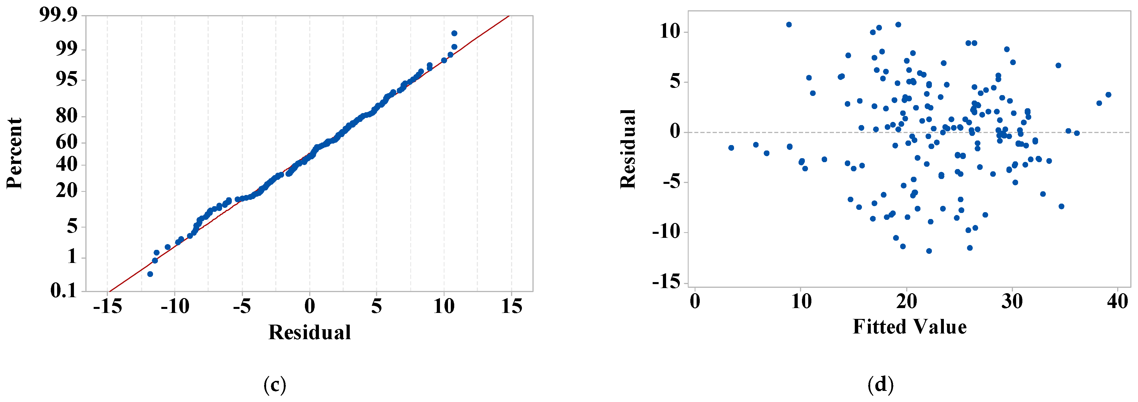
2.3. Modeling and Dataset Preparation

Existing predictive equations for the mechanical properties of GPC are often derived from individual experimental datasets or limited data pooled from select studies. However, the variability in material sources, curing conditions, and testing protocols across studies restricts the broader applicability of these models. To ensure reliability, such equations must be rigorously validated against large datasets. This underscores the necessity for systematic, large-scale data analysis and the development of globally representative models to accurately characterize GPC’s mechanical behavior.

For this study, a thorough search was conducted to assemble a large dataset encompassing. $f_c^{\prime }$, $f_{st}$, $f_r$, $E$, and σ-ε relationship. The predictive models were developed based on a dataset comprising 726 mix designs sourced from published literature, with the range of the mechanical properties given in

Table 3. Descriptive statistics and outliers, Grubbs’ test of the collected datasets.

Item	Mean	Standard Deviation	Minimum	Maximum	Grubbs’ Test	p
$f_{st}$	3.59	1.10	0.94 MPa	5.92 MPa	2.40	1.000
$f_r$	4.49	1.33	0.62 MPa	7.39 MPa	2.92	0.688
$E$	24.07	8.73	1.87 GPa	47.51 GPa	2.68	1.000
$f_c^{\prime }$	44.26	17.43	13.5 MPa	87.4 MPa	2.47	1.000
Peak ε	0.00252	0.00045	0.00163	0.00363	2.5	0.948
Ultimate ε	0.00602	0.00364	0.00230	0.01658	2.89	0.053

. Only articles published in peer-reviewed journals indexed in Scopus and Web of Science (WoS) were considered. These indexing services serve as a proxy for academic credibility and editorial standards. The primary focus of this study was on pure normal weight FA-based GPC. Therefore, only studies utilizing FA (Both Class F and Class C fly ash) as the sole solid precursor were included. Studies employing blended precursor systems (e.g., FA combined with GGBFS, metakaolin, etc.) or additives (e.g., silica fume, nano silica, etc.) were excluded. Geopolymers primarily activated by combinations of sodium silicate and sodium hydroxide were considered. Only mixes cured under ambient or thermal conditions (≤80 °C) were considered. These constraints define the applicability limits of the proposed models. This methodology ensures the suitability of the compiled dataset for a reliable statistical analysis and model development.

The dataset included 184 datapoints (from 22 references [16,18,19,20,23,24,26,37,38,39,40,41,42,43,44,45,46,47,48,49,50,51,52,53,54]) for $f_{st}$, 216 datapoints (from 20 references [16,24,25,26,38,39,40,41,42,43,44,46,47,48,49,50,52,53,55,56,57]) for $f_r$, 233 datapoints (from 23 references [19,20,24,25,26,38,39,40,43,44,45,48,49,50,51,53,54,55,56,58,59,60]) for $E$, and 93 datapoints (from 9 references [16,54,61,62,63,64,65,66,67]) for σ-ε relationship. Table 3 provides the descriptive statistics of the collected datasets. An outlier Grubbs’ test was conducted over each item, and the results revealed that no outliers are present in any dataset at the 0.05 level of significance.

Many proposed models are often based on limited sample sizes and overlook the influence of specimen geometry (size and shape) on strength measurements. To enable accurate comparisons, conversion factors must be applied to standardize results across varying specimen dimensions. However, such adjustments are rarely implemented in existing studies. Due to the absence of research quantifying geometry effects on GPC strength, conversion factors derived for OPC concrete, as summarized in

Table 4. Factors of conversion to a standard 15 × 30 cm cylindrical specimen [68,69].

Strength Grade (MPa)	Shape and Size of Specimen
	Cylinder 10 × 20 cm	Cube 10 cm	Cube 15 cm
$f_{st}$	0.901	0.825	0.915
G20–40 $f_c^{\prime }$	0.971	0.762	0.800
$\mathrm{G}50f_c^{\prime }$	0.971	0.790	0.830
$\mathrm{G}60f_c^{\prime }$	0.971	0.819	0.860
$\mathrm{G}70f_c^{\prime }$	0.971	0.833	0.875
$\mathrm{G}80f_c^{\prime }$	0.971	0.848	0.890

, were adopted. These factors are multiplied by the measured $f_{st}$ or $f_c^{\prime }$ to normalize results to equivalent 150 × 300 mm cylindrical specimens, as stipulated in standards [68,69].

3. Results and Discussion

Geopolymer binders have shown an increasing potential for use as cement replacement materials in the concrete industry. These binders can produce concrete with a wide range of physical and mechanical properties. In order to prepare GPC with the desired properties, the Si/Al, M/Si (M denotes any alkali cations), and water/binder ratios need to be controlled. Hence, it is required to carefully characterize the alkali activator and the source material to determine these ratios. The models presented in this section are designed primarily for performance estimation within the range of input variables used in the training dataset. Extrapolation beyond the tested parameter ranges, particularly in terms of binder type, activator concentration, and curing conditions, may result in reduced prediction accuracy.

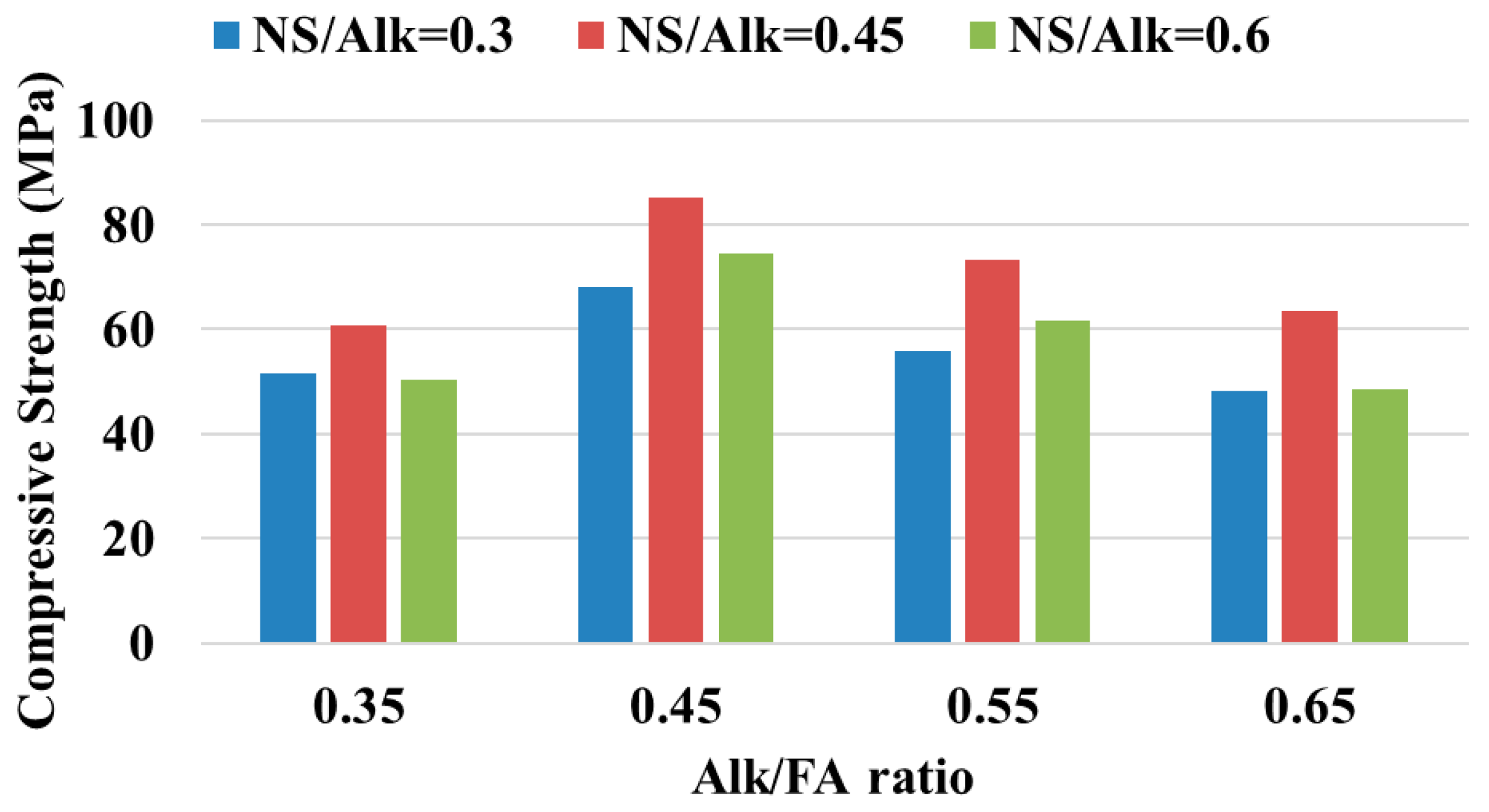
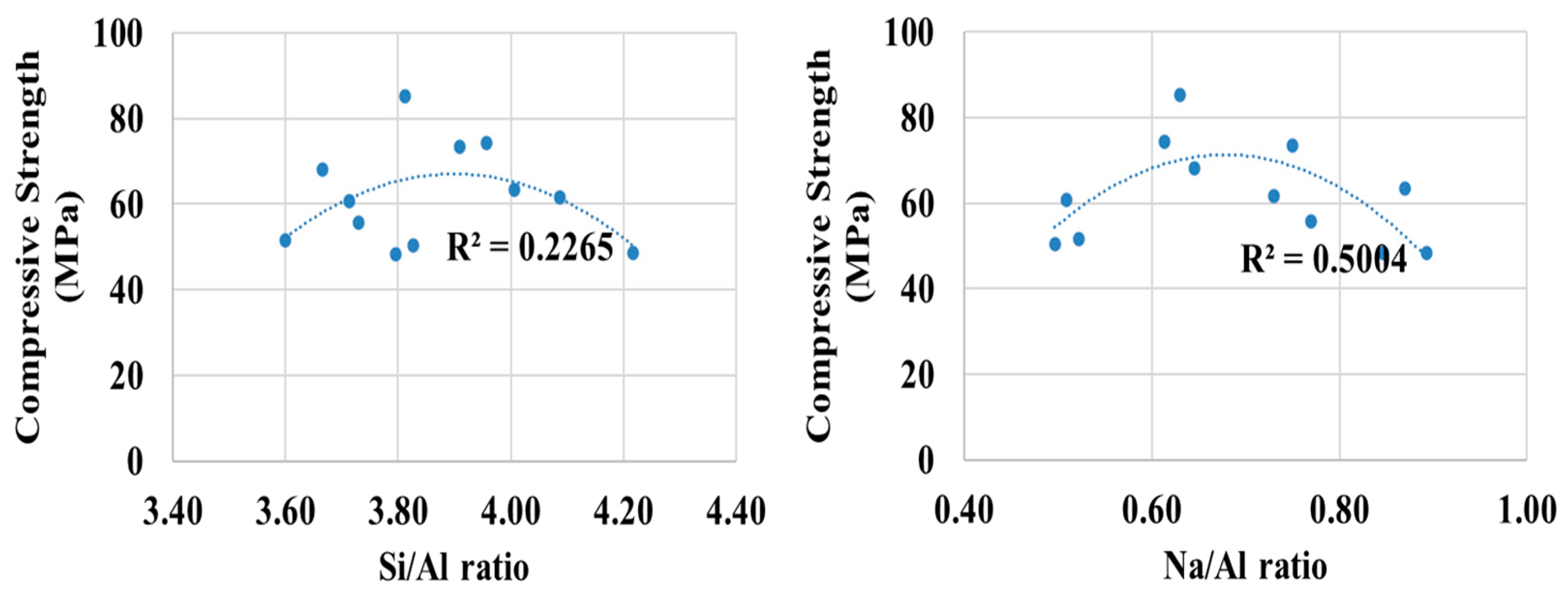
3.1. Compressive Strength

Figure 1 shows the effect of Ns/Alk and Alk/FA ratios on $f_c^{\prime }$ of GPC. The figure shows a decreasing trend in strength with the Alk/FA ratio increasing. This is true except for Alk/FA = 0.35, which could be attributed to poor workability. This was noticed especially for the mixture with NS/Alk = 0.6, where higher viscosity was brought by the more NS introduced to the mixture. This was noted during the casting process and after testing, where large, entrapped air bubbles were found within the specimens. Moreover, low Alk/FA ratios have reduced strength due to unreacted fly ash and poor gel connectivity, while high Alk/FA ratios result in strength drops due to capillary pores as water evaporates, shrinkage cracks, and diluted Si/Al monomers forming a less dense gel [33,35].

The figure also shows that increasing the amounts of dissolved silicate in the activation solution has increased geopolymer strength; however, an optimum value is noticed at NS/Alk = 0.45 for all Alk/Fa ratios. Many researchers have investigated the effect of the NH/NS ratio on geopolymer concrete strength [70,71]. Increasing the NS content increases the silicate concentration while reducing the overall sodium ion contribution. This is because NS contains approximately 28.99% silicate and 14.31% sodium, compared to 17.53% sodium by weight in NH. Consequently, higher compressive strength can be achieved by promoting the formation of stronger Si–O–Si bonds during geopolymerization. However, the excess content of silicate will increase the precipitation rate of the aluminosilicate gel at early ages, which will hinder the polycondensation process and produce a feeble structure; hence, lower strength will be achieved [72]. On the other hand, increasing the soluble silicate content is known to reduce the extent of source material reactions due to the higher solution viscosity and drop in the solution alkalinity. Therefore, higher amounts of unreacted particles will remain as deficient places in the geopolymer structure [73,74]. Moreover, the higher ratios of NS/Alk will reduce the amount of Na ions. Such ions play critical roles in dissolving aluminosilicate precursors and balancing charges in the aluminosilicate framework.

Figure 2 shows the relationship between $f_c^{\prime }$ and the parameters investigated in terms of Si/Al and Na/Al ratios. The figure shows that the Si/Al ratio is a critical parameter in GPC, balancing cross-linking and bond strength. An optimal ratio ensures a well-polymerized, dense microstructure, maximizing $f_c^{\prime }$. Deviations from this ratio compromise structural integrity through inadequate networking or unreacted material, underscoring the need for precise mix design [35,75]. On the other hand, the Na/Al ratio governs aluminosilicate dissolution efficiency and charge balance in the geopolymer network. Balanced Na/Al ensures strong, dense N-A-S-H gel formation, maximizing $f_c^{\prime }$. Extreme ratios degrade performance through unreacted material, efflorescence, or unstable gels [76,77]. An observable trend was noted between the Si/Al molar ratio and compressive strength, with peak values generally occurring in the range of 3.8 to 4.0. However, due to the low coefficient of determination ($R^2$= 0.23), this should be interpreted as a preliminary trend rather than a definitive optimum. A second-order polynomial fit was applied to highlight potential non-linear behavior. The figure also shows that Na/Al provided a stronger relationship ($R^2$= 0.5) with peak values generally occurring in the range of 0.6 and 0.75.

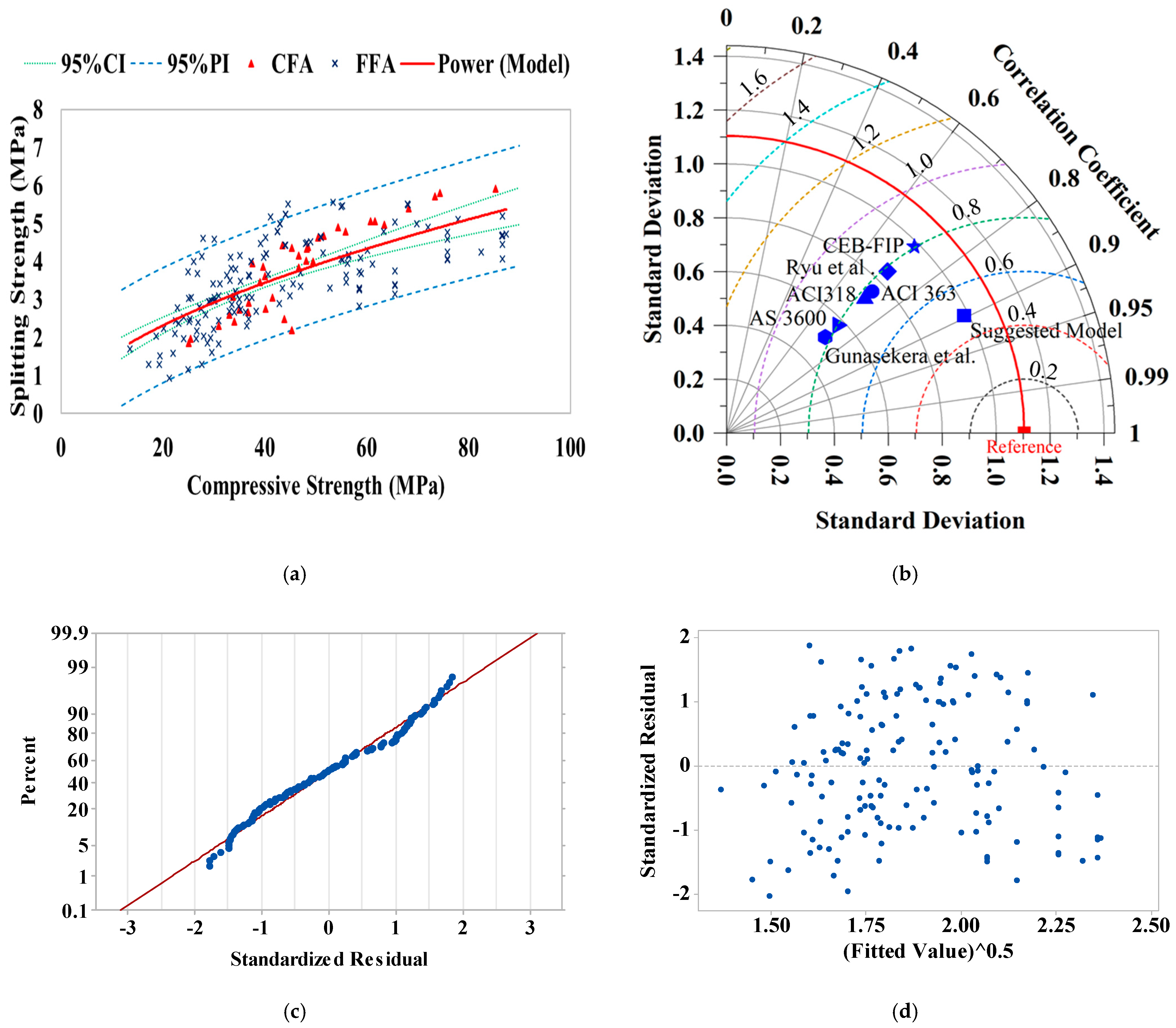
3.2. Splitting Tensile Strength

Several models have been proposed to determine the relationship between $f_{st}$ and $f_c^{\prime }$ of GPC. Most of these models are similar in form to the currently available OPC concrete models in which $f_{st}$ is related to $f_c^{\prime }$ by the power formula given by $f_{st}=m{f_c^{\prime }}^n$ where (m) and (n) are the relationship coefficients obtained by regression analysis of experimental results.

Table 5. Values of regression constants of $f_{st}$ models for GPC and OPC concrete.

Reference	m	n	Reference	m	n
CEB-FIP [78] (OPC)	0.30	0.67	ACI 363 [79] (OPC)	0.59	0.50
AS 3600 [80] (OPC)	0.4	0.5	ACI318 [15] (OPC)	0.56	0.50
Ryu et al. [23] (GPC)	0.17	0.75	Gunasekera et al. [38] (GPC)	0.45	0.50
Luan et al. [37] (GPC)	0.203	0.722	Lee et al. [81] (GPC)	0.47	0.52
Dissanayake [82] (GPC)	0.27	0.67	Jindal et al. [83] (GPC)	0.426	0.519
Albitar et al. [16] (GPC)	0.6	0.5	Thomas et al. [22] (GPC)	0.40	0.778

shows the values of m and n as adopted by some design standards for OPC concrete and suggested by some researchers for FA-based GPC. As given by Table 5, these factors varied between ${\displaystyle \frac{1}{5}}$ to ${\displaystyle \frac{3}{5}}$ and ${\displaystyle \frac{2.5}{5}}$ to ${\displaystyle \frac{4}{5}}$ for (m) and (n) coefficients, respectively.

Figure 3a shows a scatter plot of $f_{st}$ versus $f_c^{\prime }$ for the collected dataset. The $f_c^{\prime }$ ranged between 13.5 MPa and 89.4 MPa with a mean value and a standard deviation of 44.7 MPa and 17.96, respectively. While the $f_{st}$ ranged between 0.94 MPa and 7.43 MPa with a mean value and a standard deviation of 3.66 MPa and 1.21, respectively. The ratio between $f_{st}$ and $f_c^{\prime }$ ranged between 5 and 15%. The regression analysis provided the presence of 6 datapoints classified as outliers; these points were excluded, and a power regression model was determined as given by Equation (1). Figure 3a shows the trend line of the proposed model and its 95% confidence interval (95% CI) and 95% prediction interval (95% PI).

$$f_{st}=0.47{f_c^{\prime }}^{0.57}$$

(1)

Using this model, the values of $R^2$, $R^2$(adj), and $R^2$(pred) were 62.18%, 61.93%, and 61.14%, respectively. The small difference (<0.2%) between predicted and adjusted $R^2$ indicates an adequate signal and design space navigation capability. Also, a large F-value of 254.62 and <0.000 p-value indicates the significance of the proposed model. Figure 3c,d shows that the residuals by using the suggested model were nearly following a normal distribution, and the predictions provided a constant range of residuals across the plot, respectively indicating the goodness of fitting. It is important to recognize that these models predict only the average strength. Given the inherent variability in concrete strength, the 95% prediction interval (particularly its lower bound) is critical for structural design. This interval indicates a 95% probability that the actual strength lies within the specified range. The lower limit (characteristic strength) represents a value with a 95% confidence level that the true strength exceeds, serving as a safety threshold. While the $R^2$ value may appear low, statistical significance is maintained (p-value < 0.0001), and such $R^2$ value is considered large enough for the 184-data-point dataset [84]. Figure 3a demonstrates that almost 100% of the results fall within the prediction interval. For design purposes, the lower prediction limit is recommended to account for safety margins, as it approximates 70% of the mean strength. This aligns with practices for OPC concrete, where standards such as CEB-FIP similarly define the tensile strength lower limit as 70% of the mean [78], suggesting comparable variability between FA-based GPC and OPC concrete. It is worth noting that the effect of FA type, Class C CFA or Class F (FFA), is not critical on $f_{st}$–$f_c^{\prime }$ relationship as can be seen from Figure 3a. The observed similarity in regression equations suggests that FA type has little influence on the $f_{st}$–$f_c^{\prime }$ relationship. Consequently, the data can be simplified using a single power Equation (1).

Figure 3b presents a Taylor diagram comparing the performance of several predictive models, including those suggested by current OPC concrete standards and various literature models detailed in Table 5, against a reference dataset. In this diagram, the “Reference” point (the red square) represents the observed data, against which all models are evaluated. The plot clearly demonstrates that the suggested model (blue square) exhibited superior performance compared to the other evaluated models. It was positioned notably closer to the “Reference” point, indicating a higher degree of agreement with the observed data. Specifically, the suggested model yielded the lowest root mean square deviation (RMSD), visually falling within the 0.4–0.6 RMSD contour from the reference. This is a significant improvement when compared to other models, which generally show RMSD values ranging from approximately 0.6 to 0.8. Furthermore, the suggested model achieved the highest correlation coefficient of approximately 0.9, in contrast to the other models, whose correlation coefficients typically range from 0.65 to 0.75. This indicates the superior goodness-of-fit and predictive capability of the suggested model when compared to existing approaches.

The $f_{st}$ of the tested GPC specimens ranged between 4.6 and 6.5 MPa. Similar to $f_c^{\prime }$, the average $f_{st}$ of concrete is largely determined by its mixing proportions. Figure 4 shows that $f_{st}$ increased as $f_c^{\prime }$ increased; however, the rate of increase showed a decreasing trend (the rate of increase slowed down at $f_c^{\prime }$ values). The ratio of the main $f_{st}$/$f_c^{\prime }$ in this experiment was between 7% and 10%. Generally, the figure shows that the $f_{st}$ of GPC in this study was higher than predicted by the ACI [15,79] and CEB-FIP [78] model codes for both normal and high-strength OPC concrete. This can be attributed to the enhanced interfacial transition zone (ITZ) between the geopolymer binder and aggregates, as documented in multiple studies. Notably, Lee et al. [81] observed that geopolymers formulated with elevated hydroxide concentrations and silicate-rich activators exhibited stronger ITZ bonding, primarily due to reduced porosity in the geopolymer matrix [17,18]. Additionally, in systems containing calcium-rich compounds, the calcium silicate hydrate (C-S-H) phases form within voids of the aluminosilicate network, leading to a denser, lower-porosity matrix that enhances mechanical strength [19,20]. The figure also shows that while the proposed model underestimates the experimental values, it provides a closer approximation than can be determined from the standard equations.

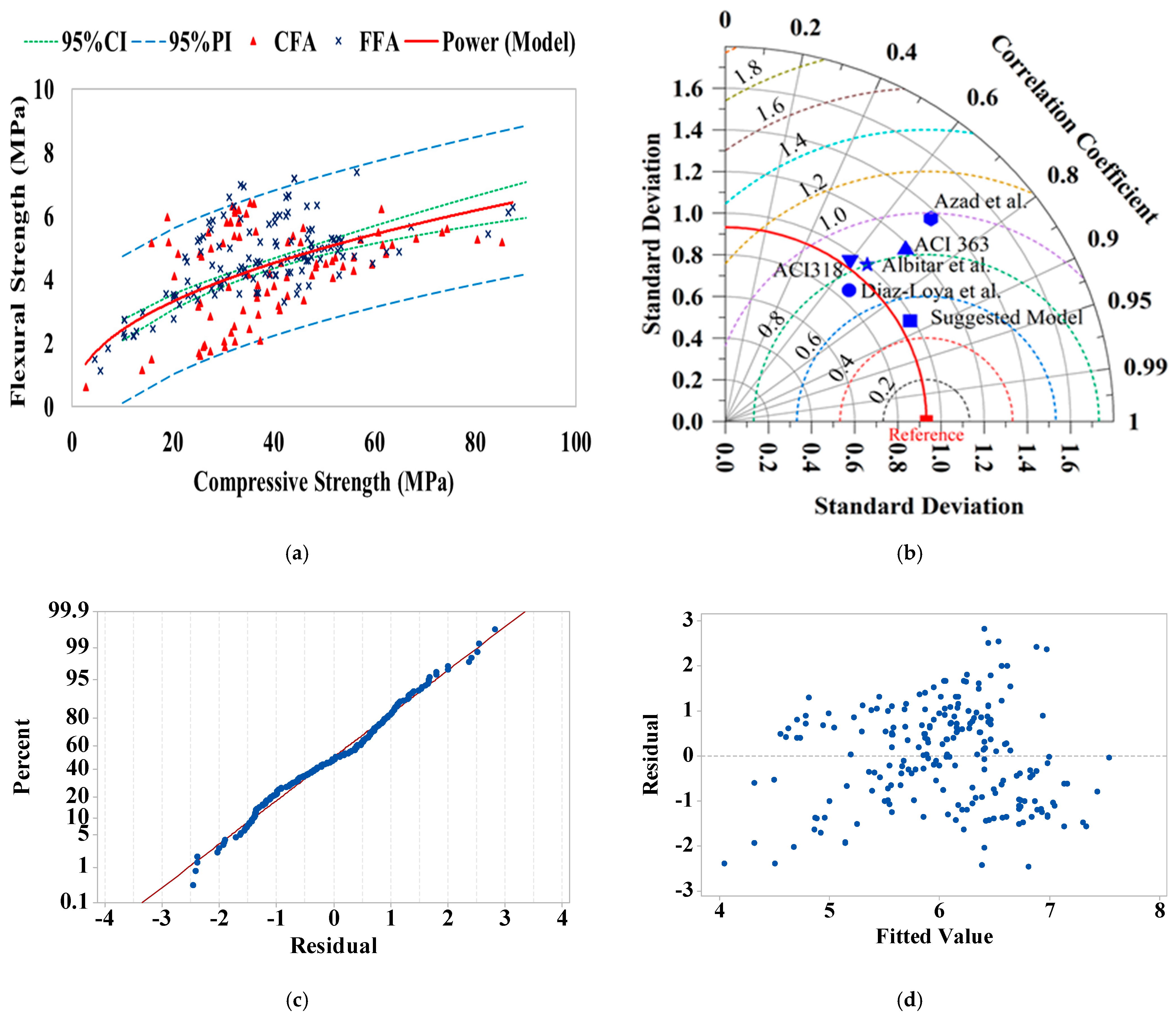
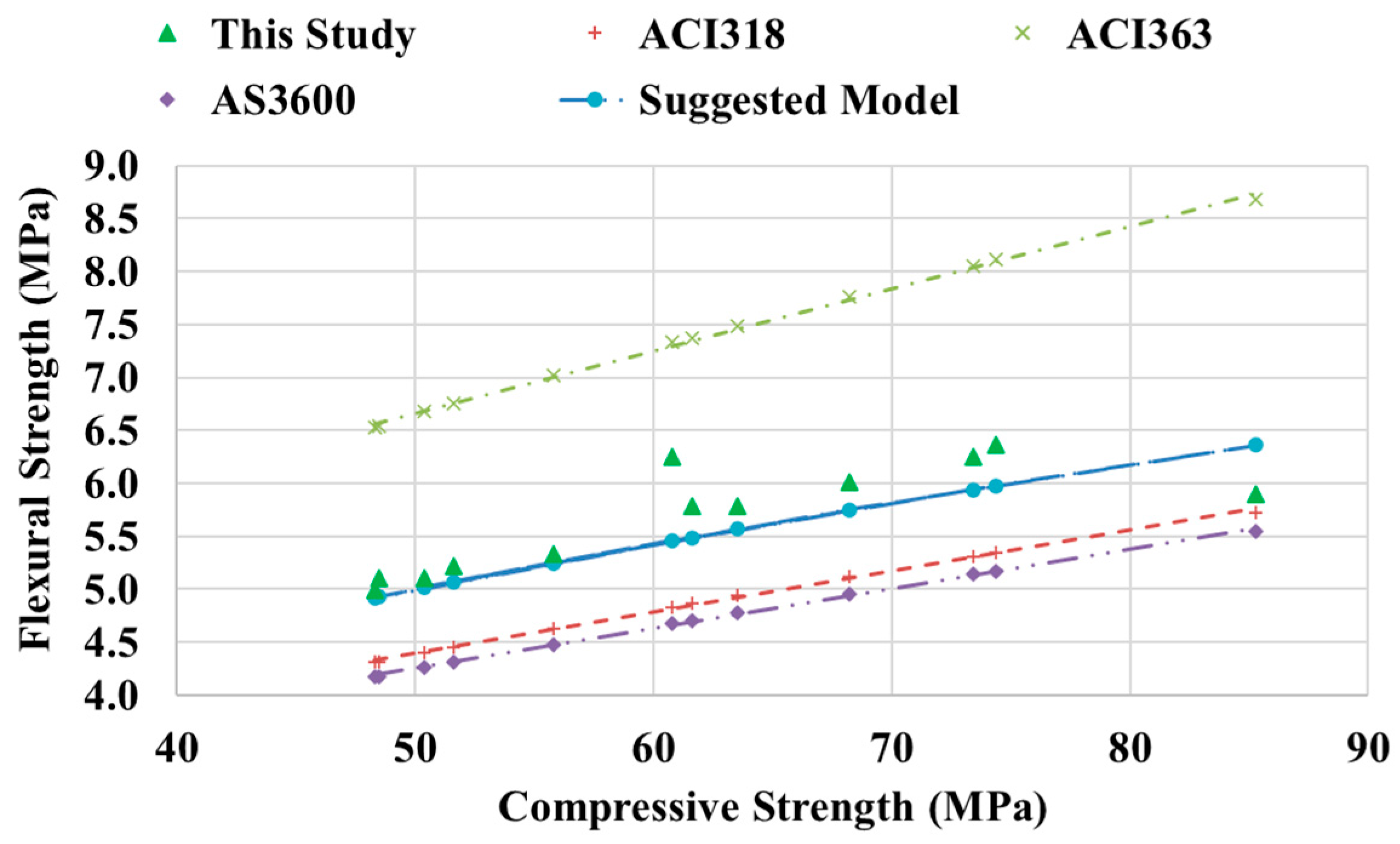
3.3. Flexural Strength

Several models have been proposed to determine the relationship between $f_r$ and $f_c^{\prime }$ of GPC. Most of these models are similar in form to the currently available OPC concrete power.

Table 6. Values of regression constants of $f_r$ models for GPC and OPC concrete.

Reference	m	n	Reference	m	n
ACI 363 [79] (OPC)	0.94	0.5	AS 3600 [80] (OPC)	0.6	0.5
ACI318 [15] (OPC)	0.62	0.5	Gunasekera et al. [38] (GPC)	0.7	0.5
Albitar et al. [16] (GPC)	0.75	0.5	Azad et al. [63] (GPC)	0.293	0.765
Diaz-Loya et al. [24] (GPC)	0.69	0.5	Islam R. et al. [48] (GPC)	0.64	0.5
Gomaa E. et al. [52] (GPC)	0.65	0.5	Nath P. et al. [56] (GPC)	0.93	0.5

shows the values of regression coefficients for the power model as suggested by the design standards (for OPC concrete) and literature.

Figure 5a shows a scatter plot of $f_r$ versus $f_c^{\prime }$ for the collected dataset. The $f_c^{\prime }$ ranged between 2 MPa and 88 MPa with a mean value and a standard deviation of 38.17 MPa and 15.18, respectively. While the $f_{st}$ ranged between 0.62 MPa and 7.39 MPa with a mean value and a standard deviation of 4.92 MPa and 1.33, respectively. The ratio between $f_r$ and $f_c^{\prime }$ ranged between 5 and 33%. The regression analysis of the collected dataset provided the presence of 5 readings classified as outliers; these points were excluded, and a power regression model Equation (2) was determined.

$$f_r=0.86{f_c^{\prime }}^{0.45}$$

(2)

Using this model, the values of $R^2$, $R^2$(adj), and $R^2$(pred) were 67.47%, 67.13%, and 65.90%, respectively. The $R^2$ value is large enough since regression was conducted on a large dataset, including more than 200 data points. In addition, the statistical significance of the model is maintained where its p-value is less than 0.0001. The small difference (<0.2%) between predicted and adjusted $R^2$ indicates an adequate signal and design space navigation capability. Also, a large F-value of 85.16 and <0.000 p-value indicates the significance of the proposed model. Figure 3c,d shows that the residuals were nearly following a normal distribution, and the predictions provided a constant range of residuals across the plot, respectively indicating the goodness of fitting. Figure 5a shows that most of the readings were located within the model’s 95% prediction intervals, indicating that the model provides reliable predictions, as it accurately reflects the variability of the data. The Taylor diagram depicted in Figure 5b indicates the superior goodness-of-fit and predictive capability of the suggested model when compared to existing approaches. The suggested model provided the lowest RMSD of about 0.45 and the highest correlation coefficient of approximately 0.88. The plot clearly demonstrates that the suggested model (blue square) exhibits superior performance compared to the other evaluated models, as given by Table 6.

The $f_r$ follows the general trend of $f_{st}$ and affected by the same variables affecting the $f_c^{\prime }$, where the GPC flexural strength increased as the $f_c^{\prime }$ increased. The $f_r$ of GPC is generally higher than for OPC concrete. This can be seen from Figure 5a, whereas the ACI 318 model is close to the lower bound of the suggested model. The same note is applied to the AS3600 model. On the other hand, the ACI363 model for high-strength concrete tends to overestimate the $f_r$. This trend is also clear based on the results of the tested specimens in this study, as depicted in Figure 6. The $R^2$ values for all these standard models were less than 30%. Similar to $f_{st}$–$f_c^{\prime }$ relationship, FA type is not critical on $f_r$–$f_c^{\prime }$ relationship, and this relationship can be simplified using a single power Equation (2). Good predictions can be obtained using Equation (2), as depicted in Figure 6. This equation tends to give acceptable predictions with some safety margins.

3.4. Modulus of Elasticity

As for the OPC concrete, the modulus of elasticity of GPC is dependent on its constituent proportions, aggregate properties, and curing conditions, and is directly proportional to its $f_c^{\prime }$. Several models have been proposed to determine the relation between $E$ and $f_c^{\prime }$ of GPC as shown in

Table 7. Models for estimation of the elasticity modulus in MPa.

Reference	Model
CEB-FIP [78] (OPC)	$E=21500{\alpha }_E\sqrt[3]{{\displaystyle \frac{f_c^{\prime }}{10}}}$ $\mathrm{where}{\alpha }_E$ is a factor ranging from 0.7 to 1.2 to consider the effect of aggregate type
ACI318 [15] (OPC)	$0.043{\rho }_c^{1.5}\sqrt{f_c^{\prime }}$ $\mathrm{where}{\rho }_c$ $\mathrm{is}\mathrm{the}\mathrm{density}({\displaystyle \frac{\mathrm{k}\mathrm{g}}{{\mathrm{m}}^3}}$)
ACI 363 [79] (OPC)	$3320\sqrt{f_c^{\prime }}+6900$
AS 3600 [80] (OPC)	$E=\left\{\begin{array}{cc}\hfill 0.043{\rho }_c^{1.5}\sqrt{f_c^{\prime }},& f_c^{\prime }\le 40\hfill \\ \hfill {\rho }_c^{1.5}(0.024\sqrt{f_c^{\prime }}+0.12),& f_c^{\prime }>40\hfill \end{array}\right.$
Gunasekera et al. [38] (GPC)	$0.024{\rho }_c^{1.5}\sqrt{f_c^{\prime }}$
Diaz-Loya et al. [24] (GPC)	$580\sqrt{f_c^{\prime }}$
Nath and Sarker [56] (GPC)	$3510\sqrt{f_c^{\prime }}$
Lee and Lee (GPC) [85]	$5300\sqrt{f_c^{\prime }}$
Hassan and Shariq [44] (GPC)	$4100\sqrt{f_c^{\prime }}$

. Most of these models were proposed based on limited experimental work. On the other hand, the available design equations for OPC tend to overestimate the modulus of elasticity of GPC, and hence, these equations shall be modified.

The correlation between static elastic modulus and compressive strength is represented by a regression model shown in Figure 7. Figure 7a shows that the use of the current available design models of ACI 318 code [86], ACI 363 [79], and AS 3600 [80] will generally overestimate the modulus of elasticity of GPC. However, in the case of CFA-based GPC, these design models may provide good predictions with $R^2$ value around 50%. The regression analysis of the dataset shown in Figure 7a returned the following general model for both CFA and FFA-based GPC.

$$E={{1.17f}_c^{\prime }}^{0.81}$$

(3)

Using this model, the values of $R^2$, $R^2$(adj), and $R^2$(pred) were 66.11%, 65.95%, and 65.32%, respectively. Regression on a large dataset (over 200 points) yielded a statistically significant model (p < 0.0001, large F-value > 300) with minimal difference between predicted and adjusted R-squared (<0.2%), indicating good signal and model significance. Figure 7 shows the residual analysis (normal distribution, constant range) and most data points within 95% prediction intervals, confirming the model’s goodness of fit and reliable predictions. Moreover, with the lowest RMSD of about 0.41 and the highest correlation coefficient of approximately 0.87, the Taylor diagram depicted in Figure 7b indicates the goodness-of-fit and predictive capability of the suggested model when compared to existing approaches.

Since CFA and FFA-based GPC provided different trends, the following models can be proposed to predict the elasticity modulus of GPC. By applying Equation (4) to the same dataset (including 55 and 178 datapoints on CFA and FFA, respectively), the $R^2$ values will be 66.66% and 70.71% for CFA and FFA-based GPD, respectively. The application of these models can provide better predictions.

$$E=\left\{\begin{array}{ll}{{1.52f}_c^{\prime }}^{0.78},& CFA-basedGPC\\ {{1.09f}_c^{\prime }}^{0.81},& FFA-basedGPC\end{array}\right.$$

(4)

Diaz-Loya et al. [24] have suggested that any proposed model for the estimation of the modulus of elasticity of GPC shall include a term for density ($\mathsf{\rho }$) and $f_c^{\prime }$ interaction to reduce the variability in the predicted values. Given that the GPC samples exhibited a wide range of density values, another regression model was derived using both $\mathsf{\rho }$ (${\mathrm{k}\mathrm{g}/\mathrm{m}}^3$) and $f_c^{\prime }$ (MPa) as independent variables. The regression analysis was conducted on only 92 datapoints with known density. The model is given by a second-order polynomial function Equation (5), and it provided $R^2$, $R^2$(adj), and $R^2$(pred) values of 84.17%, 83.24, and 82.30%, respectively. The remaining performance indicators showed satisfactory goodness of fit and design space navigation. This suggests that the incorporation of density into the prediction model aids in capturing the variability observed in the elastic modulus of FA-based GPC, as can be seen from Figure 8.

$$E\left(GPA\right)=1607.67-1.51\mathsf{\rho }-25.97f_c^{\prime }+0.024\mathsf{\rho }{f}_c^{\prime }+0.00036{\rho }^2-5.63\times {10}^{-6}{f}_c^{\prime }{\mathsf{\rho }}^2$$

(5)

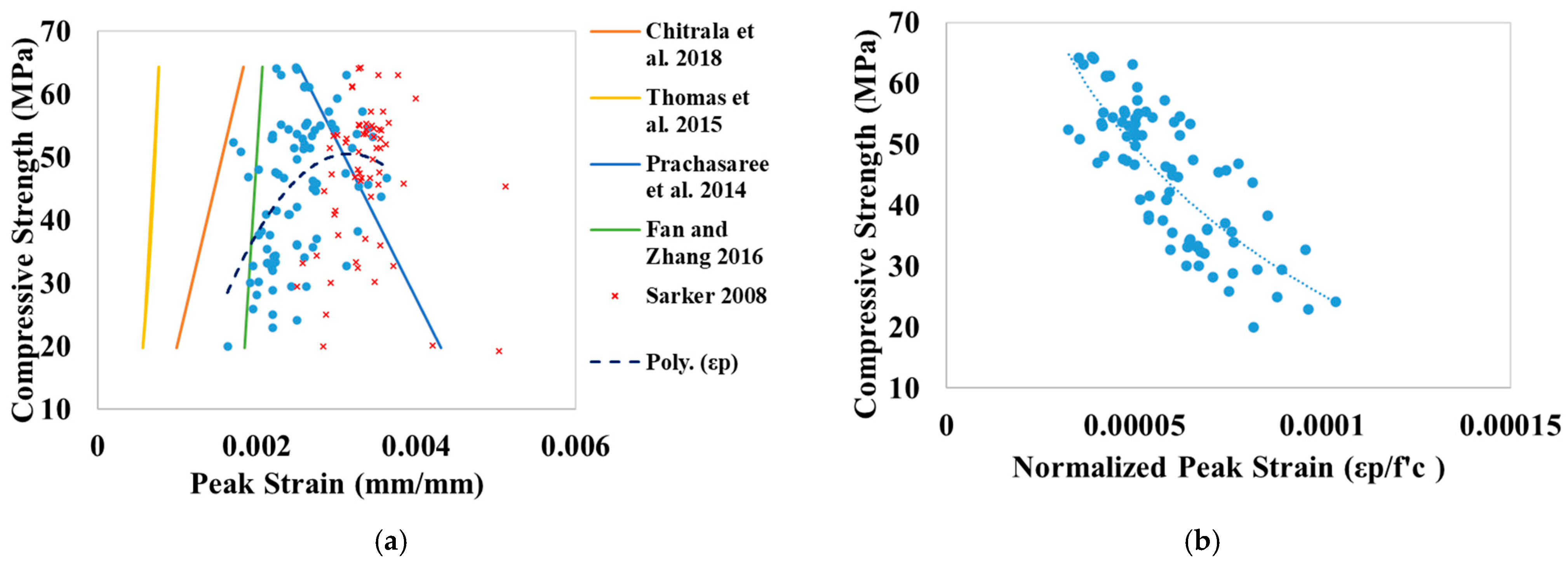
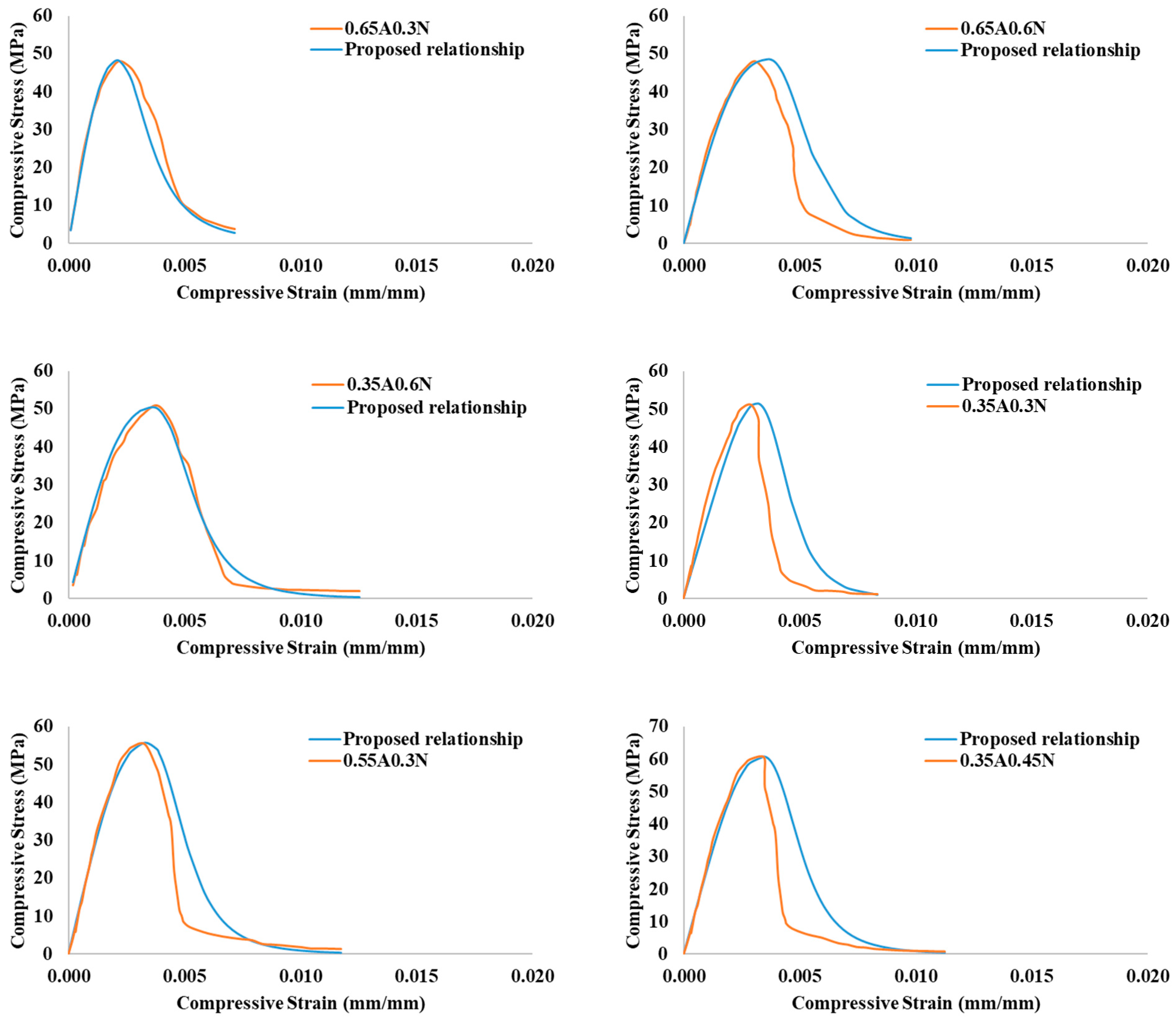
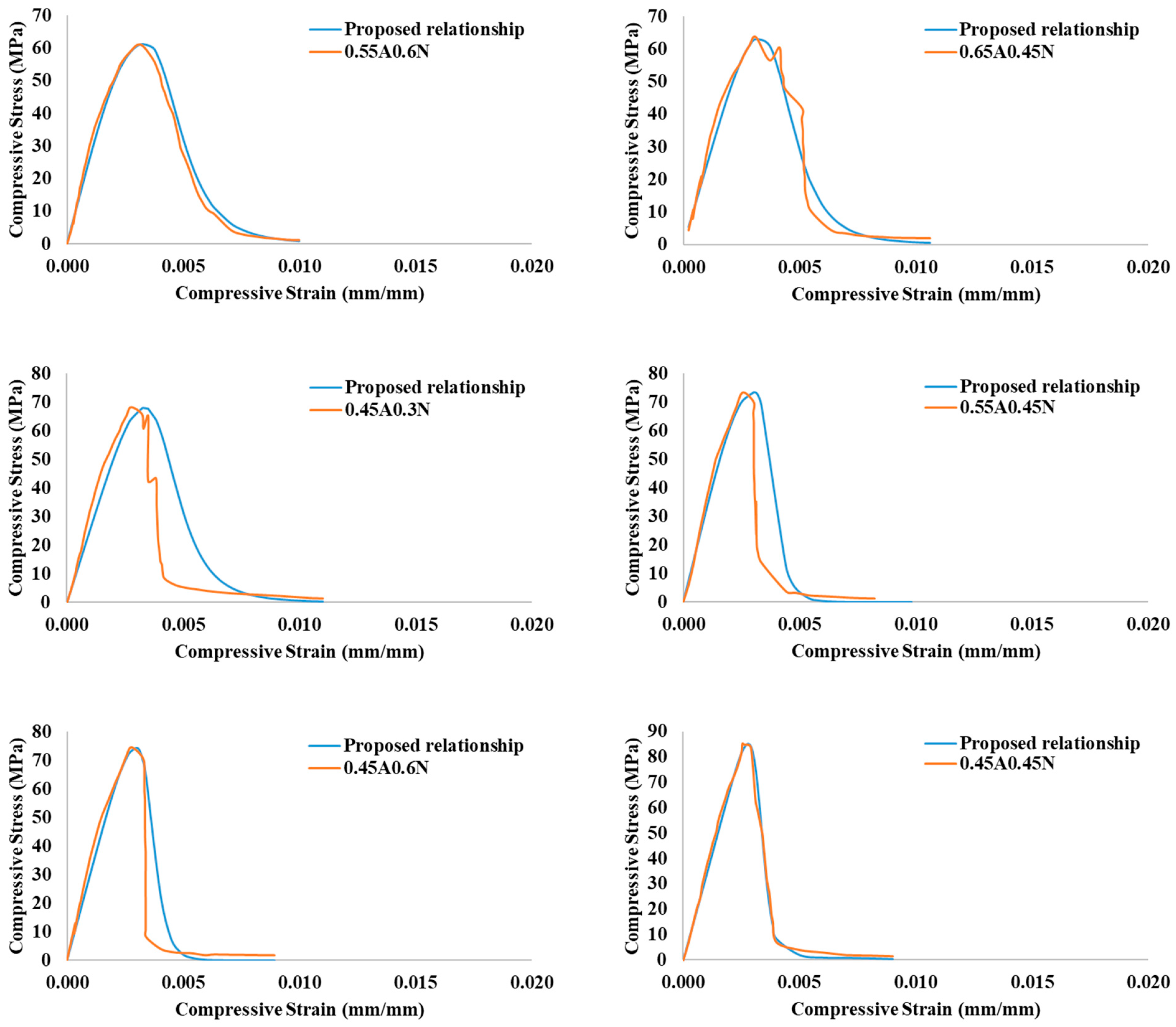
3.5. Stress–Strain Relationship

The determination of the ascending (pre-peak) and descending (post-peak) portions of the stress–strain relationship ($\sigma -\epsilon$) requires the knowledge of some essential parameters, including elasticity modulus, linearity index of the pre-peak portion of $\sigma -\epsilon$, peak strain (${\epsilon }_p$), and ultimate strain (${\epsilon }_u$) should be first estimated. A better representative model of the elasticity modulus was determined in the previous section. However, it is still required to find a proper model for the peak strain (${\epsilon }_p$) of GPC. This property is of paramount importance in determining a representative $\sigma -\epsilon$ of GPC.

The linearity index of the ascending portion of $\sigma -\epsilon$ can be estimated as the ratio between the initial tangent modulus of elasticity and the secant modulus measured at the peak stress. This ratio is usually around 2 for OPC concrete of normal strength and close to 1 for high-strength concrete [61]. In the case of FA-GPC, considering the dataset collected from the literature and the results obtained in this study (a total of 97 datapoints), the linearity index ranged from 0.89 to 1.81 with an average of 1.29. The lower index value for FA-GPC indicates a more linear elastic behavior up to the peak stresses. The higher the value above 1, the more pronounced the non-linearity and stiffness reduction before reaching peak stress. The linearity index is found to be proportional to $f_c^{\prime }$ and its value approach to unity as $f_c^{\prime }$ increases.

Several models were suggested to determine ${\epsilon }_p$ of GPC as given in

Table 8. Experimental models for estimation of peak and ultimate strain of GPC.

References	Peak Strain Models	Ultimate Strain Models
Chitrala et al. [87]	${\epsilon }_p=\left(18.97f_c^{\prime }+623.60\right)\times {10}^{-6}$	${\epsilon }_u=(2.8-0.05\ln f_c^{\prime }){\epsilon }_p$
Sarker [88]	${\epsilon }_p={\displaystyle \frac{f_c^{\prime }}{E}}+{\displaystyle \frac{0.8{+f}_c^{\prime }/12}{(0.8{+f}_c^{\prime }/12)-1}}$	Not applicable
Thomas et al. [22]	${\epsilon }_p=2.7\times {10}^{-4}{f_c^{\prime }}^{0.25}$	Not applicable
Prachasaree et al. [67]	${\epsilon }_p=0.0051-4\times {10}^{-5}{f}_c^{\prime }$	Not applicable
Fan and Zhang [89]	${\epsilon }_p=0.002+0.5\left(f_c^{\prime }-50\right)\times {10}^{-5}$	${\epsilon }_u=0.0033+0.5\left(f_c^{\prime }-50\right)\times {10}^{-5}$

. The ${\epsilon }_p$ predictions using these models over the collected dataset provided a low correlation of these models as shown in Figure 9a. Using regression analysis, a second-order polynomial model is the best fit for the collected dataset. However, this model will also provide a low determination coefficient of only $R^2$= 18.89%. Hence, another regression model, Equation (6), was proposed using normalized peak strain (${\epsilon }_p/f_c^{\prime }$) and compressive strength as shown in Figure 9b. This model provided a good determination coefficient of $R^2$= 62.77% with a mean (tested/predicted) value of 1.19, indicating the goodness of this model with safety of margins.

$${\displaystyle \frac{{\epsilon }_p}{f_c^{\prime }}}=-4\times {10}^{-5}\mathit{ln}{f}_c^{\prime }+0.0002$$

(6)

Few studies were found in the literature regarding the ultimate strain (${\epsilon }_u$) of FA-GPC. Some of the suggested models are given in Table 8. Considering the collected dataset, a low correlation was found between $f_c^{\prime }\mathrm{a}\mathrm{n}\mathrm{d}{\epsilon }_u$, the data points were highly scattered, and any regression analysis was found to provide a low determination coefficient ($R^2$< 10%). The same thing was noted even when normalization was used. Nevertheless, regression analysis was conducted over the data collected from this study. To increase the model goodness, the elasticity modulus was also included in the regression analysis. The analysis yielded Equation (7) with $R^2$= 69.65%.

$${\epsilon }_u={\displaystyle \frac{2.23\times {10}^{-7}{E}^{1.67}\left[3.5-0.05\mathit{ln}\left(f_c^{\prime }\right)\right]}{\left({f_c^{\prime }}^{1.98}\right)}}$$

(7)

The uniaxial compression stress–strain relationships for both ascending and descending portions were suggested using non-linear regression analysis and based on the proposed models for the elasticity modulus and peak and ultimate strains. A full stress–strain diagram can be drawn using Equations (8) and (9). In these equations, ${\sigma }_c$ represents GPC stress (MPa) at any point, $n$ is a parameter of GPC properties used as $n_1$ and $n_2$ to draw the ascending and descending parts of the σ-ε curve, respectively.

$$n=\left\{\begin{array}{cc}\hfill n_1={\left[1-1.15({\displaystyle \frac{\frac{f_c^{\prime }}{0.7{\epsilon }_p}}{E_c}})\right]}^{-0.45}& ,{\epsilon }_c\le {\epsilon }_p\hfill \\ \hfill n_2=n_1+{\displaystyle \frac{15}{\sqrt{11.9-0.008f_c^{\prime }}}}+22.12e^{(-{\displaystyle \frac{800}{f_c^{\prime }}})}& ,{\epsilon }_c>{\epsilon }_p\hfill \end{array}\right.$$

(8)

$${\sigma }_c={\displaystyle \frac{n\left(\frac{{\epsilon }_c}{{\epsilon }_p}\right)}{n-1+{\left(\frac{{\epsilon }_c}{{\epsilon }_p}\right)}^n}}$$

(9)

These equations were used to draw σ-ε curves of the tested specimens, and their results were compared with the experimental measurements as shown in Figure 10. The figures show the goodness of the proposed models. The ascending parts, stress and strain at peaks, and the ultimate strains of all tested specimens were almost identical. However, the descending portion showed small deviations. These deviations were higher in the case of specimens with higher Si/Al ratios. Considering the plots of 0.65A0.3N and 0.65A0.6N, both specimens provided almost similar strength; however, the descending part of the 0.65A0.3N specimens with a Si/Al ratio of 3.79 was steeper than that of the 0.65A0.6N specimens with a Si/Al ratio of 4.21. There was a 36.5% increase in ultimate strain in the case of 0.65A0.3N specimens. Similar notes can be observed between 0.35A0.45N and 0.55A0.6N plots. The ductility of GPC is largely affected by the Si/Al ratio. Fletcher et al. [90] reported that the use of a Si/Al ratio higher than 24 molars resulted in GPC products that failed in a ductile manner by deformation.

In General, as compared to OPC concrete, the deformation of GPC was observed to be larger; for instance, the strain at peak stress ranged from 0.00216 to 0.00379 with a mean value of 0.00296. On the other hand, the ultimate strain ranged between 0.00717 and 0.01255 with a mean value of 0.01002.

Finally, to validate the proposed models, they were used to predict the experimental data provided by Hardjito et al. [62] as shown in Figure 11. The figure shows that the predictions using the suggested models fairly capture both parts of the σ-ε curves. However, the proposed model’s reliability needs further validation through the acquisition of more stress–strain curves for geopolymer concretes utilizing CFA and FFA.

4. Conclusions

Driven by sustainable development goals, GPC offers a promising, concrete solution. This study presents an enhanced data analysis of geopolymer concrete’s mechanical properties, proposing accurate equations based on a large dataset. These equations have direct applications in the design of GPC structural members and in creating a state-of-the-art overview of the material. The following conclusions can be drawn.

• For design purposes, the lower prediction intervals are recommended to account for safety margins, as they approximate 70% of the mean strength.
• The effect of FA type (CFA or FFA) is not critical on the splitting and compressive strengths relationship. Consequently, a single model can be used to express their relationships with good accuracy. The same note was observed in the case of flexural and compressive strength relationships.
• Design codes for OPC concrete, including ACI 318, ACI 363, and CEB-FIP, are shown to generally underestimate the splitting tensile strength when applied to FA-GPC. Notably, the CEB-FIP code’s predictions are the closest to the actual values.
• Design codes for OPC concrete, including ACI 318 and AS3600, are shown to generally underestimate the flexural tensile strength when applied to FA-GPC, while the ACI363 code’s predictions tend to overestimate the actual values.
• Existing design models for the modulus of elasticity of OPC concrete in ACI 318, ACI 363, and AS 3600 codes generally overestimate its value. However, for CFA-based GPC, these models can offer reasonably good predictions. Given the differing trends observed between CFA and FFA-based GPC, different models were proposed. Moreover, including density in such models is found to increase the model’s accuracy.
• FA-GPC provides more linear elastic behavior up to the peak stresses indicated by its lower linearity index value. On the other hand, the deformation of GPC was observed to be larger with a higher strain rate at peak stresses and higher ultimate strain as compared to OPC concrete.
• While environmental impact and economic feasibility are important considerations in the broader evaluation of GPC, the present study is focused specifically on developing and validating predictive models for its mechanical performance. Detailed environmental or cost analysis is, therefore, beyond the current scope, but it is recommended for future investigations to complement the findings presented here.

References

1. Rissman, J.; Bataille, C.; Masanet, E.; Aden, N.; Morrow, W.R.; Zhou, N.; Elliott, N.; Dell, R.; Heeren, N.; Huckestein, B.; et al. Technologies and policies to decarbonize global industry: Review and assessment of mitigation drivers through 2070. Appl. Energy 2020, 266, 114848. [Google Scholar] [CrossRef]
2. The International Energy Agency (IEA). 2025 Statistical Review of World Energy. 2025. Available online: https://www.iea.org/data-and-statistics/charts/global-energy-related-co2-emissions-by-sector (accessed on 22 June 2025).
3. Lee, S. Special Issue: “Recent Developments in Geopolymers and Alkali-Activated Materials”. Materials 2024, 17, 245. [Google Scholar] [CrossRef] [PubMed]
4. Panchami, R.; Deepa Raj, S. Geopolymer Concrete—Advancements, Challenges and Future Prospects. In Technologies for Sustainable Buildings and Infrastructure; Springer: Singapore, 2024; pp. 217–228. [Google Scholar]
5. Alahmari, T.S.; Abdalla, T.A.; Rihan, M.A.M. Review of Recent Developments Regarding the Durability Performance of Eco-Friendly Geopolymer Concrete. Buildings 2023, 13, 3033. [Google Scholar] [CrossRef]
6. AS 3972-2010; General Purpose and Blended Cements. Standards Australia: Sydney, Australia, 2010.
7. EN 206:2013+A2:2021; Concrete—Specification, Performance, Production and Conformity. European Standard: Brussels, Belgium, 2021.
8. ASTM C1897-20; Standard Test Methods for Measuring the Reactivity of Supplementary Cementitious Materials by Isothermal Calorimetry and Bound Water Measurements. ASTM: West Conshohocken, PA, USA, 2020.
9. RILEM TC-283-CAM:2023; Chloride Transport in Alkali-Activated Materials. The International Union of Laboratories and Experts in Construction Materials, Systems and Structures: Champs-sur-Marne, France, 2023.
10. Davidovits, J. State of the Geopolymer R&D. In Proceedings of the Geopolymer Camp 2014, Saint Quentin, France, 7–9 July 2014. [Google Scholar]
11. The World Bank Group. Electricity Production from Coal Sources; International Bank for Reconstruction and Development/The World Bank: Washington, DC, USA, 2024. [Google Scholar]
12. Hamed, Y.R.; Keshta, M.M.; Elshikh, M.M.Y.; Elshami, A.A.; Matthana, M.H.S.; Youssf, O. Performance of Sustainable Geopolymer Concrete Made of Different Alkaline Activators. Infrastructures 2025, 10, 41. [Google Scholar] [CrossRef]
13. Al-Akhras, N.M.; Jamal Shannag, M.; Malkawi, A.B. Evaluation of shear-deficient lightweight RC beams retrofitted with adhesively bonded CFRP sheets. Eur. J. Environ. Civ. Eng. 2016, 20, 899–913. [Google Scholar] [CrossRef]
14. Nuruddin, M.F.; Malkawi, A.B.; Fauzi, A.; Mohammed, B.S.; Almattarneh, H.M. Geopolymer concrete for structural use: Recent findings and limitations. IOP Conf. Ser. Mater. Sci. Eng. 2016, 133, 12021. [Google Scholar] [CrossRef]
15. ACI-318-Committee. Building Code Requirements for Structural Concrete (ACI 318-14) and Commentary; American Concrete Institute: Farmington Hills, MI, USA, 2014. [Google Scholar]
16. Albitar, M.; Visintin, P.; Mohamed Ali, M.S.; Drechsler, M. Assessing behaviour of fresh and hardened geopolymer concrete mixed with class-F fly ash. KSCE J. Civ. Eng. 2014, 19, 1445–1455. [Google Scholar] [CrossRef]
17. Atiş, C.D.; Bilim, C.; Çelik, Ö.; Karahan, O. Influence of activator on the strength and drying shrinkage of alkali-activated slag mortar. Constr. Build. Mater. 2009, 23, 548–555. [Google Scholar] [CrossRef]
18. Sarker, P.K. Bond strength of reinforcing steel embedded in fly ash-based geopolymer concrete. Mater. Struct. 2010, 44, 1021–1030. [Google Scholar] [CrossRef]
19. Hardjito, D.; Rangan, B.V. Development and Properties of Low-Calcium Fly Ash-Based Geopolymer Concrete; Curtin University of Technology: Perth, Australia, 2005; p. 94. [Google Scholar]
20. Topark-Ngarm, P.; Chindaprasirt, P.; Sata, V. Setting Time, Strength, and Bond of High-Calcium Fly Ash Geopolymer Concrete. J. Mater. Civ. Eng. 2015, 27, 4014198. [Google Scholar] [CrossRef]
21. Khalaj, M.-J.; Khoshakhlagh, A.; Bahri, S.; Khoeini, M.; Nazerfakhari, M. Split tensile strength of slag-based geopolymer composites reinforced with steel fibers: Application of Taguchi method in evaluating the effect of production parameters and their optimum condition. Ceram. Int. 2015, 41, 10697–10701. [Google Scholar] [CrossRef]
22. Thomas, R.J.; Peethamparan, S. Alkali-activated concrete: Engineering properties and stress–strain behavior. Constr. Build. Mater. 2015, 93, 49–56. [Google Scholar] [CrossRef]
23. Ryu, G.S.; Lee, Y.B.; Koh, K.T.; Chung, Y.S. The mechanical properties of fly ash-based geopolymer concrete with alkaline activators. Constr. Build. Mater. 2013, 47, 409–418. [Google Scholar] [CrossRef]
24. Diaz-Loya, E.I.; Allouche, E.N.; Vaidya, S. Mechanical properties of fly-ash-based geopolymer concrete. ACI Mater. J. 2011, 108, 300–306. [Google Scholar]
25. Diaz, E.; Allouche, E. Recycling of fly ash into geopolymer concrete: Creation of a database. In Proceedings of the 2010 IEEE Green Technologies Conference, Grapevine, TX, USA, 15–16 April 2010; pp. 1–7. [Google Scholar]
26. Joseph, B.; Mathew, G. Influence of aggregate content on the behavior of fly ash based geopolymer concrete. Sci. Iran. 2012, 19, 1188–1194. [Google Scholar] [CrossRef]
27. Malkawi, A.B. Effect of Aggregate on the Performance of Fly-Ash-Based Geopolymer Concrete. Buildings 2023, 13, 769. [Google Scholar] [CrossRef]
28. Haider, G.M.; Sanjayan, J.G.; Ranjith, P.G. Complete triaxial stress–strain curves for geopolymer. Constr. Build. Mater. 2014, 69, 196–202. [Google Scholar] [CrossRef]
29. Ganesan, N.; Abraham, R.; Deepa Raj, S.; Sasi, D. Stress–strain behaviour of confined Geopolymer concrete. Constr. Build. Mater. 2014, 73, 326–331. [Google Scholar] [CrossRef]
30. Jwaida, Z.; Dulaimi, A.; Mashaan, N.; Othuman Mydin, M.A. Geopolymers: The Green Alternative to Traditional Materials for Engineering Applications. Infrastructures 2023, 8, 98. [Google Scholar] [CrossRef]
31. Khan, Q.S.; Akbar, H.; Qazi, A.U.; Kazmi, S.M.S.; Munir, M.J. Bond Stress Behavior of a Steel Reinforcing Bar Embedded in Geopolymer Concrete Incorporating Natural and Recycled Aggregates. Infrastructures 2024, 9, 93. [Google Scholar] [CrossRef]
32. Sarker, P.K. Analysis of geopolymer concrete columns. Mater. Struct. 2009, 42, 715–724. [Google Scholar] [CrossRef]
33. Nuruddin, M.F.; Malkawi, A.B.; Fauzi, A.; Mohammed, B.S.; Almattarneh, H.M. Evolution of geopolymer binders: A review. IOP Conf. Ser. Mater. Sci. Eng. 2016, 133, 012052. [Google Scholar] [CrossRef]
34. Mahameid, A.; Yasin, A.; Malkawi, A. Prediction of the Compressive and Tensile Strengths of Geopolymer Concrete Using Artificial Neural Networks. Civ. Eng. Archit. 2024, 12, 3193–3206. [Google Scholar] [CrossRef]
35. Winnefeld, F.; Leemann, A.; Lucuk, M.; Svoboda, P.; Neuroth, M. Assessment of phase formation in alkali activated low and high calcium fly ashes in building materials. Constr. Build. Mater. 2010, 24, 1086–1093. [Google Scholar] [CrossRef]
36. Al-Mattarneh, H.; Rawashdeh, A.; Ismail, R.; Matalkah, F.; Alhussien, N.; Malkawi, A. User-Friendly Software System for Geopolymer Concrete Slump and Strength Prediction. In Proceedings of the 2024 IEEE 30th International Conference on Telecommunications (ICT), Amman, Jordan, 24–27 June 2024; pp. 1–7. [Google Scholar]
37. Luan, C.; Wang, Q.; Yang, F.; Zhang, K.; Utashev, N.; Dai, J.; Shi, X. Practical Prediction Models of Tensile Strength and Reinforcement-Concrete Bond Strength of Low-Calcium Fly Ash Geopolymer Concrete. Polymers 2021, 13, 875. [Google Scholar] [CrossRef]
38. Gunasekera, C.; Setunge, S.; Law, D.W. Correlations between Mechanical Properties of Low-Calcium Fly Ash Geopolymer Concretes. J. Mater. Civ. Eng. 2017, 29, 4017111. [Google Scholar] [CrossRef]
39. Olivia, M.; Nikraz, H. Properties of fly ash geopolymer concrete designed by Taguchi method. Mater. Des. 2012, 36, 191–198. [Google Scholar] [CrossRef]
40. Sofi, M.; Van Deventer, J.; Mendis, P.; Lukey, G. Engineering properties of inorganic polymer concretes (IPCs). Cem. Concr. Res. 2007, 37, 251–257. [Google Scholar] [CrossRef]
41. Aliabdo, A.A.; Abd Elmoaty, A.E.M.; Salem, H.A. Effect of cement addition, solution resting time and curing characteristics on fly ash based geopolymer concrete performance. Constr. Build. Mater. 2016, 123, 581–593. [Google Scholar] [CrossRef]
42. Chang, E.H. Shear and bond behaviour of reinforced fly ash-based geopolymer concrete beams. Ph.D. Thesis, Curtin University, Perth, Australia, 2009. [Google Scholar]
43. Nikoloutsopoulos, N.; Sotiropoulou, A.; Kakali, G.; Tsivilis, S. Physical and Mechanical Properties of Fly Ash Based Geopolymer Concrete Compared to Conventional Concrete. Buildings 2021, 11, 178. [Google Scholar] [CrossRef]
44. Hassan, A.; Arif, M.; Shariq, M. Effect of curing condition on the mechanical properties of fly ash-based geopolymer concrete. SN Appl. Sci. 2019, 1, 1694. [Google Scholar] [CrossRef]
45. Shaji, P.; Manoj, A.; Emmanuel, F.; Sreelakshmi, G.; Venu, S.M. Study of Mechanical Properties of Fly Ash Based Geopolymer Concrete. Int. Res. J. Eng. Technol. 2018, 5, 3613–3618. Available online: https://www.irjet.net/archives/V5/i3/IRJET-V5I3847.pdf (accessed on 17 June 2025).
46. Raijiwala, D.B.; Patil, H.S. Geopolymer concrete A green concrete. In Proceedings of the 2010 2nd International Conference on Chemical, Biological and Environmental Engineering, Cairo, Egypt, 2–4 November 2010; pp. 202–206. [Google Scholar]
47. Raijiwala, D.; Patil, H. Geopolymer concrete: A concrete of next decade. J. Eng. Res. Stud. 2011, 2, 19–25. [Google Scholar]
48. Islam, R.; Montes, C.; Allouche, E. Correlation between chemical and phase composition of fly ash and mechanical properties of geopolymer concrete. Int. J. Environ. Eng. Nat. Resour. 2014, 1, 235–239. [Google Scholar]
49. Wardhono, A.; Gunasekara, C.; Law, D.W.; Setunge, S. Comparison of long term performance between alkali activated slag and fly ash geopolymer concretes. Constr. Build. Mater. 2017, 143, 272–279. [Google Scholar] [CrossRef]
50. Gunasekara, M.; Law, D.W.; Setunge, S. The effect of type of fly ash on mechanical properties of geopolymer concrete. In Proceedings of the 27th Biennial National Conference of the Concrete Institute of Australia, Adelaide, Australia, 30 August–2 September 2015; pp. 586–595. [Google Scholar]
51. Pan, Z.; Sanjayan, J.G.; Rangan, B.V. Fracture properties of geopolymer paste and concrete. Mag. Concr. Res. 2011, 63, 763–771. [Google Scholar] [CrossRef]
52. Gomaa, E.; Sargon, S.; Kashosi, C.; Gheni, A.; ElGawady, M.A. Mechanical Properties of High Early Strength Class C Fly Ash-Based Alkali Activated Concrete. Transp. Res. Rec. 2020, 2674, 430–443. [Google Scholar] [CrossRef]
53. Bhikshma, V.; Koti, R.M.; Srinivas, R.T. An experimental investigation on properties of geopolymer concrete (no cement concrete). Asian J. Civ. Eng. 2012, 13, 841–853. [Google Scholar]
54. Nguyen, K.T.; Ahn, N.; Le, T.A.; Lee, K. Theoretical and experimental study on mechanical properties and flexural strength of fly ash-geopolymer concrete. Constr. Build. Mater. 2016, 106, 65–77. [Google Scholar] [CrossRef]
55. Phoo-ngernkham, T.; Phiangphimai, C.; Damrongwiriyanupap, N.; Hanjitsuwan, S.; Thumrongvut, J.; Chindaprasirt, P. A Mix Design Procedure for Alkali-Activated High-Calcium Fly Ash Concrete Cured at Ambient Temperature. Adv. Mater. Sci. Eng. 2018, 2018, 2460403. [Google Scholar] [CrossRef]
56. Nath, P.; Sarker, P.K. Flexural strength and elastic modulus of ambient-cured blended low-calcium fly ash geopolymer concrete. Constr. Build. Mater. 2017, 130, 22–31. [Google Scholar] [CrossRef]
57. Evin; Rachmansyah. The ratio between flexural strength to compressive strength of geopolymer concrete. IOP Conf. Ser. Earth Environ. Sci. 2023, 1195, 012034. [Google Scholar] [CrossRef]
58. Yost, J.R.; Radlińska, A.; Ernst, S.; Salera, M.; Martignetti, N.J. Structural behavior of alkali activated fly ash concrete. Part 2: Structural testing and experimental findings. Mater. Struct. 2013, 46, 449–462. [Google Scholar] [CrossRef]
59. Fernandez-Jimenez, A.M.; Palomo, A.; Lopez-Hombrados, C. Engineering properties of alkali-activated fly ash concrete. ACI Mater. J. 2006, 103, 106–112. [Google Scholar]
60. Hardjito, D.; Sumajouw, D.M.; Wallah, S.; Rangan, B. Fly ash-based geopolymer concrete. Aust. J. Struct. Eng. 2005, 6, 77–86. [Google Scholar] [CrossRef]
61. Noushini, A.; Aslani, F.; Castel, A.; Gilbert, R.I.; Uy, B.; Foster, S. Compressive stress-strain model for low-calcium fly ash-based geopolymer and heat-cured Portland cement concrete. Cem. Concr. Compos. 2016, 73, 136–146. [Google Scholar] [CrossRef]
62. Hardjito, D.; Wallah, S.E.; Sumajouw, D.M.J.; Rangan, B.V. Introducing Fly Ash-Based Geopolymer Concrete: Manufacture and Engineering Properties. In Proceedings of the 30th Conference on Our World In Concrete & Structures, Singapore, 23–24 August 2005. [Google Scholar]
63. Mohammed, A.A.; Ahmed, H.U.; Mosavi, A. Survey of Mechanical Properties of Geopolymer Concrete: A Comprehensive Review and Data Analysis. Materials 2021, 14, 4690. [Google Scholar] [CrossRef] [PubMed]
64. Özbayrak, A.; Kucukgoncu, H.; Atas, O.; Aslanbay, H.H.; Aslanbay, Y.G.; Altun, F. Determination of stress-strain relationship based on alkali activator ratios in geopolymer concretes and development of empirical formulations. Structures 2023, 48, 2048–2061. [Google Scholar] [CrossRef]
65. Apichat, J.; Piyawat, F.; Patcharapol, P.; Nonthaseith, L.; Ampol, W.; Vanchai, S.; Prinya, C. Stress-Strain Relationship of Geopolymer Concrete Under Compressive Loading. GEOMATE J. 2025, 28, 71–78. [Google Scholar]
66. Farhan, N.A.; Sheikh, M.N.; Hadi, M.N.S. Investigation of engineering properties of normal and high strength fly ash based geopolymer and alkali-activated slag concrete compared to ordinary Portland cement concrete. Constr. Build. Mater. 2019, 196, 26–42. [Google Scholar] [CrossRef]
67. Prachasaree, W.; Limkatanyu, S.; Hawa, A.; Samakrattakit, A. Development of Equivalent Stress Block Parameters for Fly-Ash-Based Geopolymer Concrete. Arab. J. Sci. Eng. 2014, 39, 8549–8558. [Google Scholar] [CrossRef]
68. Yazıcı, Ş.; İnan Sezer, G. The effect of cylindrical specimen size on the compressive strength of concrete. Build. Environ. 2007, 42, 2417–2420. [Google Scholar] [CrossRef]
69. Kadleček, V.; Modrý, S.; Kadleček, V. Size effect of test specimens on tensile splitting strength of concrete: General relation. Mater. Struct. 2002, 35, 28–34. [Google Scholar] [CrossRef]
70. Al Bakri, A.M.; Kamarudin, H.; Bnhussain, M.; Rafiza, A.; Zarina, Y. Effect of Na2SiO3/NaOH ratios and NaOH molarities on compressive strength of fly-ash-based geopolymer. ACI Mater. J. 2012, 109, 503–508. [Google Scholar]
71. Risdanareni, P.; Ekaputri, J.J.; Triwulan, T. The Influence of Alkali Activator Concentration to Mechanical Properties of Geopolymer Concrete with Trass as a Filler. Mater. Sci. Forum 2014, 803, 125–134. [Google Scholar] [CrossRef]
72. Duxson, P.; Lukey, G.; Separovic, F.; Van Deventer, J. Effect of alkali cations on aluminum incorporation in geopolymeric gels. Ind. Eng. Chem. Res. 2005, 44, 832–839. [Google Scholar] [CrossRef]
73. Frías, M.; Martínez-Ramírez, S.; Blasco, T.; Rodríguez, M.F.; Viehland, D. Evolution of Mineralogical Phases by27Al and29Si NMR in MK-Ca(OH)2System Cured at 60 °C. J. Am. Ceram. Soc. 2013, 96, 2306–2310. [Google Scholar] [CrossRef]
74. Hos, J.; McCormick, P.; Byrne, L. Investigation of a synthetic aluminosilicate inorganic polymer. J. Mater. Sci. 2002, 37, 2311–2316. [Google Scholar] [CrossRef]
75. Diaz, E.I.; Allouche, E.N.; Eklund, S. Factors affecting the suitability of fly ash as source material for geopolymers. Fuel 2010, 89, 992–996. [Google Scholar] [CrossRef]
76. Nath, P.; Sarker, P.K. Effect of GGBFS on setting, workability and early strength properties of fly ash geopolymer concrete cured in ambient condition. Constr. Build. Mater. 2014, 66, 163–171. [Google Scholar] [CrossRef]
77. Sathonsaowaphak, A.; Chindaprasirt, P.; Pimraksa, K. Workability and strength of lignite bottomash geopolymer mortar. J. Hazard. Mater. 2009, 168, 44–50. [Google Scholar] [CrossRef] [PubMed]
78. FIB (Federation Internationale Du Beton). Fib Model Code for Concrete Structures 2010; John Wiley & Sons: Hoboken, NJ, USA, 2013. [Google Scholar]
79. Committee, A.C.I. High-Strength Concrete (ACI 363R). Am. Concr. Inst. 2005, 228, 79–80. [Google Scholar] [CrossRef]
80. AS3600-2001; Concrete Structures. Standards Australia: Sydney, Australia, 2018.
81. Lee, S.; Shin, S. Prediction on Compressive and Split Tensile Strengths of GGBFS/FA Based GPC. Materials 2019, 12, 4198. [Google Scholar] [CrossRef] [PubMed]
82. Dissanayake, D.; Dissanayake, D.; Pathirana, C. Strength properties of fly ash based geopolymer concrete cured at different temperatures. Electron. J. Struct. Eng. 2022, 22, 19–26. [Google Scholar] [CrossRef]
83. Jindal, B.B.; Parveen; Singhal, D.; Goyal, A. Predicting relationship between mechanical properties of low calcium fly ash-based geopolymer concrete. Trans. Indian Ceram. Soc. 2017, 76, 258–265. [Google Scholar] [CrossRef]
84. Rawlings, J.O.; Pantula, S.G.; Dickey, D.A. Applied Regression Analysis: A Research Tool; Springer: New York, NY, USA, 1998. [Google Scholar]
85. Lee, N.; Lee, H. Setting and mechanical properties of alkali-activated fly ash/slag concrete manufactured at room temperature. Constr. Build. Mater. 2013, 47, 1201–1209. [Google Scholar] [CrossRef]
86. ACI-318-Committee. Building Code Requirements for Structural Concrete (ACI 318-11) and Commentary; American Concrete Institute: Farmington Hills, MI, USA, 2011. [Google Scholar]
87. Chitrala, S.; Jadaprolu, G.J.; Chundupalli, S. Study and predicting the stress-strain characteristics of geopolymer concrete under compression. Case Stud. Constr. Mater. 2018, 8, 172–192. [Google Scholar] [CrossRef]
88. Sarker, P. A constitutive model for fly ash-based geopolymer concrete. Arch. Civ. Eng. Environ. 2008, 1, 113–120. [Google Scholar]
89. Fan, X.; Zhang, M. Behaviour of inorganic polymer concrete columns reinforced with basalt FRP bars under eccentric compression: An experimental study. Compos. Part B Eng. 2016, 104, 44–56. [Google Scholar] [CrossRef]
90. Fletcher, R.A.; MacKenzie, K.J.; Nicholson, C.L.; Shimada, S. The composition range of aluminosilicate geopolymers. J. Eur. Ceram. Soc. 2005, 25, 1471–1477. [Google Scholar] [CrossRef]
Figure 1. Effect of Ns/Alk and Alk/FA ratios on compressive strength.
Infrastructures 10 00168 g001
Figure 2. Effect of Si/Al (left) and Na/Al (right) ratios on compressive strength.
Infrastructures 10 00168 g002
Figure 3. Regression analysis of f s t , (a) regression models with 95%CI and 95%PI, (b) Taylor diagram of various models [15,23,38,78,79,80], (c) normal probability plot, and (d) versus fits plot.
Infrastructures 10 00168 g003
Figure 4. Splitting and compressive strengths relationship of tested specimens.
Infrastructures 10 00168 g004
Figure 5. Regression analysis of f r , (a) regression models with 95%CI and 95%PI, (b) Taylor diagram of various models [15,16,24,63,79], (c) normal probability plot, and (d) versus fits plot.
Infrastructures 10 00168 g005
Figure 6. Flexural and compressive strengths relationship of tested specimens.
Infrastructures 10 00168 g006
Figure 7. Regression analysis of elasticity modulus, (a) regression models with 95% CI and 95% PI, (b) Taylor diagram of various models [15,56,78,79,80], (c) normal probability plot, and (d) versus fits plot.
Infrastructures 10 00168 g007aInfrastructures 10 00168 g007b
Figure 8. Elastic modulus and compressive strength relationship of the tested specimens.
Infrastructures 10 00168 g008
Figure 9. Compressive strength and peak strain datapoints (a) f c ε p relationships [22,67,87,88,89], and (b) proposed normalized peak strain ε p f c f c relationship.
Infrastructures 10 00168 g009
Figure 10. Stress–strain curves of tested specimens using experimental measurements and model prediction.
Infrastructures 10 00168 g010aInfrastructures 10 00168 g010b
Figure 11. Validation of proposed models against stress–strain curves provided by Hardjito et al. [62].
Infrastructures 10 00168 g011