Assessment of Anisotropy in Cold In-Place Recycled Materials Using Shear Wave Velocity and Computed Tomography Analysis

Abstract

Pavement materials like hot mix asphalt (HMA) and cold recycled mixes (CRMs) are typically considered isotropic. This study evaluates the anisotropy of a cold in-place recycled (CIR) material using the shear wave velocity (V_s) parameter. The piezoelectric ring actuator technique (P-RAT) is utilized to assess the V_s parameter in three directions in CIR slabs. Similarly, the ultrasonic pulse velocity (UPV) technique is employed to measure P-wave velocities. Both methods evaluate mechanical properties in multiple directions. Complex modulus tests are conducted to link velocities results to |E*| modulus. Finally, computed tomography (CT) scans are performed on the specimens in order to evaluate anisotropy resulting from aggregate alignment. The V_s obtained using P-RAT and the V_p from UPV indicate anisotropy, as the wave velocities differ across the three directions. Differences range from 0.6 to 11.6% in V_s, influenced by measurement location. UPV results are analysed in relation to the |E*| modulus master curves, demonstrating that the first peak arrival time for the P-wave corresponds with the master curve. CT scan analysis reveals that the aggregates tend to be more aligned in the direction of the compacting wheel’s displacement, which also highlights anisotropy.

1. Introduction

Cold recycled materials (CRMs) have been employed for several years in the rehabilitation of pavement. They offer an economical and ecological way of renewing upper layers through cold in-place recycling (CIR) techniques or of correcting deeper default by using full-depth reclamation (FDR). However, the evolutive mechanical properties of CRMs make their behavior difficult to precisely analyze over time. For instance, CIR materials are composed of 100% reclaimed asphalt pavement (RAP), to which a binder in the form of asphalt emulsion or foamed asphalt is added to enhance mechanical resistance. At early ages, considering actual humidity and added water during mixing, CIR mixtures contain a great amount of water. While curing, the water content in the mixture decreases, resulting in an increase in the stiffness of the material. The cure brings the CIR behavior closer to that observed in hot mix asphalt (HMA). The characterization of CRMs is of interest and is covered by many researchers. It appears that, as with HMA, CRMs are typically regarded as isotropic. While a few studies have evaluated the validity of this assumption in HMA, as of the time of writing this article, no studies have specifically addressed this hypothesis for CRMs.

However, the compaction process may result in a stress-dependent anisotropy in the material, as the aggregates are rearranged in a specific manner to reach the targeted void ratio. This anisotropic behavior observed in both HMA and CRM could impact the methodology and interpretation of laboratory testing in academic research and quality control. Indeed, some measurements depend on what is being measured and the nature of the test being performed, as well as the way it is performed, thus, the characterisation of anisotropy has practical implications.

2. Objectives

The main objective of this study is to demonstrate the applicability of the shear wave velocity (V_s) parameter to evaluate the anisotropic behavior of a CIR material using the P-RAT. It is compared with the UPV technique. Also, the relationship between the anisotropic behavior and the orientation of the aggregate obtained by 3D image analysis is evaluated. The final objective here is to link the wave velocity results with the complex modulus.

3. Background

Numerous studies have been carried out on CRMs to improve the global knowledge, either to better understand compaction and mixing temperature [1,2,3] or to evaluate the influence of components on the mechanical behavior of the mix [4,5,6]. These studies use mechanical testing methods. As such, the complex modulus test (E*) is used to evaluate the dynamic modulus, for both CRMs [5,7,8] and HMA [9,10,11]. These previous studies have focused specifically on the anisotropic behavior of HMA. However, pavement is often regarded as an isotropic material, implying that the mechanical properties of the material are identical in all directions.

In the field of geotechnical engineering, two types of anisotropy are generally considered [12,13]. Inherent anisotropy is directly linked to the materials and the manner of their constitution (gravity, natural deposition, for instance). Induced anisotropy, on the over hand, is stress-dependent and related to external actions. According to Masad et al. [14], Underwood et al. [15], Bhasin et al. [16], and Alanazi et al. [17], the two types of anisotropy exist in bituminous materials, as they are bound granular materials. The inherent anisotropy would be related to aggregate orientation, aggregate contacts, and air void distribution and orientation. The use of CT scanning provides means to evaluate this anisotropy in HMA [16,17,18,19] and granular materials [20]. The orientation and distribution of aggregates in HMA has been evaluated by Hassan et al. [18] and Huang et al. [19] and an orientation perpendicular to the direction of compaction was observed. Quinteros et al. [20] quantified the anisotropy with the particles orientation.

Bhasin et al. [16] showed that bitumen mastic also presents a perpendicular orientation to compaction direction and that the addition of coarse aggregate tends to modify this preferential orientation. This would possibly lead to induced compaction anisotropy. Alanazi et al. [17] showed that anisotropy decreases as compaction increases and that the compaction method influences the anisotropy.

The induced anisotropy would be considered as a damaged-induced anisotropy, as the accumulation of damage modifies the structure of the specimen. This anisotropy occurs when tested under confinement pressure, for instance. Underwood et al. [15] and Alanazi et al. [17] show that as the confinement pressure increases, the anisotropy evolves, as the air void and aggregates contacts are modified. However, in these studies the anisotropy was evaluated by a ratio of radial and axial strains, and the deformations were found to be quite high and, therefore, away from the small strain domain.

Underwood et al. [15] show that HMA exhibits directionally dependent properties, especially in the case of compression tests. The testing temperature influences the anisotropic behavior. Alanazi et al. [17] confirm these findings, and also show that a greater nominal maximal aggregate size increases the anisotropy. Moreover, for a similar mixture, a greater air void ratio results in a more pronounced anisotropy. The following studies did not described anisotropy as inherent nor induced. Pham et al. [9] investigated the behavior of HMA and warm mix containing RAP. They determined that complex Poisson ratio can be considered as transverse isotropic. Di Benedetto et al. [10] studied the complex modulus and Poisson ratio in three dimensions of HMA. The modulus in the three directions exhibited a difference of up to 25%. With regard to the complex Poisson ratio, the difference could reach up to 100%, but the authors mentioned that this measurement is delicate. They concluded that the specimens can be considered as orthotropic. Nguyen et al. [11] conducted E* tests on specimens cored from a slab in three directions. This allowed them to compare E* and ν* in these three directions. The 2S2P1D model for the three directions gave identical parameters, with exception of E₀₀, E₀ ν_00, and ν₀. Differences in the value of E* and ν* in the three directions show anisotropy in the mix. The normalized curve of E* and nu* can be considered as identical. Benedetto et al. [21] highlighted that specimens compacted with a slab compactor and with a shear gyratory compactor (SGC) exhibited anisotropic behaviors, but with inverted characteristics. A wave-based method was employed to evaluate the compressive velocity (V_p) in three directions. In considering the axis along which the compaction energy is applied (Z), the transverse axes (X and Y), and the compressive velocity (V_p axis) in the aforementioned direction, it can be observed that for the cylinder specimen, V_pX and V_pY are equal and lower than V_pZ. In contrast, for the slab specimen, V_pX and V_pY remain equal but higher than V_pZ.

3.1. Wave-Based Methods

Wave-based methods are non-destructive and, for most of them, non-intrusive. These methods have been used to characterize various construction materials, such as concrete, soils, or bituminous materials. Mechanical wave-based methods employ compression or shear waves for testing. The ultrasonic pulse velocity (UPV) method, such as the portable ultrasonic non-destructive digital indicating tester (PUNDIT), is extensively used and primarily relies on compression waves, although shear waves may be used occasionally [22]. In this method, sensors are placed on opposite ends of the material being tested. These sensors transmit and receive signals that propagate through the material. By measuring the travel distance and flight time of the signals, the velocity of the waves can be determined. This method operates in the temporal domain.

To obtain the time of flight, the arrival time of the received signal is compared to a reference time of the emitted signal. However, there is no consensus regarding the precise method for obtaining this time of flight [23,24]. Indeed, one can choose to set the reference time of the emitted signal at the first arrival or at the maximum peak of it. As well, one can choose to set the arrival time of the received signal at the first arrival, first peak, or maximum amplitude peak [22,25,26,27,28,29]. Figure 1 shows an example of such a dilemma. Depending on which of the precedent is chosen, the time of flight drastically changes, along with the wave velocity. Moreover, the near-field effect can occur when using S-wave [30].

Wave-based methods require signal processing, so time-domain methods such as UPV provide a straightforward and convenient solution, rendering them attractive as initial approximations. However, when it comes to characterizing materials and monitoring the evolution of mechanical parameters, the requisite level of precision may warrant the utilization of more intricate techniques, such as frequency-domain methods.

Unlike time-domain methods that concentrate on analyzing temporal signals, frequency-domain methods involve decomposing the signal into multiple harmonics using discrete Fourier transform. This decomposition allows for extracting valuable information such as the frequency spectrum, resonant frequency, and even the phase shift [22,30,31]. Although these methods entail more calculations, their signal processing is objective and offers means of verification.

3.2. The P-RAT

The piezoelectric ring actuator technique (P-RAT) method, developed at Sherbrooke University, was initially used for geotechnical applications [30,32]. It is based on the cross-correlation method, which determines the shear wave velocity by comparing the emitted and received signal at different frequencies. The P-RAT method uses spectral analysis of elastic shear waves propagating in a specimen. Back calculations provide the shear wave velocity V_s instead of the phase velocity V_ph, which is obtained via the cross-correlation method and correction of phase-shift produced by emitter–receiver sensors. Unlike the phase velocity, which varies with frequency, the shear wave velocity is an intrinsic material parameter that should remain constant irrespective of the frequency.

In the P-RAT configuration, piezoelectric transducers are used. They are composed of a metal cylinder fitted inside a piezoelectric ring using epoxy. The piezoelectric ring is welded on each side to a shield wire, which transfers the electrical pulses of varying forms and parameters to the ring. Due to the piezoelectric nature of the ring’s material, these pulses induce radial deformation of the rings. This enables the generation of shear waves. Two transducers are used at a time, with one serving as emitter and the other as the receiver. The signals are analyzed with a dedicated Labview program, and the shear wave velocity (V_s) is obtained. Details may be found in Karray et al. [30] and Lecuru et al. [33,34].

P-RAT has been successfully used to characterize CIR material at young age [33,34], due to its use of mechanical shear waves that do not propagate into water. P-RAT appears to be suitable for such utilization. Moreover, P-RAT has been employed to characterize soils [30,32] and concretes at an early age [35,36,37]. Elbeggo et al. [32] demonstrated the robustness of the P-RAT in clays, by using different actuators and different set-ups in two distinct laboratories. Finally, the use of P-RAT focuses on very small strain, allowing the operator to consider the test as being performed in the elastic domain [38]. The P-RAT’s transducers characteristics and the methodology of the test allows measuring V_s in different directions on a single specimen, if the shape of the specimen permits it.

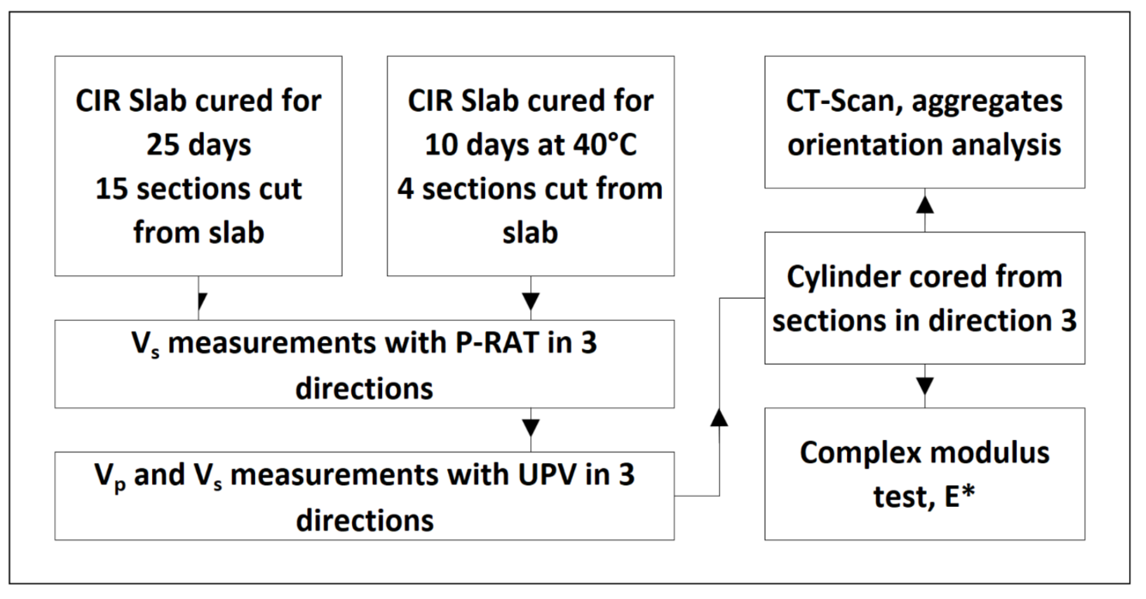
4. Materials and Methods

The study is composed of three different parts. The first part consists of V_s measurement in sections of a slab in three directions with the P-RAT and UPV techniques. The second part consists of conducting complex modulus tests on cylinders cored from these slab sections. Finally, the third part consists of performing CT scans on the same cylinders to evaluate the aggregates orientation. Figure 2 displays a schematic representation of the experimental campaign, with a detailed description of each part in the subsequent sections.

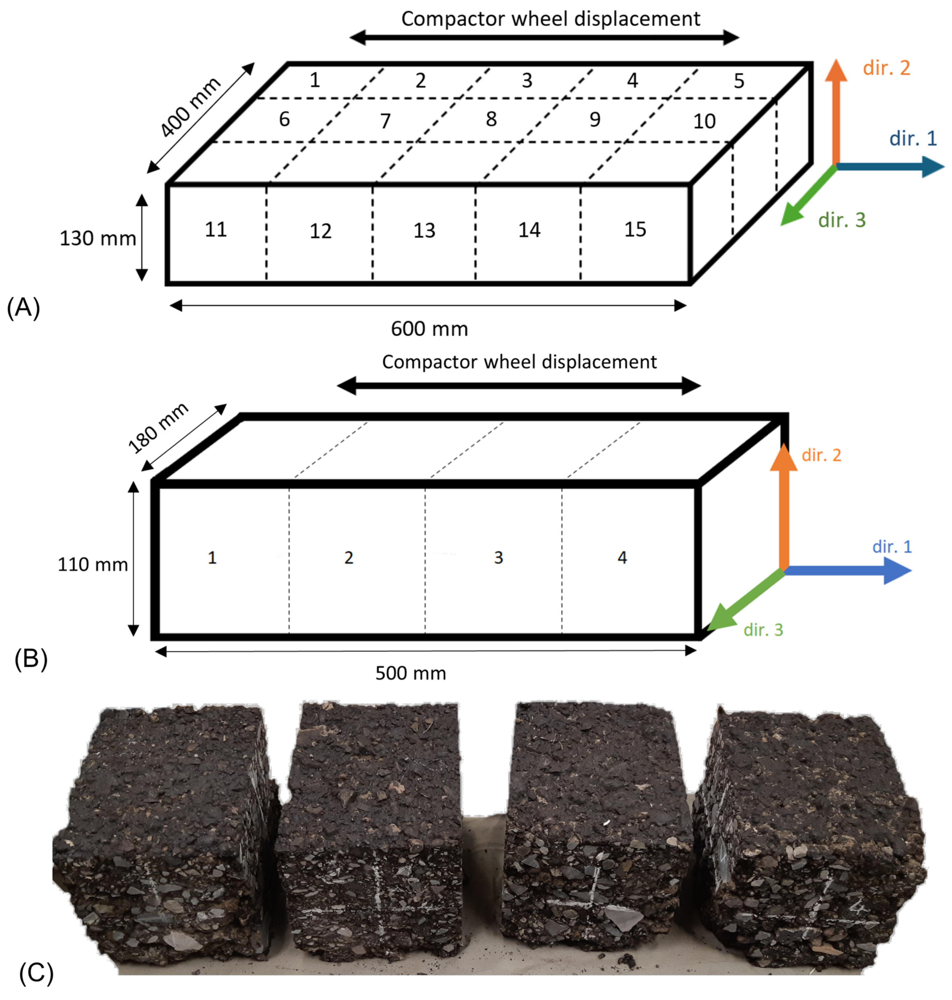
4.1. Materials Used and Specimens

The tested specimens are two CIR materials slabs. The first one is composed of 100% RAP material (0–10 mm) with 2% added bitumen in the form of asphalt emulsion, 6% added water, and 1% cement. The second slab is composed of 100% RAP material (0–20 mm) with 2% added bitumen in the form of asphalt emulsion (CSS-1, from McAsphalt, Toronto, ON, Canada) and 2% added water. All the mentioned percentages are related to the mass of RAP. The components were stored at room temperature and the RAP was not oven dried.

The slabs were compacted with a LPC French wheel compactor, following the procedure, although in the case of CIR materials, no metal wheel was used. The slab dimensions are 600 × 400 × 130 mm and 500 × 180 × 110 mm for slab 1 and slab 2, respectively. Slab 1 and slab 2 were cured in an oven at 40 °C for 25 and 10 days, respectively. After curing, the slabs were left in a freezer for 24 h to facilitate the cutting process. The slabs were cut in 15 sections of 105 × 105 × 130 mm and 4 sections of 110 × 140 × 110 mm blocs for slab 1 and slab 2, respectively. Figure 3A and Figure 3B present schematic views of slab 1 and slab 2, respectively.

The sections are referred to by the name of the slab and the number of the section, according to Figure 3. Section 4 from slab 2 is referred to as Slab2_4, for instance. Some sections were also covered with a bitumen mastic on each side to assess the improvement in contact and its influence on the P-RAT measurement. The bitumen mastic was made of ¼ bitumen (PG 58S-28) for ¾ sand (concrete sand), by mass.

Four cylinders of diameter 75 mm were cored from the sections of slab 2 in direction 3, as E* tests are usually performed with cylindrical specimens with a ½ diameter to length ratio. The four cylinders are designated specimens Slab2_1C to C_Slab2_4C, according to the section from which they were cored from.

Slab 1 was compacted to a targeted void ratio of 20%.

The bulk density was calculated according to LC-26-040 [39] by volumetric means due to the void ratio being larger than 10%. There is a lack of materials on the edge of the sections/cylinders due to cutting process. Therefore, the bulk densities are underestimated, and the resulting air void ratios are overestimated. The 3D analysis provides the air void ratio, without considering the edges of the specimens. The bulk density of specimen Slab2_2 to Slab2_4, their estimated void ratio, and calculated void ratio with 3D analysis are presented in

Table 1. Information on sections of slab 2.

Method	Specimen	Slab2_1C	Slab2_2C	Slab2_3C	Slab2_4C
LC 26-040	Volumetric bulk density (g·cm−3)	1.910	1.940	1.985	1.900
	Air void ratio (%)	24.1	22.9	21.1	24.5
Three-dimensional analysis	Air void ratio (%)	N.A.	17.2	16.5	17.1
	Calculated bulk density (g·cm−3)	N.A.	2.084	2.102	2.086

. Due to damages on specimen Slab2_1C, no 3D analysis was performed.

4.2. P-RAT Anisotropy Measurements

The tests were conducted uniformly across all tested sections. The objective of the study is to evaluate the anisotropic behavior of the CIR material. To this end, each block was tested in 3 different directions (dir. 1, dir. 2, and dir. 3), according to Figure 3.

Different pairs of transducers were used in this study. As shown in Lecuru et al. [33], the dimensions of the transducer do not influence the results significantly, although for smaller transducer size, wave diffraction can occur if the aggregate diameter exceeds the transducer wavelength [37]. Still, three main different transducer pairs were used in this study for control purposes and to ensure reproducibility. The designation of the transducers refers to the outer–inner diameter, namely 19–16 mm, 26–22 mm, and 36–31 mm. The inner stones of the transducers are made of four-quarter aluminum cylinders. Other transducers were used in the case of slab 1, mostly for testing newly made transducers or enhanced former transducers. Some of the transducers are encased in a plastic capsule, which mitigates the stress on the transducer during testing.

Transducers are positioned with care, ensuring that they are correctly aligned with one another. One transducer, acting as the emitter, is connected to a signal generator, Handyscope HS3 100 MHz (TiePie Engineering, Sneek, The Netherlands). The second transducer, acting as the receiver, is connected to another entry of the same apparatus, which also act as an oscilloscope. An amplifier, 7602M from Krohn-Hite (Brockton, MA, USA), is used on the generator side. The Handyscope is operated by a personal computer on which one can observe the emission and the reception signals. The form, amplitude, and frequency of the input signal are selected on the computer.

A single pair of transducers was used at a time, a rubber band was used to hold the transducer onto the specimens. Each pair was positioned in the same location, at the center of the surface. If the contact at this spot is insufficient to ensure optimal signal quality, the transducers are repositioned a few millimeters away. For repeatability and control concerns, signals of different shapes and frequencies are used when testing the specimen with a given transducer pair. To remove potential noise in an individual signal, the signals are sent eight times and stacked. Every specimen was tested at room temperature, and under the same conditions. A total of 1334 and 703 signals, without considering the stacking steps mentioned earlier, were collected for slab 1 and slab 2, respectively, considering all pairs of transducers used. Finally, these signals are then analyzed with a dedicated P-RAT software (version 2) developed in LabView (National Instruments, Austin, TX, USA) with the aforementioned concept obtained from Sherbrooke University [30].

4.3. UPV

The PUNDIT PL-200 device (ScreeningEagle, Zurich, Switzerland) is a device mainly employed in the monitoring of concrete materials via UPV. The Pundit device was used to monitor the P-wave and the S-wave in the tested specimens. To ensure good contact between the specimens and the sensors, coupling media was used as recommended by the PUNDIT supplier. The sensors used for the generation and reception of P-waves and S-waves have a resonant frequency of 54 and 250 kHz, respectively. Each sensor was manually held in place to ensure a sufficient contact with the tested specimen, and the sensors were kept aligned. The results have been analyzed in the Pundit software (PL-Link, version 3).

To obtain the S-wave flight time, one has to compare the received P-wave signal with the received S-wave. Indeed, even with a dedicated S-wave sensor, a weaker P-wave is generated. The following study investigates three different configurations regarding the arrival time of the received signal: first arrival, first peak, and second peak. There is no information on the nature of the input signal generated by the Pundit PL-200 device. Therefore, the flight time of either the P-wave or the S-wave is taken as shown in Figure 1, as instructed by the Pundit method.

4.4. Complex Modulus E*

The linear viscoelastic behavior of the cored cylinder was evaluated by dynamic tension–compression tests. Sinusoidal cyclic axial loads were applied with a hydraulic press (MTS) in a controlled deformation mode. The amplitude of the deformation was selected to be around 50 μm/m. The cylinders were glued to metallic caps using epoxy and equipped with three extensometers of 50 micrometer in the axial direction and temperature probes.

Specimens Slab2_3C and Slab2_4C were tested at 1, 0.3, 0.1, 0.03, and 0.01 Hz at 40, 30, 20, 10, 0, −10, and, −20 °C; and 25, 15, 5, −5, −15, −25, and −35 °C for specimen Slab2_3C and with the last array of temperature for Slab2_4C. The experimental results were analysed using the 2S2P1D model, which is a linear viscoelastic model composed of two springs, two parabolic elements, and one dashpot [9,10,11,40,41]. More details can be found in the mentioned references. The following equation is used to calculate the complex modulus E*:

$$E_{2S2P1D}^{\mathrm{*}}\left(\omega \right)=E_{00}+{\displaystyle \frac{E_0-E_{00}}{1+\delta {\left(j\omega {\tau }_E\right)}^{-k}+{\left(j\omega {\tau }_E\right)}^{-h}+{\left(j\omega \beta {\tau }_E\right)}^{-1}}}$$

(1)

where ω is the angular frequency; j is the imaginary unit; k, h, δ are constant (0 < k < h < 1); E₀₀ is the static modulus, when ω tends to 0; E₀ the glassy modulus, when ω tends to infinite; β, parameter linked with η, the dynamic viscosity of the dashpot, η = (E₀ − E₀₀) βτ_E; τ_E, the characteristic time values. The characteristic time values vary with the chosen temperature T and the shift factor a_T, τ_E(T) = a_T(T) × τ_0E.

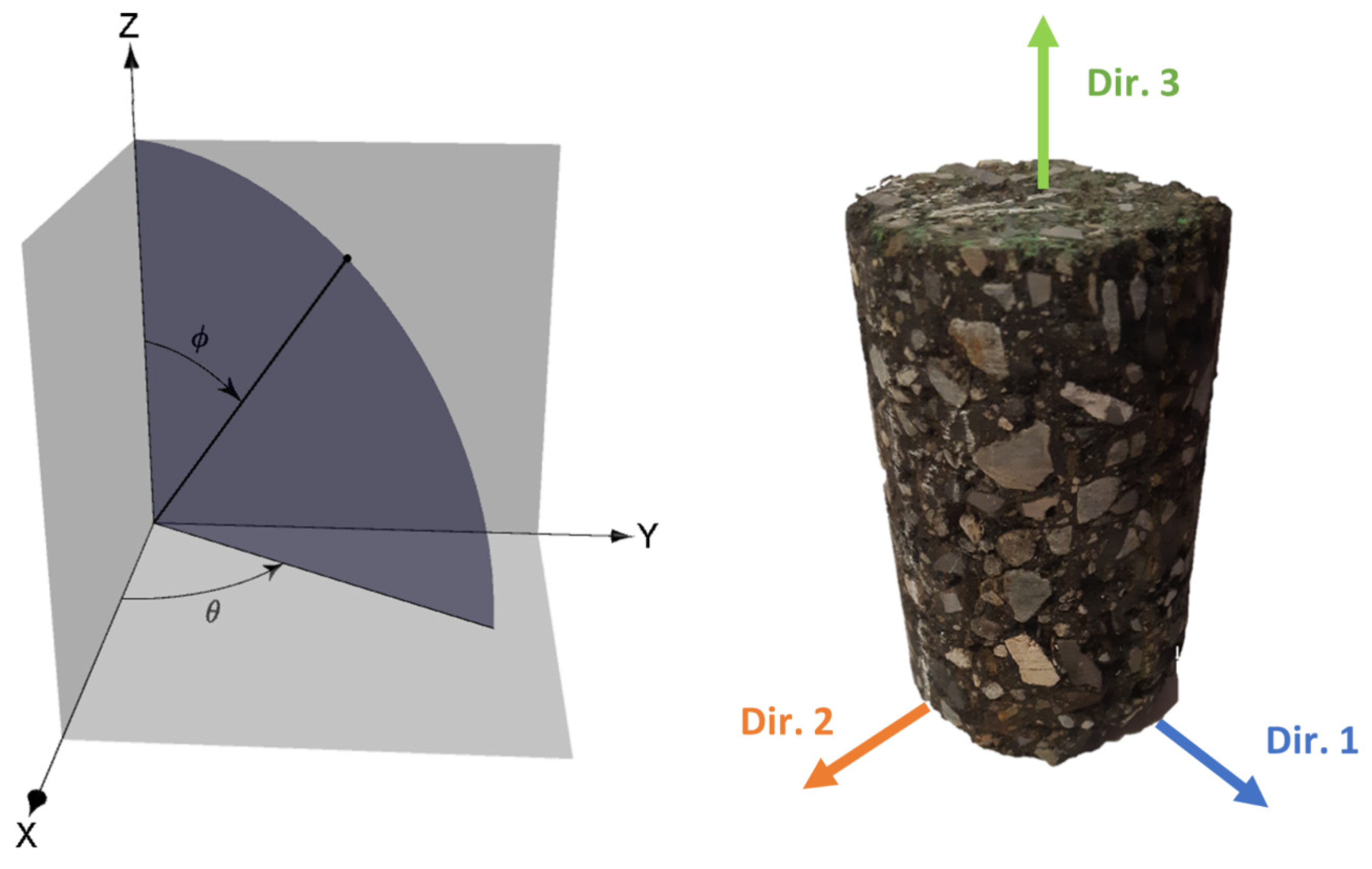
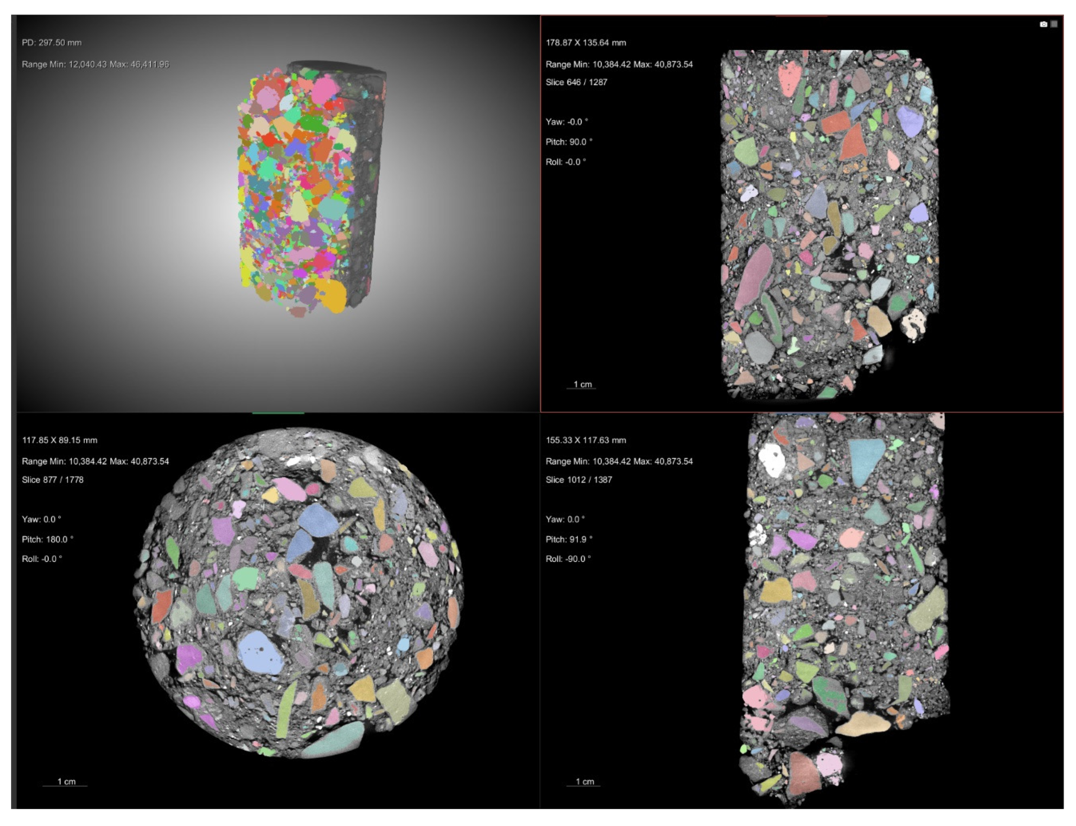
4.5. Computed Tomography Scan (CT-SCAN) and 3D Image Analysis

CT scans were performed to assess any specific particles orientation in the mix. The XTH-225 device from Nikon (Tokyo, Japan) was used for specimen Slab2_3C while a FF35 from Comet Yxlon was utilized for specimens Slab2_2C and Slab2_4C. CT scans were conducted with a voltage of 210 kV and a current of 210 μA for specimen Slab2_3C, and a voltage of 209 kV and a current of 108 μA for specimens Slab2_2C and Slab2_4C. Two distinct scanning devices were utilized for availability concerns. The 3D specimens were analysed with Dragonfly software, version 2023 (Comet Technologies Canada Inc., Montréal, QC, Canada). The cubic voxel size was 68.63 μm for specimen Slab2_3C and 30.75 μm for specimens Slab2_2C and Slab2_4C.

The 3D images data set size was first reduced to remove parts affected by artefacts, such as cone beam artefacts at the upper and lower parts of the data set. Then the data set was filtered to ease the segmentation process. Mainly, a smoothing filter was applied to reduce noise within the images, and a radial basis function (RBF) filter was used to mitigate greyscale variation across the images due to beam hardening and the cylindrical shape of the specimens. Granular materials were segmented and labelled individually with the tools offered by Dragonfly software, version 2023. During the segmentation process, some errors can be introduced, mostly due to the spatial and the contrast resolution of the voxels. For instance, a voxel can be labelled as “aggregate” though it could be “bitumen mastic”. But, in the present study, it does not impact the aggregate orientation as aggregates composed of few voxels were not considered in the final analysis.

The orientation of the longest axis of a labelled particle was evaluated with 2 parameters, Φ and θ angles, θ being the angle between the X axis and the projection of the longest axis in the X–Y plane; and Φ the angle between the longest axis and Z axis, as shown in Figure 4.

Air voids were also segmented, in order to calculate the air void ratio of the tested specimens by comparing the labeled void voxel to the global voxel count. A contrast-limited adaptive histogram equalization (CLAHE) filter was applied to enhance the contrast in the data set, when required.

5. Results and Analysis

In this section, the results concerning anisotropy are presented first. V_s results obtained with the P-RAT in the slabs are analysed and the particles orientation of aggregates is presented. UPV results are discussed. Afterward, the results of the complex modulus are presented, and a comparison with wave velocities is made.

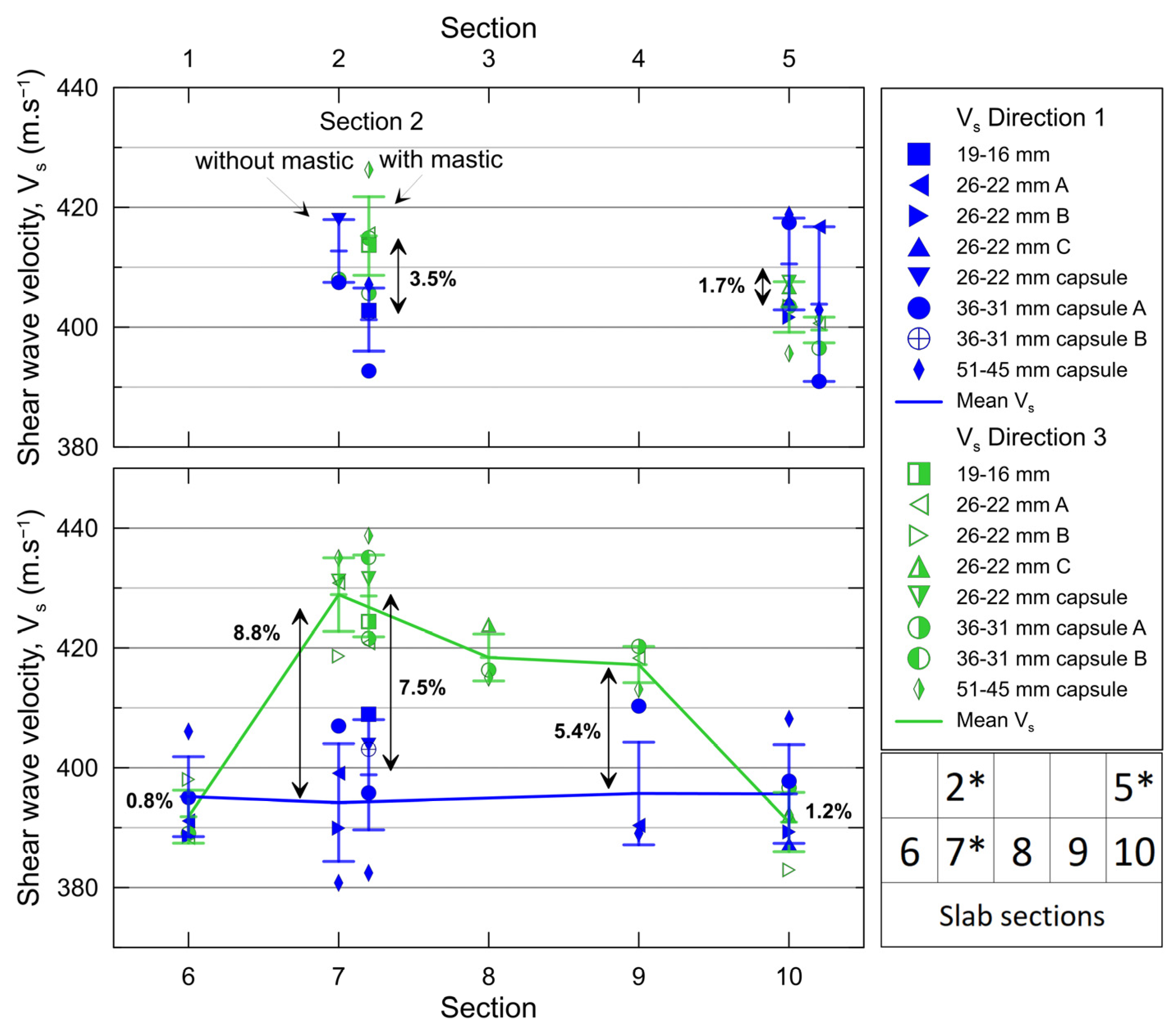
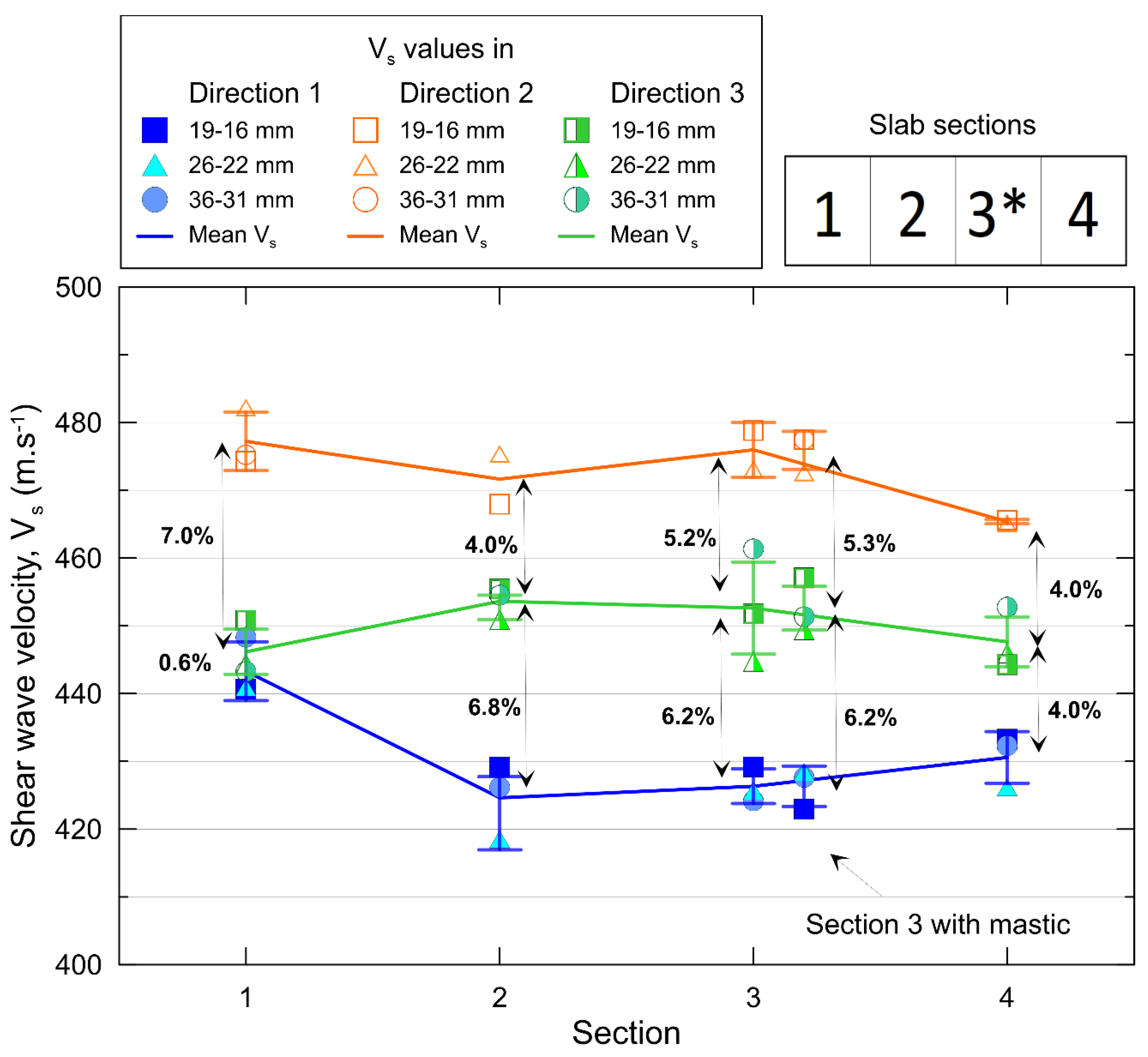
5.1. P-RAT Shear Wave Velocity (V_s) Results

Figure 5 illustrates the effects of bitumen mastic on two signals. In both cases, the presence of a P-wave is observed, but it is more pronounced in the case of the mastic interface. However, the signal is clearer. The P-RAT transducers are designed to generate mainly shear waves. Due to the size of the specimen and the quality of the contact, in order to obtain a signal at the receiver end, it is sometimes necessary to amplify the emitted signal, generating larger deformation of the piezoelectric ring. Such amplification tends to generate more P-wave. It has been observed that in the case of the bitumen interface, the P-wave amplitude is higher than the S-wave one compared to the case without mastic. The arrival times of the wave, calculated from the P-RAT V_s measurement are 0.294 and 0.309 ms for the signals with and without bitumen mastic, respectively. Figure 5C,D display an example of the P-RAT analysis. See Karray et al. [30] for more details.

The difference between V_s values in section Slab2_3 with and without mastic is 1.5, 2.7, and 1.3% for directions 1, 2, and 3, respectively. It was more convenient to lay the same thickness of mastic on the ends of Section 3 in directions 1 and 3 (2 mm on each face) than in direction 2. Indeed, the upper part surface of the slab is uneven, resulting in a thicker layer of mastic. This explains the higher difference observed in direction 2. P-RAT testing with various pairs of transducers have demonstrated that the mastic used to improve the interface gives V_s values of approximately 300 m·s⁻¹. In the case of a mastic interface, the S-wave propagates slower in the mastic layer, reducing the overall V_s. The actual V_s of the specimen can be calculated as the thickness of the mastic layer and the V_s values of the mastic used are known. In the following Figures, V_s depicted as “with mastic” display the corrected V_s values.

Regarding slab 2, for direction 2, only section Slab2_1 was monitored with the 36–31 mm transducer pair. The surface of the three other sections were too rough to allow for a proper contact of this larger size of transducer. The same situation occurred for specimens of Slab 1, preventing the acquisition of V_s results in its direction 2. V_s measurements in the tested section of slab 1 and in the four sections of the slab 2 are presented in Figure 6 and Figure 7, respectively. Each point represents the mean value of all measured signals. As mentioned in the P-RAT measurement section, several signals of various shapes and frequencies were sent for repeatability and control issues. For example, “V_s values in Direction 1 19–16 mm” is the mean value of all five treated signals (after stacking) for the 19–16 mm transducer pair in direction 1.

To simplify the text, V_s values for directions 1, 2, and 3 are referred to as V_s1, V_s2, and V_s3 respectively.

Table 2. Minimal V_s values, maximal V_s values, and relative standard deviation (σ%) for the pairs of transducers in slab 1.

Section	Vs1 (m·s−1)			Vs3 (m·s−1)
	Min.	Max.	σ%	Min	Max	σ%
Slab1_2	407.5	417.9	1.8%	408.0	408.0	N.A.
Slab1_2 mastic	388.4	401.9	1.4%	401.4	420.9	1.7%
Slab1_5	401.6	418.8	2.1%	395.6	407.4	1.2%
Slab1_5 mastic	387.2	411.7	3.1%	393.8	398.5	0.6%
Slab1_6	388.5	406.0	1.9%	388.4	398.1	1.4%
Slab1_7	380.8	406.9	2.9%	418.6	435.0	1.6%
Slab1_7 mastic	378.9	403.9	2.5%	415.8	432.7	1.7%
Slab1_8	N.A.	N.A.	N.A.	415.0	423.9	1.1%
Slab1_9	389.0	410.3	2.5%	413.1	420.3	0.9%
Slab1_10	387.3	408.2	2.4%	383.0	396.6	1.5%

and

Table 3. Mean V_s values and relative standard deviation (σ%) among the three pairs of transducers in slab 2.

Section	Vs1 (m·s−1)			Vs2 (m·s−1)			Vs3 (m·s−1)
	19–16	26–22	36–31	19–16	26–22	36–31	19–16	26–22	36–31
Slab2_1	440.7	440.9	448.3	474.3	482.2	475.2	450.8	444.5	443.2
σ%			1.0%	σ%		0.9%	σ%		0.9%
Slab2_2	429.1	418.5	426.2	467.9	475.4	N.A.	455.4	450.9	454.5
σ%			1.3%	σ%		1.1%	σ%		0.5%
Slab2_3	429.2	425.6	424.2	478.8	473.1	N.A.	451.8	444.8	461.3
σ%			0.6%	σ%		0.8%	σ%		1.8%
Slab2_3 mastic	417.0	422.2	421.4	465.6	461.2	465.6	450.3	443.2	445.0
	σ%		0.7%	σ%		0.5%	σ%		0.8%
Slab2_4	433.2	426.2	432.3	465.6	465.1	N.A.	444.3	446.0	452.8
σ%			0.9%	σ%		0.1%	σ%		1.0%

presents the relative standard deviation between the pairs of transducers for a single direction in the same section for slab 1 and slab 2, respectively. The maximum standard deviation in regard to the mean V_s values are 3.1 and 1.8% in slab 1 and slab 2, respectively. In a previous study, the mean standard deviation among different pair of transducers was approximately 2% [34]. It shows good reproducibility of the measure. More transducer pairs were utilized to evaluate V_s in slab 1’s sections, which explains the higher standard deviation in slab 1 compared to slab 2. As mentioned in Lecuru et al. [33], the different sizes of actuators do not influence significantly the values, as shown by the low differences presented in Table 2 and Table 3. Naji et al. [37] showed that the size of aggregates can generate wave diffraction, depending on the size of the P-RAT transducer used. Wave diffraction influences the propagation of shear waves in the tested specimen, therefore, it influences the shear wave velocity. The results obtained herein using transducers of various dimensions do not demonstrate systematically higher or lower values of V_s, depending on the dimension of the transducer, compared with the average values.

A trend emerges from the curves of Figure 6 and Figure 7. Especially away from the end of the slabs, V_s2 values are systematically greater than V_s3 and V_s1, and V_s3 is greater than V_s1.

In Figure 6, there is an axial symmetry relative to the middle tendency in the V_s values for sections Slab1_6–Slab1_7 and Slab1_9–Slab1_10. The same symmetry is observed in Figure 7, in V_s values for sections Slab2_2 and Slab2_3, and somewhat for sections Slab2_1 and Slab2_4. It is expected, as the tested specimens are pieces of a slab, that section Slab2_2 and Slab2_3 should be compacted in the same state, as should section Slab2_1 and Slab2_4.

V_s1 and V_s3 are higher in Slab1_5 than in Slab1_10. This may be because Slab1_5 is located at the corner of the sample. V_s1 is higher in Slab1_2 and Slab1_5 than in Slab1_6 to 10. Slab1_1 to 5 are along the side of the sample. It can be assumed that the edges of the mold create a confinement in the materials during compaction. The confinement might induce a better aggregate contact, resulting in a higher V_s value. This confinement is greater in direction 3 than in direction 1, due to the dimension of the mold, which is smaller in direction 3 than in direction 1. This confinement becomes more homogeneous in sections Slab2_1, Slab2_4, and Slab1_5, which explains the closeness of V_s1 and V_s3 values in these sections.

The difference between V_s1 and V_s3 values could also be explained by the nature of the S-waves and the way the slabs are compacted. The compacting wheel moves in direction 1 and, therefore, the aggregates tend to move along. This movement can result in friction between the aggregate in a perpendicular direction, i.e., direction 3. In S-waves, the local displacement of matter is perpendicular to the direction of wave propagation.

The relative differences between mean V_s values in the different direction are presented in Figure 6 and Figure 7. Concerning slab 2, the maximum relative differences are 7.6, 11.1, 11.6, and 8.1% for sections Slab2_1, Slab2_2, Slab2_3, and Slab2_4, respectively. In order to compare these values with the literature, Equation (2) is used to estimate the equivalent modulus [22]:

$$V_s={\displaystyle \frac{1}{\cos \left(\frac{\phi }{2}\right)}}\sqrt{{\displaystyle \frac{\left|E^{\mathrm{*}}\right|}{2\rho \left(1+\nu \right)}}}$$

(2)

With the phase angle ϕ, the bulk density ρ (kg·m⁻³), the Poisson ratio ν, V_s the shear wave velocity (m·s⁻¹), and E* the complex modulus (Pa).

The maximum relative differences in modulus for the aforementioned specimens are 15.9, 23.4, 24.6, and 16.8%, respectively. The relative differences values observed in the literature for HMA range from 10 to 50% [10,11,42]. As explained earlier, the anisotropy is influenced by many parameters, which explains the wide array of values in the literature.

The maximum value always appears between V_s2 and V_s1, and the symmetric trend is respected. Although no analysis of variance was performed, it can be assumed that the V_s values in the three directions are different in each section, except for V_s1 and V_s3 in sections Slab2_1, Slab1_5, Slab1_6, and Slab1_10. The symmetry of the results demonstrates the consistency of the results, and the systematic differences observed implies anisotropy in the tested CIR.

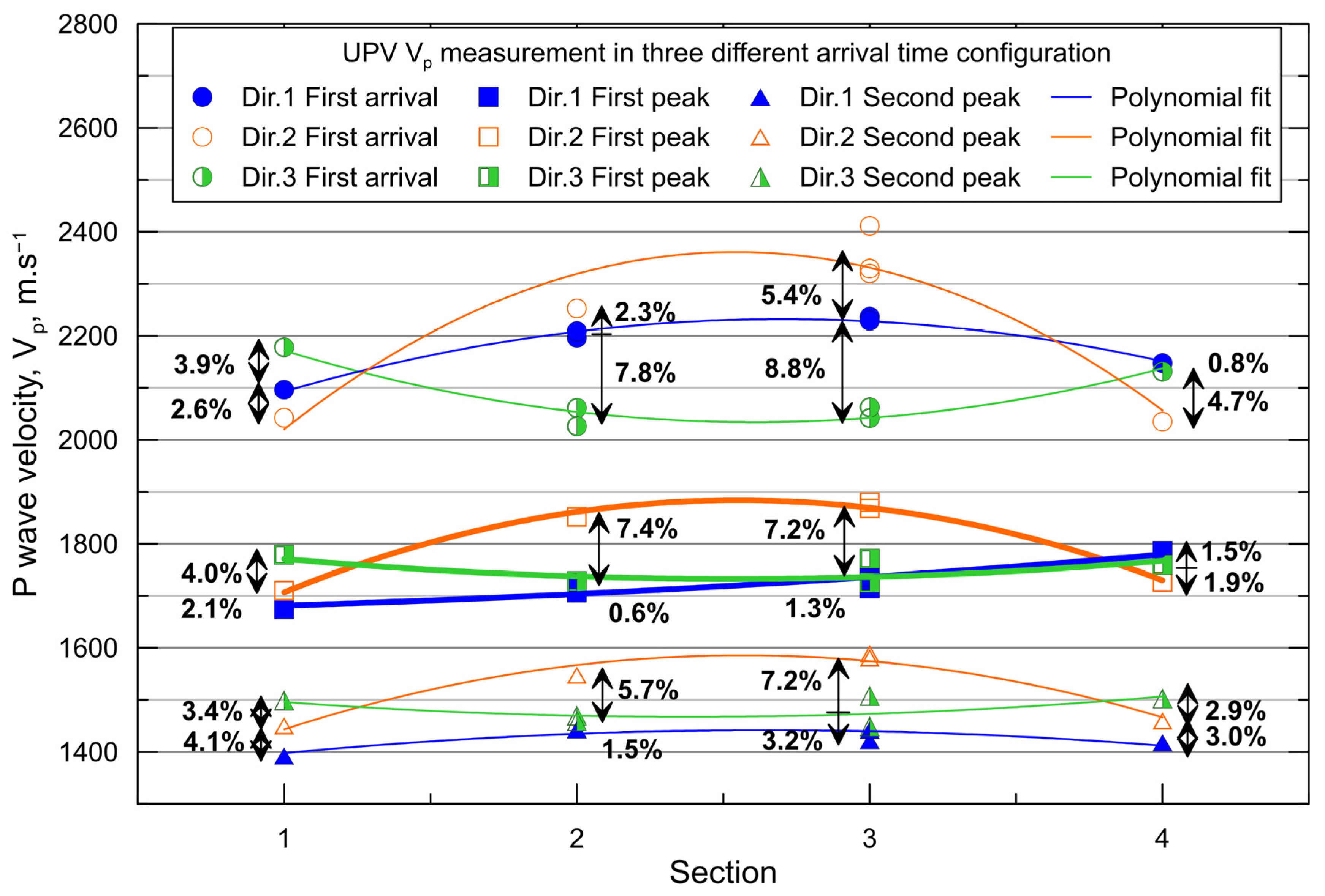
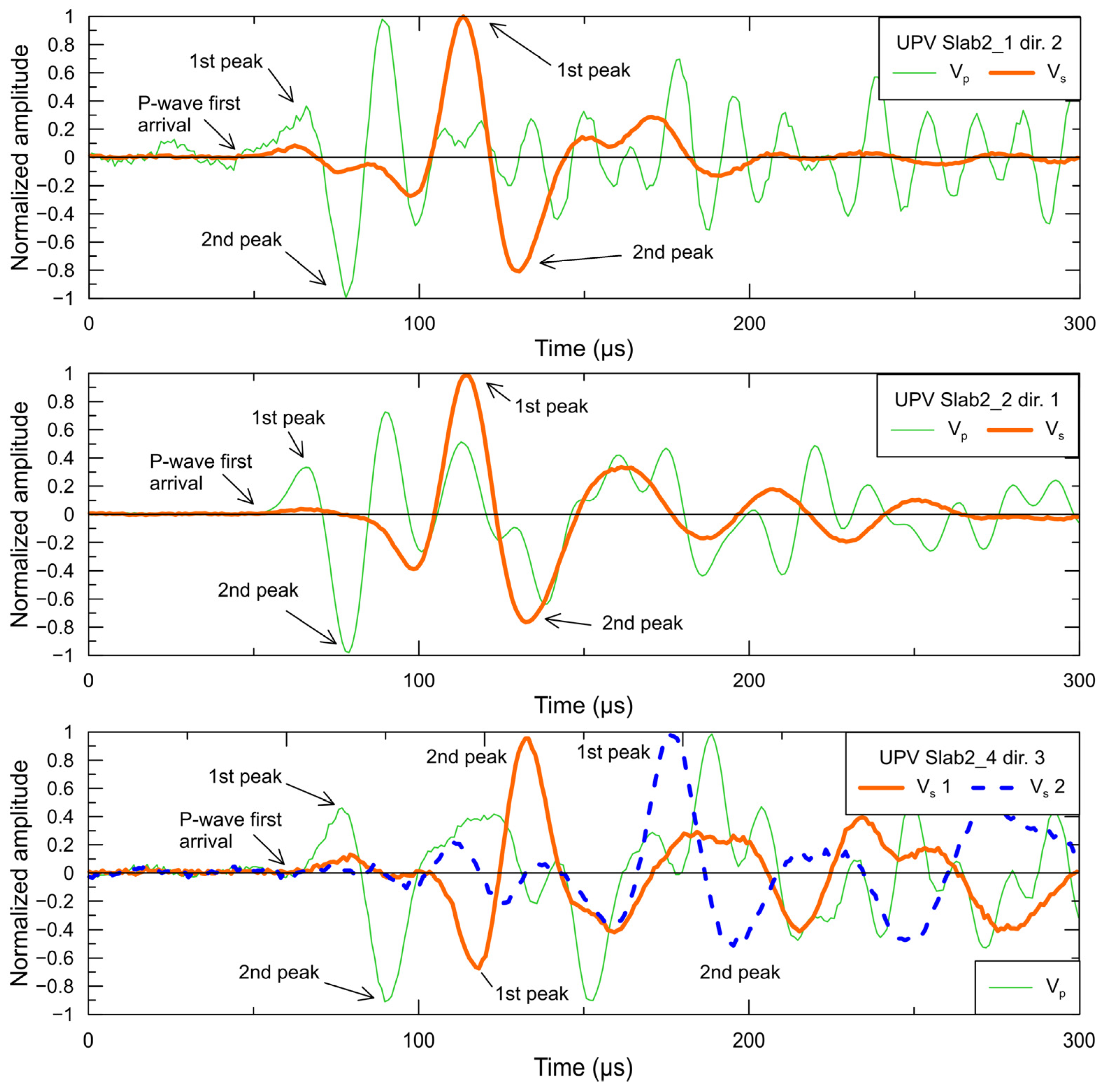
5.2. UPV Test Results

The results of UPV tests are presented in Figure 8 for the P-wave. Although the choice of arrival time configuration is not obvious, the first peak (bold line in Figure 8) tends to depict a similar behavior to what is observed in P-RAT test results (Figure 7). A trend emerges among the sections monitored with P-wave. The axial symmetry relative to the middle observed for P-RAT analysis occurs here as well. For sections Slab2_2 and Slab2_3 (i.e., in the middle of the slab), V_p in dir. 2 is higher than in the other two directions. The opposite happens in sections Slab2_1 and Slab2_4. The relative difference between V_p values in a same section are displayed in Figure 8. The difference between V_p values can reach up to 12.8% in the case of section Slab2_3. The relative differences are lower in sections Slab2_1 and Slab2_4, for every arrival time setup. This reduction in relative difference between the edges of the slab and the inner parts was also observed in V_s values obtained with P-RAT. The boundaries conditions applied by the metallic mold in the outer sections of the slab may impact the compaction of the mix and may cause anisotropy.

The analysis of the UPV S-wave is more difficult. As mentioned earlier, to obtain the S-wave flight time, one must compare the received P-wave signal with the received S-wave. In the tested sections, the distinction between the P-wave and the S-wave was not readily apparent, and this can can lead to erroneous assumptions regarding the location of the first and second peaks. It was almost impossible to determine where the first arrival of the S-wave was. Figure 9 presents examples of P- and S-wave signals to illustrate the difficulties mentioned before. In the case of section Slab2_4 in direction 3, two different S-wave signals give different results. Due to these erratic results, and their inconstancy even for a same specimen in the same direction, S-wave UPV results are reported as Supplementary Materials.

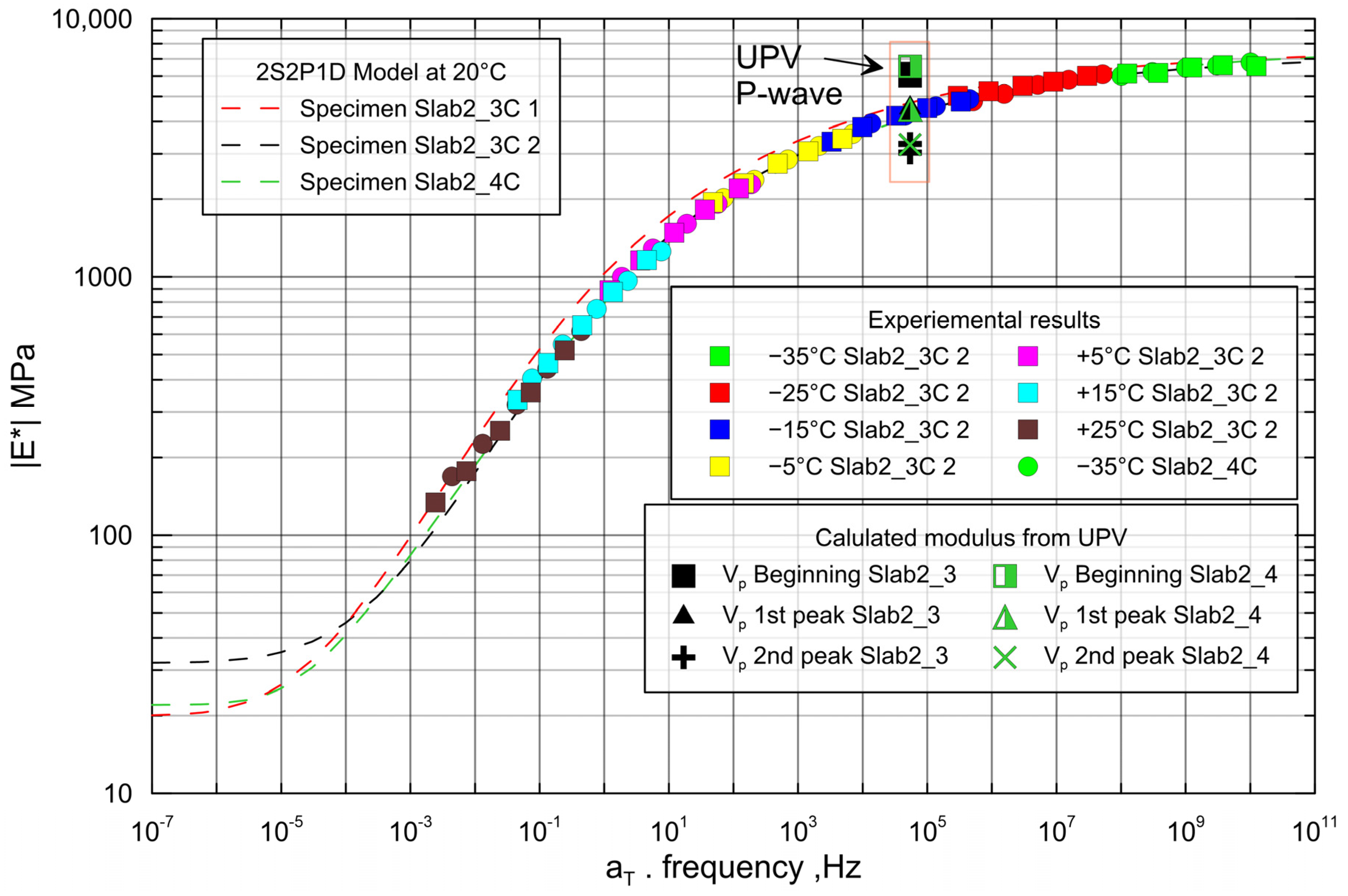
5.3. Complex Modulus

This section presents the results of the complex modulus measurements. It should be noted that specimen Slab2_3C has been tested twice. The master curves of specimens Slab2_3C 1 and 2 and Slab2_4C are plotted in Figure 10.

Table 4. The 2S2P1D parameters.

	E00	E0	ν00	ν0	k	H	δ	τ	β	C1	C2
	MPa	MPa						(Tref)
Slab2_3C 1	20	7500	/	/	0.170	0.475	2.56	0.2 (10.93)	5000	20.00	159.12
Slab2_3C 2	32	7200	/	/	0.170	0.490	2.69	1.1 (4.96)	5000	24.02	158.55
Slab2_4C	22	7675	/	/	0.161	0.450	2.85	1.1 (4.96)	5000	23.47	159.08

compiles the 2S2P1D parameter used for the analysis of the experimental results.

The specimens were equipped with a chain to measure radial deformations, but the results obtained were erratic and did not follow the usual trends that appear in the literature. It is assumed that the applied strain was too small to obtain enough amplitude in the transverse direction. The strain measured by the chain was mainly noise, rather than actual displacement. The results are not presented for this reason.

It appears that there is a reduction in the modulus for specimen Slab2_3C when performing the second tension–compression test. Although the strain amplitude was small, some damage can be induced to the specimen.

The results from UPV testing were converted into modulus, with the following equation [22]:

$$V_p={\displaystyle \frac{1}{\cos \left(\frac{\phi }{2}\right)}}\sqrt{{\displaystyle \frac{\left|E^{*}\right|(1-\nu )}{\rho \left(1+\nu \right)(1-2\nu )}}}$$

(3)

and considering the following parameters: the phase angle ϕ = 20° (from E* tests), the bulk density ρ = 2000 kg·m⁻³ (from measurement), and the Poisson ratio ν = 0.3 (assumed). Their |E*| moduli are plotted along the master curve, at a reference temperature of 20 °C, considering the frequency of the UPV sensor used, 50 kHz for P-wave. The moduli for the different arrival time setups, i.e., first arrival of the signal, first peak, and second peak (see Figure 1) are plotted. The relative differences between the experimental |E*| modulus and the UPV modulus calculated from the aforementioned arrival time configurations are 35, 2, and 30%. It appears that the first peak arrival time configuration of P-wave fits the master curve.

Mounier et al. [22] and Larcher et al. [26] observed differences between the UPV modulus and 2S2P1D model, considering the arrival of the wave at the first arrival of the signal, from 5 up to 30% and 12%, respectively. Both studies point out the importance of accuracy in measuring the arrival time of the wave.

Mean P-RAT V_s values in dir. 3 for Section 3 and 4 are 452.6 and 447.7 m·s⁻¹, respectively. Their equivalent |E*| modulus considering ϕ = 20°, ν = 0.3, and ρ presented in Table 1 are 1057 and 990 MPa for sections Slab2_3 and Slab2_4, respectively. These moduli come from a group shear wave velocity and, therefore, are not bound to frequency. Therefore, these moduli cannot be plotted in the master curve. In a previous study by Lecuru et al. [34], moduli calculated from V_s results obtained with P-RAT tests were compared with indirect tensile strength modulus (ITSM) test results. They demonstrated consistency, for a similar CRM mix.

For V_p, the first peak arrival time configuration appears to be the one to consider. It was mentioned earlier that V_p results obtained with this particular configuration show a similar trend to the one observed for P-RAT V_s results. This gives greater confidence regarding anisotropic results in the mix.

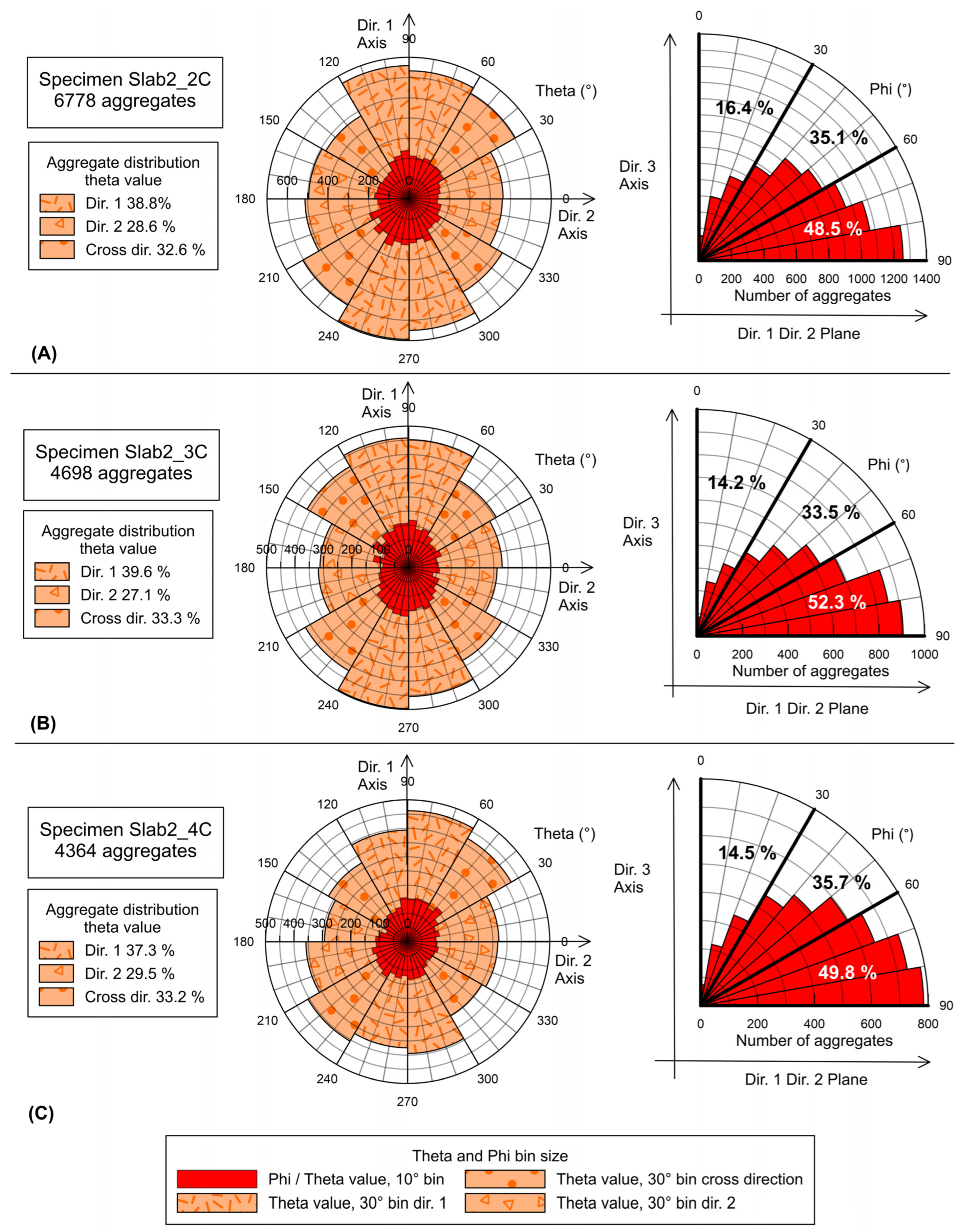
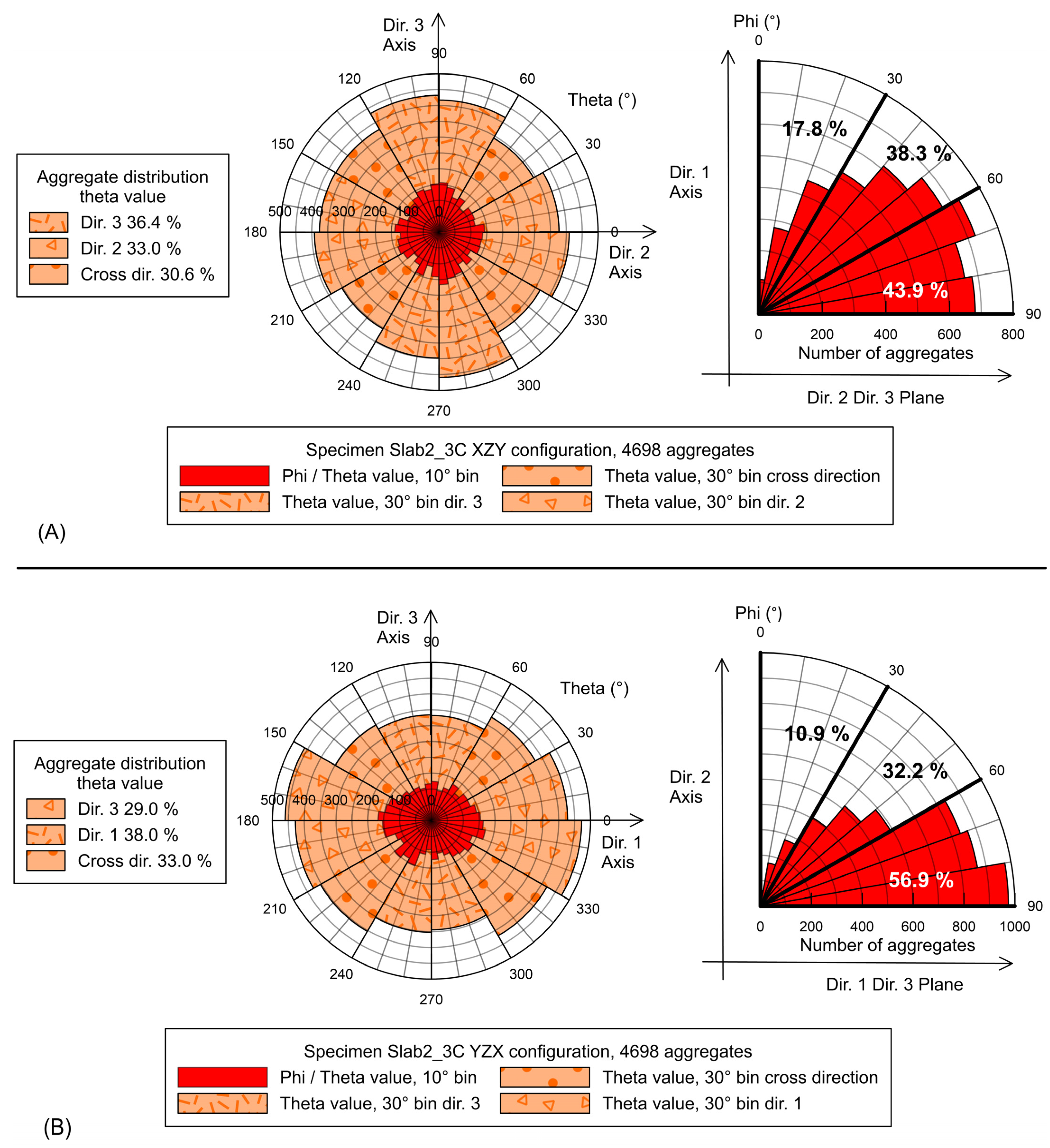
5.4. Three-Dimensional Image Analysis Results

For the analysis of the 3D images, the particles were segmented and then individually labelled, as shown in Figure 11. Among all labelled particles, any larger than 1 mm³ were selected for analysis according to the Dragonfly analysis, corresponding to 6778, 4698, and 4364 particles in specimen Slab2_2C, Slab2_3C, and Slab2_4C, respectively. It appears that smaller labelled particles tend to be spherical, and the analysis attributes arbitrary values of phi and theta angle of 0° or 90° to them. Specimen Slab2_1C was destroyed during a tension compression test and was not scanned.

Figure 12A–C presents the results of the angular orientation analysis for specimens Slab2_2C, Slab_3C, and Slab2_4C, respectively. The axis systems in Figure 12 are the same as that presented in Figure 3.

In each specimen, the particles tend to be oriented in the dir. 1 dir. 2 plane rather than the dir. 3 axis (phi values) as 48.4, 52.3, and 49.8% of the aggregates are enclosed in the 60 to 90° range for specimens Slab2_2C, Slab2_3C, and Slab2_4C, respectively.

For the theta analysis, i.e., the orientation in the dir. 1 dir. 2 plan, three sets of data are considered and are represented in Figure 12A–C. The aggregates aligned with dir. 1 are enclosed in the bins from 60 to 120° plus 240 to 300° (orange dashes); the aggregates aligned with dir. 2 are enclosed in the bins from 330 to 30° plus 150 to 210° (orange triangles); the rest are considered as the cross direction (orange dots).

For each specimen, the aggregates tend to be more oriented in dir. 1 than in dir. 2. As the compactor wheel is moving along the dir. 1 axis, it is expected that aggregates would be more aligned in this direction. However, a non-negligible part of the aggregates is aligned in the dir. 2 axis and in a cross direction of dir. 1 and dir. 2 axes.

The phi and theta angles are bound to the axis system of the Dragonfly software. An axis swap enables the user to evaluate the orientation of aggregates from different perspectives. Figure 13 presents the results of phi and theta angle analysis in, according to Dragonfly, the XZY (Y and Z axis swapped) and YZX configuration. The default configuration (XYZ) is presented in Figure 12B.

In Figure 12B, the particles tend to be oriented in the dir. 1 dir. 2 plane rather than dir. 3 (phi values) and more aligned in dir. 1 (theta values). In Figure 13, view (A), the particular orientation is not as straightforward. Considering the phi values, more aggregates are enclosed in the 30° to 60° area and less in the 60° to 90° area, compared to views (A) and (C). There is a slight increase in the 0° to 30° area, but not as much as expected if we consider a preferential orientation of the aggregates in dir. 1. Regarding the theta values, there is no particular orientation in dir. 2, dir. 3, nor in the cross direction. In Figure 13, view (B), particles tend to be oriented in the dir. 1 dir. 3 plane rather than dir. 2 and more aligned in dir. 1.

Displaying 3D orientation in a 2D representation has always been challenging. However, the results indicate that the aggregates in the three tested specimens tend to be aligned in dir. 1, which corresponds to the direction of the compacting wheel. However, the different points of view for specimen Slab2_3C confirm that a non-negligeable portion of the aggregates are aligned in dir. 2 and dir. 3. This preferential orientation shows that compaction has induced anisotropy in the tested CIR.

In the case of clays, V_s is higher when propagating in the direction of the main axis orientation of particles [13,43]. The same phenomenon can be observed in granular materials such as micas [12]. This is the result of inherent anisotropy. However, clays and micas are characterized by their flat and elongated geometry, which is not the case of the aggregates composing a CIR mix.

In the case of the tested CIR, V_s is higher in dir. 2, followed by dir. 3, then dir. 1. Although the preferential orientation tends to be in dir. 1, V_s1 is the smallest. It can be assumed that compaction induces inherent anisotropy and that induced anisotropy, as defined in the background section, is not relevant in the case of wave propagation where strains are small [14,15,17], although the compaction generates some confinement due to the edges of the mold, which then become the inherent (natural) state of the material after unmolding. Wave propagation is, as mentioned earlier, impacted by the orientation of particles, but also by the contacts between them. However, in HMA and CIR mixes, the bitumen mastic plays a role in the stiffness of the material and, therefore, the alignment of aggregate alone is not sufficient to fully understand the differences in the measured V_s in the three directions. Finally, the air voids orientation and distribution could also provide useful information, although it has not been evaluated in this study.

6. Conclusions

A non-destructive method using shear wave velocity was used in the study. The P-RAT was used to measure V_s in the three directions of a CIR slab cut in sections. For comparison purposes, UPV measurements were also performed. Cylinders cored from the section in direction 3 were tested by dynamic tension–compression test to evaluate the complex modulus. Finally, CT scans were performed on the cylinders to evaluate the orientation of the aggregates. Anisotropy was witnessed for both approaches.

• V_s measurements with P-RAT show a systematic anisotropy in the two tested slabs. Different sizes of P-RAT transducers were used and the variability was low. V_s in the direction of compaction is higher than V_s in the orthogonal direction of displacement of the compacting wheel, which is higher than V_s in the direction of the compacting wheel; V_s2 > V_s3 > V_s1. Differences between V_s values range from 0.6 to 11.6%. V_s values on the outer sections of the slabs tend to be closer to one another compared to the middle section. The difference in wave velocities is explained by the compaction method and the dimensions of the mold, which generate uneven confinement in the mix.
• UPV results with PUNDIT also show anisotropy. UPV V_p values are different in every direction, and the same axial symmetry relative to the middle of the slab was observed as in P-RAT results. V_s values from UPV were trickier to obtain, as the arrival time of the wave is hard to determine. Various setups of arrival time were then tested. V_s from P-RAT and V_p from UPV results are consistent one with each other.
• E* results are consistent in the tested specimens, and they were modelized with the 2S2P1D model. Moduli from UPV were plotted in the master curve and the proper arrival time setup were determined to be the first peak for P-wave.
• CT scans highlighted a preferential orientation of the aggregate in the direction of the movement of the compacting wheel, dir. 1. However, a non-negligible part of the aggregates is oriented in the two other directions.

This study was focused on a two CIR mixes with a single method of compaction due to the high quantity of signal collected. Future work should focus on determining the influence of the degree of compaction as well as the method of compaction, such as SGC and slab compactor, on the anisotropy of CIR materials. V_s measurements would benefit from the analysis of contacts between aggregates. Finally, the evaluation of the anisotropy in CIR mixes while curing and in the long term could be achieved with the P-RAT and V_s.

References

1. Raschia, S.; Perraton, D.; Graziani, A.; Carter, A. Influence of low production temperatures on compactability and mechanical properties of cold recycled mixtures. Constr. Build. Mater. 2020, 232, 117169. [Google Scholar] [CrossRef]
2. Sangiorgi, C.; Tataranni, P.; Simone, A.; Vignali, V.; Lantieri, C.; Dondi, G. A laboratory and filed evaluation of Cold Recycled Mixture for base layer entirely made with Reclaimed Asphalt Pavement. Constr. Build. Mater. 2017, 138, 232–239. [Google Scholar] [CrossRef]
3. Orosa, P.; Orozco, G.; Carret, J.C.; Carter, A.; Pasadín, A.R. Compactablility and mechanical properties of cold recycled mixes prepared with different nominal maximum sizes of RAP. Constr. Build. Mater. 2022, 339, 127689. [Google Scholar] [CrossRef]
4. Li, Y.; Lyv, Y.; Fang, L.; Zhang, Y. Effects of Cement and Emulsified Asphalt on Properties of Mastics and 100% Cold Recycled Asphalt Mixtures. Materials 2019, 12, 754. [Google Scholar] [CrossRef]
5. Kuchiishi, A.K.; Vasconcelos, K.; Bernucci, L.L.B. Effect of mixture composition on the mechanical behavior of cold recycled asphalt mixtures. Int. J. Pavement Eng. 2021, 22, 984–994. [Google Scholar] [CrossRef]
6. Raschia, S.; Graziani, A.; Carter, A.; Perraton, D. Laboratory mechanical characterization of cold recycled mixtures produced with different RAP sources. Road Mater. Pavement Des. 2019, 20, 233–246. [Google Scholar] [CrossRef]
7. Diefenderfer, B.K.; Bowers, B.F.; Shwartz, C.W.; Farzaneh, A.; Zhang, Z. Dynamic Modulus of Recycled Pavement Mixtures. J. Transp. Res. Board 2016, 2575, 19–26. [Google Scholar] [CrossRef]
8. Nguyen, L.N.; Nguyen, M.H.; Dao, D.V.; Nguyen, P.Q.; Nguyen, T.M.T.; Tran, T.D. Effect of curing regimes on the dynamic modulus of entirely RAP cold recycled asphalt mixture. J. Mater. Des. Appl. 2023, 237, 1975–1989. [Google Scholar] [CrossRef]
9. Pham, N.H.; Sauzéat, C.; Di Benedetto, H.; González-Leön, J.A.; Barreto, G.; Nicolaï, A.; Jakibowski, M. Analysis and modeling of 3D complex modulus tests on hot and warm bituminous mixtures. Mech. Time-Depend Mater. 2015, 19, 167–186. [Google Scholar] [CrossRef]
10. Di Benedetto, H.; Sauzéat, C.; Clec’h, P. Anisotropy of bituminous in the linear viscoelastic domain. Mech. Time-Depend Mater. 2016, 20, 281–297. [Google Scholar] [CrossRef]
11. Nguyen, Q.T.; Pham, N.H.; Di Benedetto, H.; Sauzéat, C. Anisotropic Behavior of Bituminous Mixtures in Road Pavement Structures. J. Test. Eval. 2020, 48, 178–188. [Google Scholar] [CrossRef]
12. Santamarina, J.C.; Klein, K.A.; Fam, M.A. Soils and Waves: Particulate Materials Behavior, Characterization and Process Monitoring, 1st ed.; John Wiley & Sons Ltd.: Chichester, UK, 2001; ISBN 0-471-49058-X. [Google Scholar]
13. Nguyen, T.L.; Szymkiewicz, F.; Reiffsteck, P.; Bourgeois, E.; Mestat, P. Caractérisation et effet de l’anisotropie sur le comportement de sols reconstitués. Rev. Can. De Géotechnique 2011, 48, 1520–1536. [Google Scholar] [CrossRef]
14. Massad, E.; Tashman, L.; Somedavan, N.; Little, D. Micromechanics-Based Analysis of Stiffness Anisotropy in Asphalt Mixtures. J. Mater. Civ. Eng. 2002, 14, 374–383. [Google Scholar] [CrossRef]
15. Underwood, S.; Heidari, A.H.; Guddati, M.; Kim, R. Experimental Investigation of Anisotropy in Asphalt Concrete. J. Transp. 2005, 1929, 238–247. [Google Scholar] [CrossRef]
16. Bhasin, A.; Izadi, A.; Bedgaker, S. Three dimensional distribution of the mastic in asphalt composites. Constr. Build. Mater. 2011, 25, 4079–4087. [Google Scholar] [CrossRef]
17. Alanazi, N.; Kassem, E.; Jung, S.J. Evaluation of the Anisotropy of Asphalt Mixtures. J. Transp. Eng. Part B Pavements 2018, 144, 04018022. [Google Scholar] [CrossRef]
18. Hassan, N.A.; Airey, G.D.; Khan, R.; Collop, A.C. Nondestructive characterization of the effect of asphalt mixture compaction on aggregate orientation and segregation using X-ray computed tomography. Int. J. Pavement Res. Technol. 2012, 5, 84–92. [Google Scholar]
19. Huang, J.; Pei, J.; Li, Y.; Yang, H.; Li, R.; Zhang, J.; Wen, Y. Investigation on aggregate particles migration characteristics of porous asphalt concrete (PAC) during vibration compaction process. Constr. Build. Mater. 2020, 243, 118153. [Google Scholar] [CrossRef]
20. Quinteros, V.S.; Carraro, J.A.H. The initial fabric of undisturbed and reconstituted fluvial sand. Geotechnique 2021, 73, 1–15. [Google Scholar] [CrossRef]
21. Di Benedetto, H.; Sauzéat, C.; Sohm, J. Stiffness of Bituminous Mixtures Using Ultrasonic Wave Propagation. Road Mater. Pavement Des. 2009, 10, 789–814. [Google Scholar] [CrossRef]
22. Mounier, D.; Di Benedetto, H.; Sauzéat, C. Determination of bituminous mixtures linear properties using ultrasonic wave propagation. Constr. Build. Mater. 2012, 36, 638–647. [Google Scholar] [CrossRef]
23. Arulnathan, R.; Boulanger, R.W.; Riemer, M.F. Analysis of benderelement tests. ASTM Geotech. Test. J. 1998, 21, 120–131. [Google Scholar] [CrossRef]
24. Brandenberg, S.J.; Kutter, B.L.; Wilson, D.W. Fast Stacking and Phase Corrections of Shear Wave Signals in a Noisy Environment. ASCE J. Geotech. Geoenviron. Eng. 2008, 134, 1154–1165. [Google Scholar] [CrossRef]
25. Abd Elhafeez, T.; Amer, R.; Saad, A.; El Kady, H.; Madi, M. Evaluation of Flexible Pavement Mixtures Using Conventional Test and Ultrasonic Wave Propagation. Adv. Civ. Eng. Mater. 2014, 3, 1–20. [Google Scholar] [CrossRef]
26. Larcher, N.; Takarli, M.; Angellier, N.; Petit, C.; Sebbah, H. High frequency shear modulus of bitumen by ultrasonic measurements. In Proceedings of the 5th European Asphalt Technology Association Conference, Braunschweig, Germany, 3–5 June 2013; p. 13. [Google Scholar]
27. Mounier, D.; Di Benedetto, H.; Sauzéat, C.; Bilodeau, K. Observation of Fatigue of Bituminous Mixtures Using Wave Propagation. J. Mater. Civ. Eng. 2016, 28, 04015083. [Google Scholar] [CrossRef]
28. Zargar, M.; Banerjee, S.; Bullen, F.; Ayers, R. An investigation into the Use of Ultrasonic Wave Transmission Techniques to Evaluate Air Voids in Asphalt, GCEC 2017. In Proceedings of the 1st Global Civil Engineering Conference, Kuala Lumpur, Malaysia, 25–28 July 2017; pp. 1427–1439. [Google Scholar] [CrossRef]
29. Hou, S.; Deng, Y.; Jin, R.; Shi, X.; Luo, X. Relationships between Physical, Mechanical and Acoustic Properties of Asphalt Mixtures Using Ultrasonic Testing. Buildings 2022, 12, 306. [Google Scholar] [CrossRef]
30. Karray, M.; Ben Romdhan, M.; Hussien, M.H.; Ethier, Y. Measuring shear wave velocity of granular material using the piezoelectric ring-actuator technique(P-RAT). Can. Geotech. J. 2015, 52, 1302–1317. [Google Scholar] [CrossRef]
31. Tavassoti-Kheiry, P.; Solaimanian, M.; Qiu, T. Characterization of High RAP/RAS Asphalt Mixtures Using Resonant Column Tests. J. Mater. Civ. Eng. 2016, 28, 04016143. [Google Scholar] [CrossRef]
32. Elbeggo, D.; Hussien, M.N.; Ethier, Y.; Karray, M. Robustness of the P-RAT in the Shear-wave Velocity Measurement of Soft Clays. J. Geotech. Geoenviron. Eng. 2019, 145, 04019014. [Google Scholar] [CrossRef]
33. Lecuru, Q.; Ethier, Y.; Carter, A.; Karray, M. Characterization of Cold In-Place Recycled Materials at Young Age Using Shear Wave Velocity. Adv. Civ. Eng. Mater. 2019, 8, 336–354. [Google Scholar] [CrossRef]
34. Lecuru, Q.; Ethier, Y.; Carter, A.; Karray, M. Early-age stiffening of Cold Recycled Bituminous Materials using shear wave velocity. J. Test. Eval. 2025; accepted. [Google Scholar]
35. Soliman, N.A.; Khayat, K.H.; Karray, M.; Omran, A.F. Piezoelectric ring actuator technique to monitor early-age properties of cement-based materials. Cem. Concr. Compos. 2015, 63, 84–95. [Google Scholar] [CrossRef]
36. Naji, S.; Khayat, K.H.; Karray, M. Assessment of Static Stability of Concrete Using Shear Wave Velocity Approach. ACI Mater. J. 2017, 114, 105–115. [Google Scholar] [CrossRef]
37. Naji, S.; Khayat, K.H.; Karray, M. Effect of piezoeletric ring sensor size on early-age property monitoring of self-consolidating concrete. ACI Mater. J. 2018, 115, 813–824. [Google Scholar] [CrossRef]
38. Mhenni, A.; Hussien, M.N.; Karray, M. Improvement of the Piezo-Electric Ring Actuator Technique (P-RAT) Using 3D Numerical Simulations. In Proceedings of the 68th Canadian Geotechnical Conference, Québec, QC, Canada, 20–23 September 2015; p. 7. [Google Scholar]
39. Ministère des Transports du Québec (MTQ). Détermination de la Densité Brute et de la Masse Volumique des Enrobés à Chaud Compactés, LC 26-040; Ministère des Transports du Québec: Québec, QC, Canada, 2023.
40. Olard, F.; Di Benedetto, H. General “2S2P1D” Model and Relation Between the Linear Viscoelastic Behaviours of Bituminous Binders and Mixes. Road Mater. Pavement Des. 2003, 4, 184–224. [Google Scholar] [CrossRef]
41. Perraton, D.; Di Benedetto, H.; Sauzéat, C.; Nguyen, Q.T.; Pouget, S. Three-Dimensional Linear Viscoelastic Properties of Two Bituminous Mixtures Made with the Same Binder. J. Mater. Civ. Eng. 2018, 30, 04018305. [Google Scholar] [CrossRef]
42. Lin, M.; Hu, C.; Guan, H.; Easa, S.M.; Jiang, Z. Impacts of Material Orthotropy on Mechanical Behaviors of Asphalt Pavements. Appl. Sci. 2021, 11, 5481. [Google Scholar] [CrossRef]
43. Pennington, D.S.; Nash, D.F.T.; Lings, M.L. Anisotropy of G0 shear stiffness in Gault Clay. Géotechnique 1997, 47, 391–398. [Google Scholar] [CrossRef]
Figure 1. Example of input signal and received signal.
Infrastructures 10 00115 g001
Figure 2. Schematic of the experimental campaign.
Infrastructures 10 00115 g002
Figure 3. Schematic view of: (A) slab 1; (B) slab 2; (C) real specimens after curing and cutting, slab 2. The sections are identified by their numbers.
Infrastructures 10 00115 g003
Figure 4. Parameter Φ and θ schematic definition, ORS Dragonfly.
Infrastructures 10 00115 g004
Figure 5. Vs measurements using P-RAT and influence of the bitumen mastic interface; temporal signal (A,B); P-RAT analysis (C,D); frequency decomposition (E,F) without and with bitumen mastic, respectively. Section Slab2_3, dir. 2, 26–22 mm transducers, DSA-10 kHz-12 V signal.
Infrastructures 10 00115 g005
Figure 6. Shear wave velocity with respect to direction for tested sections of slab 1. Sections with * have also been tested with a bitumen mastic interface. The relative differences between mean Vs are displayed.
Infrastructures 10 00115 g006
Figure 7. Shear wave velocity with respect to direction for tested sections of slab 2. Sections with * have also been tested with a bitumen mastic interface. The relative differences between mean Vs are displayed.
Infrastructures 10 00115 g007
Figure 8. PUNDIT P-wave results in three directions for each section of slab 2 in three arrival setups. The relative differences between mean Vs values are displayed.
Infrastructures 10 00115 g008
Figure 9. UPV P- and S-wave signals comparison in different directions and sections of slab 2.
Infrastructures 10 00115 g009
Figure 10. Master curve of cylinder cored in direction 3 for section Slab2_3 and Slab2_4 at a reference temperature of 20 °C. The calculated complex modulus from UPV tests are also plotted.
Infrastructures 10 00115 g010
Figure 11. Individually labelled particles bigger than 1 mm3 (each color represents a particle), specimen Slab2_3C, ORS Dragonfly.
Infrastructures 10 00115 g011
Figure 12. Particles orientation in specimens Slab2_2C (A), Slab2_3C (B), and Slab2_4C (C). Phi and theta values.
Infrastructures 10 00115 g012
Figure 13. Particles orientation in specimen Slab2_2C for 2 configurations; (A) XZY, phi calculated regarding dir. 1 axis; (B) YZX, phi calculated regarding dir. 2 axis.
Infrastructures 10 00115 g013