A Deep Reinforcement Learning Framework for Last-Mile Delivery with Public Transport and Traffic-Aware Integration: A Case Study in Casablanca

Abstract

Optimizing last-mile delivery operations is an essential component in making a modern city livable, particularly in the face of rapid urbanization, increasing e-commerce activity, and the growing demand for fast deliveries. These factors contribute significantly to traffic congestion and pollution, especially in densely populated urban centers like Casablanca. This paper presents an innovative approach to optimizing last-mile delivery by integrating public transportation into the logistics network to address these challenges. A custom-built environment is developed, utilizing public transportation nodes as transshipment nodes for standardized packets of goods, combined with a realistic simulation of traffic conditions through the integration of the travel time index (TTI) for Casablanca. The pickup and delivery operations are optimized with the proximal policy optimization algorithm within this environment, and experiments are conducted to assess the effectiveness of public transportation integration and three different exploration strategies. The experiments show that scenarios integrating public transportation yield significantly higher mean rewards—up to 1.49 million—and more stable policy convergence, compared to negative outcomes when public transportation is absent. The highest-performing configuration, combining PPO with segmented training and public transport integration, achieves the best value loss (0.0129) and learning stability, albeit with a trade-off in task completion. This research introduces a novel, scalable reinforcement learning framework to optimize pickup and delivery with time windows by exploiting both public transportation and traditional delivery vehicles.

1. Introduction

Urban logistics is a vital factor in shaping the efficiency, sustainability, and livability of modern cities. It is affected by the rapid increase in urban populations, coupled with the surge in e-commerce, which is projected to grow to USD 6.8 billion by 2025 [1]. e-commerce operations can be divided into two key parts: the front end, which involves customer-facing activities such as ordering and sales, and the back end, which encompasses logistics and physical parcel distribution—the most complex and cost-intensive stage in urban delivery systems [2]. The rising consumer demand for fast deliveries has placed immense pressure on existing urban transportation networks, leading to frequent cases of congestion, supply chain disruptions, and increased CO₂ emissions. The World Economic Forum predicts an increase of 78% globally in the last-mile delivery demand by 2030 [3]. The critical issue of balancing the flow of goods with traffic, pollution, and urban space limitations, especially in dense urban environments like Casablanca, has become a global challenge.

With over 1.4 billion vehicles in circulation globally, urban areas are affected by daily and unprecedented levels of congestion. Freight delivery constitutes a significant portion of this burden. A recent study [4] indicated that freight vehicles are responsible for up to 20% of the total urban road traffic, particularly during peak hours, which increases the rate of delays and quantity of emissions. This issue is more pronounced in large cities with dense populations and older road infrastructure. Traffic congestion alone costs economies billions annually.

In response, cities and logistics providers are increasingly adopting novel technologies to improve the delivery efficiency while reducing the environmental and economic impacts. These technologies include drones, autonomous ground robots, smart parcel lockers, and crowdsourcing delivery systems. Pilot projects around the world are testing these solutions to address the challenges of last-mile delivery.

For instance, the HALLO project, an initiative of the European Institute of Innovation and Technology (EIT) under urban mobility, focuses on providing last-mile delivery solutions. According to the paper [5], this project has introduced micro-hubs in cities like Barcelona and Stockholm, utilizing cargo bikes and light electric vehicles (EVs) to enhance last-mile delivery services. In Barcelona, these micro-hubs are located near the low-emission zone (LEZ), following the city’s commitment to sustainable deliveries. The project also piloted two cargo-bike innovations, utilized alongside the micro-hubs, which improved the delivery efficiency by reducing handling times and allowing goods to be loaded faster. In contrast, Stockholm focused on refrigerated last-mile deliveries using a micro-hub and light EVs. As part of the initiative’s strategy, Stockholm also implemented parcel delivery boxes. The trials were conducted with two different parcel box providers, aiming to improve the last-mile delivery efficiency by reducing the need for door-to-door deliveries.

An intriguing solution is the integration of freight delivery with the public transportation network, allowing a reduction in the distance that the delivery vehicle must travel to either pickup or delivery. The idea of using the inefficiency resulting from empty cargo space that public transport vehicles suffer from and utilizing it to transfer freight from one side of the city to the other is an intriguing solution that is gaining increasing attention, as more pilot projects are being conducted or designed to take advantage of such strategies. One example is the Cargo hitching project in the Netherlands. According to [6], this project, which demonstrates the potential of integrating freight and public transportation, used the unused capacity on public buses to deliver parcels in rural areas, reducing the CO₂ emissions and traffic congestion. The project also provided job opportunities for local communities, making it a socially and environmentally sustainable initiative. Similar initiatives, such as the Bussgods system in Sweden and CarGoTram in Dresden, Germany, have effectively merged passenger and freight transport.

These pilot projects have demonstrated the success of leveraging existing infrastructure and developing innovative solutions to address urban logistics challenges. However, each city has a unique context, and Casablanca faces its own set of logistical difficulties.

Spanning approximately 384 square kilometers, Casablanca has a population of almost 3.71 million in its urban area and over 4.27 million in the Greater Casablanca area (Casablanca-Settat). It plays a vital role as an economic and business hub in this region. The city’s fast urbanization has led to an increase in traffic flow, further intensifying the congestion problems, especially during peak hours. Casablanca’s urban road network is heavily utilized, especially as the majority of the citizens prefer personal transportation, contributing to the high levels of traffic congestion that disrupt the flow of commuters and freight transportation. The unique combination of industrial zones, residential areas, and commercial centers also presents unique challenges for traffic management.

To address these challenges, this paper proposes an innovative approach that integrates freight pickup and delivery into public transportation networks, offering a more efficient and sustainable solution for urban logistics. The main contributions of this work are as follows.

• A custom-built environment has been developed that integrates public transportation nodes into the delivery network, modeling them as trans-shipment points. At these locations, goods can be temporarily held until the corresponding public transportation vehicles are ready for departure, enabling a multimodal logistics strategy.
• Building on this environment, this paper introduces a reinforcement learning approach tailored to the last-mile delivery problem. Proximal policy optimization (PPO) is employed within the reinforcement learning framework to simulate and optimize the pickup and delivery process within urban limits. The agent learns to make decisions that effectively leverage public transportation and adapt to urban mobility constraints.
• To enhance the realism and effectiveness of both the environment and the learning process, the travel time index (TTI) for the city of Casablanca is integrated. This provides a time-dependent simulation of traffic congestion, allowing the agent to account for dynamic traffic conditions.

In summary, this research presents a novel operational framework for last-mile delivery that integrates public transportation and dynamic traffic information into the delivery decision process and optimizes it using Deep reinforcement learning. Unlike previous works that either assume the existence of such integration or explore it through static models or heuristics, our contribution lies in the design of an adaptive decision-making framework by incorporating real traffic variability through the travel time index (TTI), which allows delivery decisions to be time-dependent and responsive to actual congestion patterns. The optimization component is addressed through the application of proximal policy optimization (PPO), which enables the learning of effective pickup and delivery policies that respond to both traffic and transport constraints. While integrated systems may exist in theory or in other cities, Casablanca currently lacks such a setup, making this the first effort to model and optimize this integration in this context. The novelty lies not in the concept of integration itself, but in the development of a traffic-aware, RL-based optimization approach for cities where such integration has not yet been operationalized. This work provides both a methodological contribution and a practical foundation for the advancement of urban logistics strategies in similar metropolitan areas.

This paper is structured as follows. Section 2 provides a review of the existing literature on last-mile delivery and reinforcement learning-based optimization methods and multimodal logistics. Section 3 outlines the methodology, describing the problem formulation, the implementation of the PPO algorithm, and the setup of the case study. Section 4 presents the results of computational experiments conducted on the Casablanca case study, assessing the performance and scalability of the proposed approach. Finally, Section 5 concludes the paper with a discussion, practical implications, and recommendations for future research directions.

2. Literature Review

Our study aims to optimize the delivery process in the city of Casablanca by simulating and optimizing multimodal logistics operations inside the urban limits, using reinforcement learning (RL) and the travel time index (TTI). A brief literature review is given on these components in the following subsection.

2.1. Last-Mile Delivery

The last-mile delivery challenge is a critical focus in urban logistics research. Thus, this review explores the latest developments and solutions for last-mile delivery, with a focus on integrating different modes of transportation—specifically, the integration of public transportation into the delivery network.

A promising solution for last-mile delivery is the integration of freight transport with public transportation. By leveraging existing infrastructure, such as metro networks, buses, and tramways, cities can reduce the number of delivery vehicles on the road, easing congestion and lowering emissions. The literature on this matter is extensive, and multiple reviews have been published on this integration. In [7,8], the authors highlight how urban freight’s integration with public transportation offers a sustainable alternative to traditional delivery models, as well as a growing trend in the use of buses and metro networks and the transition from pilot projects to advanced planning and optimization efforts. The study also highlights the challenges of coordinating between passengers and freight, such as balancing schedules and infrastructure capacity levels. Among the findings presented by the authors is the positive effect of using intermodal containers for efficient cargo movement across transport modes; another interesting finding is the lack of research studies that use reinforcement learning or machine learning to optimize the delivery process.

An interesting solution to last-mile delivery is the use of a truck and drone hybrid logistics system. This solution has gained attention in terms of improving the delivery efficiency, and it is most useful in challenging environments like mountainous areas or during natural disasters, as well as for healthcare emergencies.

The authors of [9] developed a taxonomy that categorizes the cooperative delivery models using trucks and drones into four types of delivery modes: parallel delivery, mixed delivery, drone delivery with truck assistance, and truck delivery with drone assistance. Each mode varies based on the roles of trucks and drones in delivery tasks, while taking into consideration parcel exchange or whether drones can be docked to trucks to recharge. The challenges cited in this paper include optimizing delivery times, minimizing operational costs, and handling environmental issues.

Another solution is the use of autonomous delivery robots. While this solution and the use of drones both involve unmanned delivery vehicles, they face very different sets of challenges. An interesting paper [10] reviews the role of autonomous delivery robots (ADRs) in last-mile delivery systems. The authors focus on four major themes and show that ADRs can lower costs, improve the time efficiency, and reduce the environmental impacts in last-mile logistics. The operational processes of ADRs include a truck-based hybrid system where robots deliver goods to customers. Despite the potential of this solution, much of the research is theoretical and it requires further real-world implementation. Another important theme is the infrastructure; according to the authors, ADRs will require changes to urban infrastructure, and new regulations on how ADRs will share public spaces like sidewalks are needed. Regulations are also an important theme, as most regulatory frameworks are still being developed and there are significant variations, complicating the deployment of ADRs. Finally, according to the authors, public acceptance remains a challenge.

The final solution included in this review is the use of parcel lockers, which were implemented during the COVID-19 pandemic, when contactless delivery became essential. These automated lockers reduced direct contact between delivery personnel and consumers; since then, parcel lockers have become increasingly popular. In [11], the authors reviewed the adoption of parcel lockers during COVID-19 and systematically reviewed the factors influencing consumer adoption and satisfaction with parcel locker services. Among the key findings was the reliability and convenience of these parcel lockers, as well the ease of use and cost, leading to their popularity. However, this solution is facing many challenges, namely the cost of initial investment and the infrastructure and accessibility, as the deployment of parcel lockers requires adequate infrastructure, careful planning, and significant investment.

2.2. Multimodal Logistics and Operations

Recent advances in urban logistics have shed light on the increasing integration of freight and passenger transport systems to address the growing complexity of last-mile delivery in congested urban areas. A recent review [12] presented the concept of integrated people and freight transport (IPFT) as a promising solution to improve sustainability, efficiency, and cost-effectiveness in city logistics. IPFT enables the shared use of transport infrastructure and vehicles for both passengers and goods, utilizing underused public transport capacity to transport freight and reduce traffic congestion, vehicle emissions, and delivery costs.

The authors of [12] also revealed the predominance of quantitative approaches, with mixed-integer linear programming (MILP) emerging as the most frequently used formulation across strategic, tactical, and operational levels. MILP is widely applied to address routing, scheduling, and network design problems. Additionally, heuristic and metaheuristic methods are commonly used to handle large-scale, computationally complex IPFT problems.

Despite this methodological diversity, the review in [12] identifies several critical gaps. First, strategic-level studies remain limited, with most research concentrated on operational or tactical decisions. Second, some studies have considered uncertainty, but there is a lack of comprehensive models that reflect real-time, dynamic urban transport conditions. Third, many contributions are conceptual or theoretical, with insufficient real-world implementation. Furthermore, the social dimension of IPFT, such as passenger acceptance, comfort, and safety, has not been adequately addressed. Lastly, the need for adaptive models capable of functioning under stochastic and dynamic environments suggests a promising direction for future research.

A second review on the integration of urban freight in public transportation in [7] provides a more detailed and methodologically structured assessment of recent developments in the field. This review highlights the predominance of operational-level research and deterministic modeling approaches, with heuristics and metaheuristics serving as the dominant solution methods, while stochastic and hybrid models are emerging to address real-world uncertainties. The authors in [7] identified several gaps, such as the fact that intermodal containers are rarely integrated and trans-shipment operations are underexplored. Furthermore, the strategic and tactical planning levels are underrepresented, and the application of advanced AI techniques such as reinforcement learning is still minimal.

Another recent and comprehensive review [13] expands on the literature on the integration of freight and passenger transport systems by proposing a general framework that organizes the key decision problems into three categories: demand management, supply management, and demand–supply matching. The authors identified critical research gaps across all levels of integration. In terms of demand management, future research is needed to develop robust demand prediction models for share-a-ride (SAR) and freight-on-transit (FOT) systems, especially given the limited historical data. The authors also point to a lack of studies on infrastructure planning for multimodal trans-shipment, particularly in bus-based FOT systems. Finally, the review underscores the untapped potential of digital twins, AI, and IoT technologies in modeling and testing.

An inspiring variant was presented and researched in a series of studies [14,15,16,17] in which the authors extended the classical Pickup and Delivery Problem with Time Windows (PDPTW) by allowing freight requests to be transported via scheduled public transport lines. Transfers were restricted to end-of-line stations to avoid delays and maintain the passenger service quality. This extended model, referred to as PDPTW-SL, demonstrated the potential to reduce the operational costs by shifting selected shipments onto fixed-line vehicles, thereby shortening truck delivery routes. In [14], the foundational framework and its inherent complexity were introduced; In [15], the authors developed an adaptive large neighborhood search heuristic to solve large-scale instances efficiently. The approach was further enhanced in [16] with a scenario-based planning method that incorporated stochastic demands via a sample average approximation scheme. In [17], a branch-and-price algorithm was proposed to solve small to mid-sized instances optimally, highlighting the benefits of synchronizing delivery activities with public transport schedules and capacity constraints. Despite these promising contributions, the authors acknowledged limitations in practical implementation, including assumptions of unlimited infrastructure at transfer points and the lack of real-time traffic integration.

While the PDPTW-SL literature offers a comprehensive and well-structured formulation, to the best of our knowledge, no attempts have been made to adapt this model within a reinforcement learning (RL) framework. Motivated by this gap, our research draws inspiration from key ideas to introduce a novel RL-based formulation that integrates scheduled public transportation and realistic congestion effects using the travel time index (TTI). This approach bridges optimization with learning, extending the static PDPTW-SL to a dynamic, data-driven framework that supports adaptive, time-aware urban delivery strategies within a custom-built environment for the city of Casablanca.

2.3. Reinforcement Learning

Reinforcement learning (RL) has emerged as a powerful method for the solution of complex optimization problems, including the pickup and delivery problem (PDP) and its variants. Reinforcement learning is a type of machine learning in which an agent learns to make decisions by interacting with an environment, aiming to maximize the cumulative rewards. The RL problem can be formalized using a Markov decision process (MDP), which includes the following.

• State space (S): The set of all possible states that the agent can be in.
• Action space (A): The set of all possible actions that the agent can take.
• Transition probability (P): The probability of moving from one state to another, given an action.
• Reward function (R): The immediate reward received after taking an action in a state.
• Policy (π): A mapping from the states to the actions that the agent uses to decide on an action to take.

Recent advancements in RL have shown promise in enhancing the efficiency of delivery systems. For example, in the paper [18], the authors presented a novel control system for metro operations using a multi-agent deep reinforcement learning (MADRL) approach. The authors contributed by designing a control system using a multi-agent approach, where different agents regulate multiple metro operations. The algorithm used is based on an actor–critic architecture, using separate neural networks to approximate the policy (actor) and the value function (critic); moreover, a multi-agent deep deterministic policy gradient algorithm was developed to train agents. The testing of this proposed system was performed using real-world data from the London Underground’s Victoria and Bakerloo lines. This study demonstrates the advantages of using reinforcement learning to manage complex metro systems, and it addresses issues such as high-frequency service coordination.

An interesting review on the use of reinforcement learning in transportation is the paper [19]. The authors reviewed the application of reinforcement learning in transportation and concluded that recent advancements have seen the integration of deep learning with reinforcement learning, which resulted in deep reinforcement learning. This combination has enhanced the ability of RL through the use of deep neural networks (DNNs). DRL techniques such as deep Q-learning (DQN) and proximal policy optimization (PPO) have shown success in complex problems. Multi-agent reinforcement learning (MARL) also represents a key advancement where multiple agents interact in a shared environment, A common structure is centralized learning often with decentralized execution, according to the authors. This makes MARL is relevant for transportation scenarios involving cooperative or competitive actors, in applications such as fleet management. Algorithms like multi-agent deep deterministic policy gradients (MADDPG) and independent Q-learning (IQL) have been instrumental in these complex environments. Another interesting variation of reinforcement learning is hierarchical reinforcement learning (HRL), as it is being used to break down complex transportation decision-making problems into simpler subproblems. This hierarchical approach improves the decision efficiency and allows for the solution of large, multi-stage problems in transportation. A final key development in reinforcement learning is explainable RL (XRL) as it is increasingly being applied to critical domains like autonomous driving and traffic management. Explainable RL (XRL) aims to provide transparent models that are more interpretable for human operators. Among the interesting applications of reinforcement learning in transportation is vehicle motion planning, which aims to optimize the vehicle trajectory, as well as line changing and adaptive cruise control. PPO and DDPG are applied to control vehicle motion. Reinforcement learning is also utilized in energy management for electric vehicles and adaptive traffic signal control.

2.4. Travel Time Index

The travel time index (TTI) is a vital metric in assessing the efficiency and resilience of urban transportation networks, particularly in the context of cargo transportation. The reviewed literature provides various insights into the utility and implications of the TTI in urban environments.

The researchers in [20] conducted a spatiotemporal analysis of traffic congestion patterns using real-time big data from Casablanca, Morocco. They employed clustering algorithms to classify urban zones based on congestion levels and examined the impact of land use patterns on traffic congestion. Their findings revealed that residential, industrial, and commercial areas significantly contribute to increased congestion levels. The study’s methodology involved using the Waze API to collect real-time data, demonstrating the practical application of big data in traffic analysis. However, the study’s limitation lies in its focus on a single city, limiting the generalizability of the results. In another study [21], the authors investigated the impact of transportation network companies (TNCs) on urban mobility, using the travel time index to measure congestion levels. Their statistical models showed that TNCs could either alleviate or exacerbate urban congestion, depending on their integration with existing transport systems. This study provides critical insights into the dynamic nature of urban traffic patterns but is limited by its dependence on data from TNCs, which may not capture all variables affecting urban mobility.

Collectively, these studies underscore the importance of the travel time index as a measure of urban transportation efficiency and congestion. They provide a comprehensive framework for an understanding of the various factors influencing travel times in urban settings, offering valuable insights to improve both passenger and cargo transport systems. However, limitations such as data specificity, methodological constraints, and limited generalizability highlight the need for further research to fully leverage the TTI in last-mile delivery operations.

3. Data and Methodology

This section presents the methodological foundation and data used in this study, which focuses on the city of Casablanca as a case study. The first step involved collecting relevant data and generating a distance matrix that accurately reflected the urban topology. Building on this, a custom reinforcement learning environment was developed to simulate the logistics operations, allowing agents to interact with the system and learn from different delivery scenarios.

The subsections that follow detail (i) the formal problem description and modeling assumptions, (ii) the data sources and preprocessing steps, (iii) the design of the logistics simulation environment and its integration with a reinforcement learning framework, and (iv) the implementation of the proximal policy optimization (PPO) algorithm used to train the agent.

3.1. Problem Description

In this section, we provide a formal description of the considered last-mile delivery problem. The problem is defined on a complete directed graph $G=\left(N,D\right)$, where $N$ represents the set of nodes (i.e., depot, pickup, delivery, and tramway station nodes), and $D$ denotes the set of arcs representing possible paths between these nodes. Throughout this paper, indices $i$ and $j$ are used to denote nodes in the distance matrix, r identifies individual requests, and v refers to a single vehicle.

Request: A set of delivery requests is given by $R$. Each request $r\in R$ is dynamically assigned to vehicles during the simulation based on the vehicle capacity and proximity to the pickup location. Each one is characterized by a pickup node $p_r\in P$, a delivery node $d_r\in D$, a known demand quantity $q_r$, and two distinct time windows: one at the pickup node $[l_{p_r},u_{p_r}]$ and another at the delivery node $[l_{d_r},u_{d_r}]$. Each request must be fulfilled within these predefined time intervals. In cases where a request is routed through public transportation, the initial vehicle transfers the package to a tramway station. The request is then temporarily marked as unassigned and awaits reassignment to a new vehicle at the tramway destination node, which will complete the final delivery. This mechanism allows the system to model multimodal delivery chains with trans-shipment via scheduled public transport services.

Delivery Vehicle: A set of delivery vehicles is denoted as $V$. Each vehicle $v\in V$ originates from a designated depot node $o_v\in O$ and possesses a known carrying capacity $Q_v$. Vehicles are initialized as empty and must return to their respective depot nodes upon completing the assigned deliveries.

Travel and Service Time: The travel times between nodes are dynamically modeled through the integration of the travel time index (TTI), making them time-dependent rather than static. Each arc $(i,j)\in D$ is associated with a travel time determined by the current simulation time. Additionally, each node $i\in N$ has a predefined service time $s_i$, representing the duration necessary for the loading, unloading, or transfer of packages at this node.

Public Transport Nodes: The set of public transport nodes (tramway stations) is defined as $S\subset N$. These nodes serve as intermediate transshipment hubs. Each public transport node $s\in S$ is linked by tramway rail segments, represented as scheduled lines. Each scheduled line connecting nodes $(i,j)\in S\times S$ has a predefined set of departure times $K_{ij}$. For each scheduled departure $w\in K_{ij}$, the departure time from node iii is denoted as $p_{ij}^w$. Each tramway vehicle is assumed to have a sufficient container-carrying capacity, denoted as $Q_{ij}$.

We explicitly state the following operational assumptions related to public transportation integration.

• It is assumed that storage space for containers at tramway nodes is always available. This is supported by real-life observations at Casablanca’s tramway stations, although no formal trans-shipment handling procedures are currently implemented. We therefore simplify the trans-shipment processes to facilitate modeling.
• Multiple courier companies are assumed to concurrently utilize the tramway delivery system. Each company has dedicated storage areas both at tramway stations and onboard tramway vehicles, implying that the available capacity is unaffected by other companies’ demands.
• Transportation, handling, and storage costs associated with shipping via tramways are assumed to be fully covered in a fixed, per-container unit price.

As the present work specifically addresses operational-level decision-making, we explicitly disregard infrastructure investments, such as modifications to tramway vehicles and additional physical storage installations at stations. All necessary data, such as node locations, demand quantities, schedules, and initial vehicle positions, are known in advance. The pickup and delivery nodes associated with each request are randomly assigned during environment initialization and remain fixed throughout the simulation. Vehicle assignment to these requests is handled dynamically during the episode. Additionally, the dynamic variability in travel times is explicitly considered through the integrated travel time index (TTI), ensuring the realistic simulation of daily traffic congestion patterns.

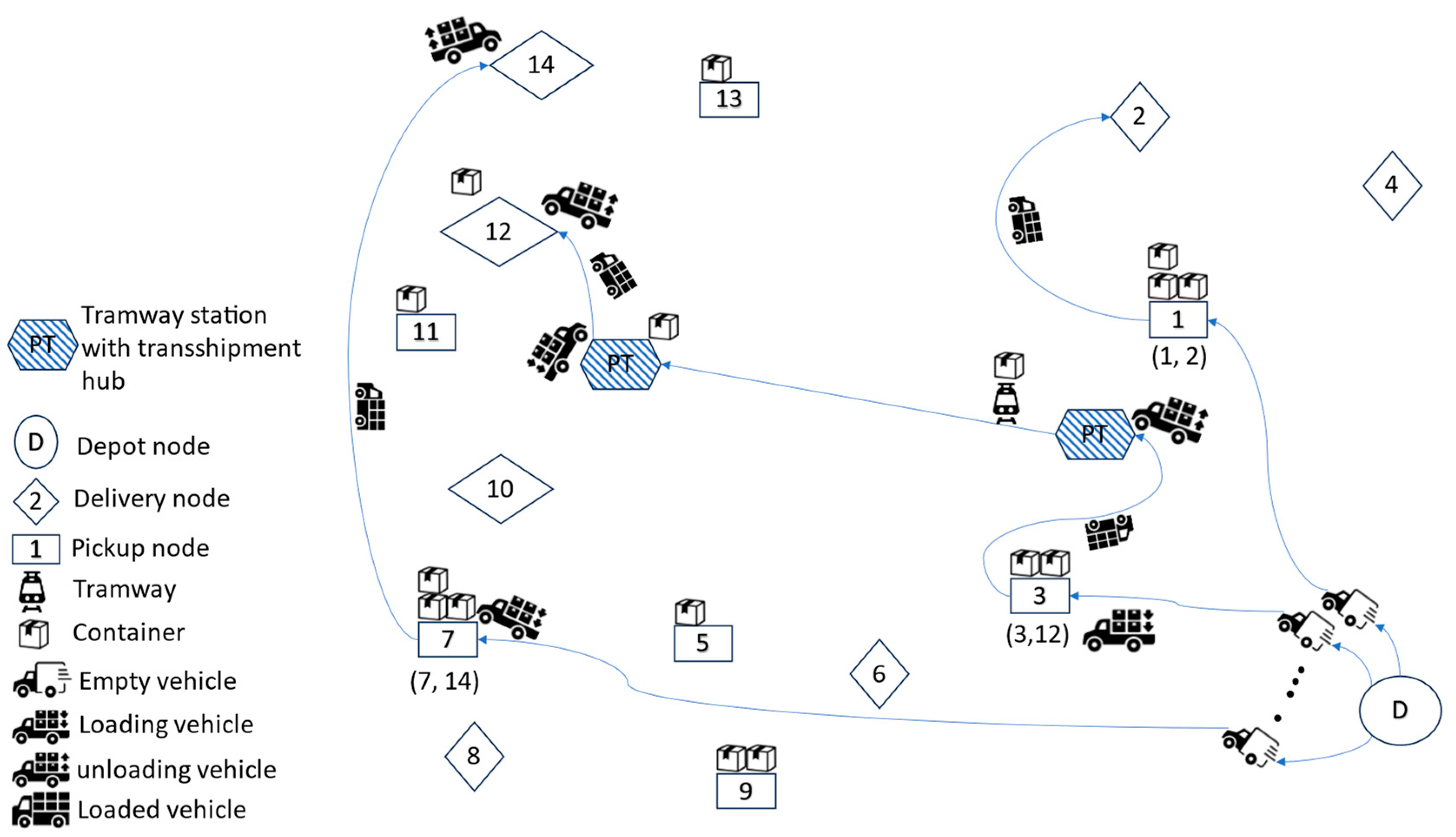
To illustrate the shipment flow within the proposed multimodal delivery system, Figure 1, presents a simplified operational scenario based on the custom-built environment. It shows how goods are picked up from designated pickup nodes, optionally transferred through tramway-based transshipment hubs, and ultimately delivered to their respective delivery nodes. The figure depicts the entire process, including the depot origin, trans-shipment handling, container movement, and vehicle states (empty, loading, unloading, and loaded), thereby clarifying the sequence of actions from sender to recipient in the integrated logistics network.

3.2. Data

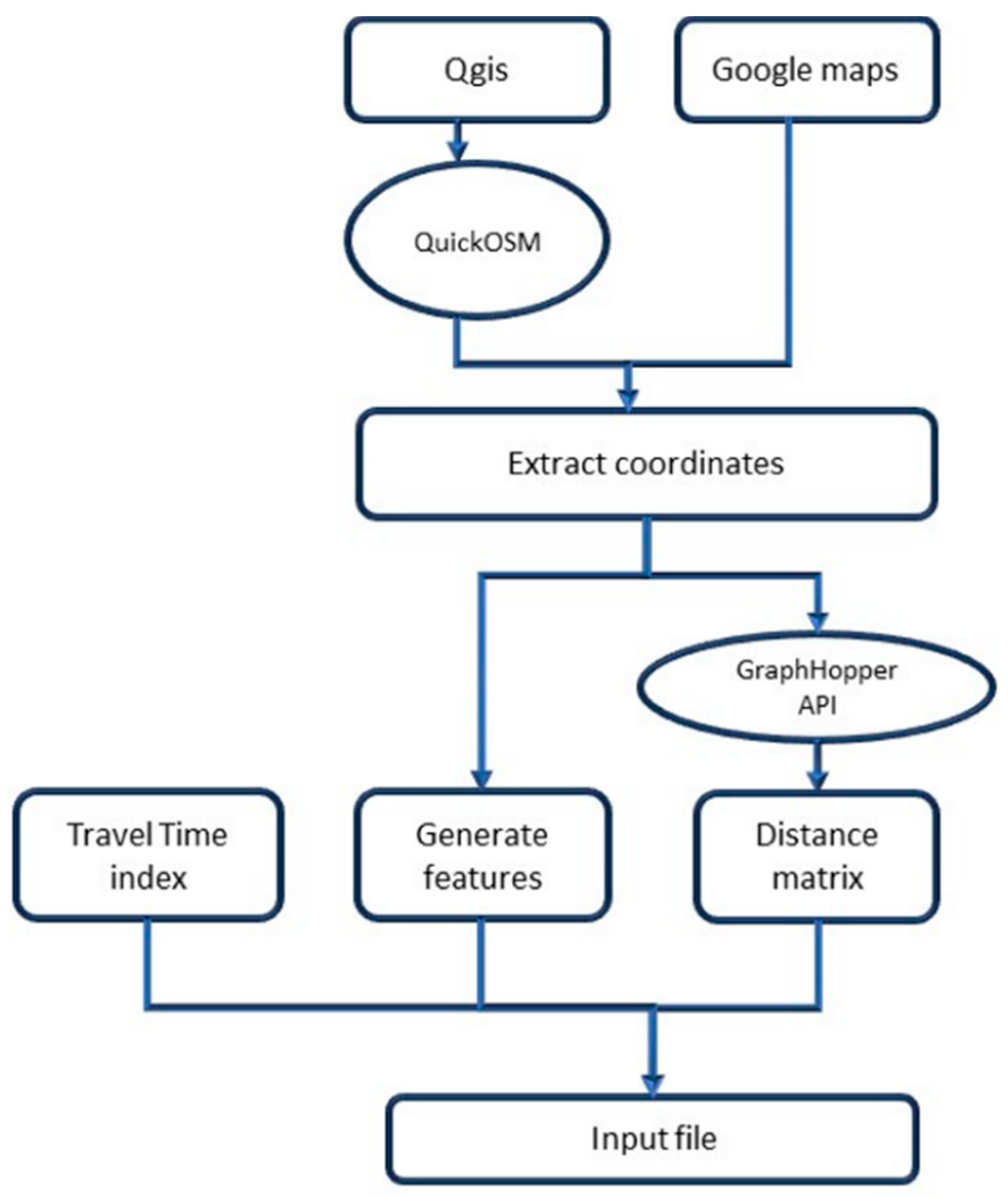
The data utilized in this case study were taken from OpenStreetMap and verified through Google Maps. The procedure utilized multiple custom algorithms to extract the coordinates of different commercial and logistical locations, including the port of Casablanca and the major shopping mall in the city. These coordinates were further enhanced by generating features such as time windows and the demand quantity. The demand data were generated randomly for each delivery node in the form of an intermodal container; in practice, this means that a delivery node requests one cargo container or up to three containers. The time windows were generated randomly as we could not collect real-life opening and closing time windows for these shops. The generated time windows spanned 7 am to 8 pm, and each node could have different time windows regarding when it could be open. Another feature that was generated was the service time; this feature was shared across all nodes, and it was generated randomly for all nodes.

The overall process of data extraction, feature generation, and input file preparation is illustrated in Figure 2. below.

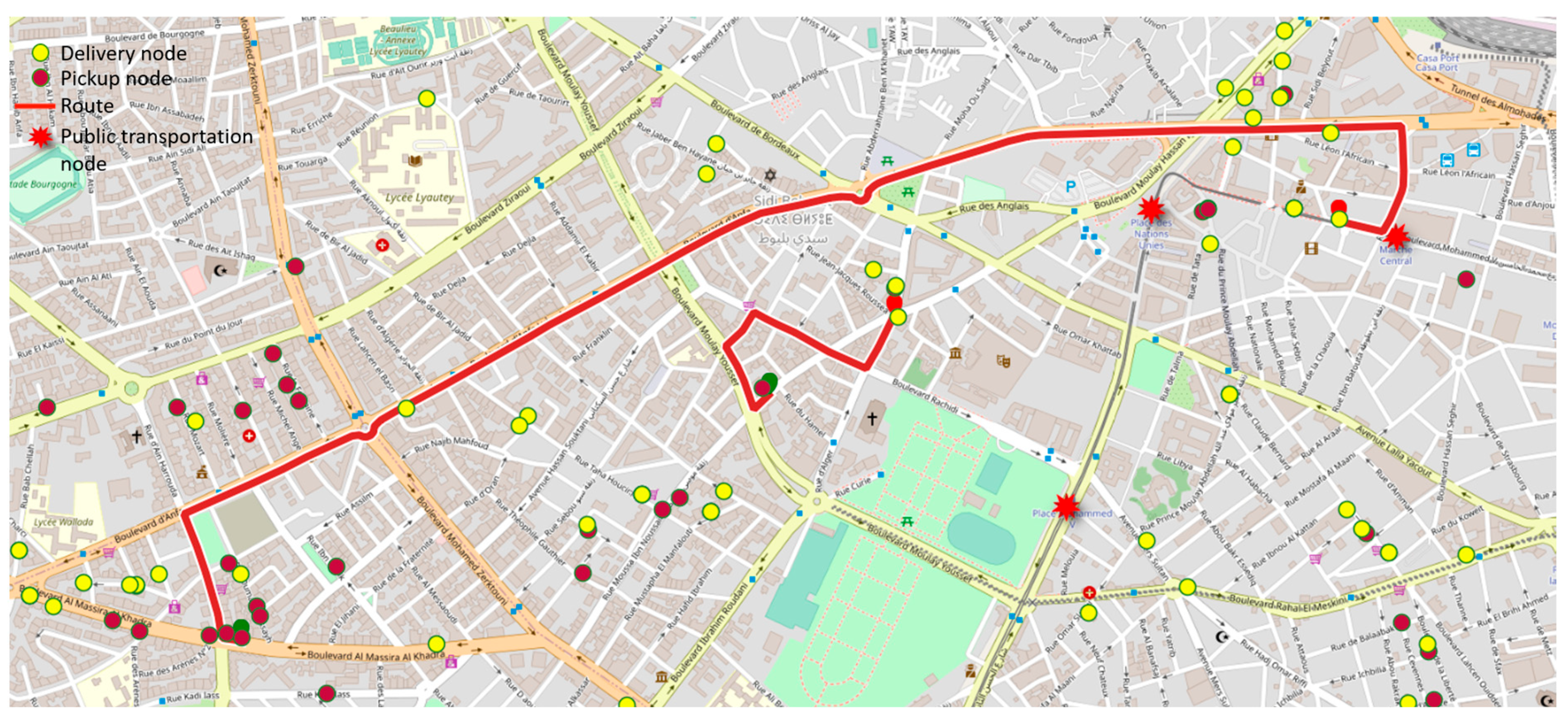
Once the input file was prepared, the generated delivery nodes, pickup nodes, public transportation nodes, depot nodes were visualized spatially to assess their distribution across the city. Figure 3 presents the projection of these nodes.

The depot nodes and public transportation nodes were not given any demand in the model, and it was assumed that the depot node was open to all vehicles for the entire 24 h of the day. The trips for public transportation were taken from real-life GTFS data for the tramways of Casablanca, and the time windows for public transportation were set to 20 min before the first trip from the given station to 20 min after the last trip from the last station. By generating random time windows for the pickup and delivery nodes, we could simulate real-world variability and unpredictability, making the model more robust.

The distance matrix was calculated through a custom script that utilized the GraphHopper API, using its services for route calculations. It was chosen as it provides the ability to calculate the distance between two coordinates without considering the effects of traffic, accidents, or other real-time disruptions. Once the distance matrix was generated, a custom Python 3.13.3 algorithm was used to verify that the matrix generated was nonnegative, square-shaped, and symmetrical. To better illustrate the network of nodes and the corresponding routes generated, Figure 4, presents the generated route between 4 different nodes, which was projected using the Qgis software version 3.38.3-Grenoble [22].

3.3. Logistics Environment and RL Framework

The use of a custom environment was essential for this research, as, to the best of our knowledge, no existing reinforcement learning (RL) environment specifically focuses on optimizing last-mile delivery operations by including the pickup and delivery operations while integrating public transportation networks into the delivery process. While reinforcement learning (RL) has been extensively applied in other disciplines, such as robotics and gaming, its application to urban logistics remains largely unexplored. This work aimed to fill this gap by developing a novel environment that models such problems and includes real-world complexities, such as bidirectional routing between nodes, time-dependent travel times captured through the travel time index (TTI), and time-sensitive tramway schedules. This environment enabled the testing and evaluation of a cutting-edge deep reinforcement learning (DRL) algorithm.

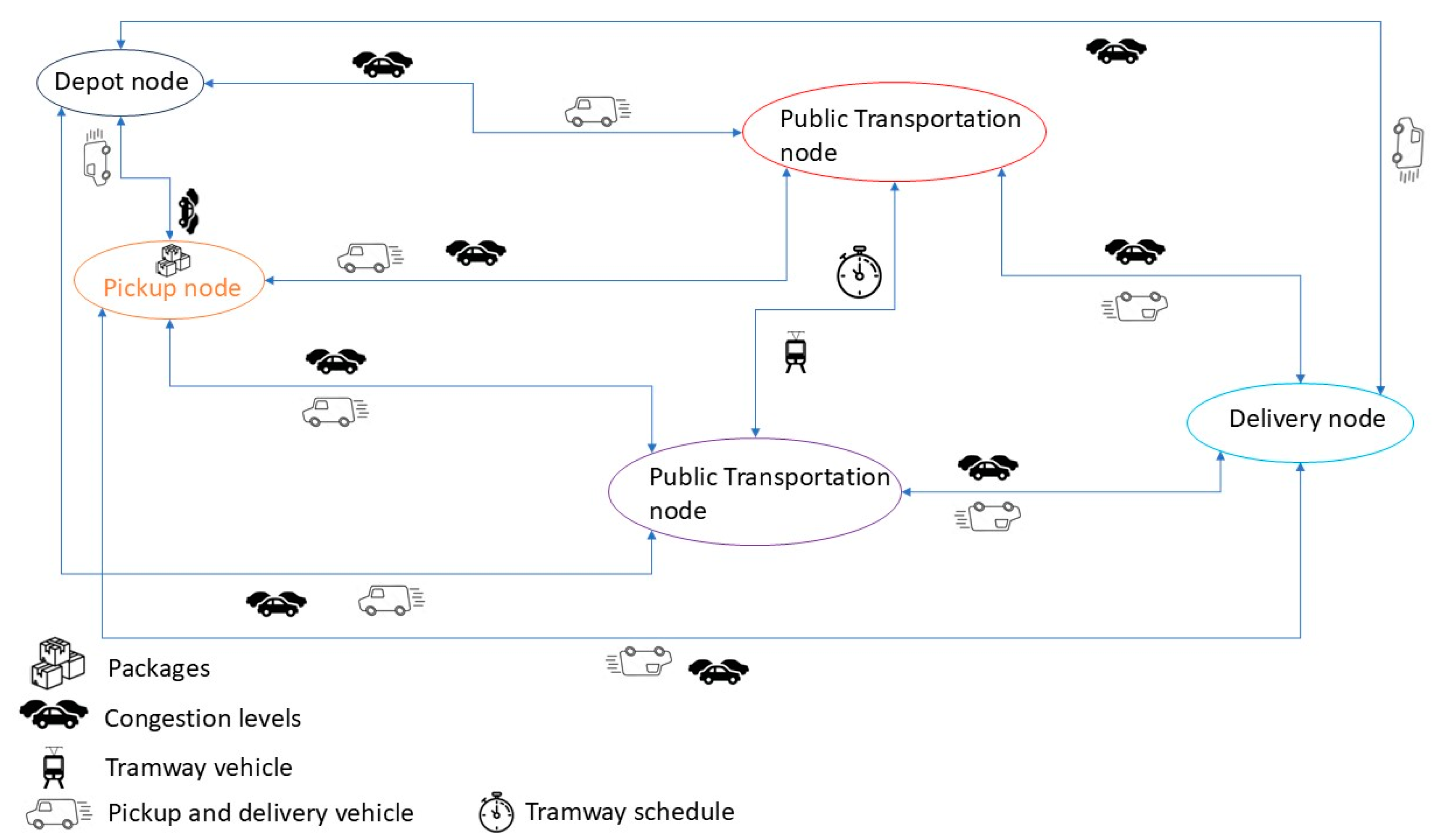
The environment is designed to model the complexities of last-mile delivery operations in Casablanca, where goods must be picked up and delivered across a network of nodes that present pickup and delivery locations, as well as public transportation stations and a single depot for pickup and delivery vehicles. Unlike existing environments that may focus on simpler or more abstract logistics tasks, this environment integrates important factors like the time windows (TW) associated with the nodes, the travel time index (TTI), and the tramway schedule for freight transportation trips using public transportation. Additionally, the freight network supports bidirectional routing (presented in the form of the arrows), allowing vehicles and goods to travel back and forth between the different nodes. This bidirectional structure reflects the dynamic nature of traffic and urban congestion. Figure 5, presents an example of the network and the different components. By embedding these factors, the environment mimics a few of the real-world challenges, ensuring that the RL agent learns to operate in a highly dynamic, time-sensitive environment.

• State space

The state space is a critical part in any attempt to use reinforcement learning. The initialization of the state provides the necessary information for the agent to operate effectively; in the framework of this study, it was designed to optimize the delivery and pickup of goods in the city of Casablanca. This custom environment is modeled as a graph, where the nodes represent the various interest points, such as pickup nodes, delivery nodes, public transportation nodes, and depot nodes. This combination, as well as the embedding of time windows (TW) and the travel time index (TTI) into the environment, increases the complexity and further reflects the dynamic nature of the pickup and delivery problem in the city.

The state space is structured as a dictionary instead of a tuple, which is the common way to structure a state in many existing reinforcement learning frameworks and libraries; given the complexity, and to allow more flexibility in the design of the state, the abovementioned structure was chosen.

$$S=\{\mathrm{“}\mathrm{previous}\_\mathrm{state}\mathrm{”}=None,\mathrm{“}\mathrm{current}\_\mathrm{state}\mathrm{”}=None\}$$

The previous_state is a deep copy of the current_state that is created at the end of each step or action taken by the agent and current_state as follows:

$$\begin{gathered} Current\_state=\{\mathrm{“}all\_nodes\_np\mathrm{”}:N,\mathrm{“}vehicle\_info\mathrm{”}:V,\mathrm{“}request\_queue\mathrm{”}:R,\mathrm{“}Publictransportation\mathrm{”}:PT, \\ \mathrm{“}visit\_counter\mathrm{”}:C,\mathrm{“}current\_time\mathrm{”}:t\} \end{gathered}$$

This structure provides a clear and comprehensive state representation, allowing the agent to have a detailed and dynamic understanding of the environment. While using a dictionary for state representation offers several advantages, there are also disadvantages to consider, such as the computational complexity and higher memory requirements compared to tuples. There is also reduced compatibility with many existing reinforcement learning frameworks and libraries that are designed to work with tuples for state representation.

• Action space

The action space defines the set of all possible actions that can be taken by the agent at any given time. In our work, the action space is discrete, meaning that the agent can choose from a finite set of actions numbered from 0 to 5. In each step, a single action can be executed, making the entire process of vehicle movement, pickup, and delivery a centralized process that is applied to all vehicles at the same time. Thus, when the agent decides to move a vehicle, all vehicles are moved, even if no pickup or delivery has been executed. This centralized approach ensures coordinated actions across the fleet and potentially optimizes the overall logistics operation.

The flowcharts representing the agent’s available actions are presented below.

The first action, presented in Figure 6, demonstrates the vehicle movement process, showcasing how the agent needs to wait to perform the request assignment action before starting the movement of the vehicle. Otherwise, it risks incurring large penalties, which can lower any rewards obtained from this action.

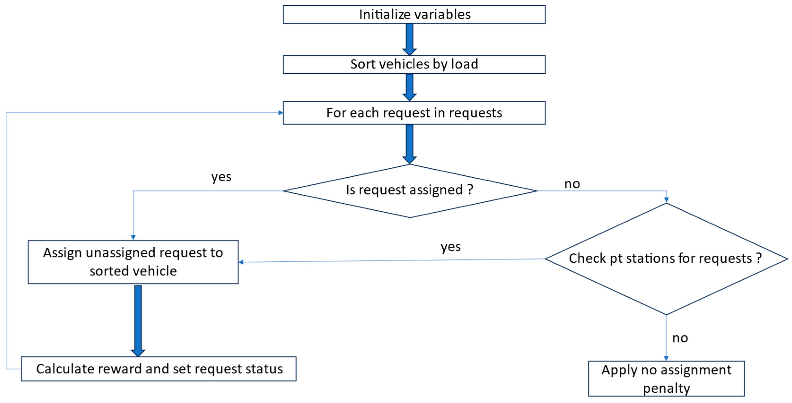
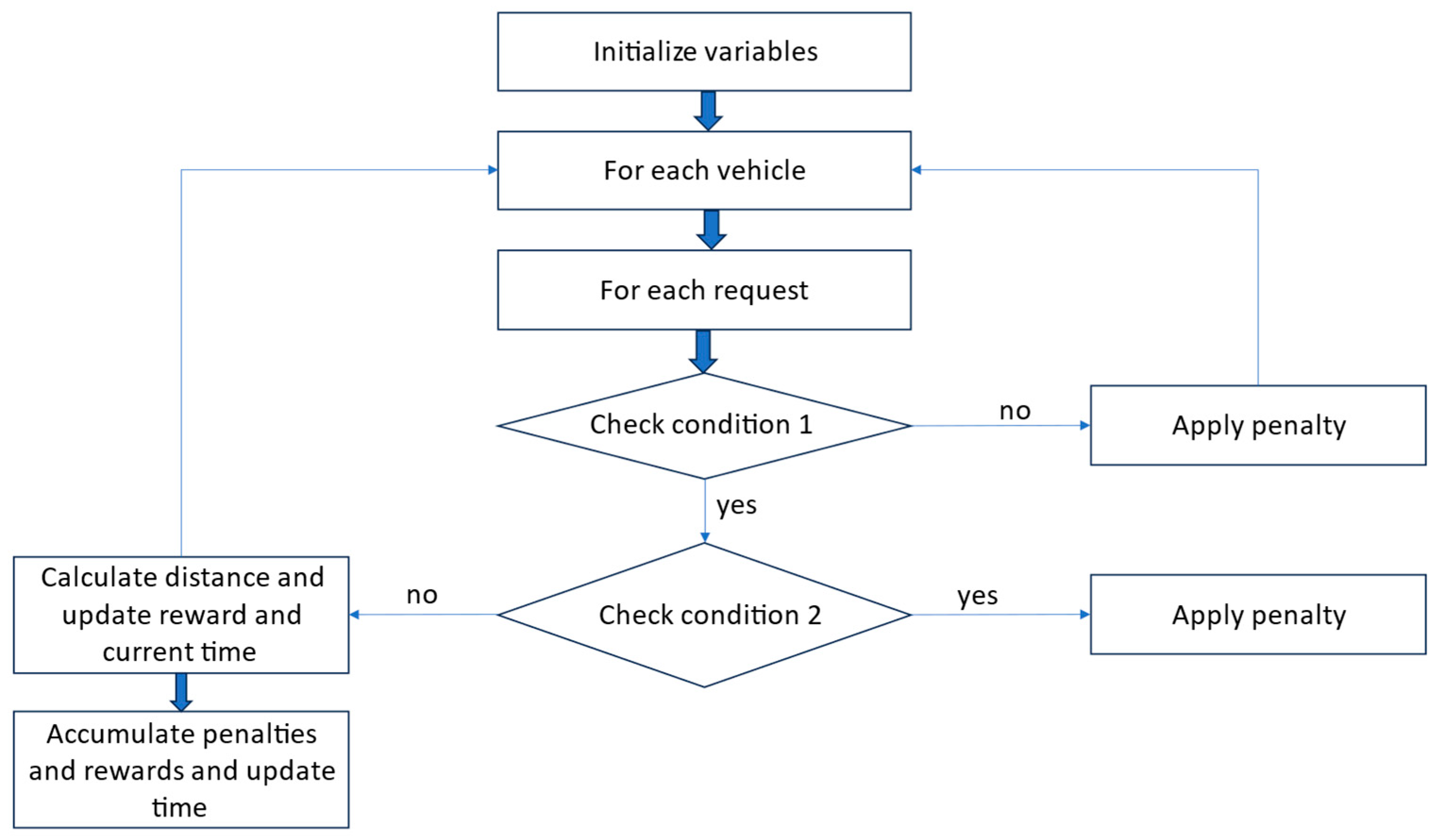
Figure 7 showcases the process of request assignment. It illustrates how the action systematically sorts vehicles by capacity to ensure efficient assignment. If a vehicle can accommodate the request’s size, the request’s status is changed, the vehicle package count is incremented, and a reward is granted to reflect successful allocation. In contrast, failing to assign a request triggers a penalty. The action prioritizes requests either waiting at a pickup node or arriving via a public transport vehicle.

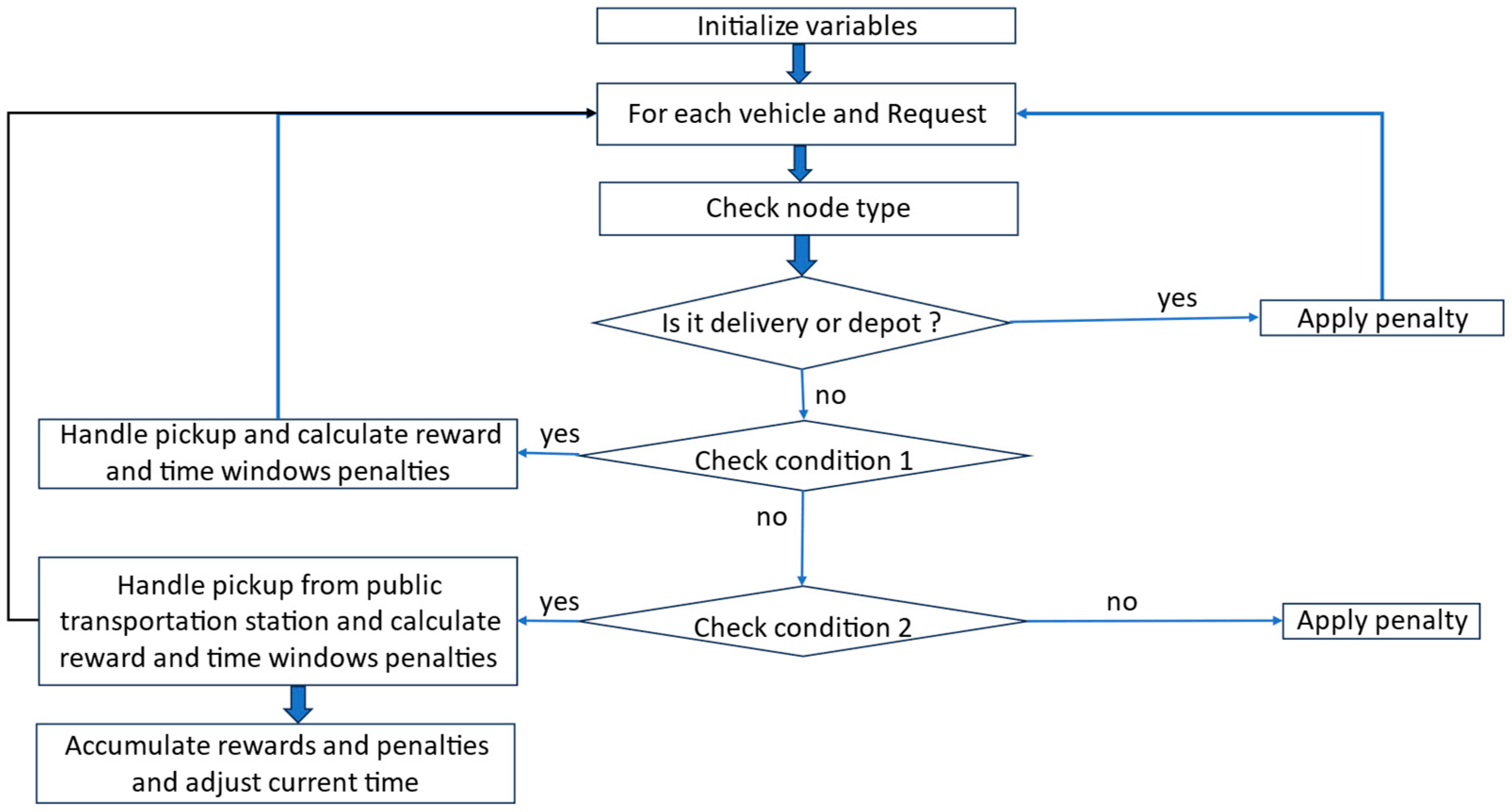
In Figure 8, the flowchart presents the pickup action, where each vehicle reads its current node and determines whether it matches the pickup location for the request assigned to them. If a pickup is valid, the system updates the request status and grants a reward and accounts for potential time window penalties. In contrast, if a vehicle attempts a pickup at a delivery node or depot without matching the request assigned to the vehicle, penalties are imposed.

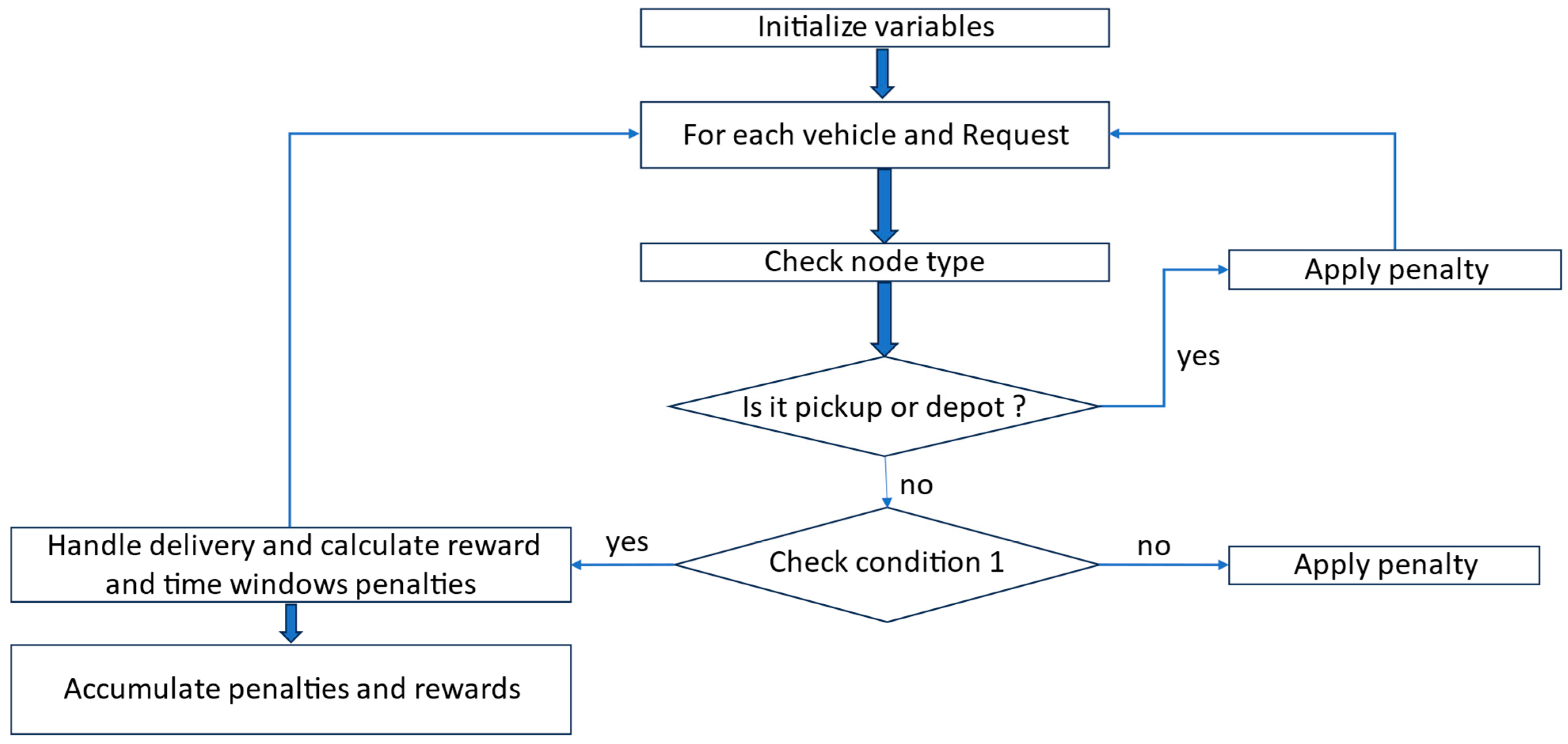
In Figure 9, the flowchart illustrates how, in the delivery action, the vehicles loop through pending requests to verify that they are at the correct delivery node. When a valid delivery occurs, the vehicle’s capacity is updated, and a substantial reward is granted. Again, if a vehicle is located at a pickup node or depot and tries to deliver, a penalty is imposed. This logic ensures that only legitimate deliveries are rewarded, while avoiding inefficient or incorrect actions.

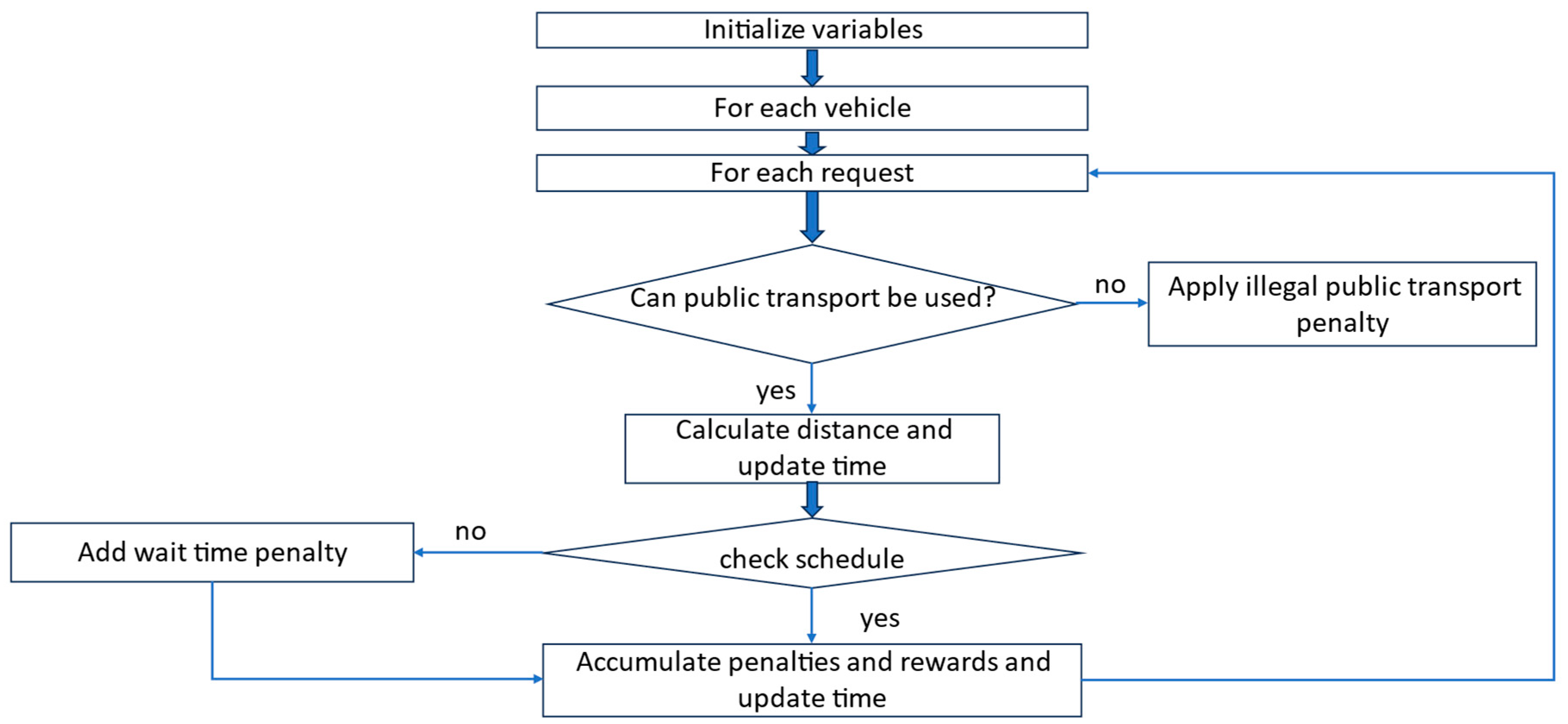
The flowchart in Figure 10 illustrates the logic within the public transportation action, where each request that is eligible for transport through public transportation is assessed against a corresponding trip’s origin and destination, the time window, and the departure schedule of the tramway. When a trip is found and the current time aligns with the available departure slot, the packages associated with the request are transported to the destination station associated with the trip and then picked up by another PD vehicle for final delivery. If a request cannot use public transport, the function applies a penalty, and, if the request needs to be kept at the trip origin station, a wait time penalty is applied.

The flowchart in Figure 11 encapsulates the logic of the return-to-depot function, which checks each vehicle’s status (no ongoing requests and no cargo) and, if it is idle, calculates the distance to its depot and updates the current time and reward. If a vehicle still carries packages, the function applies a penalty for attempting to return to the depot before delivering the assigned requests to the vehicle. By consolidating these outcomes, this action penalizes unnecessary movements while encouraging vehicles to return to the depot when unoccupied.

• Reward

The reward for the environment is a composite measure designed to evaluate the overall performance of the vehicle routing and request handling, as well as the efficient use of public transportation:

$$\begin{array}{l}reward=reward\_r\_depot+reward\_action\_mvt+illegal\_pt\_use\\ +reward\_action\_pt+assign\_request\_reward\\ +pickup\_reward+delivery\_reward\end{array}$$

• Algorithmic workflow

The following pseudocode Algorithm 1, summarizes the core logic of our learning and environment interaction cycle, including state transitions, action execution, and PPO-based policy training.

Algorithm 1. Algorithmic workflow of the deep reinforcement learning framework for multimodal last-mile delivery

Input: Environment config (vehicle data, nodes, requests, PT lines, distance matrix, TTI) Output: Trained PPO policy ${\pi }_{\mathsf{\theta }}$ for optimized delivery decisions 1: Initialize PPO policy ${\pi }_{\mathsf{\theta }}$$\mathrm{and}\mathrm{value}\mathrm{network}{V}_{\mathsf{\theta }}$ 2: Initialize simulation environment with config 3: for each episode do 4:  Reset environment state and time 5:  for t = 1 to T (until all requests handled or max steps reached) do 6:   Observe current state (vehicles, requests, nodes, PT, time) 7:   $\mathrm{Sample}\mathrm{action}{a}_{\mathrm{t}}$ ∈ {assign, pickup, deliver, move, use PT, return to depot} 8:   $\mathrm{Execute}{a}_{\mathrm{t}}$ in environment: 9:     ▸ If assign → allocate unassigned request to suitable vehicle 10:    ▸ If pickup → load container at pickup node or PT station 11:    ▸ If deliver → unload at delivery node if time window valid 12:    ▸ If move → relocate vehicle to target node (using TTI-adjusted time) 13:    ▸ If use PT → hand over container to tramway if schedule tolerates 14:    ▸ If return → send idle vehicle back to depot 15:   Compute step reward $r_{\mathrm{t}}$ (includes penalties and pickup and delivery bonuses) 16:   Accumulate transition in PPO rollout buffer $(s_{\mathrm{t}}$$,a_{\mathrm{t}}$$,r_{\mathrm{t}}$$,s_{\mathrm{t}+1}$) 17: end for 18: Update ${\pi }_{\mathsf{\theta }}$$\mathrm{and}{V}_{\mathsf{\theta }}$ using PPO with collected episode trajectories 19: end for

3.4. Proximal Policy Optimization

Proximal policy optimization, also known as PPO, is a widely used reinforcement learning algorithm designed to train agents to make decisions through trial and error. It belongs to the family of policy gradient methods, where the agent improves its behavior by adjusting a decision policy based on feedback from the environment.

PPO was first introduced in [23]. The aim was to develop a reinforcement learning algorithm that combines the benefits of trust region policy optimization (TRPO) with the simplicity and efficiency of standard gradient descent. Its main goal is to improve the policy while avoiding abrupt changes that could destabilize the training.

The core idea of PPO is to use a surrogate objective function to ensure that the new policy does not deviate too far from the old policy after an update. This helps to maintain stability and avoids destructive updates.

The surrogate objective for PPO can be written as follows (1):

$$L^{CLIP}\left(\mathsf{\theta }\right)=E_t\left[\min \left(r_t\left(\mathsf{\theta }\right)\widehat{A_t},\mathrm{clip}\left(r_t\left(\mathsf{\theta }\right),1-\mathsf{ϵ},1+\mathsf{ϵ}\right)\widehat{A_t}\right)\right],$$

(1)

where

• $r_t\left(\mathsf{\theta }\right)={\displaystyle \frac{{\mathsf{\pi }}_{\mathsf{\theta }}\left(a_t|s_t\right)}{{\mathsf{\pi }}_{{\mathsf{\theta }}_{\mathrm{old}}}\left(a_t|s_t\right)}}$ is the probability ratio of the new and old policies;
• $\widehat{A_t}$ is the advantage function at time step t;
• $\mathsf{ϵ}$ is the clipping range.

This clipping mechanism limits the update size, ensuring that the policy does not change too drastically. Another important equation is the entropy regularization equation, and it is defined as (2)

$$L_{\mathrm{entropy}}\left(\mathsf{\theta }\right)=L^{CLIP}\left(\mathsf{\theta }\right)+\mathsf{\beta }H\left[{\mathsf{\pi }}_{\mathsf{\theta }}\right],$$

(2)

• $\beta$ is a weight that controls the contribution of the entropy term;
• $H\left[{\pi }_{\theta }\right]$ is the entropy of the policy.

The weight $\beta$ is the critical part of the exploration strategy in Scenario 1 and Scenario 2. While it remains stable in Scenario 2 (standard PPO), in Scenario 1 (segmented training), a custom script in the training algorithm allows the reduction of $\beta$ by 10% whenever the mean reward falls below the target reward threshold. This dynamic adjustment encourages more exploitation as the training progresses and the model nears its optimal policy.

The epsilon-greedy exploration strategy, employed in Scenario 3 (PPO with epsilon-greedy), is designed differently because it is external to the PPO objective function. Epsilon-greedy is applied during action selection at each step of the training process, where the agent takes a random action with probability ϵ or selects the action that maximizes the expected reward with probability 1 − ϵ. This exploration mechanism decays over time, allowing more exploitation as the training advances.

These scenarios are designed to test both internal entropy regularization (via β in PPO) and external exploration mechanisms (via epsilon-greedy). Scenario 1 allows for flexible exploration control by adjusting β based on the reward performance; Scenario 2 maintains stable exploration with constant entropy; and Scenario 3 introduces an entirely different exploration–exploitation balance through the epsilon-greedy mechanism, offering insights into how each method impacts learning and performance.

Other important hyperparameters are as follows.

• Learning rate: controls the step size of policy updates in the Adam optimizer.
• Clip range: limits the extent of policy updates.
• Gamma: the discount factor, which determines how much the algorithm values future rewards.
• Batch size: refers to the number of samples used in each optimization step.
• N steps: the number of steps taken in the environment before an update occurs.
• N epochs: the number of times that the algorithm passes through the batch of data to perform gradient updates.
• Total timesteps: the duration of training.
• Exploration fraction: the proportion of the total timesteps where the exploration rate decays from epsilon start to epsilon end.

In

Table 1. Hyperparameters for each scenario (data source: authors’ collaboration).

Hyperparameter	Scenario 1: Segmented Training	Scenario 2: Standard PPO	Scenario 3: PPO with Epsilon-Greedy
Environment ID	CustomEnv-v9	CustomEnv-v9	CustomEnv-v9
Entropy Coefficient	0.5 (updated per chunk based on reward)	0.5	0.5
Learning Rate	linear_schedule (0.0005)	linear_schedule (0.0005)	linear_schedule (0.0005)
Clip Range	linear_schedule (0.2)	linear_schedule (0.2)	linear_schedule (0.2)
Gamma	0.923453699	0.923453699	0.923453699
Batch Size	64	64	64
N Steps	3072	3072	3072
N Epochs	10	10	10
Total Timesteps	5,000,000 (divided into chunks)	500,000	500,000
Chunks	10	Not applicable	Not applicable
Timesteps per Chunk	500,000	Not applicable	Not applicable
Target Reward Threshold	1,400,000	Not applicable	Not applicable
Best Chunk	Selected based on highest mean reward	Not applicable	Not applicable
Epsilon Start	Not applicable	Not applicable	1
Epsilon End	Not applicable	Not applicable	0.1
Exploration Fraction	Not applicable	Not applicable	0.1

, we present the values given to each hyperparameter and for each scenario.

4. Findings

In this section, six sets of experiments are presented. Three of these experiments include public transportation as a possible action for the agent and the rest do not. Below is a brief description of the experiments conducted.

• Experiment A: Standard PPO with linear scheduler for learning rate, clip range, and a fixed exploration rate, where the use of public transportation is allowed.
• Experiment B: Standard PPO with the same settings, but the exploration rate is managed by an ε-greedy strategy and the use of public transportation is not allowed.
• Experiment C: Standard PPO with the same settings as Experiment A, but the use of public transportation is not allowed for the agent.
• Experiment D: Segmented PPO with linear scheduler for learning rate, clip range, and a fixed exploration rate, where the use of public transportation is allowed.
• Experiment E: Segmented PPO with the same settings as Experiment D, but the use of public transportation is not allowed.
• Experiment F: Standard PPO with the same settings as Experiment B, but public transportation is allowed for the agent.

These experiments aimed to evaluate and understand the impact of integrating public transportation into the delivery network, as well as the impact of different exploration strategies on the performance of the PPO algorithm in solving the custom pickup and delivery problem with time windows, with and without the use of public transportation.

The results are presented in the following charts and tables, which illustrate the performance metrics, collected through TensorBoard and a custom logging algorithm. The metrics include the mean reward per episode, the smoothed cumulative reward per episode, and convergence behavior and loss metrics for each experiment.

4.1. Statistical Overview

In this section, we provide a detailed statistical analysis of the performance metrics obtained from the six sets of experiments. The focus is on comparing the mean episode reward and length, the median episode reward and length, the standard deviation (SD) of the episode reward and episode length, the minimum and maximum episode length and reward, the true completion rates, and the run times across all experiments. These metrics are important in evaluating the effectiveness of integrating public transportation and different exploration strategies into the PPO algorithm. Experiment A, which used standard PPO with a linear scheduler, serves as a baseline for comparison.

The statistical metrics discussed such as mean and median episode reward and length are presented in

Table 2. Statistical overview of the results of the experiments (data source: authors’ collaboration).

	Experiment A	Experiment B	Experiment C	Experiment D	Experiment E	Experiment F
Mean reward	1,430,009.93	−146,146.07	−145,602.96	1,494,693.74	−66,591.76	1,182,609.67
Median reward	1,374,990.58	−243,210.50	−247,164.09	1,460,770.33	−127,093.10	1,168,715.61
SD of episode reward	513,678.23	190,106.30	194,637.67	472,225.18	143,436.04	459,516.19
Minimum episode reward	490,311.65	−493,251.64	−452,334.76	31,071.58	−419,030.83	188,767.48
Maximum episode reward	3,098,554.17	115,837.03	123,523.46	2,990,046.78	161,765.49	2,608,778.97
Mean episode length	6200.54	6506.98	6370.22	7352.00	6381.09	7487.20
Median episode length	10,000.00	10,000.00	10,000.00	10,000.00	10,000.00	10,000.00
SD of episode length	4010.43	4722.01	4755.35	3806.89	4748.82	3834.87
Minimum episode length	1154.00	130.00	137.00	1006.00	105.00	972.00
Maximum episode length	10,000.00	10,000.00	10,000.00	10,000.00	10,000.00	10,000.00
True completion	46.15%	34.44%	35.86%	18.49%	23.83%	29.26%
Run time	3.36 h	3.48 h	3.60 h	3.64 h	2.50 h	3.20 h

.

Experiment D exhibits the highest mean reward (1,494,693.74), followed by Experiment A (1,430,009.93) and Experiment F (1,182,609.67), all of which include public transportation, suggesting that its availability positively impacts the agent’s ability to achieve higher rewards. Conversely, Experiments B, C, and E, which do not include public transportation, all have negative mean rewards, with Experiment E performing the best among them at −66,591.76, albeit still negative, indicating that the absence of public transportation significantly hinders the performance. The median rewards mirror this trend, with Experiment D having the highest median reward, indicating consistent performance, while Experiments B, C, and E show significantly negative median rewards, with Experiment C performing the worst. The standard deviation (SD) of the episode rewards is the highest in Experiments A (513,678.23) and D (472,225.18), indicating greater variability in rewards, likely due to the challenges of optimizing with public transportation. In contrast, Experiments B, C, and E exhibit lower variability, with Experiment E having the lowest SD (143,436.04), which might indicate more consistent but generally poor performance. The highest maximum episode rewards are observed in Experiment A (3,098,554.17), followed closely by Experiments D (2,990,046.78) and F (2,608,778.97), all involving public transportation. The minimum episode rewards are notably low in Experiments B and E, with Experiment B having the lowest at −493,251.64, reflecting the challenges faced without public transportation. The mean episode length is the longest in Experiments F (7487.20) and D (7352.0), suggesting that these agents were engaged in longer, potentially more complex tasks. The median episode length is consistently 10,000 across all experiments, indicating that many episodes likely ran for the maximum allowable length. The standard deviation of the episode length is the highest in Experiments C (4755.35) and B (4722.01), indicating greater variability in the episode duration, which might reflect inconsistent performance. Experiment A achieved the highest true completion rate at 46.15%, followed by Experiment C at 35.86% and Experiment B at 34.44%, showing that, while Experiment A performed well with public transportation, Experiment C still achieved a relatively high completion rate without it, suggesting that the fixed exploration strategy was somewhat effective. However, Experiment D has the lowest completion rate at 18.49%, indicating that, while it achieved high rewards, it struggled with overall task completion, potentially due to its segmented nature. Finally, Experiments D and C had the longest run times at 3.64 and 3.6 h, respectively, reflecting the more complex or challenging nature of these scenarios, whereas Experiment E had the shortest run time at 2.5 h, possibly due to the segmentation approach, leading to quicker but less effective learning.

4.2. Reward Analysis

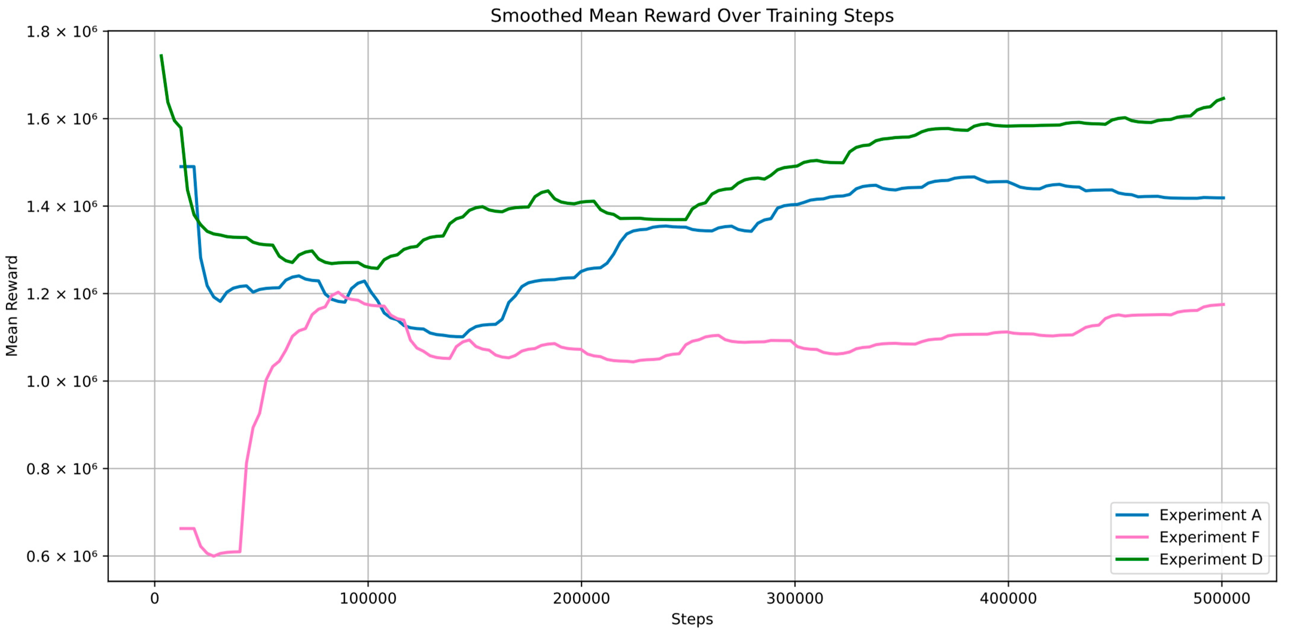
The smoothed mean rewards curves presented in the Figure 12, illustrate the performance of three distinct deep reinforcement learning experiments, corresponding to Experiments A, D, and F. Experiment A, represented by the light blue curve, starts with a high initial reward that dips significantly before gradually recovering and stabilizing at a moderate level. This behavior suggests that the agent initially struggles but eventually adapts and improves its performance over time. Experiment F, depicted by the pink curve, shows the lowest starting rewards early on, with a slower and less robust recovery, as can be seen from the explosive early increase and then the drop in rewards until it recovers. The final reward level remains lower than that of the other experiments, indicating that this approach might lead to less effective learning or instability in the agent’s ability to generalize its policy. Conversely, Experiment D, represented by the green curve, exhibits the most stable and consistent increase in rewards. Starting from a high point, the reward drops but then steadily rises and surpasses those of the other experiments, stabilizing at the highest level. This suggests that the combination of ε-greedy exploration with public transportation as an action allows the agent to explore more effectively and adapt its policy to achieve superior long-term performance. The graph is presented in Figure 12.

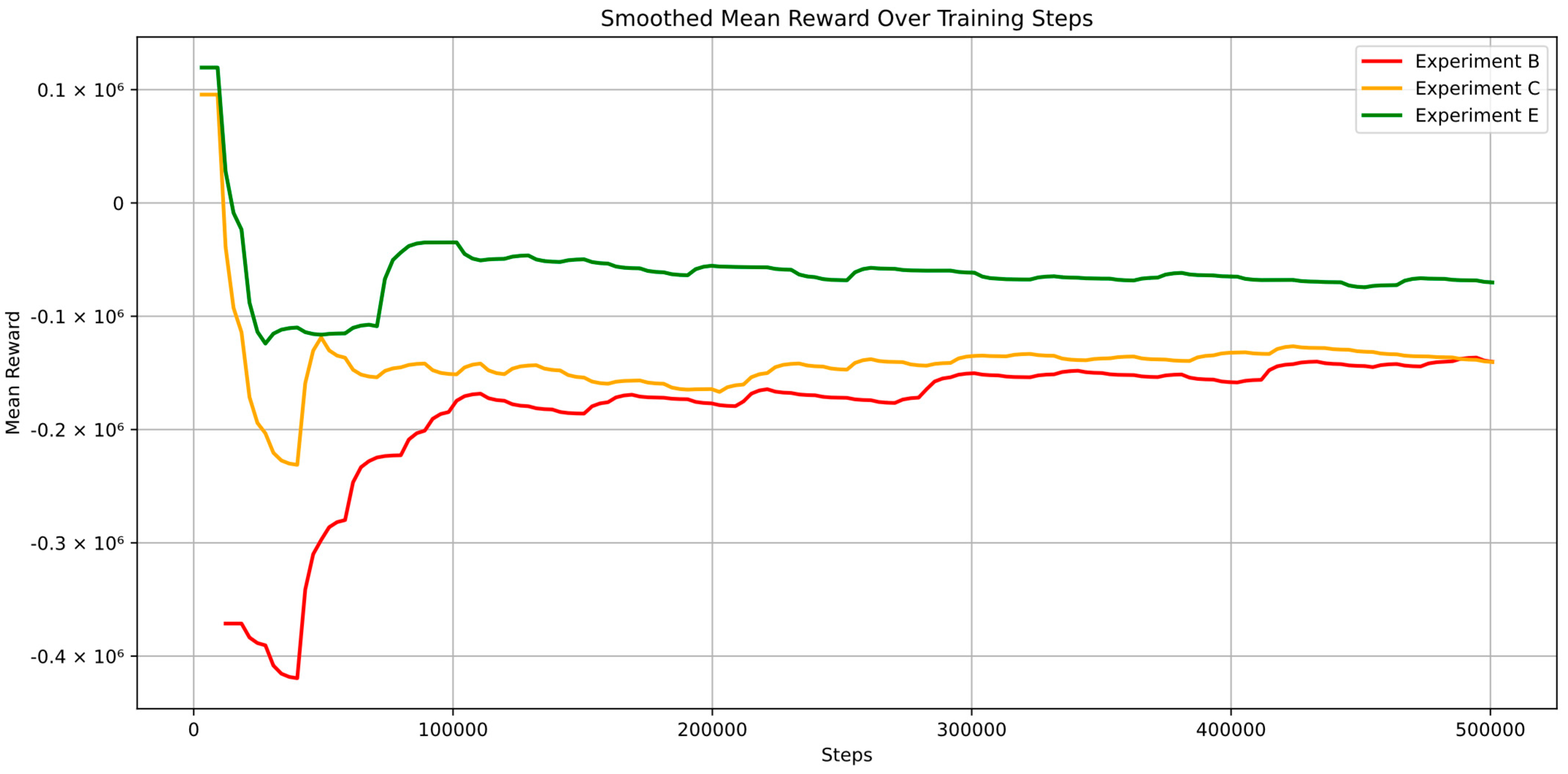
The graphs in Figure 13, presents the mean episode rewards over time for Experiments B, C, and E, each utilizing different configurations of the PPO algorithm, without including public transportation as an action.

In Experiment B, represented by the red curve, standard PPO with an ε-greedy exploration strategy was employed, excluding public transportation. The reward curve starts from a negative value and gradually improves as the experiment progresses. This trend indicates that, while the ε-greedy strategy initially leads to less effective actions, the agent eventually learns and improves its policy, although it struggles to achieve positive rewards.

Experiment C, depicted by the orange curve, uses standard PPO with a fixed exploration rate and no public transportation. The curve begins at a slightly higher point compared to Experiment B but experiences a significant drop, followed by gradual stabilization close to zero. This behavior suggests that the agent quickly settles into a policy that it struggles to improve upon. The relatively stable yet negative rewards imply that the fixed exploration rate might not provide sufficient diversity in actions, leading to suboptimal policy performance in the absence of public transportation.

The green curve represents Experiment E, which is based on a segmented PPO approach with a fixed exploration rate and no public transportation. This curve starts similarly to the green curve but experiences a more pronounced initial drop before stabilizing at a lower value than in Experiment C. This indicates that the segmented approach, while intended to enhance learning by breaking down the training into chunks, does not lead to better outcomes in this case. The rewards stabilize below zero, suggesting that the agent struggles even more to develop an effective policy without the diversity and exploration provided by public transportation.

4.3. Training Metrics

In scientific research articles focused on the performance of reinforcement learning algorithms, it is common to present plots for various metrics to visualize and analyze the results. However, in this study, there were six distinct scenarios and nine metrics to monitor, which would have resulted in an excessive number of plots. To maintain clarity and conciseness, we summarize the training metrics in a comprehensive

Table 3. Performance statistics of PPO training across Scenarios A–F (data source: authors’ collaboration).

Scenario	Metric	Best	Worst	Average	Median	Std Dev
A	Approx kl	0.021064	0.4936398	0.005452	0.004596	0.00471
	Clip fraction	0.702018	0.020573	0.306074	0.301709	0.126823
	Clip range	0.198771	0.000934	0.099853	0.099853	0.057642
	Entropy loss	1,703,476.0000000	1,790,066.0000000	1,766,089.0000000	1,768,588.0000000	0.015771
	Explained variance	0.924288	3,212,313.0000000	0.185494	0.238767	0.638572
	Learning rate	0.000497	0.000002	0.00025	0.00025	0.000144
	Loss	−0.84748	−0.967014	−0.89558	−0.894565	0.02112
	Policy gradient loss	0.004637	−0.062024	−0.012961	−0.005867	0.016352
	Value loss	0.06895	0.000003	0.002961	0.000669	0.006714
B	Approx kl	0.082758	0.8430216	0.008989	0.005244	0.012389
	Clip fraction	0.927897	0.01263	0.35048	0.306169	0.203677
	Clip range	0.198771	0.000934	0.099853	0.099853	0.057642
	Entropy loss	1,381,023.0000000	1,605,034.0000000	1,522,351.0000000	1,532,232.0000000	0.045326
	Explained variance	0.972555	1,730,443.0000000	0.136243	0.001664	0.452961
	Learning rate	0.000497	0.000002	0.00025	0.00025	0.000144
	Loss	−0.531908	−0.866015	−0.775785	−0.77645	0.03515
	Policy gradient loss	0.036296	−0.081211	−0.017126	−0.013936	0.024131
	Value loss	0.101492	0.000139	0.004276	0.000433	0.010965
C	Approx kl	0.057913	0.000002	0.007753	0.005747	0.008761
	Clip fraction	0.866178	0.014388	0.339163	0.295492	0.1697
	Clip range	0.198771	0.000934	0.099853	0.099853	0.057642
	Entropy loss	1,378,674.0000000	−160,563.0000000	1,527,851.0000000	1,535,511.0000000	0.045001
	Explained variance	0.921293	1,393,859.0000000	0.108631	−0.002808	0.435055
	Learning rate	0.000497	0.000002	0.00025	0.00025	0.000144
	Loss	−0.696797	−0.880749	−0.783104	−0.781007	0.034392
	Policy gradient loss	0.03263	−0.07198	−0.020108	−0.014294	0.024309
	Value loss	0.093117	0.000108	0.003002	0.000308	0.008273
D	Approx kl	0.055613	0.7750738	0.007347	0.00535	0.007715
	Clip fraction	0.648828	0.08112	0.342833	0.341846	0.108793
	Clip range	0.198771	0.000934	0.099853	0.099853	0.057642
	Entropy loss	1,514,976.0000000	1,770,025.0000000	1,706,271.0000000	1,711,455.0000000	0.041378
	Explained variance	0.927973	6,751,225.0000000	0.223558	0.156751	0.772326
	Learning rate	0.000497	0.000002	0.00025	0.00025	0.000144
	Loss	−0.320424	−0.461514	−0.386518	−0.383137	0.023515
	Policy gradient loss	0.001461	−0.068318	−0.017122	−0.00766	0.018469
	Value loss	0.012937	0.000002	0.001995	0.000232	0.002756
E	Approx kl	0.072838	0.5658755	0.010673	0.005262	0.014033
	Clip fraction	0.875651	0.102116	0.335788	0.311735	0.139029
	Clip range	0.198771	0.000934	0.099853	0.099853	0.057642
	Entropy loss	1,037,567.0000000	−150,552.0000000	1,333,937.0000000	1,336,079.0000000	0.094787
	Explained variance	0.960174	3,215,885.0000000	0.211177	−0.001516	0.489234
	Learning rate	0.000497	0.000002	0.00025	0.00025	0.000144
	Loss	−0.203683	−0.36805	−0.277282	−0.274477	0.029887
	Policy gradient loss	0.022793	−0.069261	−0.017868	−0.014305	0.020922
	Value loss	0.0136	0.00005	0.001261	0.00013	0.002216
F	Approx kl	0.023518	0.5252077	0.005543	0.004211	0.004815
	Clip fraction	0.628027	0.014876	0.311628	0.307568	0.117836
	Clip range	0.198771	0.000934	0.099853	0.099853	0.057642
	Entropy loss	1,708,181.0000000	1,788,501.0000000	1,761,512.0000000	1,766,203.0000000	0.017273
	Explained variance	0.925045	2,532,989.0000000	0.209581	0.064022	0.491739
	Learning rate	0.000497	0.000002	0.00025	0.00025	0.000144
	Loss	−0.848403	−0.953544	−0.894313	−0.893315	0.018563
	Policy gradient loss	0.007671	−0.068237	−0.014439	−0.005873	0.017312
	Value loss	0.06292	0.000004	0.002749	0.000398	0.005766

, allowing for the more streamlined presentation of the results.

The results from the six experiments present a nuanced picture of how different training strategies impact various performance metrics in reinforcement learning, specifically when using the PPO algorithm under different conditions. These experiments aimed to evaluate the effectiveness of different exploration strategies and the role of public transportation as an additional action for the agent. The metrics analyzed include approx_kl, clip_fraction, clip_range, entropy_loss, explained_variance, learning_rate, loss, policy_gradient_loss, and value_loss.

In Experiment A, where standard PPO with a linear scheduler for the learning rate and clip range was used and public transportation was allowed, there was a relatively stable training process. The approx_kl metric, which measures the divergence between the new and old policies, had a low average value, suggesting that policy updates were moderate and controlled and did not deviate significantly from previous policies. However, since approx_kl was extremely low even in the worst case, this indicates that the policy updates were overly conservative, potentially limiting exploration. The clip_fraction value was moderate, implying that policy clipping occurred with some frequency but not excessively, which is desirable as it indicates that the policy did not require substantial corrections during training. The entropy_loss metric, which reflects the randomness in the policy, was consistently negative with a low standard deviation, indicating that the exploration process was stable and the policy did not overly rely on randomness, meaning that the policy became more deterministic over time. However, the consistently low entropy might suggest premature convergence if exploration was insufficient in early training. Overall, Experiment A suggests that incorporating public transportation helps to provide additional action diversity, potentially reducing the need for drastic policy corrections.

Experiment B, on the other hand, used standard PPO with an ε-greedy exploration strategy and did not allow public transportation. This setup resulted in higher variability across several metrics, particularly clip_fraction and policy_gradient_loss, suggesting less stability in the policy updates. The approx_kl metric was also higher on average compared to Experiment A, indicating that the policy updates were more aggressive. This could indicate more flexible policy adaptation, potentially leading to less controlled learning. The variability in explained_variance further underscores the instability in this scenario, as the value function struggled to accurately predict future rewards consistently. While ε-greedy likely contributed to greater exploration, the absence of public transportation may have reduced the agent’s ability to experience diverse transitions, leading to more inconsistent learning. It remains to be confirmed whether the inclusion of public transportation directly enhances policy stability or interacts with other training variables.

Experiment C, which was similar to Experiment A but without public transportation, showed a slight increase in the average approx_kl and in clip_fraction and policy_gradient_loss. The absence of public transportation appears to have limited the agent’s exploration capacity, leading to a less diverse set of experiences and, consequently, a less stable learning process. The entropy_loss metric remained stable, but the overall performance in terms of explained_variance was less consistent. However, this variability could indicate that the agent was encountering more diverse states and struggling to generalize. This further suggests that the absence of public transportation influenced the exploration dynamics and the agent’s ability to generalize across different states effectively.

In Experiment D, the use of segmented PPO with a fixed exploration rate and the inclusion of public transportation produced mixed results. While the approx_kl and clip_fraction metrics were relatively stable, indicating a controlled policy update process, the explained_variance metric showed significant variability. This suggests that, while the segmented approach might help in stabilizing certain aspects of the training process, it also hinders the value function’s ability to consistently predict rewards. The variability in explained_variance might be attributed to the segmented nature of the training, where different segments exposed the agent to varying degrees of predictability. In other words, while segmenting helped to stabilize certain aspects of training, it may have made reward prediction more challenging in some state distributions.

Experiment E, which also used segmented PPO but without public transportation, had the lowest average loss and value_loss, indicating that the model was able to minimize errors effectively. However, this came at the cost of increased variability in several other metrics, particularly explained_variance. The results suggest that, while the segmented approach can be effective in minimizing immediate prediction errors, the absence of public transportation limits the agent’s ability to generalize across different states, leading to more inconsistency in the value function accuracy.

Finally, Experiment F, which combined the ε-greedy strategy with the allowance of public transportation, showed a return to more stable training dynamics. The approx_kl and clip_fraction metrics were more consistent with those observed in Experiment A, suggesting that the inclusion of public transportation and the adaptive ε-greedy exploration strategy helped to mitigate the instability. The overall stability in metrics such as policy_gradient_loss and value_loss indicates that the combination of an adaptive exploration strategy with the availability of diverse actions like public transportation can lead to a more balanced and effective learning process.

5. Discussion

5.1. Performance of Experiments with and Without Public Transportation

The comparison between experiments that included public transportation (Experiments A, D, and F) and those that did not (Experiments B, C, and E) reveals a significant impact on the agent’s performance in reinforcement learning tasks. Experiments A, D, and F consistently showed higher mean rewards, with Experiment D achieving the highest mean reward (1,494,693.74), followed by Experiment A (1,430,009.93). The inclusion of public transportation as an additional action seems to have facilitated broader exploration, providing the agent with a richer set of exploration opportunities, allowing it to achieve better policy optimization. This is further supported by indicators such as approx_kl and clip_fraction observed in these experiments, e.g., the relatively low and consistent approx_kl values, which indicate controlled policy updates. On the other hand, experiments without public transportation (B, C, and E) yielded negative mean rewards, with Experiment E performing slightly better than the others but still failing to achieve positive rewards. The absence of public transportation appears to have constrained the agent’s exploration capabilities, leading to less diverse experiences and, consequently, less effective learning. The higher variability in metrics such as clip_fraction and policy_gradient_loss in these experiments further underscores the instability in the training process when the agent’s action space is limited. However, it is worth noting that, while the reward-based performance was higher, the true completion rates varied. Experiment A had a 46.15% completion rate, while, in D, despite its high rewards, the process was completed only 18.49% of the time. This may indicate that the agent learned to exploit intermediate rewards rather than task fulfillment.

Furthermore, the reward curves from the graphs in Figure 11, depicting Experiments A, D, and F, further illustrate the differences in the learning dynamics associated with public transportation, including its contribution to more stable and consistent learning outcomes. Experiment D, for example, showed a steady increase in rewards, surpassing the other experiments and stabilizing at the highest level. In contrast, Experiment F exhibited a slower recovery in rewards, indicating that, while the ε-greedy exploration strategy might have delayed early performance due to increased exploration, the availability of public transportation helped to mitigate its negative effects. Experiment A, with its relatively moderate yet stable reward curve, demonstrates that a fixed exploration strategy with public transportation leads to a balanced learning process, allowing the agent to adapt effectively over time.

5.2. Evaluation of Exploration Strategies

The evaluation of different exploration strategies across the experiments provides insights into how these strategies interact with the agent’s ability to learn and generalize policies. For the ε-greedy exploration strategy, Experiments B and F demonstrate that its effectiveness is strongly influenced by the availability of public transportation. In Experiment F, where public transportation was allowed, combined with the ε-greedy exploration strategy, the agent was able to recover from the early variability and achieve high rewards. The metrics, such as the consistent approx_kl and clip_fraction values, indicate that the exploration was effective in discovering optimal policies. However, in Experiment B, where public transportation was not included, the ε-greedy strategy struggled significantly. The reward curve started from a negative value and only gradually improved, reflecting the challenges of achieving effective exploration in a limited action space. The higher variability in policy_gradient_loss and explained_variance further suggests that the ε-greedy strategy introduced instability, leading to less controlled policy updates and poorer overall performance.

In contrast, the fixed exploration strategy used in Experiments A and C demonstrated more consistent but less dynamic learning outcomes. In Experiment A, the fixed exploration rate, combined with public transportation, resulted in stable training dynamics and a moderate yet steady improvement in rewards. The controlled policy updates, as indicated by the metrics, suggest that this strategy is effective when the agent has access to a diverse set of actions. However, in Experiment C, where public transportation was absent, the fixed exploration strategy led to suboptimal performance, with the agent quickly settling into a less effective policy. The reward curve in Experiment C shows a significant drop followed by stabilization near zero, indicating that the fixed exploration strategy may only be effective when the agent has access to a sufficiently rich action space.

The segmented PPO approach, evaluated in Experiments D and E, also presents interesting findings. While segmentation was intended to enhance learning by breaking down the training into chunks, its effectiveness appeared to be contingent on the availability of public transportation. In Experiment D, the segmented approach, coupled with public transportation, resulted in the highest mean rewards and a steady increase in performance over time. However, this was accompanied by a low completion rate (18.49%), indicating that, while the agent learned to optimize the cumulative reward, it may have exploited intermediate objectives rather than consistently achieving full task completion. Additionally, the high variability in explained_variance suggests that the segmented nature of the training introduced challenges in accurately predicting rewards across different segments. In Experiment E, where public transportation was not available, the segmented PPO approach failed to achieve positive rewards, with the reward curve stabilizing well below zero. This outcome indicates that segmentation alone is insufficient to improve the learning outcomes and may even hinder the learning process if the action space is limited.

5.3. Insights and Future Research Perspectives

The findings from these experiments underscore the critical role of action diversity, such as the inclusion of public transportation, in enhancing the performance of deep reinforcement learning agents. Public transportation may enhance the exploration opportunities through providing a richer action space and contribute to learning stability, particularly when combined with effective exploration strategies like ε-greedy. Conversely, the absence of such diversity significantly hinders the performance, leading to negative rewards and greater instability in the training process.

Future research could explore the integration of more sophisticated exploration strategies that adapt dynamically based on the agent’s performance and the diversity of available actions. More research into the segmented PPO approach could clarify under which conditions segmentation improves policy learning, balancing stability and the learning speed without introducing instability, especially in areas where there are few action spaces. The authors of [24] proposed two novel modules called the Intrinsic Exploration Module with PPO (IEM-PPO) and Intrinsic Curiosity Module with PPO (ICM-PPO), which enhance the exploration efficiency through uncertainty estimation, and ICM-PPO relies on prediction errors to guide exploration. The authors performed their experiments in a MuJoCo environment. It would be valuable to evaluate the effects of these exploration strategies on the pickup and delivery operations in this new custom environment.

Moreover, exploring alternative forms of action diversity, beyond public transportation, could reveal new avenues by which to enhance agent performance. An example is the use of drones or robots instead of pickup and delivery vehicles, which could result in new challenges. For instance, introducing variable environmental conditions or adaptive task complexity might further enrich the agent’s learning experience, leading to more generalized and robust policies.

The idea of developing adaptable transshipment mechanisms is also promising. In the current setup, public transportation hubs act as static transfer points. Making these trans-shipment behaviors dynamic—based on demand, load, or scheduling constraints—could lead to more flexible and resilient logistics strategies. A related study [25] demonstrated how deep reinforcement learning agents can manage cargo placement and obstacle avoidance in roll-on/roll-off ships; a similar approach could be adapted to multi-modal freight networks.

Furthermore, anomaly detection is a promising direction for the integration of freight delivery with public transportation as it can allow the agent to detect anomalies in the delivery process and the location of packages without having to assign requests frequently. An interesting paper [26] proposed a deep learning-based framework that detects anomalies in connected and autonomous vehicles in real time. This concept could be adapted to monitor packages, detecting anomalies in the logistics process instead of focusing solely on vehicles.

Finally, it would be beneficial to conduct longitudinal studies that assess the long-term impacts of action diversity on the agent’s ability to generalize across different tasks and environments. These studies could provide deeper insights into how the richness of the action space influences the sustainability of the learning outcomes, offering guidance for the design of reinforcement learning systems that are both efficient and resilient.

6. Conclusions

This study has demonstrated the significant impact of integrating public transportation into training of deep reinforcement learning on pickup and delivery operations to optimize the performance of last-mile delivery operations in the city of Casablanca. By incorporating public transportation into the agent’s action space, we observed a significant improvement in the learning efficiency, policy stability, and overall performance. The experiments clearly showed that, when public transportation was included, the agent achieved higher mean rewards, more stable learning dynamics, and a richer set of exploration opportunities, leading to better policy optimization. In contrast, the absence of public transportation constrained the agent’s performance, resulting in negative rewards, greater variability, and less effective learning processes.

Experiment D surpassed all other experiments, with a mean reward of 1,494,693.74. Despite a reduced completion percentage of 18.49%, its use of public transportation and segmented training, which influenced the exploration coefficient, resulted in high mean rewards and a stable policy. However, this can also lead to challenges in accurately predicting rewards. Experiment A followed closely, with a mean reward of 1,430,009.93 and the best completion rate of 46.15%, proving that combining public transportation vehicles with a predetermined exploration plan can result in both substantial mean rewards and consistent task completion. Another finding that points to Experiment D as the best-performing scenario is the lowest value loss, recorded at 0.012937. This positions this scenario as the best in minimizing prediction errors. While some experiments, such as Experiment F, exhibited better stability in approx_kl and clip_faction, Experiment D remained superior overall.

Furthermore, this study highlighted the importance of the exploration strategy used. While the ε-greedy strategy was effective when public transportation was available, it struggled in its absence, whereas a fixed exploration rate demonstrated stable but less dynamic learning. The segmented PPO approach, although promising, was shown to be most effective when action diversity was present, suggesting that segmentation alone is insufficient to drive learning improvements without a diverse action space.

These findings emphasize the critical role of action diversity in urban logistics and RL-based optimization. The inclusion of public transportation as part of the logistics network not only enhances exploration but also contributes to the stability of the learning process. As cities grow more congested and delivery demands increase, integrating such diverse actions into RL systems becomes a promising avenue by which to improve urban logistics’ efficiency.

In future research, there is immense potential for refined exploration strategies, particularly those that adapt dynamically to the agent’s performance. Investigating the segmented PPO approach in environments with varied action spaces, as well as introducing other forms of action diversity, such as changing environmental conditions or task complexity, could yield more generalized and robust RL systems. Additionally, long-term studies on the effects of action diversity will be essential in understanding how to sustain the learning outcomes over time, contributing to the development of smarter and more resilient urban logistics solutions.

Should a city implement such a system, several operational and societal benefits can be expected. First, utilizing existing public transport infrastructure as trans-shipment points reduces the reliance on dedicated delivery fleets, lowering the operational costs and traffic congestion. Second, the dynamic decision-making enabled by reinforcement learning allows real-time adaptation to urban conditions, improving the delivery punctuality and system resilience. Moreover, environmental impacts may be mitigated through reduced emissions due to fewer delivery vehicle kilometers traveled. Lastly, this framework can serve as a scalable decision support tool for public–private coordination in city logistics, particularly in data-scarce and infrastructure-constrained contexts like Casablanca.

In conclusion, this study provides key insights into the role of action diversity in reinforcement learning for last-mile delivery and urban logistics. By incorporating public transportation and sophisticated exploration strategies, cities like Casablanca—and other urban centers—can significantly enhance the efficiency, reliability, and sustainability of their delivery systems, thus addressing the growing logistical challenges of the modern urban environment.