
Analysis and Classification of Distress on Flexible Pavements Using Convolutional Neural Networks: A Case Study in Benin Republic

 ,
, 
Abstract
1. Introduction
2. Materials and Methods
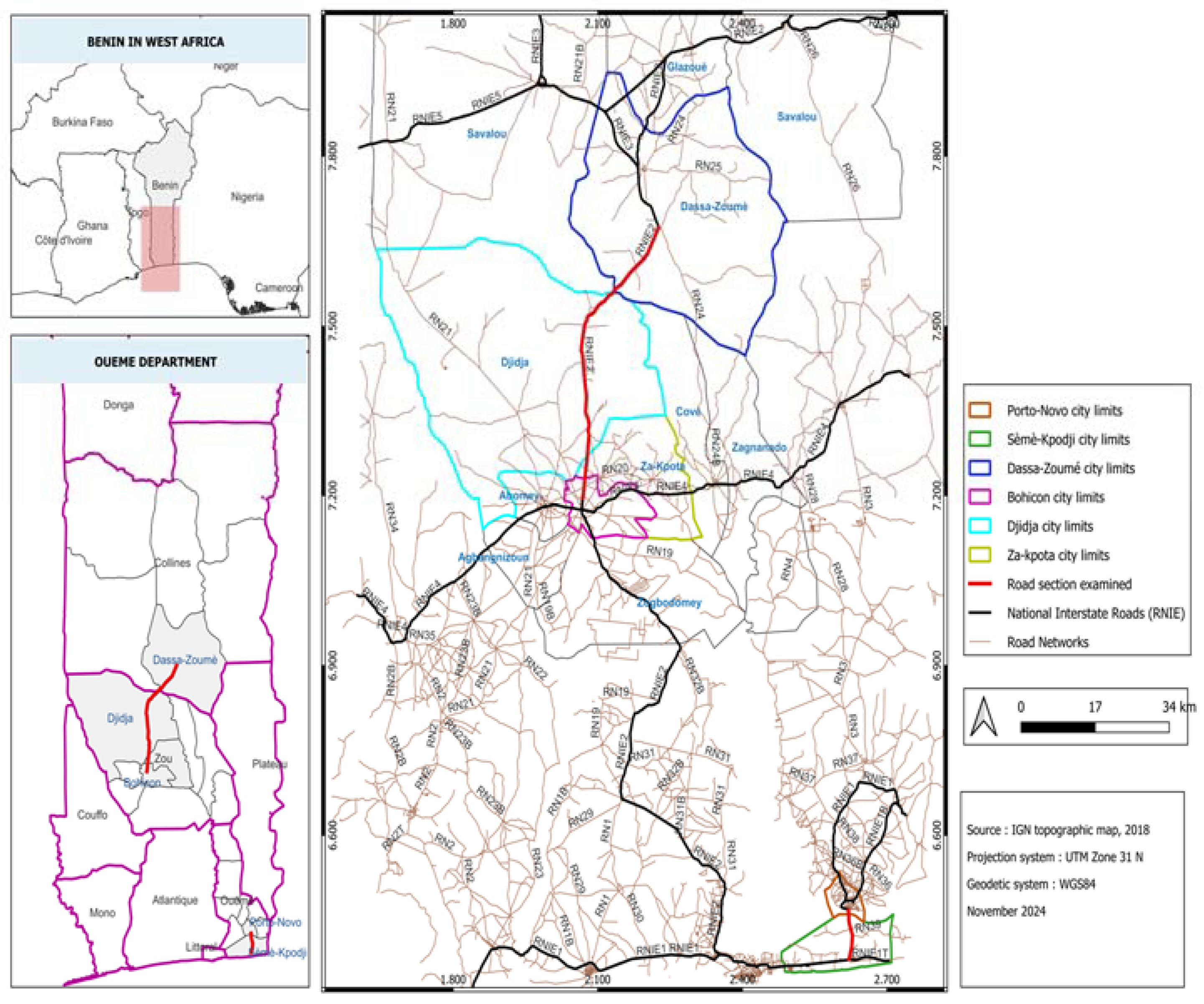
2.1. Collection of Data
2.2. Data Preprocessing
- Longitudinal cracks;
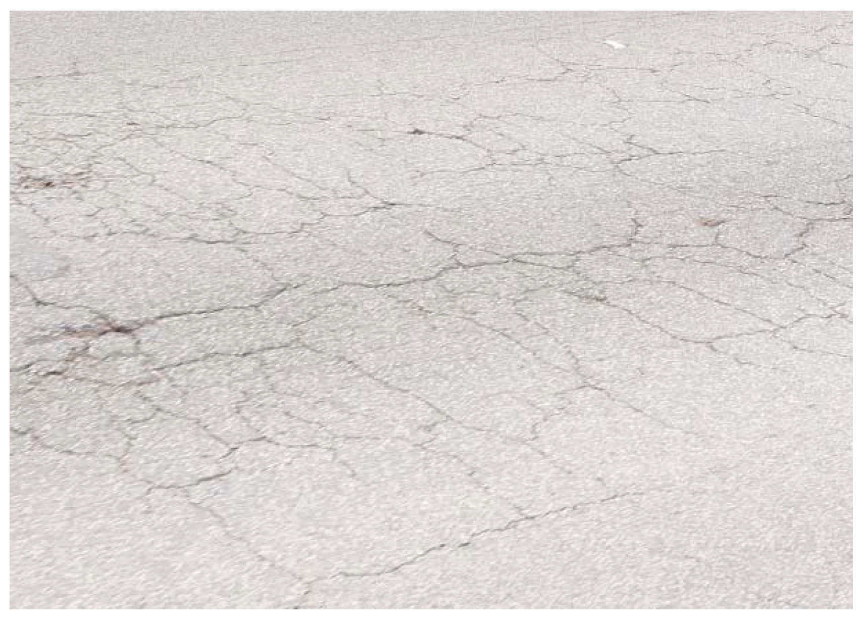
- Alligator cracks;
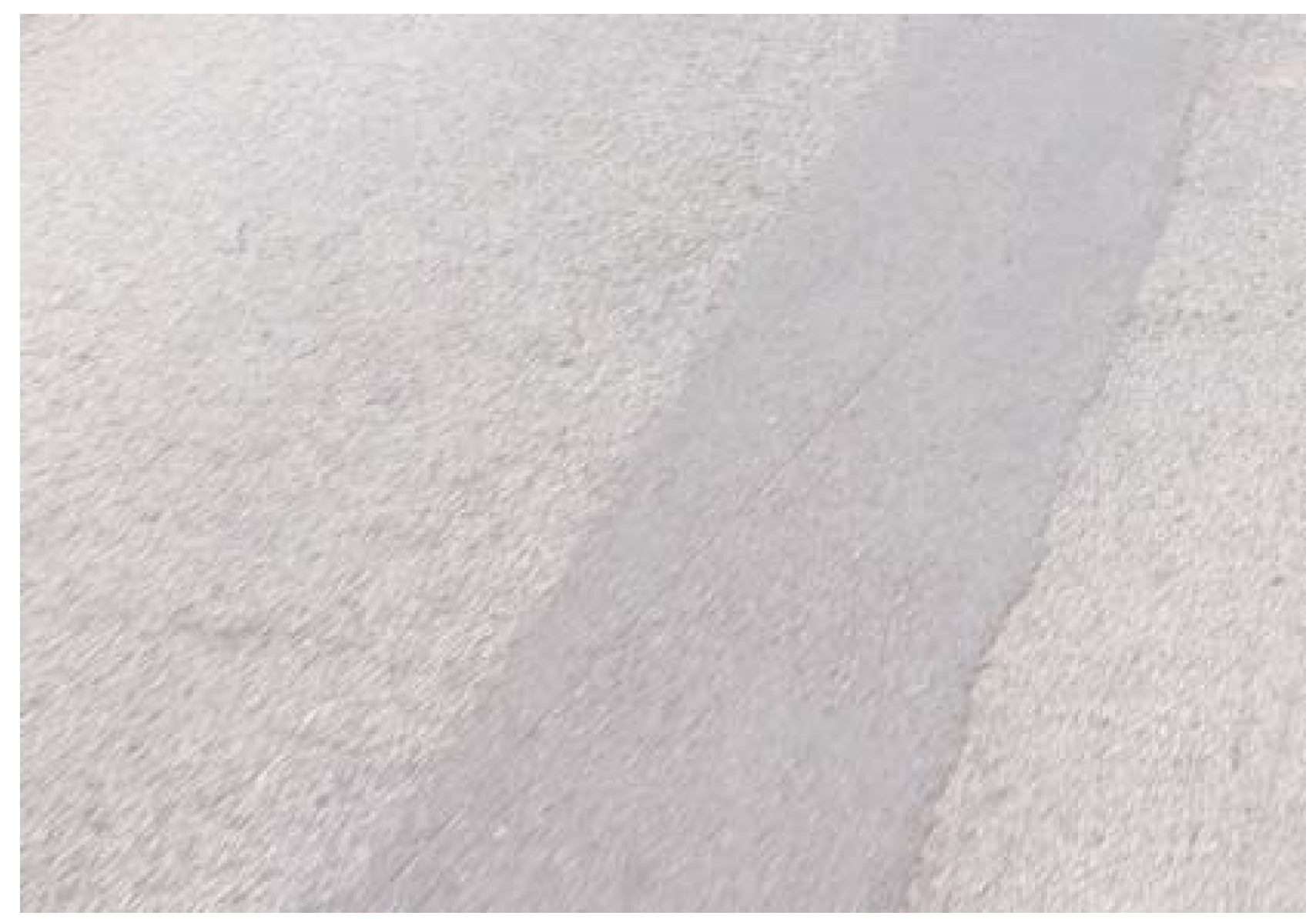
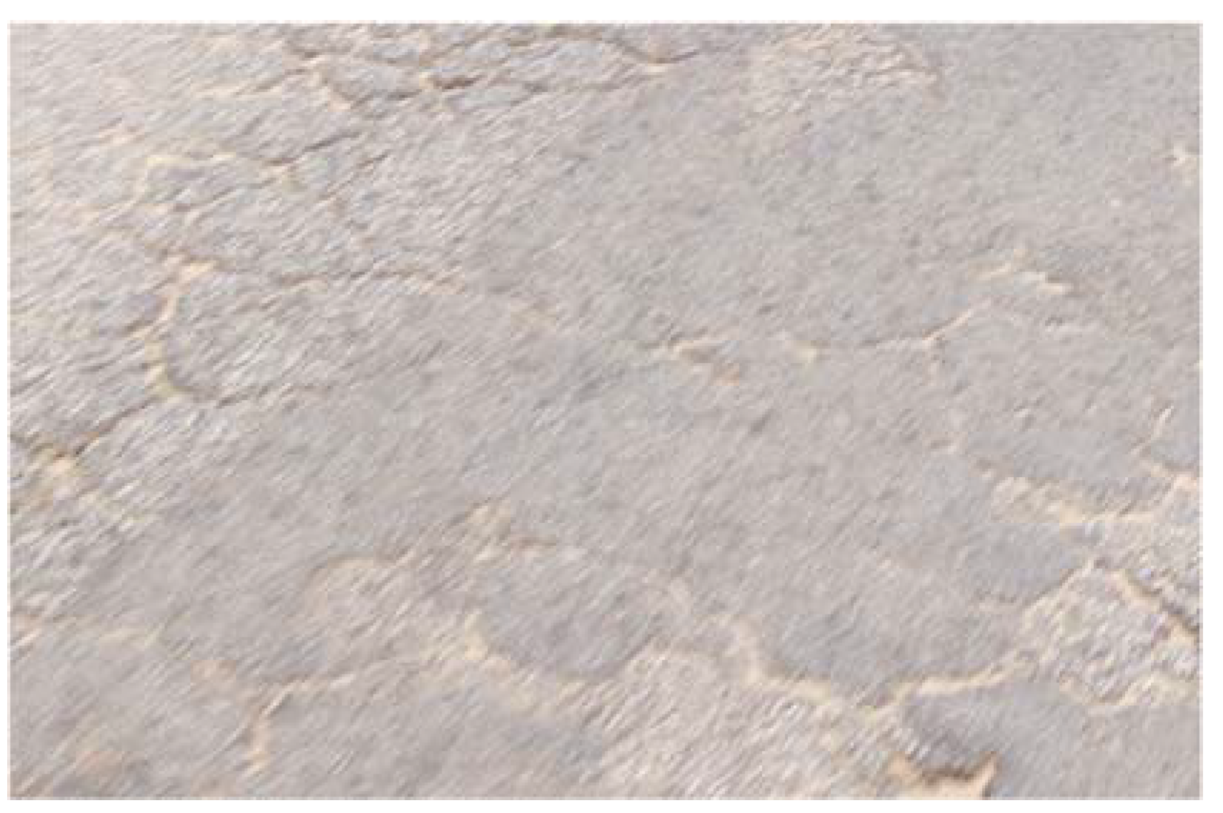
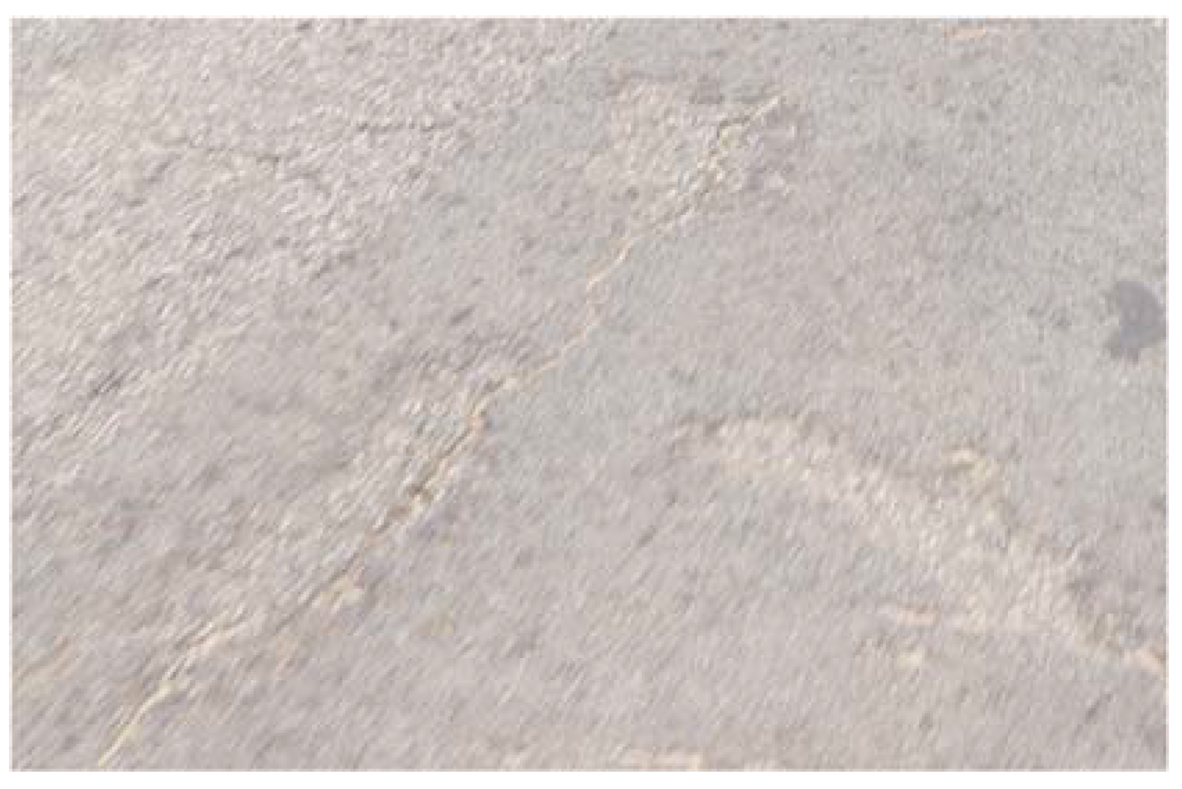
- Raveling;
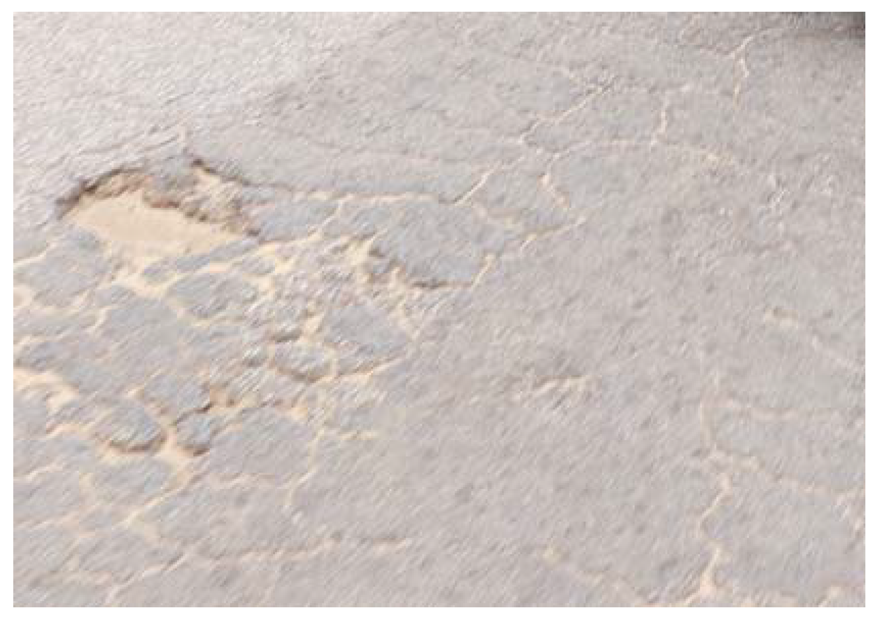
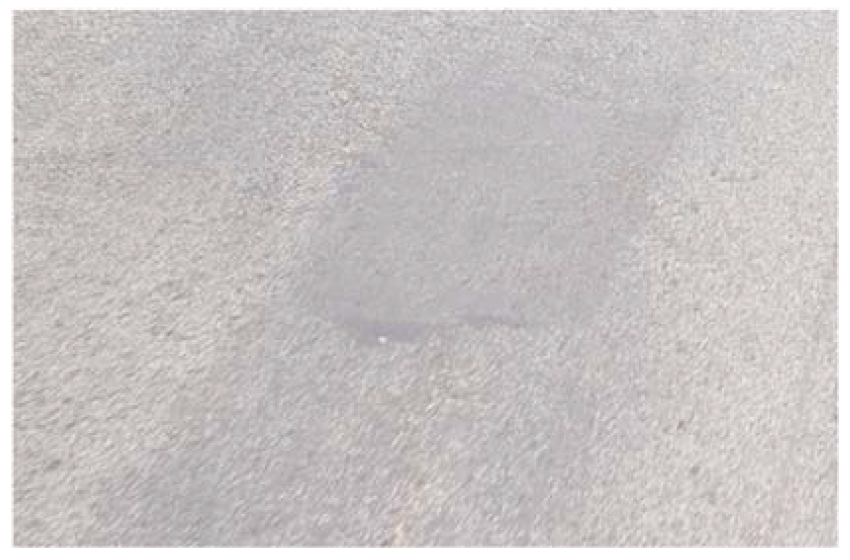
- Patching.
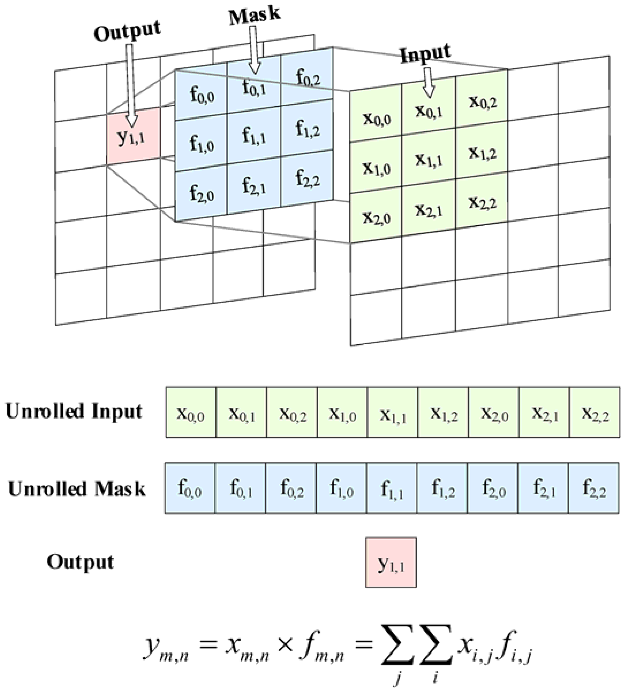
2.3. Development of Models
3. Results and Discussion
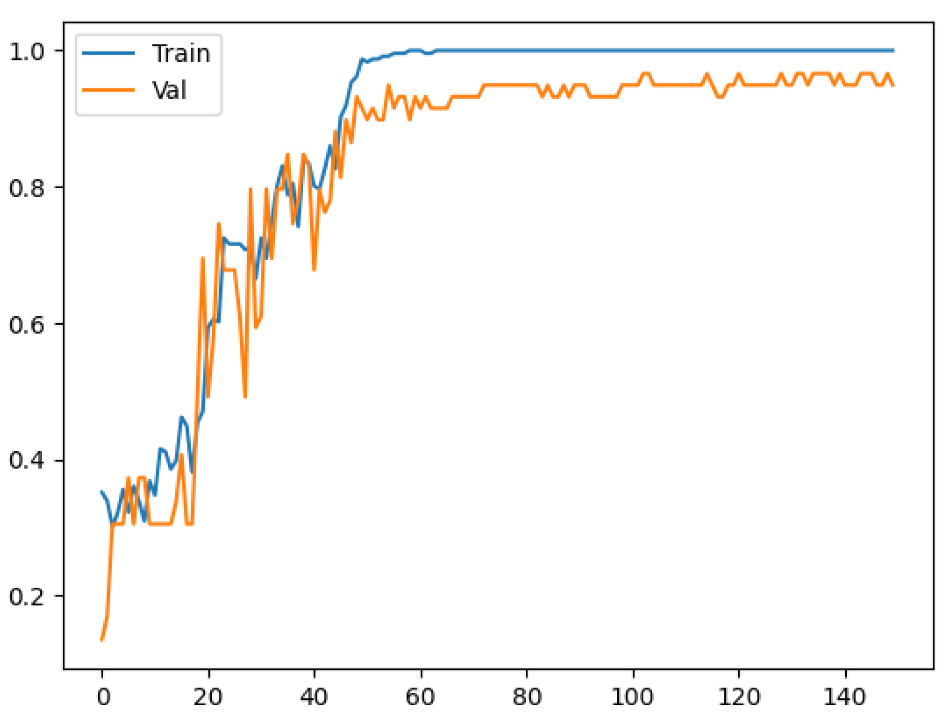
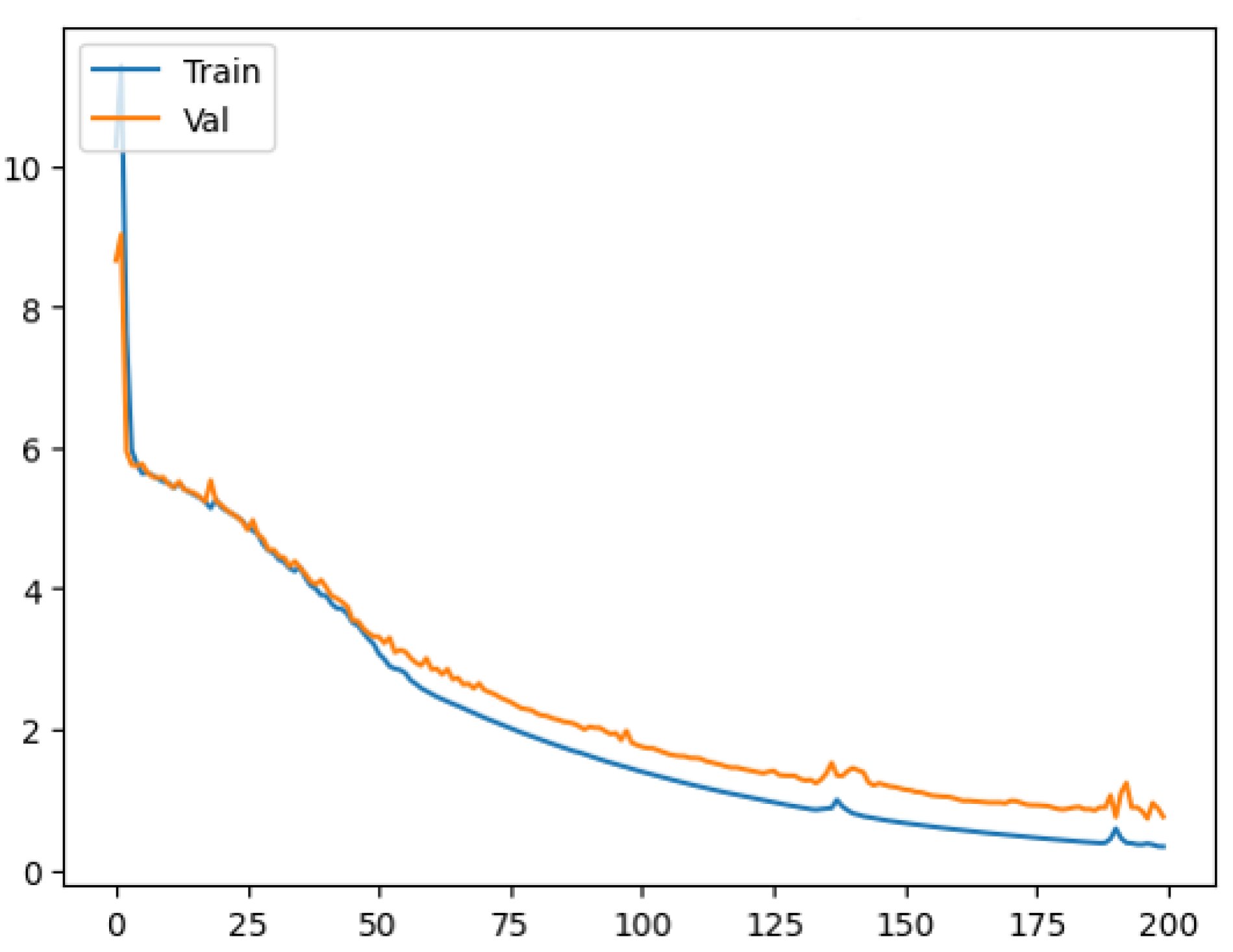
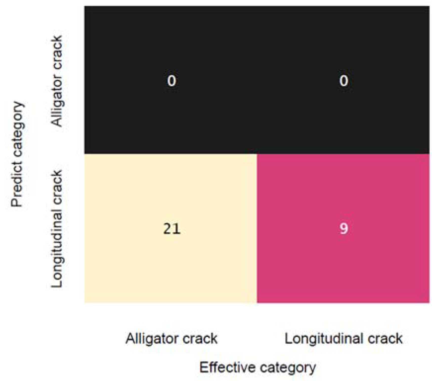
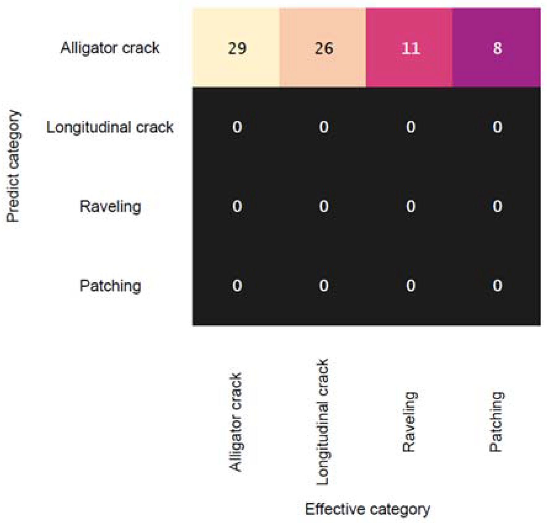
3.1. Model Training and Evaluation
3.2. Discussion and Model Performance Comparison
4. Conclusions
Author Contributions
Funding
Data Availability Statement
Acknowledgments
Conflicts of Interest
Abbreviations
| CNN | Convolutional Neural Network |
| VGG | Visual Geometry Group |
| ROA | Region Of Aggregation |
| ROB | Region Of Belief |
| LS-SVM | Least-Squares Support-Vector Machines |
| ANN | Artificial Neural Network |
References
- Ukhwah, E.N.; Yuniarno, E.M.; Suprapto, Y.K. Asphalt Pavement Pothole Detection Using Deep Learning Method Based on YOLO Neural Network. In Proceedings of the 2019 International Seminar on Intelligent Technology and Its Applications (ISITIA), Surabaya, Indonesia, 28–29 August 2019; pp. 35–40. [Google Scholar] [CrossRef]
- Hoang, N. Automatic Detection of Asphalt Pavement Raveling Using Image Texture Based Feature Extraction and Stochastic Gradient Descent Logistic Regression. Autom. Constr. 2019, 105, 102843. [Google Scholar] [CrossRef]
- CEBTP. LCPC Manuel Pour Le Renforcement Des Chaussées Souples En Pays Tropicaux; Documentation Française: Paris, France, 1985; ISBN 2.11.084817-0. [Google Scholar]
- IDRRIM. Diagnostic et Conception Des Renforcements de Chaussées; CEREMA, Ed.; Centre d’études et d’expertise sur les risques, l’environnement, la mobilité et l’aménagement (CEREMA): Paris, France, 2016; ISBN 978-2-37180-132-5. [Google Scholar]
- Zhang, C.; Nateghinia, E.; Miranda-Moreno, L.F.; Sun, L. Pavement Distress Detection Using Convolutional Neural Network (CNN): A Case Study in Montreal, Canada. Int. J. Transp. Sci. Technol. 2022, 11, 298–309. [Google Scholar] [CrossRef]
- Li, B.; Wang, K.C.P.; Zhang, A.; Yang, E.; Wang, G. Automatic Classification of Pavement Crack Using Deep Convolutional Neural Network. Int. J. Pavement Eng. 2020, 21, 457–463. [Google Scholar] [CrossRef]
- Zou, Q.; Cao, Y.; Li, Q.; Mao, Q.; Wang, S. CrackTree: Automatic Crack Detection from Pavement Images. Pattern Recognit. Lett. 2012, 33, 227–238. [Google Scholar] [CrossRef]
- Gopalakrishnan, K.; Khaitan, S.K.; Choudhary, A.; Agrawal, A. Deep Convolutional Neural Networks with Transfer Learning for Computer Vision-Based Data-Driven Pavement Distress Detection. Constr. Build. Mater. 2017, 157, 322–330. [Google Scholar] [CrossRef]
- Kirschke, K.R.; Velinsky, S.A. Histogram-Based Approach for Automated Pavement-Crack Sensing. J. Transp. Eng. 1992, 118, 700–710. [Google Scholar] [CrossRef]
- Oh, H.; Garrick, N.W.; Achenie, L. Segmentation Algorithm Using Iterative Clipping for Processing Noisy Pavement Images. In Imaging Technologies: Techniques and Applications in Civil Engineering; Second International ConferenceEngineering Foundation; Imaging Technologies Committee of the Technical Council on Computer Practices, American Society of Civil Engineers: Reston, VA, USA, 1998; pp. 148–159. [Google Scholar]
- Li, Q.; Liu, X. Novel Approach to Pavement Image Segmentation Based on Neighboring Difference Histogram Method. Congr. Image Signal Process. 2008, 2, 792–796. [Google Scholar] [CrossRef]
- Zhang, D.; Li, Q.; Chen, Y.; Cao, M.; He, L.; Zhang, B. An Efficient and Reliable Coarse-to-Fine Approach for Asphalt Pavement Crack Detection. Image Vis. Comput. 2017, 57, 130–146. [Google Scholar] [CrossRef]
- Yan, M.; Bo, S.; Xu, K.; He, Y. Pavement Crack Detection and Analysis for High-Grade Highway. In Proceedings of the 2007 8th International Conference on Electronic Measurement and Instruments, Xi’an, China, 16–18 August 2007; pp. 4548–4552. [Google Scholar] [CrossRef]
- Huidrom, L.; Kumar, L.; Sud, S.K. Method for Automated Assessment of Potholes, Cracks and Patches from Road Surface Video Clips. Procedia-Soc. Behav. Sci. 2013, 104, 312–321. [Google Scholar] [CrossRef]
- Kaseko, M.S.; Lo, Z.P.; Ritchie, S.G. Comparison of Traditional and Neural Classifiers for Pavement-Crack Detection. J. Transp. Eng. 1994, 120, 552–569. [Google Scholar] [CrossRef]
- Bray, J.; Verma, B.; Li, X.; He, W. A Neural Network Based Technique for Automatic Classification of Road Cracks. In Proceedings of the IEEE International Conference on Neural Networks—Conference Proceedings, Vancouver, BC, Canada, 16–21 July 2006; pp. 907–912. [Google Scholar]
- Hoang, N. An Artificial Intelligence Method for Asphalt Pavement Pothole Detection Using Least Squares Support Vector Machine and Neural Network with Steerable Filter-Based Feature Extraction. Adv. Civ. Eng. 2018, 2018, 7419058. [Google Scholar] [CrossRef]
- Munawar, H.S.; Hammad, A.W.A.; Haddad, A.; Soares, C.A.P.; Waller, S.T. Image-Based Crack Detection Methods: A Review. Infrastructures 2021, 6, 1–20. [Google Scholar] [CrossRef]
- Some, L. Automatic Image-Based Road Crack Detection Methods; Kth Royal Institute of Technologie: Stockholm, Sweden, 2016. [Google Scholar]
- Maeda, H.; Sekimoto, Y.; Seto, T.; Kashiyama, T.; Omata, H. Road Damage Detection and Classification Using Deep Neural Networks with Smartphone Images. Comput. Civ. Infrastruct. Eng. 2018, 33, 1127–1141. [Google Scholar] [CrossRef]
- Wang, D.; Liu, Z.; Gu, X.; Wu, W.; Chen, Y.; Wang, L. Automatic Detection of Pothole Distress in Asphalt Pavement Using Improved Convolutional Neural Networks. Remote Sens. 2022, 14, 3892. [Google Scholar] [CrossRef]
- Maslan, J.; Cicmanec, L. A System for the Automatic Detection and Evaluation of the Runway Surface Cracks Obtained by Unmanned Aerial Vehicle Imagery Using Deep Convolutional Neural Networks. Appl. Sci. 2023, 13, 6000. [Google Scholar] [CrossRef]
- Chun, P.J.; Yamane, T.; Tsuzuki, Y. Automatic Detection of Cracks in Asphalt Pavement Using Deep Learning to Overcome Weaknesses in Images and Gis Visualization. Appl. Sci. 2021, 11, 892. [Google Scholar] [CrossRef]
- Nhat-Duc, H.; Nguyen, Q.L.; Tran, V.D. Automatic Recognition of Asphalt Pavement Cracks Using Metaheuristic Optimized Edge Detection Algorithms and Convolution Neural Network. Autom. Constr. 2018, 94, 203–213. [Google Scholar] [CrossRef]
- Aggarwal, C.C. Neural Networks and Deep Learning; Springer International Publishing AG: Cham, Switzerland, 2018; ISBN 9783319944623. [Google Scholar]
- Aggarwal, C.C. Teaching Deep Learners to Generalize. In Neural Networks and Deep Learning; Springer International Publishing AG: Cham, Switzerland, 2018; pp. 169–216. ISBN 9783319944630. [Google Scholar]
- Aggarwal, C.C. Training Deep Neural Networks. In Neural Networks and Deep Learning; Springer International Publishing AG: Cham, Switzerland, 2018; pp. 105–167. ISBN 9783319944630. [Google Scholar]
- Hoang, N. Automatic Recognition of Asphalt Pavement Cracks Based on Image Processing and Machine Learning Approaches: A Comparative Study on Classifier Performance. Math. Probl. Eng. 2018, 2018, 6290498. [Google Scholar] [CrossRef]


| Class | ||||||
|---|---|---|---|---|---|---|
| Image Size | Alligator Crack | Longitudinal Crack | Raveling | Patching | Total | |
| Dataset 1 | 150 × 650 | 50 | 50 | 0 | 0 | 100 |
| Dataset 2 | 480 × 270 | 140 | 121 | 38 | 70 | 369 |
| Dataset 3 | 480 × 270 | 270 | 285 | 35 | 100 | 690 |
| Dataset 4 | 480 × 270 | 323 | 364 | 51 | 129 | 867 |
| Training Set | Validation Set | Test Set | Total | |
|---|---|---|---|---|
| Dataset 1 | 65 | 15 | 20 | 100 |
| Dataset 2 | 236 | 59 | 74 | 369 |
| Dataset 3 | 441 | 111 | 128 | 690 |
| Dataset 4 | 554 | 138 | 174 | 867 |
| Scenario 1 | Scenario 2 | Scenario 3 | Scenario 4 | Scenario 5 | Scenario 6 | Scenario 7 | Scenario 8 | |
|---|---|---|---|---|---|---|---|---|
| Epochs | 10 | 10 | 30 | 30 | 50 | 70 | 150 | 200 |
| Input shape | 150*650 | 150*650 | 270*480 | 270*480 | 270*480 | 270*480 | 270*480 | 270*480 |
| Layer Type | ||||||||
| Convolutional | 32 3*3 ReLU | 32 3*3 ReLU BN | 32 3*3 ReLU BN | 32 3*3 Leaky ReLU BN | 32 3*3 ELU | 32 3*3 ELU | 32 3*3 ELU | 32 3*3 ELU |
| Regularization | - | - | - | 16, l2 | 16, l2 | 16, l2 | 16, l2 | 16, l2 |
| Convolutional | 32 3*3 ReLU | 32 3*3 ReLU BN | 32 3*3 ReLU BN | 32 3*3 Leaky ReLU BN | 32 3*3 ELU | 32 3*3 ELU | 32 3*3 ELU | 32 3*3 ELU |
| Regularization | - | - | - | 16, l2 | 16, l2 | 16, l2 | 16, l2 | 16, l2 |
| MaxPooling | 2*2 | 2*2 | 2*2 | 2*2 | 2*2 | 2*2 | 2*2 | 2*2 |
| Regularization | 16, l2 | 16, l2 | 16, l2 | - | - | - | - | - |
| Convolutional | 64 3*3 ReLU | 64 3*3 ReLU BN | 64 3*3 ReLU BN | 64 3*3 Leaky ReLU BN | 64 3*3 ELU | 64 3*3 ELU | 64 3*3 ELU | 64 3*3 ELU |
| Regularization | - | - | - | 16, l2 | 16, l2 | 16, l2 | 16, l2 | 16, l2 |
| Convolutional | 64 3*3 ReLU | 64 3*3 ReLU BN | 64 3*3 ReLU BN | 64 3*3 Leaky ReLU BN | 64 3*3 ELU | 64 3*3 ELU | 64 3*3 ELU | 64 3*3 ELU |
| Regularization | - | - | - | 16, l2 | 16, l2 | 16, l2 | 16, l2 | 16, l2 |
| MaxPooling | 2*2 | 2*2 | 2*2 | 2*2 | 2*2 | 2*2 | 2*2 | 2*2 |
| Regularization | 16, l2 | 16, l2 | 16, l2 | - | - | - | - | - |
| Convolutional | 128 3*3 ReLU | 128 3*3 ReLU BN | 128 3*3 ReLU BN | 128 3*3 Leaky ReLU BN | 128 3*3 ELU | 128 3*3 ELU | 128 3*3 ELU | 128 3*3 ELU |
| Regularization | - | - | - | 16, l2 | 16, l2 | 16, l2 | 16, l2 | 16, l2 |
| Convolutional | 128 3*3 ReLU | 128 3*3 ReLU BN | 128 3*3 ReLU BN | 128 3*3 Leaky ReLU BN | 128 3*3 ELU | 128 3*3 ELU | 128 3*3 ELU | 128 3*3 ELU |
| Regularization | - | - | - | 16, l2 | 16, l2 | 16, l2 | 16, l2 | 16, l2 |
| MaxPooling | 2*2 | 2*2 | 2*2 | 2*2 | 2*2 | 2*2 | 2*2 | 2*2 |
| Regularization | 16, l2 | 16, l2 | 16, l2 | - | - | - | - | - |
| Convolutional | - | - | - | - | 256 3*3 ELU | 256 3*3 ELU | 256 3*3 ELU | 256 3*3 ELU |
| Regularization | - | - | - | - | 16, l2 | 16, l2 | 16, l2 | 16, l2 |
| Convolutional | - | - | - | - | 256 3*3 ELU | 256 3*3 ELU | 256 3*3 ELU | 256 3*3 ELU |
| Regularization | - | - | - | - | 16, l2 | 16, l2 | 16, l2 | 16, l2 |
| MaxPooling | - | - | - | - | 2*2 | 2*2 | 2*2 | 2*2 |
| Regularization | - | - | - | - | - | - | - | - |
| Convolutional | - | - | - | - | - | - | 512 3*3 ELU | 512 3*3 ELU |
| Regularization | - | - | - | - | - | - | 16, l2 | 16, l2 |
| Convolutional | - | - | - | - | - | - | 512 3*3 ELU | 512 3*3 ELU |
| Regularization | - | - | - | - | - | - | 16, l2 | 16, l2 |
| MaxPooling | - | - | - | - | - | - | 2*2 | 2*2 |
| Regularization | - | - | - | - | - | - | - | - |
| Flattening | ||||||||
| Fully connected | 256 ReLU | 256 ReLU | 512 ReLU | 512 ReLU | 512 ELU | 512 ELU | 512 ELU | 512 ELU |
| Dropout | 0.5 | 0.5 | 0.5 | 0.3 | 0.3 | 0.3 | 0.3 | 0.4 |
| Output | 2 Softmax | 2 Softmax | 4 Softmax | 4 Softmax | 4 Softmax | 4 Softmax | 4 Softmax | 4 Softmax |
| Scenario 1 | Scenario 2 | Scenario 3 | Scenario 4 | Scenario 5 | Scenario 6 | Scenario 7 | Scenario 8 | |
|---|---|---|---|---|---|---|---|---|
| Accuracy | 43.3% | 36.7% | 36.0% | 39.2% | 62.2% | 86.5% | 94.6% | 95.9% |
| Loss | 3.49 | 2.35 | 3.18 | 1.61 | 2.26 | 1.86 | 2.70 | 2.46 |
Disclaimer/Publisher’s Note: The statements, opinions and data contained in all publications are solely those of the individual author(s) and contributor(s) and not of MDPI and/or the editor(s). MDPI and/or the editor(s) disclaim responsibility for any injury to people or property resulting from any ideas, methods, instructions or products referred to in the content. |
© 2025 by the authors. Licensee MDPI, Basel, Switzerland. This article is an open access article distributed under the terms and conditions of the Creative Commons Attribution (CC BY) license (https://creativecommons.org/licenses/by/4.0/).
Share and Cite
Yabi, C.P.; Gbehoun, G.F.; Tamou, B.C.K.; Alamou, E.; Gibigaye, M.; Farsangi, E.N. Analysis and Classification of Distress on Flexible Pavements Using Convolutional Neural Networks: A Case Study in Benin Republic. Infrastructures 2025, 10, 111. https://doi.org/10.3390/infrastructures10050111
Yabi CP, Gbehoun GF, Tamou BCK, Alamou E, Gibigaye M, Farsangi EN. Analysis and Classification of Distress on Flexible Pavements Using Convolutional Neural Networks: A Case Study in Benin Republic. Infrastructures. 2025; 10(5):111. https://doi.org/10.3390/infrastructures10050111
Chicago/Turabian StyleYabi, Crespin Prudence, Godfree F. Gbehoun, Bio Chéissou Koto Tamou, Eric Alamou, Mohamed Gibigaye, and Ehsan Noroozinejad Farsangi. 2025. "Analysis and Classification of Distress on Flexible Pavements Using Convolutional Neural Networks: A Case Study in Benin Republic" Infrastructures 10, no. 5: 111. https://doi.org/10.3390/infrastructures10050111
APA StyleYabi, C. P., Gbehoun, G. F., Tamou, B. C. K., Alamou, E., Gibigaye, M., & Farsangi, E. N. (2025). Analysis and Classification of Distress on Flexible Pavements Using Convolutional Neural Networks: A Case Study in Benin Republic. Infrastructures, 10(5), 111. https://doi.org/10.3390/infrastructures10050111