The Effect of Girder Profiles on the Probability of Fatigue Damage in Continuous I-Multigirder Steel Bridges

Abstract

Fatigue is one of the main sources of mechanical failure in steel bridges. However, a few studies have investigated the relationship between the longitudinal shape of bridge girders and long-term fatigue effects. This paper shows how different girder profiles affect the probability of fatigue damage occurring in continuous I-multigirder steel bridges. The analysis was conducted using realistic traffic scenarios defined through truck data collected in USA and Canada. Monte Carlo simulations with 5000 realizations were performed on several continuous bridge configurations with different span lengths and different girder profiles. The results of the analysis showed that the probability of fatigue damage is affected by profile shape and the smoothness of the transition between the maximum and minimum height of the cross section. In particular, the probability of fatigue damage on continuous I-multigirder steel bridges can be reduced by up to 26% for typical fatigue construction details over a bridge service life of 75 years by modifying the geometry of the girders during the design phase of the bridge.

1. Introduction

Stress accumulation under low-intensity high-frequency conditions, or fatigue, due to highway traffic load is one of the main concerns for typical highway steel bridges that may lead to major failure events [1,2,3,4]. Researchers have studied fatigue since the nineteenth century as one of the main sources of mechanical failures of steel structures [5]. Fatigue has a direct effect on structural safety and durability, for which different traffic load conditions contribute to different fatigue scenarios [6]. The same is true for other parameters such as environmental conditions and material degradation [7].

The stress history of bridge members is a random phenomenon, and the fatigue life is dependent on the truck traffic flow over the bridges [8,9,10]. For steel members, the accumulation of fatigue is determined by two main parameters: the stress range and its number of cycles [10,11]. A thorough bridge fatigue analysis should be conducted by analyzing actual traffic load time-histories [10,12]. Collecting a representative sample size of the traffic loads is a crucial factor to determine stress time histories for the analysis of bridge fatigue damages. To overcome such a difficulty, in recent decades, structural health monitoring systems (SHMs) have been developed to collect realistic time-dependent load data on bridges. Stress–strain time histories for probabilistic fatigue investigations are currently collected by bridge weigh-in-motion (BWIM) methods [13,14,15,16] or through strain gauges installed on bridge members [17,18]. When investigating fatigue damage from field stress data, several authors have shown that a bilinear fatigue model provides more accurate results compared to the traditionally used models that include constant amplitude fatigue thresholds (CAFTs) [19,20,21]. However, SHM systems are currently only implemented on a limited number of bridges compared to the entire population, which, excluding culverts, consists of 524,400 bridges in the United States and Canada [22,23].

As an alternative to installing SHM systems on bridges, engineers can collect pertinent traffic data from monitoring devices such as road pavement weigh-in-motion (WIM) systems that have been installed at many locations across the United States and Canada. These provide representative traffic data on bridges within their proximity. Specifically, the Long-Term Pavement Performance (LTPP) program of the Federal Highway Administration (FHWA) collects vehicle data, including axle weight and axle spacings from 570 WIM sites in the United States and Canada that can be used for assessing the safety of bridges under cyclic and extreme loading [24,25,26,27,28,29,30,31]. The LTTP program is part of the long-term infrastructure performance program (LTIP) sponsored by the Federal Highway Administration in the United States. The LTIP envelopes both the long-term bridge (LTBP) and the pavement performance program [22,32].

WIM data have also been extensively used in past studies to assess the probability of bridge superstructure failures due to overloading events [24,25,27,28,29,31,33,34,35,36]. Similarly, researchers have also used field traffic data to develop probabilistic fatigue damage models [1,11,16,19,21,37,38,39,40,41,42,43,44,45,46,47,48,49,50,51,52,53,54]. Most of the probabilistic analyses of bridge fatigue were initially based on the experimental results of Fisher et al. [55,56]. Schilling [11] has shown how a complex stress history can cause more fatigue damage to bridge girders than estimated by the then commonly used simplified approximation of the maximum stress range. A similar conclusion was reached by Dexter et al. [57] who demonstrated that Miner’s rule [58] provides an appropriate approach to characterizing truck loading effects. This was achieved by performing the variable-amplitude fatigue testing of various bridge components. The same authors also indicated that a significant proportion of cracking in steel bridges is due to out-of-plane distortions in web gaps at connection plates for cross frames, diaphragms, or floor beams. However, according to McConnell and Almoosi [59], who recently investigated this phenomenon through field evaluation, distortion-induced fatigue is more likely when side-by-side truck events occur. However, side-by-side events are less frequent than single-lane loading events, which dominate bridge fatigue cracking. According to [24,60], side-by-side truck crossings take place only with a probability on the order of 2–5% in typical bridges with Average Daily Truck Traffic (ADTT) in the range of 1500 to 2000 trucks per day.

Furthermore, the stress ranges and fatigue of bridge members are not only functions of the load history but also functions of the longitudinal profile of the girders, even when bridges are subjected to the same load history. To the best of the authors’ knowledge, no previous studies have investigated the effect of girder profiles on the reliability of bridges for fatigue. Therefore, the objective of this paper is to investigate how the longitudinal shape of girders coupled with realistic truck traffic scenarios affect the probability of fatigue damage occurring in continuous I-multigirder steel bridges. To achieve this objective, a Monte Carlo simulation approach is used to characterize the response of bridges with different girder profiles under the same truck population. The Monte Carlo simulation was chosen because of its flexibility to be applied to complex loading and structural configurations. Then, a reliability analysis was performed on the limit state function used to calibrate the AASHTO LRFD fatigue truck model [40]. Traffic profiles were built using the aforementioned traffic data collected in the United States and Canada from 2012 with weigh-in-motion (WIM) systems from the LTPP program.

The remaining part of the manuscript describes the methodology used in this study to characterize bridge characteristics, traffic data, the models to compute fatigue stresses and fatigue damage on bridge girders, and the reliability analysis for fatigue. In the last part of the paper, a discussion of the results and conclusions is presented.

2. Materials and Methods

2.1. Characterization of Bridges

Bridge data were extracted from the FHWA long-term bridge performance program (LTBP) and the Infrastructure Canada databases [22,23]. According to these sources, excluding culverts, there are about 475,000 bridges in the USA and 49,400 bridges in Canada. The focus of the analysis was concentrated on continuous steel bridges because the accumulation of fatigue damage on this bridge type is higher than simply supported bridges due to the multiple load paths generated while a truck crosses a bridge [61]. Also, box girders were not considered because of the limited number of this bridge type in the inventory, which only accounts for 1.5% of the highway continuous steel bridge population [22]. Many of continuous I-multigirder steel bridges in the United States and Canada have a variable longitudinal profile, as shown in Figure 1. These profiles can have either a linear or a parabolic shape. The ratio between the maximum and minimum depth of the cross section ranges between 1.4 and 1.6 based on the image processing of a set of photographs collected from bridges on interstate and regional roads. These aspect ratios are also in agreement with the recommendations of FHWA for variable steel girder profiles, which limit the value of the aspect ratio to 2.0 [62]. The transition point between the prismatic and variable cross section along the girder is generally dictated by engineering judgment and construction requirements rather than a mechanical behaviour. Accordingly, the ratio between the length of the variable portion of the girder cross section and one half of the span length, herein defined as $\rho$, can be as small as 20%, as shown in Figure 2. The representation of $\rho$ is schematically shown in the profiles depicted in Figure 3 for bridges with linear and parabolic shapes.

2.2. Representative Bridge Sample

Regarding the span configuration, about 5%, or 23,750, of the total bridge population were found to be continuous steel I-multigirder bridges. According to LTBP data, 23,604 of these have less than 20 spans and about 86.2% of the 23,604 bridges have less than 5 spans. A further analysis showed that for the 5759 two-span bridges, the maximum span length ranged between 7.0 m and 110.0 m, with about 96.7% (or 5567) of the bridges having a maximum span length less than 65.0 m. For most two-span bridges, the ratio between the maximum span length and the total bridge length ($\lambda$) ranges between 0.35 and 0.55.

Similar statistics were collected for three-span and four-span bridges. For three-span continuous steel bridges, about 97.5% (or 10,039) have a maximum span length less than 80.0 m, while the maximum span ratio $\lambda$ ranges between 0.25 and 0.45. Finally, for four-span continuous bridges, about 96.3% (or 4138) of the 4298 bridges have a maximum span length shorter than 70.0 m, and the maximum span length ratio ranges between 0.25 and 0.35.

According to these statistics, bridge span lengths from 10.0 m to 50.0 m and maximum span–bridge length ratios from 0.25 to 0.50 were considered for the numerical simulations. In addition, a girder spacing of 2.4 m was used for the analysis. The choice of a single value for the girder spacing does not undermine the validity of the study because the focus is on the effect on the longitudinal girder profile once the desired spacing for a bridge is chosen. The number of longitudinal girders was set as equal to 5, which is typical for redundant highway bridges [63]. These configurations accommodate between two and three lanes of traffic. A composite concrete deck 250 mm thick was used to connect the steel girders with a constant 1.0 m overhang on both sides from the exterior girders. Two aspect ratios between the maximum and minimum cross-section depth equal to 1.4 and 1.6 were considered. For each of these configurations, either a linear (L) or a parabolic (P) profile was analyzed. As a reminder, these profiles are schematically shown in Figure 3. Finally, four different $\rho$ values, equal to 25.0%, 50.0%, 75.0%, and 100%, were analyzed. The bridge parameters are listed in

Table 1. Continuous bridge configurations analyzed.

Bridge N.	N. Spans	Shape	$\mathit{\rho }$ [%]	Spacing [m]	Spans [m]	Girder Flange		Girder Web
						Width [mm]	Thickness [mm]	Variable Depth [mm]	Thickness [mm]
1	2	L, P	25–100	2.4	10-10	550	30	400–640	4
2					10-17	440	25	680–1088	6
3					20-20	470	25	800–1280	8
4					20-33	550	26	1320–2110	10
5					33-33	550	26	1320–2110	10
6					50-30	750	40	2000–3200	15
7					50-50	750	40	2000–3200	15
8	3	L, P	25–100	2.4	10-10-10	550	29	400–640	4
9					10-17-10	440	24	680–1088	6
10					33-33-33	530	27	1320–2110	10
11					30-50-30	750	40	2000–3200	15
12					50-50-50	750	40	2000–3200	15
13	4	L, P	25–100	2.4	25-25-25-25	485	27	1000–1600	8
14					50-50-50-50	750	40	2000–3200	15

. The parameters listed in Table 1 are representative of about 83.1% of the continuous steel I-multigirder bridges in the inventory. The combination of these parameters resulted in a total of 224 different bridge configurations.

For each span configuration, the dimensions of the steel girders were estimated using empirical equations calibrated based on the design of highway bridges according to the AASHTO specifications [34]. For the bridges listed in Table 1, the minimum height of the cross section was set equal to ${\displaystyle \frac{{\mathrm{L}}_{\max }}{25}}$ [62,64]. The dimensions of the cross sections obtained from the empirical equations were found to be consistent with actual girder dimensions of similar bridges constructed in Manitoba following the AASHTO specifications [65].

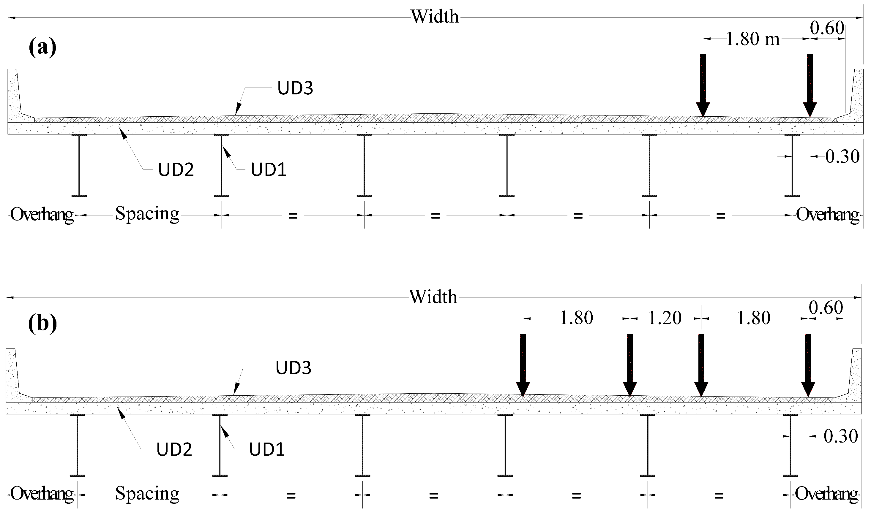
2.3. Characterization of Truck Configurations

The statistical characterization of truck loads and truck configurations was completed using WIM data from the LTPP program [32]. The WIM data collection of the LTPP program reached its peak between 2008 and 2012, with an average of 3350 WIM files collected every year from local and state agencies according to the latest traffic monitoring guide (TMG-W) data format [66]. These files are publicly available through the LTPP website [32]. In this study, the entire set of WIM files for the 2012 was analyzed because it provided the largest spatial distribution of data collected at WIM locations for a single year, as shown in Figure 4. As a result, this provides a representative picture of the entire truck population in the United States and Canada.

The classification of the 66.8 million trucks from the 2012 database into FHWA categories [66] showed that 71.2% were five-axle Class 9 tractor-trailers and 15.2% were two axle Class 5 single-unit trucks, as shown in the third column of

Table 2. GVW distribution parameters for different truck configurations.

Class (1)	N. Axles (2)	Proportion [%] (3)	Distribution (4)	Parameters		${\mathit{\chi }}^2$ Value (7)
				${\mathit{p}}_{\mathbf{1}}$ (5)	${\mathit{p}}_{\mathbf{2}}$ (6)
5	2	15.2	Log-normal	4.2	0.3	31.37
6	3	5.0	Log-normal	4.8	0.4	8.70
8	4	4.0	Log-normal	4.9	0.3	23.75
9	5	71.2	Truncated-normal	243.4	77.3	73.96
10	6	2.2	Log-normal	5.45	0.36	82.97
13	8	1.3	Truncated-normal	426.6	123.5	541.21

. The next most frequent truck type was the single-unit truck with three axles (Class 6) that accounted for 5.0% of the total population, followed by tractor-trailers with four axles (Class 8) (4.0%), tractor-trailers with six axles (Class 10) (2.2%), and long-hauling double trailer trucks with eight axles (Class 13) (1.3%). These six truck configurations accounted for 98.9% of the entire LTPP truck population in 2012.

A subsequent analysis of these six truck categories revealed the distributions of gross vehicle weight (GVW), the axle weight to GVW ratio, and axle spacings. The histograms of the GVW for each truck category are shown in Figure 5.

Table 2 shows the parameters of the statistical distributions that best fit the GVW data expressed in kN in each truck group.

Column five of Table 2 indicates either the mean value ($p_1$) of the data modelled using a normal distribution (truncated at zero) or the log-mean for the log-normal distribution. Column six of Table 2 lists the standard deviation ($p_2$), while column seven of table indicates the chi-square value of the goodness of fit test for each distribution. The reference chi-square value with 97 degrees of freedom at a 95% confidence level is 75.28. A chi-square value below 75.28 indicates a very good fit for the data. Based on the values listed in Table 2, the models fit the GVW data well, except for Class 13. This is due to the multi-modal behaviour exhibited by the gross weights in this category. However, given the small proportion of this class compared to the entire population, a slight error in the estimate of the gross weight based on the proposed model in this category will not compromise the accuracy of the structural reliability analysis, which will be discussed later.

A statistical analysis of the axle weight to GVW ratios was also performed for each truck category. These ratios are assumed to be normally distributed based on past investigations [67]. The results of this analysis are summarized in

Table 3. Axle weight to GVW ratio statistics.

Class	Parameter	Truck Axle
		1	2	3	4	5	6	7	8
5	Mean	0.42	0.58	-	-	-	-	-	-
	COV	0.19	0.14	-	-	-	-	-	-
6	Mean	0.41	0.30	0.29	-	-	-	-	-
	COV	0.26	0.21	0.21	-	-	-	-	-
8	Mean	0.25	0.35	0.20	0.20	-	-	-	-
	COV	0.24	0.27	0.28	0.32	-	-	-	-
9	Mean	0.21	0.21	0.20	0.19	0.19	-	-	-
	COV	0.32	0.11	0.11	0.18	0.19	-	-	-
10	Mean	0.20	0.19	0.19	0.14	0.14	0.14	-	-
	COV	0.32	0.12	0.12	0.24	0.20	0.24	-	-
13	Mean	0.12	0.11	0.15	0.14	0.12	0.13	0.12	0.11
	COV	0.40	0.30	0.14	0.20	0.20	0.19	0.20	0.22

.

The values listed in Table 3 show the mean and the coefficient of variation (COV) of each axle weight to GVW ratio. For semi-trailers, it is common to use a fixed value for the steering wheel, which is fairly consistently equal to 35.0 kN, and then divide the rest of the weight by the rest of the axles following a statistical distribution. For Class 13 trucks, the COV of 0.40 for the steering axle load is due to the large variation in the GVW in Class 13 trucks.

Statistics of truck axle spacings were also investigated for each FHWA class. The mean and COV for each axle spacing are summarized in

Table 4. Axle spacings statistics.

Class	Parameter	Axle Spacing
		1–2	2–3	3–4	4–5	5–6	6–7	7–8
5	Mean [m]	5.0	-	-	-	-	-	-
	COV	0.22	-	-	-	-	-	-
6	Mean [m]	5.3	1.3	-	-	-	-	-
	COV	0.15	0.08	-	-	-	-	-
8	Mean [m]	4.5	7.2	2.3	-	-	-	-
	COV	0.20	0.44	1.17	-	-	-	-
9	Mean [m]	5.1	1.3	9.8	1.4	-	-	-
	COV	0.14	0.31	0.11	0.43	-	-	-
10	Mean [m]	5.1	1.3	9.1	1.4	1.5	-	-
	COV	0.14	0.08	0.18	0.21	0.20	-	-
13	Mean [m]	4.2	1.6	3.7	5.3	2.4	3.5	1.7
	COV	0.21	0.25	0.76	0.74	0.83	0.66	0.71

. The axle spacings are also assumed to be normally distributed [67]. The parameters listed in Table 2, Table 3 and Table 4 were used to simulate the truck load characteristics for the structural analysis.

2.4. Structural Analysis

The procedure to compute the mechanical response of bridges is illustrated using the example shown in Figure 6, which depicts a two-span continuous bridge system with a composite concrete deck over steel I-multigirders.

For each girder cross section at position $P(x,y)$, a stress tensor $\mathbf{\sigma }$ is computed at each value of the z coordinate along the depth of the cross section A-A as the input truck with parameters contained in the vector ${\mathbf{\psi }}_i$ travels over the bridge, as shown in Figure 6, where $i=\left[1,\dots ,N_T\right]$ and $N_T$ is the total number of truck configurations investigated. Given the bending behaviour of composite steel girders, the stress tensor $\mathbf{\sigma }$ is characterized by an axial component ${\sigma }_x$ and a shear stress ${\tau }_{x,z}={\tau }_{z,x}=\tau$ component. The stress tensor’s history is recorded for every longitudinal position $x_{{\psi }_i}$ of the truck ${\mathbf{\psi }}_i$ as it travels over the bridge. Note that $x_{{\psi }_i}$ should not be confused with the location x of P, as shown in Figure 6. The stress tensor in the global reference system XYZ is then converted into principal components according to Mohr’s equations [68]:

$$\begin{array}{cc}\hfill tan\left(2\alpha \right)& ={\displaystyle \frac{\tau }{{\sigma }_x}}\hfill \end{array}$$

(1)

$$\begin{array}{cc}\hfill {\sigma }_I& ={\displaystyle \frac{{\sigma }_x}{2}}+\sqrt{{\left({\displaystyle \frac{{\sigma }_x}{2}}\right)}^2+{\tau }^2}\hfill \end{array}$$

(2)

$$\begin{array}{cc}\hfill {\sigma }_{II}& ={\displaystyle \frac{{\sigma }_x}{2}}-\sqrt{{\left({\displaystyle \frac{{\sigma }_x}{2}}\right)}^2+{\tau }^2}\hfill \end{array}$$

(3)

where $\alpha$ is the angle of rotation of the principal axes relative to the global X axis and ${\sigma }_I$ and ${\sigma }_{II}$ are the major and minor components of the principal stresses, respectively. This is also schematically shown in Figure 6.

The bridges are modelled as a grillage using an efficient simulation framework named OpenBRAIN [34]. This framework performs the linear and nonlinear structural analysis of girder-type bridges using OpenSees as the back engine for the structural analysis [69]. For a given bridge configuration, OpenBRAIN performs the analysis of hundreds of load configurations on a structure in a matter of seconds thanks to its parallel implementation, making this software extremely efficient when conducting Monte Carlo simulations.

OpenBRAIN creates a grillage consisting of main girders oriented along the x direction of a Cartesian reference system, connected by the deck in the y direction. Each girder is divided into elements with an approximate length of 0.5 m in the longitudinal direction, and, at each joint, the girders are connected by transverse beams simulating the deck in the perpendicular direction. Permanent and live loads are applied in the z direction, which is normal to the plane of the bridge. Deck elements are discretized uniformly along the span length and modelled as unidirectional slab strips. Provided a set of parameters, such as a number of spans, vector of span lengths, and overall deck width, in addition to the dimensions and material properties of the deck and girders, OpenBRAIN calculates each member’s moment–curvature relationship. The composite moment curvature relationship of the girders is computed by dividing the cross section of each grillage beam into fibres and calculating the moment value that satisfies the condition of equilibrium of all fibres for each value of the curvature, $\chi$. The stress–strain relationship $\sigma$-$ϵ$ for concrete in compression is described by the Ramberg–Osgood model given in Equation (4) [70], neglecting the contribution of concrete in tension. The stress–strain relationship for reinforcing steel is given in Equation (5) [71]. The value of concrete strengths $f_c^{\prime }$ for regular concrete was set equal to 35.0, while the plate girders and reinforcing steel yielding stress $f_y$, respectively, 350 MPa and 410 MPa. The reinforcement area in the concrete deck was set equal to 0.8% of the top and bottom of the concrete deck area. Further details on the modelling processes of the I-girder bridges are provided in [34,36,67]. A similar approach is also used in OpenBRAIN to calculate the non-composite ultimate capacity when bending the deck elements.

$$\begin{array}{c}\hfill \sigma \end{array}=\left\{\begin{array}{c}{f}_c^{\prime }\left[{\displaystyle \frac{2·ϵ}{{ϵ}_0}}-{\left({\displaystyle \frac{ϵ}{{ϵ}_0}}\right)}^2\right];ϵ\le {ϵ}_0;{ϵ}_0=1.8{\displaystyle \frac{f_c^{\prime }}{E_c}}\hfill \\ f_c^{\prime }-0.15f_c^{\prime }{\left({\displaystyle \frac{ϵ-{ϵ}_0}{0.003-{ϵ}_0}}\right)}^2;ϵ>{ϵ}_0;E_c=4700\sqrt{f_c^{\prime }}\left[\mathrm{MPa}\right]\hfill \end{array}\right.$$

(4)

$$\begin{array}{c}\hfill \sigma \end{array}=\left\{\begin{array}{c}{E}_s·ϵ;ϵ\le {ϵ}_y={\displaystyle \frac{f_y}{E_s}};E_s=200,000\left[\mathrm{MPa}\right]\hfill \\ f_y;{ϵ}_y<ϵ\le {ϵ}_h;{ϵ}_h=10·{ϵ}_y\hfill \\ f_u-\left(f_u-f_y\right){\left({\displaystyle \frac{{ϵ}_u-ϵ}{{ϵ}_u-{ϵ}_h}}\right)}^2;{ϵ}_h<ϵ\le {ϵ}_u;f_u=1.5·f_y\hfill \end{array}\right.$$

(5)

As an example, Figure 7 shows the mesh discretization for a continuous bridge configuration analyzed in this study. The bridge has two spans, which are 20.0 m long. In this example, the number of girders is equal to five, spaced at 2.6 m. For the finite element analysis of the grillage, each span was divided into 50 sections. Figure 7 also shows the vertical displacement of the bridge when it is loaded by a two-axle truck with a total length of 4.0 m and a gross weight of 236 kN. The location of the truck on the bridge is with the centroid of the axle weights at the midspan on the left span close to the southern girder.

For each bridge configuration with a specified number of girders, the bending and shear on each girder are computed using Courbon’s distribution factor ($DF$) [72]. Courbon’s distribution factor assumes that the lateral profile of the bridge cross section is not distorted after deformation. This assumption is fairly accurate for common girder bridges and for bridges with lateral cross bracings and diaphragms. In addition, if the flexural stiffness of the girders is the same, the distribution factor for each applied load reduces to the following equation:

$$D{F}_j={\displaystyle \frac{1}{n_g}}+{\displaystyle \frac{e·d_{g,j}}{{\sum }_1^{n_g}{d}_{g,j}^2}}$$

(6)

where $n_g$ is the number of girders, $d_{g,j}$ is the distance of each girder from the centroid of the girders’ flexural stiffness, and e is the eccentricity of the applied concentric load from the girders’ centroid in the direction perpendicular to the traffic flow. The parameter e in Equation (6) affects the load distribution of trucks on the girders, as shown in Figure 7, where the displacement of the girders underneath the truck on the southern lane is greater than the rest of the bridge’s superstructure due to the eccentricity e of the truck load with respect to the centroid of bridge cross section. The structural analysis of the most loaded girder is performed using OpenBRAIN for a random sample of $N_T$ trucks. For each bridge configuration, the simulations are repeated for two height ratios and for four different $\rho$ values.

As an example, Figure 8 shows the bending moment and shear force response of the simply supported continuous two spans bridge shown in Figure 7 under the effect of $N_T=10$ random trucks. In Figure 8, the solid black line indicates the position of the interior support.

The random trucks considered in this example are single-unit trucks with 2 axles. Figure 8 shows that the response of the bridge is a function of the truck configuration and position. For each section along the girder, the random response is recorded and the shear and bending stresses are computed.

The structural analysis is conducted for single-lane truck loading and for side-by-side events. The multiple-presence of trucks is characterized by two identical ${\mathbf{\psi }}_i$ truck configurations spaced transversely at a distance equal to 1.20 m, as shown in Figure 9 [36]. This is completed to be consistent with the current bridge engineering practice in the United States and Manitoba, where two identical truck designs are considered for the analysis of the superstructure [73]. The probability of multiple-presence events is set equal to 2.0% [24,60].

2.5. Reliability Analysis for Fatigue

A deterministic estimate of the fatigue damage is computed using Miner’s rule [58]:

$$\begin{array}{cc}\hfill D_{FT}& =\sum _{q=1}^Q{\displaystyle \frac{k_q}{K_q}}\hfill \end{array}$$

(7)

$$\begin{array}{cc}\hfill K_q& ={\left({\displaystyle \frac{A}{\Delta {\sigma }_q}}\right)}^3\hfill \end{array}$$

(8)

where Q is the total number of stress ranges and $q=\left[1,\dots ,Q\right]$, $k_q$ is the number of cycles experienced by the section for the stress range $\Delta {\sigma }_q$, and $K_q$ is the maximum number of cycles that a construction detail can sustain at the stress range $\Delta {\sigma }_q$ before failing in fatigue according to the S-N relationship given by Equation (8). The construction detail is characterized by the constant parameter A [73].

According to Miner’s rule, if $D_{FT}\ge 1$, then the section fails in fatigue. Through the manipulation of Equations (7) and (8), [40] defined the following limit state function Z to calibrate the fatigue design model for the AASHTO LRFD:

$$Z=D_{FT}-{\displaystyle \frac{ADTT·T}{N_D}}{\displaystyle \frac{S_{\sigma }^3{G}^3{I}^3{H}^3}{S_A^3}}{W}_o$$

(9)

where T is the bridge service life, $S_{\sigma }$ is the stress ratio between a random truck effect and design truck, G is the distribution factor ratio, I is the dynamic impact factor, H is the headway factor to account for multiple presence loads, $W_o$ is the factor that accounts for the variation in the truck gross weight population, $N_D$ is the fatigue number of cycles of reference, and $S_A$ is the stress range ratio associated with $N_D$ for each construction detail A. According to this limit state function, $D_{FT}$, $ADTT$, $S_{\sigma }$, G, I, H, $W_o$, and $S_A$ are random variables. A summary of the statistical information for the random variables for the limit state function of Equation (9) is provided in Table 5.

The $ADTT$ is an important parameter for the assessment of fatigue on steel bridges. Nyman and Moses [40] estimated an average value for the $ADTT$ on freeways equal to 2500 trucks per day in the United States. According to the LTPP WIM data analyzed in this study from 2012, which contained 158 sites, the average $ADTT$ for sites with $ADTT$ greater than 50 trucks per day was equal to 1236 trucks per day, with a COV of 1.00. This large variation in the $ADTT$ between sites across the United States and Canada is due to the nature of the roads where the WIM stations are located, which range from municipal roads to interstate highways, as shown in Figure 4. The distribution of the $ADTT$ at the LTPP WIM sites is shown in Figure 10. A log-normal distribution describes the variation in the $ADTT$ between sites relatively well.

The nominal value of the parameter $S_{\sigma }$ is computed from the numerical simulations as a function of the profile shape and profile ratio. The distribution factor ratio G takes into account the effect of the actual stress on the most loaded girder compared to the design equations in the standards, while the dynamic impact factor I accounts for the variability of the dynamic stress versus the static assessment performed either with design equations or a static finite element analysis.

The probability model for fatigue proposed by Nyman and Moses for the headway ratio H assumes a normal distribution with a mean of 1.0 and a coefficient of variation equal to 5.0%. This factor was also investigated by other researchers. For example, Caprani [74] also adopted a normal distribution with a 5.0% coefficient of variation to model the headway of trucks for advanced traffic simulations. In their study, Caprani showed that the headway factor for different headway configurations and bridge span lengths ranged between 0.6 and 1.3, with a mean value of 0.88 and a COV equal to 0.21.

The stress range ratio $S_A$ accounts for the variability of the failure stress range for different construction details failing in fatigue.

Typical construction details of highway composite steel girder bridges are AASHTO fatigue detail types B, C, and C′, which envelope plate girders, cross frames, and diaphragm construction components. These details are depicted in Figure 11. However, during the calibration process, Nyman and Moses also considered other fatigue details for bridges constructed with hot-rolled steel elements (type A), members with holes (type D), and eye bars (type E). For all these details, according to Nyman and Moses, the reference number of cycles $N_D$ associated with the statistical parameters of the stress range ratios is equal to 2,000,000 cycles. For this value, the stress range ratios and thresholds for typical construction details of redundant highway composite steel girder bridges, which are categorized from A to E in the AASHTO LRFD specifications, are listed in

Table 6. Stress range ratios parameters $S_A$ and threshold for 2,000,000 cycles [40].

Detail Type	Mean	COV	Fatigue Threshold [MPa]
A	1.37	0.09	165.0
B	1.22	0.10	110.0
C	1.29	0.12	69.0
C′	1.29	0.12	82.7
D	1.18	0.07	48.3
E	1.19	0.07	17.9

[73].

Table 5. List of random variables.

Variable	Unit	Parameters	Values		Distribution	Reference
Truck gross weight, GVW	kN	$p_1$/$p_2$	Table 2	Table 2	Varies	This study
Axle weight ratio	-	Mean/COV	Table 3	Table 3	Normal	[67]
Axle spacings	m	Mean/COV	Table 4	Table 4	Normal	[67]
Fatigue damage model, $D_{FT}$	-	Mean/COV	1.00	0.15	Weibull	[40,75]
Average Daily Truck Traffic, $ADTT$	-	Mean/COV	1236	1.00	Log-normal	This study
Stress ratio, $S_{\sigma }$	-	Mean/COV	0.97	0.09	Normal	[40], This study
Distribution factor ratio, G	-	Mean/COV	0.38	0.13	Normal	[40]
Dynamic impact, I	-	Mean/COV	1.10	0.11	Normal	[40]
Headway factor, H	-	Mean/COV	0.88	0.21	Normal	[74]
Gross weight factor, $W_o$	-	Mean/COV	0.35	0.06	Log-normal	[40]
Fatigue stress range ratio, $S_A$	-	Mean/COV	Table 6	Table 6	Log-normal	[40]

Table 5. List of random variables.

Variable	Unit	Parameters	Values		Distribution	Reference
Truck gross weight, GVW	kN	$p_1$/$p_2$	Table 2	Table 2	Varies	This study
Axle weight ratio	-	Mean/COV	Table 3	Table 3	Normal	[67]
Axle spacings	m	Mean/COV	Table 4	Table 4	Normal	[67]
Fatigue damage model, $D_{FT}$	-	Mean/COV	1.00	0.15	Weibull	[40,75]
Average Daily Truck Traffic, $ADTT$	-	Mean/COV	1236	1.00	Log-normal	This study
Stress ratio, $S_{\sigma }$	-	Mean/COV	0.97	0.09	Normal	[40], This study
Distribution factor ratio, G	-	Mean/COV	0.38	0.13	Normal	[40]
Dynamic impact, I	-	Mean/COV	1.10	0.11	Normal	[40]
Headway factor, H	-	Mean/COV	0.88	0.21	Normal	[74]
Gross weight factor, $W_o$	-	Mean/COV	0.35	0.06	Log-normal	[40]
Fatigue stress range ratio, $S_A$	-	Mean/COV	Table 6	Table 6	Log-normal	[40]

The probability of fatigue failure $P_f$ corresponds to the probability that the limit state function Z expressed through Equation (9) is equal to or less than zero:

$$P_f=\mathrm{Pr}\left(Z\le 0\right)=\mathrm{Pr}\left(D_{FT}-{\displaystyle \frac{ADTT·T}{N_D}}{\displaystyle \frac{S_{\sigma }^3{G}^3{I}^3{H}^3}{S_A^3}}{W}_o\le 0\right)$$

(10)

The reliability analysis is performed using the First-Order Reliability Method (FORM), as applied to Equation (9) [76]. The random variable parameters are listed in Table 5 and Table 6. The reliability analysis takes into account the effect of the profile shape and the profile ratio on the stress ratio $S_{\sigma }$ that is discussed in the Results Section. Following the same approach of [40], the random variables are considered to be independent. The values of the probability of failure are expressed through the reliability index $\beta =-{\mathrm{\Phi }}^{-1}\left(P_f\right)$, where ${\mathrm{\Phi }}^{-1}\left(·\right)$ is the inverse standard normal cumulative distribution function.

3. Results

3.1. Model Validation

The first step of the analysis consisted of validating the results obtained from OpenBRAIN with respect to a benchmark. Unfortunately, due to the lack of load testing and field investigations looking at continuous I-multigirder steel bridges with variable cross sections, the results of the numerical models are compared to a simply supported I-multigirder bridge with a constant cross section. However, the fact that girders in this example are characterized by a constant cross section does not undermine the validity of the numerical procedure. Accordingly, the experimental load testing results reported by [77] on a simply supported straight I-multigirder steel bridge in Ontario, Canada, were utilized. The bridge in question, the Stoney Creek bridge, was constructed in 1950, and it remained in relatively good condition until it was scheduled for replacement in 1978 by a wider bridge. Given its impending replacement, the Stoney Creek bridge was made available to be tested to failure, offering a valuable opportunity to assess its structural performance. The bridge had a clear span of 13.72 m and a width of 6.33 m and comprised six rolled-steel girders, where each girder had a W610 × 110 hot-rolled cross section. The girders were spaced at intervals of 1.22 m, and the concrete slab had a uniform thickness of 180 mm. The steel yielding stress of the girders was 228 MPa, and the concrete strength was 20 MPa. The flange thickness of the girders was 10.2 mm, and the web thickness was 12.1 mm.

The bridge was tested using concrete blocks, each weighing approximately 9.26 kN and having a footprint of about 0.61 × 1.22 m and a height of 0.61 m. The loading occupied an area 4.88 × 3.67 square meters and centred longitudinally with the girders. The load was transversely eccentric and aligned with the southern curb of the bridge. Each layer of blocks consisted of 24 units for a total load of approximately 222 kN per layer.

Although the bridge was tested to ultimate failure, for the objective of this study, only the elastic response of two layers of concrete blocks was utilized, and field measurements were compared to a shell finite element analysis (FEM) using Code Aster and the OpenBRAIN results [78]. Longitudinal strains on each girder were measured at midspan using three unidirectional strain gauges. The gauges were located underneath the bottom flange, one on the middle of the web, and a third one on the web in the proximity of the top flange. Further details about the bridge’s instrumentation and the testing procedure can be found in [77].

The maximum midspan deflection from field measurements was approximately 13.0 mm, while the one obtained from the FEM model was $12.1$ mm. This difference is about 7%, and this is due to the partial composite effect of the constructed bridge cross sections, which made the bridge more flexible than the fully composite finite element model.

Midspan strains were also computed for this bridge model, as shown in Figure 12. The maximum longitudinal tensile strain at the bottom flange was 315 $\mu ϵ$$\left[1\mu ϵ={10}^{-6}{\displaystyle \frac{\mathrm{mm}}{\mathrm{mm}}}\right]$ form the FEM model and 320 $\mu ϵ$ from OpenBRAIN. The corresponding field measurement indicated a maximum tensile strain of approximately 342 $\mu ϵ$ at the same location. The error between the field measurement and the model’s is about 7.8% for FEM and 6.5% for OpenBRAIN. A similar comparison was performed for the top flange compressive strain. The results are summarized in

Table 7. Comparison of maximum strains from FEM analysis, OpenBRAIN, and field testing [$\mu ϵ$].

Position	Field Measurement	FEM	OpenBRAIN
Top Flange	180	200	175
Bottom Flange	342	315	320

. These differences are deemed reasonable considering the various sources of discrepancies, such as the presence of rust reported in certain girder sections, the loss of bonding between steel and concrete, environmental effects, and the position of the applied load in the field that does not exactly match that of the numerical models.

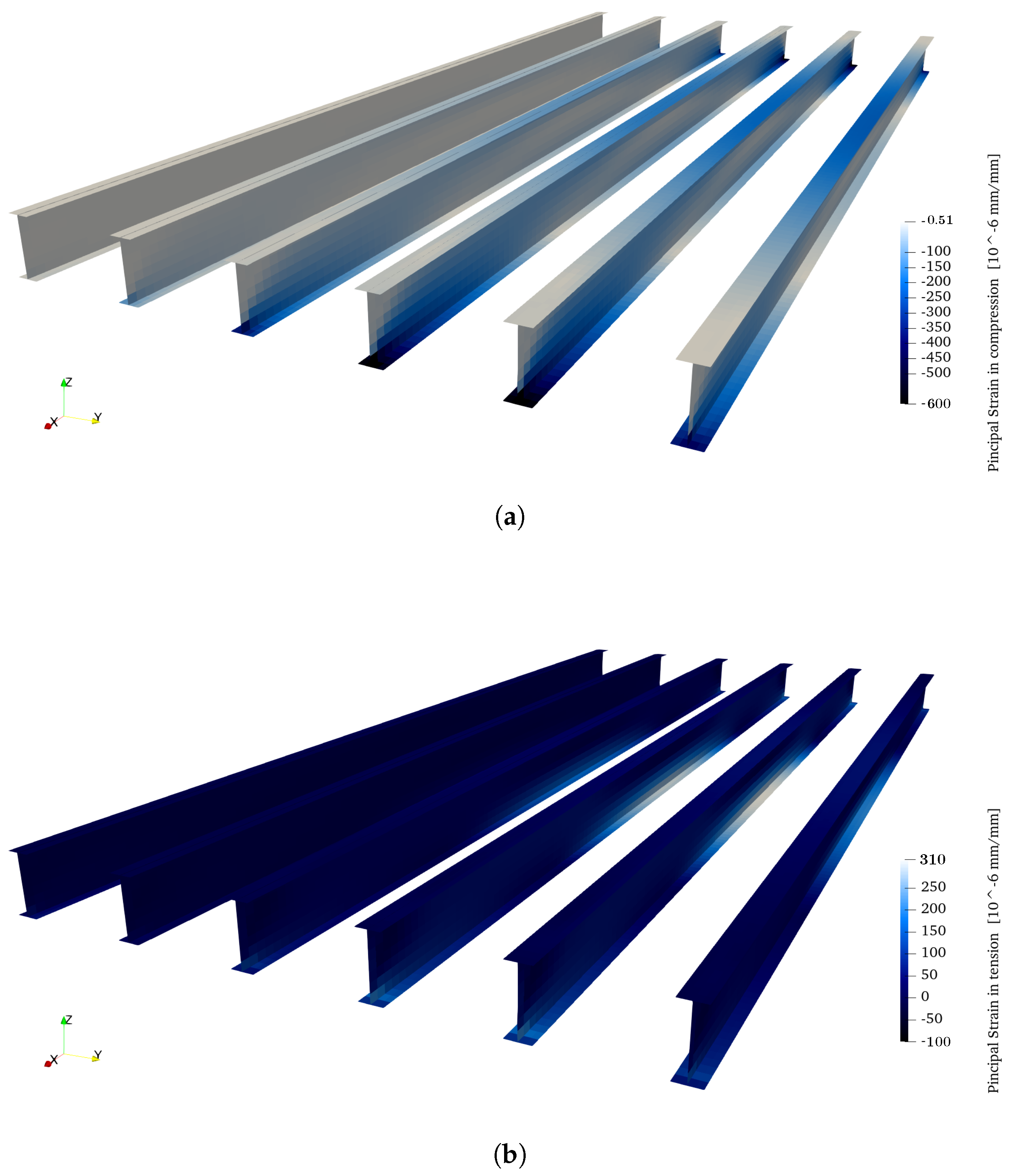
3.2. Stress Analysis

The structural analysis of the 224 bridge configurations was conducted for an $N_T$ sample of 5000 random trucks, selected based on the truck proportions listed in Table 2. The distribution of the gross weight and the axle characteristics were selected based on the parameters listed in Table 2, Table 3, and Table 4, respectively. Each span of the bridge was divided into 50 elements, and the bending and shear stresses resulting from each truck crossing were computed at each cross section of the discretized girders, as shown in the examples depicted in Figure 8. The principal stresses obtained by applying Equations (2) and (3) were analyzed as a function of different profile shapes and profile ratios. A statistical analysis of the principal stresses was conducted separately in the region of maximum positive and minimum negative bending. Figure 13 shows the average stress variation as the profile ratio of the bridges increases from 25% to 100% of the half-span length.

This reduction is on the order of 4% in both cases. The overall coefficient of variation for the stresses was found equal to be equal to 9.0%. A regression model was calibrated to describe the stress variation as a function of the profile ratio and profile shap, as shown in Equation (11), with $\rho$ expressed as a percentage. The values for the coefficients are listed in

Table 8. Stress variation regression’s parameters.

Profile Shape	Bending Type	${\mathit{a}}_0$	${\mathit{a}}_1$	Adjusted R2
P	Positive	2.64	$-5.70\times {10}^{-4}$	0.92
	Negative	2.16	$-3.89\times {10}^{-4}$	0.80
L	Positive	2.62	$-5.62\times {10}^{-4}$	0.76
	Negative	2.15	$-2.45\times {10}^{-4}$	0.79

. This equation was employed to adjust the stress ratio $S_{\sigma }$ as a function of the profile shape and $\rho$ for the reliability analysis described in the following section.

$${\sigma }_{\mathrm{avg}}=exp\left(a_0+a_1\rho \right)$$

(11)

3.3. Reliability Analysis

The reliability analysis for fatigue was conducted using the construction detail types from A to E and by adjusting the stress ratio $S_{\sigma }$ to account for the effect of the profile shape and ratio. According to a reliability-based design approach, the calibration of the safety indexes must be valid for all bridges designed within the scope of the calibrated specifications. This means that the same reliability target is chosen for all bridges. As a consequence, bridges that exhibit higher stresses are still required to meet the same reliability target. Therefore, it follows that the results presented by [40] must be valid for all $\rho$. From a constructability point of view, the fabrication of a variable girder cross section with $\rho$ smaller than 20% would be unpractical, and in that case, a girder with a constant cross section would be preferable. Hence, $\rho$ = 20% was assumed as the initial value for which the $S_{\sigma }$ parameters listed in Table 5 used by [40] are applicable to match the same safety target of the fatigue design model. Then, the random variable $S_{\sigma }$ was modified by a factor to account for the profile shape and ratio:

$$S_{\sigma ,\rho }={\displaystyle \frac{exp\left(a_0+a_1\rho \right)}{{\sigma }_{\mathrm{avg},20}}}{S}_{\sigma }$$

(12)

where ${\sigma }_{\mathrm{avg},20}$ is the average stress for a profile ratio of 20% computed with the coefficients listed in Table 8 for different profile shapes and bending type.

The reliability index for fatigue was computed with the FORM algorithm implemented into the R language for a bridge service life T equal to 75 years [79]. This is in agreement with the requirements of current bridge design specifications in the United States and Canada [73,80]. The results of the reliability analysis showed that the reliability index increases linearly with the profile ratio $\rho$. As an example, Figure 14 depicts the variation in the reliability index $\beta$ with $\rho$ for a type C construction detail, C′, which is one of the most common construction details used for I-multigirder steel bridges. This detail type includes welded joints in the transverse direction of the stress, members with sharp corners or cuts, and members with welded stiffener connections.

Figure 14 also shows that the reliability index in the region of positive bending increases from about 1.91 $\left(P_f=2.8\%\right)$ when $\rho$ = 20% to 2.01 $\left(P_f=2.2\%\right)$ when $\rho$ = 100% independently of the tapering type. In terms of the probability of failure, this change in the profile ratio corresponds to a 26.3% reduction in the probability of failure. Note that this comparison is performed relatively to each individual profile shape. However, for the same safety gain, a parabolic girder results in a lighter girder and is consequently cheaper than a girder with a variable linear profile, as shown in Figure 15. A similar scenario is depicted in Figure 14 for the negative bending region. In this case, the effect of the profile shape on $\beta$ is slightly more emphasized as the profile ratio increases. In fact, for a linear variation, the reliability index changes from 1.98 $\left(P_f=2.4\%\right)$ to 2.02 $\left(P_f=2.2\%\right)$ as $\rho$ increases, while for a parabolic girder profile, the reliability increases to 2.06 $\left(P_f=1.9\%\right)$ when $\rho$ = 100%. The analysis of results for other construction details are summarized in

Table 9. Reliability indexes.

Profile Shape	Bending Type	Detail	$\mathit{\beta }$		Reduction ${\mathit{P}}_{\mathit{f}}$ [%]
			$\mathit{\rho }$ = 20%	$\mathit{\rho }$ = 100%
Parabolic (P)	Positive	A	2.11	2.20	25.4
		B	1.80	1.90	25.1
		C, C′	1.91	2.01	26.3
		D	1.74	1.84	24.5
		E	1.76	1.86	24.7
	Negative	A	2.18	2.26	22.8
		B	1.87	1.94	17.4
		C, C′	1.98	2.06	21.1
		D	1.81	1.89	19.6
		E	1.82	1.90	19.7
Linear (L)	Positive	A	2.11	2.20	25.4
		B	1.80	1.90	25.1
		C, C′	1.91	2.00	23.4
		D	1.74	1.84	24.5
		E	1.76	1.86	24.7
	Negative	A	2.18	2.23	13.6
		B	1.87	1.91	9.5
		C, C′	1.98	2.03	12.6
		D	1.81	1.86	11.8
		E	1.82	1.87	11.8

to contain the number of figures in the manuscript. The values in the last column of Table 9 show that by increasing the profile ratio from 20% to 100%, the probability of failure in the positive bending region of continuous I-multigirder steel bridges at 75 years would reduce on the order of 25% for all construction details. In the negative region, the same probability of failure would reduce by between 10% and 14% for steel girders with a linear profile or between 17 and 23% for girders with a parabolic profile.

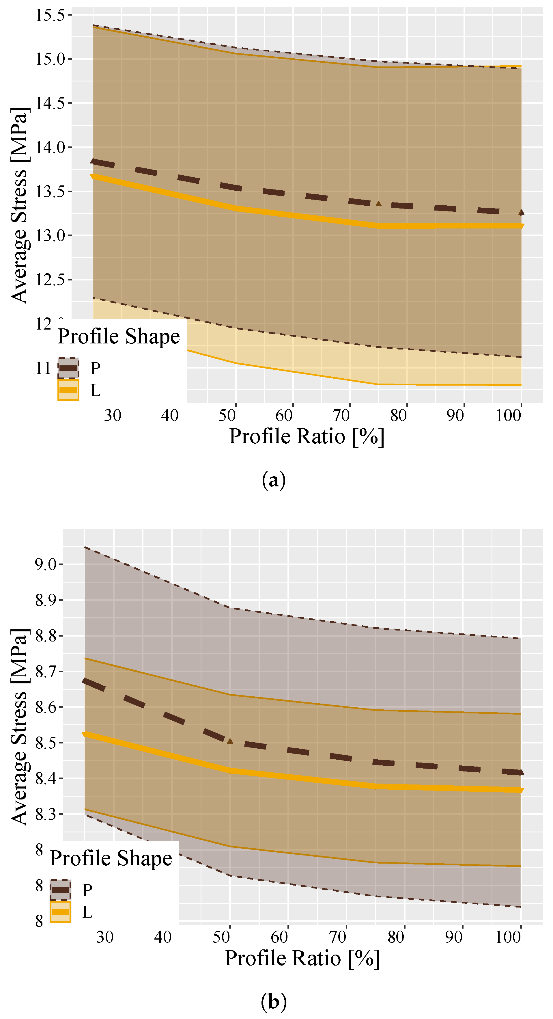
3.4. Economic Impact of Different Shape Profiles

Although for a parabolic profile, it was found to be beneficial to the reliability of bridge girders in fatigue when the profile ratio $\rho$ = 100%, it may be argued that using a curvilinear profile may add additional construction costs; this is interesting considering the costs of building different girder profiles. A relationship between the bridge weight and the stresses generated on the girders by the moving trucks was investigated as a function of the profile shape and the profile ratio $\rho$. The weight of the steel was computed for all 224 bridge configurations, and their variation with respect to the profile shape and profile ratio $\rho$ was analyzed, as depicted in Figure 15. This figure shows that the average total weight of steel of the bridge girders changes linearly with the profile ratio for both tapering types. The weights were normalized to the minimum average weight at $\rho$ = 25%. As shown in Figure 15, by imposing the same minimum and maximum cross section on the girders, the choice of linear tapering results in a slightly heavier bridge compared to a parabolic profile. In relative terms, a linear grider profile is, on average, 0.5% heavier than a parabolic profile when the profile ratio $\rho$ is equal to 25% and about 1.6% heavier when $\rho =$ 100%. In terms of the overall steel girder weight, the average total weight of the 224 bridge configurations analyzed was found to be approximately 211,000 kg considering the parabolic profile and $\rho$ equal to 25%. At the time of writing this paper, the average cost of fabricated steel plate girders, adjusted for inflation in 2024, was about 5.0 USD/kg [81]. This means that the average cost of steel for a bridge weighing 211,000 kg would be about USD 1.06M. By changing the profile ratio from 25% to 100%, the average material cost would increase by USD 26.5K and USD 43.5K for parabolic and linear profiles, respectively. This means that to build parabolic cross sections capable of reducing the fatigue probability of the failure of continuous I-girder bridges on the order of 25%, girders would have an additional material cost between 2.5% and 4.1%. This seems reasonable, given that with the advancement of manufacturing technology and the automated cutting and welding of steel, it is possible to reduce construction labour by approximately 70% [82,83]. These advanced processes will soon allow engineers to choose more optimal structural geometric shapes without incurring additional construction costs.

4. Discussion

The results presented in this paper show that different bridge configurations affect the probability of failure due to fatigue damage. A reliability analysis for fatigue was based on realistic truck traffic scenarios. In particular, in this study, data collected in Canada and the United States were analyzed. The database for the analysis was composed of data from more than 66M trucks. A statistical analysis was performed to characterize the distribution of the gross weight and axle configurations used for the numerical simulations.

A Monte Carlo simulation with 5000 realizations was performed on 224 bridge configurations, which is representative of the continuous I-multigirder steel bridge population in the United States and Canada. The structural analysis model was also validated with field measurements collected from a bridge tested to its ultimate capacity. The results of the structural analysis showed that continuous girders with a variable longitudinal profile experienced less stress as the profile ratio increases.

The results of the reliability analysis applied to the limit state function used to calibrate the AAHSTO LRFD fatigue truck showed that the probability of failure at 75 years of service in the positive bending region of continuous I-multigirder steel bridges would reduce on the order of 25% for all construction details considered in the AASHTO LRFD specifications by increasing the profile ratio from 20% to 100%, while, in the negative region, the same probability of failure would reduce by between 10% and 14% for steel girders with a linear profile and by between 17% and 23% for girders with a parabolic profile. This improvement would come with an additional material cost increase of between 2.5% and 4.1%. This increase in material cost is deemed minimum compared to the overall benefits obtained with the increased safety. It is noted that material cost is not the only cost associated with the construction of bridge girders. Complex geometries generally generate more labour time and costs. However, with the advancement of manufacturing technology and the automated cutting and welding of steel, it is possible to reduce construction labour by approximately 70%. This will soon allow engineers to choose more optimal structural geometric shapes without incurring additional construction costs. Accordingly, the results indicate that parabolic girders may become more economical than variable linear girder profiles and provide slightly increased safety given the same profile ratio.

By assessing how the longitudinal shape of these girders affects the probability of fatigue damage, government agencies and designers can better set beam geometries to minimize fatigue issues. As a consequence, the performance of steel bridges against fatigue would improve with a reduction in management costs and an increased bridge service life.

However, it should be noted that the reliability model presented in this study had some limitations. In particular, the results presented herein do not account for scenarios where random traffic patterns develop on bridge decks, which may affect the overall stress history on the girders. This is particularly important for bridges with a number of lanes greater than two and with longer span lengths, or, in numerical terms, for bridges longer than forty meters. For these cases, a microsimulation approach should be adopted.

References

1. Han, Y.; Li, K.; Cai, C.; Wang, L.; Xu, G. Fatigue reliability assessment of long-span steel-truss suspension bridges under the combined action of random traffic and wind loads. J. Bridge Eng. 2020, 25, 04020003. [Google Scholar] [CrossRef]
2. Zhou, X.; Zhang, X. Thoughts on the development of bridge technology in China. Engineering 2019, 5, 1120–1130. [Google Scholar] [CrossRef]
3. Lu, D.; Wei, W.; He, X. Optimization and application of fatigue design based on AASHTO code. China J. Highw. Transp. 2017, 30, 40. [Google Scholar]
4. Qin, S.; Gao, Z. Developments and prospects of long-span high-speed railway bridge technologies in China. Engineering 2017, 3, 787–794. [Google Scholar] [CrossRef]
5. Timoshenko, S. History of Strength of Materials: With a Brief Account of the History of Theory of Elasticity and Theory of Structures; Dover Publications: Mineola, NY, USA, 1983. [Google Scholar]
6. Fiorillo, G.; Ghosn, M. Failure Analysis of Continuous Highway Steel I-Multigirder Bridges under the Combined Effect of Fatigue and Overloading Events. J. Bridge Eng. 2025, 30, 04024105. [Google Scholar] [CrossRef]
7. Sharifi, Y. Uniform corrosion wastage effects on the load-carrying capacity of damaged steel beams. Adv. Steel Constr. 2012, 8, 153–167. [Google Scholar]
8. Schilling, C.G.; Klippstein, K.H. New method for fatigue design of bridges. J. Struct. Div. 1978, 104, 425–438. [Google Scholar] [CrossRef]
9. Schilling, C. A new method for the fatigue design of steel highway bridges. Civ. Eng. Pract. Des. Eng. 1984, 3, 541–550. [Google Scholar]
10. Agerskov, H. Fatigue in steel structures under random loading. J. Constr. Steel Res. 2000, 53, 283–305. [Google Scholar] [CrossRef]
11. Schilling, C.G. Stress cycles for fatigue design of steel bridges. J. Struct. Eng. 1984, 110, 1222–1234. [Google Scholar] [CrossRef]
12. Deng, L.; Nie, L.; Zhong, W.; Wang, W. Developing fatigue vehicle models for bridge fatigue assessment under different traffic conditions. J. Bridge Eng. 2021, 26, 04020122. [Google Scholar] [CrossRef]
13. Moses, F. Weigh-In-Motion Systems Using Instrumented Bridges. Transp. Eng. J. 1979, 105, 233–249. [Google Scholar] [CrossRef]
14. Moses, F.; Ghosn, M. Instrumentation for Weighing Trucks-In-Motion for Highway Bridge Loads, Final Report; Federal Highway Administration: Washington, DC, USA, 1983; Volume FHWA/OH-83/001. [Google Scholar]
15. Ojio, T.; Carey, C.; OBrien, E.J.; Doherty, C.; Taylor, S.E. Contactless bridge weigh-in-motion. J. Bridge Eng. 2016, 21, 04016032. [Google Scholar] [CrossRef]
16. Yan, D.; Luo, Y.; Lu, N.; Yuan, M.; Beer, M. Fatigue stress spectra and reliability evaluation of short-to medium-span bridges under stochastic and dynamic traffic loads. J. Bridge Eng. 2017, 22, 04017102. [Google Scholar] [CrossRef]
17. Alampalli, S.; Lund, R. Estimating fatigue life of bridge components using measured strains. J. Bridge Eng. 2006, 11, 725–736. [Google Scholar] [CrossRef]
18. Saberi, M.R.; Rahai, A.R.; Sanayei, M.; Vogel, R.M. Bridge fatigue service-life estimation using operational strain measurements. J. Bridge Eng. 2016, 21, 04016005. [Google Scholar] [CrossRef]
19. Kwon, K.; Frangopol, D.M.; Soliman, M. Probabilistic fatigue life estimation of steel bridges by using a bilinear S-N approach. J. Bridge Eng. 2012, 17, 58–70. [Google Scholar] [CrossRef]
20. Yen, B.T.; Hodgson, I.C.; Zhou, Y.E.; Crudele, B.B. Bilinear S-N Curves and Equivalent Stress Ranges for Fatigue Life Estimation. J. Bridge Eng. 2013, 18, 26–30. [Google Scholar] [CrossRef]
21. Leander, J.; Norlin, B.; Karoumi, R. Reliability-based calibration of fatigue safety factors for existing steel bridges. J. Bridge Eng. 2015, 20, 04014107. [Google Scholar] [CrossRef]
22. FHWA. LTBP InfoBridge; Federal Highway Administration, U.S. Department of Transportation: Washington, DC, USA, 2023. [Google Scholar]
23. CNSA. Canada’s Core Public Infrastructure Survey: Roads, Bridges and Tunnels, 2016; Canada’s National Statistics Agency: Ottawa, ON, Canada, 2016. [Google Scholar]
24. Ghosn, M.; Moses, F. Reliability calibration of bridge design code. J. Struct. Eng. 1986, 112, 745–763. [Google Scholar] [CrossRef]
25. Tabsh, S.W.; Nowak, A.S. Reliability of highway girder bridges. J. Struct. Eng. 1991, 117, 2372–2388. [Google Scholar] [CrossRef]
26. Ghosn, M.; Moses, F. Redundancy in Highway Bridge Superstructures; Number NCHRP 406; Transportation Research Board, National Cooperative Highway Research Program: Washington, DC, USA, 1998. [Google Scholar]
27. Ghosn, M. Development of Truck Weight Regulations Using Bridge Reliability Model. J. Bridge Eng. 2000, 5, 293–303. [Google Scholar] [CrossRef]
28. O’Connor, A.; O’Brien, E.J. Traffic load modelling and factors influencing the accuracy of predicted extremes. Can. J. Civ. Eng. 2005, 32, 270–278. [Google Scholar] [CrossRef]
29. Ghosn, M.; Sivakumar, B.; Miao, F. Development of State-Specific Load and Resistance Factor Rating Method. J. Bridge Eng. 2013, 18, 351–361. [Google Scholar] [CrossRef]
30. Fiorillo, G.; Ghosn, M. Procedure for statistical categorization of overweight vehicles in a WIM database. J. Transp. Eng. 2014, 140, 04014011. [Google Scholar] [CrossRef]
31. Fiorillo, G.; Ghosn, M. Fragility analysis of bridges due to overweight traffic load. Struct. Infrastruct. Eng. 2018, 14, 619–633. [Google Scholar] [CrossRef]
32. FHWA. LTPP InfoPave; Federal Highway Administration, U.S. Department of Transportation: Washington, DC, USA, 2023. [Google Scholar]
33. Nowak, A.; Hong, Y. Bridge Live Load Models. J. Struct. Eng. 1991, 121, 1245–1251. [Google Scholar] [CrossRef]
34. Fiorillo, G.; Ghosn, M. MPI Parallel Monte Carlo Framework for the Reliability Analysis of Highway Bridges. J. Comput. Civ. Eng. 2018, 32, 04017087. [Google Scholar] [CrossRef]
35. Fiorillo, G.; Ghosn, M. Risk-based importance factors for bridge networks under highway traffic loads. Struct. Infrastruct. Eng. 2018, 15, 113–126. [Google Scholar] [CrossRef]
36. Fiorillo, G.; Ghosn, M. Structural Redundancy, Robustness, and Disproportionate Collapse Analysis of Highway Bridge Superstructures. J. Struct. Eng. 2022, 148, 04022075. [Google Scholar] [CrossRef]
37. Moses, F.; Goble, G.; Pavia, A. Truck Loading Model for Bridge Fatigue. In Proceedings of the Specialty Conference on Metal Bridges American Society of Civil Engineers; American Association of State Highway and Transportation Officials, and Transportation Research Board: St. Louis, MO, USA, 1974. [Google Scholar]
38. Goble, G.; Moses, F.; Pavia, A. Applications of a bridge measurement system. Transp. Res. Rec. 1976, 579, 36–47. [Google Scholar]
39. Moses, F. Structural system reliability and optimization. Comput. Struct. 1977, 7, 283–290. [Google Scholar] [CrossRef]
40. Nyman, W.E.; Moses, F. Calibration of bridge fatigue design model. J. Struct. Eng. 1985, 111, 1251–1266. [Google Scholar] [CrossRef]
41. Yazdani, N.; Albrecht, P. Risk analysis of fatigue failure of highway steel bridges. J. Struct. Eng. 1987, 113, 483–500. [Google Scholar] [CrossRef]
42. Raju, S.K.; Moses, F.; Schilling, C.G. Reliability calibration of fatigue evaluation and design procedures. J. Struct. Eng. 1990, 116, 1356–1369. [Google Scholar] [CrossRef]
43. Laman, J.A.; Nowak, A.S. Fatigue-load models for girder bridges. J. Struct. Eng. 1996, 122, 726–733. [Google Scholar] [CrossRef]
44. Agerskov, H.; Nielsen, J.A. Fatigue in steel highway bridges under random loading. J. Struct. Eng. 1999, 125, 152–162. [Google Scholar] [CrossRef]
45. Metzger, A.T.; Huckelbridge, A.A., Jr. Temporal nature of fatigue damage in highway bridges. J. Bridge Eng. 2009, 14, 444–451. [Google Scholar] [CrossRef]
46. Wang, C.S.; Hao, L.; Fu, B.N. Fatigue reliability updating evaluation of existing steel bridges. J. Bridge Eng. 2012, 17, 955–965. [Google Scholar] [CrossRef]
47. Zhang, W.; Cai, C. Fatigue reliability assessment for existing bridges considering vehicle speed and road surface conditions. J. Bridge Eng. 2012, 17, 443–453. [Google Scholar] [CrossRef]
48. Bowman, M.D.; Fu, G.; Zhou, Y.E.; Connor, R.J.; Godbole, A.A. Fatigue Evaluation of Steel Bridges; Volume NCHRP Report 721; Transportation Research Board, National Academy Press: Washington, DC, USA, 2012. [Google Scholar]
49. Putri, C.A.; Tateishi, K.; Shimizu, M.; Hanji, T. Failure probability for fatigue crack in web plate of bridge girder. Int. J. Steel Struct. 2022, 22, 42–55. [Google Scholar] [CrossRef]
50. Croce, P. Background to fatigue load models for Eurocode 1: Part 2 Traffic Loads. Prog. Struct. Eng. Mater. 2001, 3, 335–345. [Google Scholar] [CrossRef]
51. Zhou, Y.; Zhai, H.; Bao, W.; Liu, Y. Research on standard fatigue vehicular load for highway bridges. Highway 2009, 12, 21–25. [Google Scholar]
52. Chen, W.z.; Xu, J.; Yan, B.c.; Wang, Z.p. Fatigue load model for highway bridges in heavily loaded areas of China. Adv. Steel Constr. 2015, 11, 322–333. [Google Scholar]
53. Liu, Y.; Li, D.; Zhang, Z.; Zhang, H.; Jiang, N. Fatigue load model using the weigh-in-motion system for highway bridges in China. J. Bridge Eng. 2017, 22, 04017011. [Google Scholar] [CrossRef]
54. Han, X.; Frangopol, D.M. Fatigue reliability analysis considering corrosion effects and integrating SHM information. Eng. Struct. 2022, 272, 114967. [Google Scholar] [CrossRef]
55. Fisher, J.W.; Frank, K.H.; Hirt, M.A.; McNamee, B.M. Effect of Weldments on the Fatigue Strength of Steel Beams; Number NCHRP Report 102; Transportation Research Board, National Cooperative Highway Research Program: Washington, DC, USA, 1970. [Google Scholar]
56. Fisher, J.W.; Mertz, D.R.; Zhong, A. Steel Bridge Members Under Variable Amplitude Long Life Fatigue Loading; Number NCHRP Report 267; Transportation Research Board, National Cooperative Highway Research Program: Washington, DC, USA, 1983. [Google Scholar]
57. Dexter, R.J.; Wright, W.J.; Fisher, J.W. Fatigue and fracture of steel girders. J. Bridge Eng. 2004, 9, 278–286. [Google Scholar] [CrossRef]
58. Miner, M.A. Cumulative damage in fatigue. J. Appl. Mech. 1945, 12, 149–164. [Google Scholar] [CrossRef]
59. McConnell, J.R.; Almoosi, Y.S. Field Evaluation of Fatigue Stresses in a Modern Highly Skewed Steel I-Girder Bridge. J. Bridge Eng. 2022, 27, 04022005. [Google Scholar] [CrossRef]
60. Sivakumar, B.; Ghosn, M.; Moses, F. Protocols for Collecting and Using Traffic Data in Bridge Design; Number NCHRP Report 683; Transportation Research Board, National Academy Press: Washington, DC, USA, 2011. [Google Scholar]
61. Chotickai, P.; Bowman, M.D. Truck models for improved fatigue life predictions of steel bridges. J. Bridge Eng. 2006, 11, 71–80. [Google Scholar] [CrossRef]
62. Grubb, M.A.; Wilson, K.E.; White, C.D.; Nickas, W.N. Load and Resistance Factor Design (LRFD) for Highway Bridge Superstructures-Reference Manual; Technical Report; Federal Highway Administration, U.S. Department of Transportation: Washington, DC, USA, 2015. [Google Scholar]
63. Ghosn, M.; Yang, J.; Beal, D.; Sivakumar, B. Bridge System Safety and Redundancy; Number NCHRP Report 776; Transportation Research Board, National Academy Press: Washington, DC, USA, 2014. [Google Scholar]
64. Ghosn, M.; Fiorillo, G.; Gayovyy, V.; Getso, T.; Ahmed, S.; Parker, N. Effect of Overweight Vehicles on NYSDOT Infrastructure; Number NYSDOT C-08-13; New York State Department of Transportation: Albany, NY, USA, 2015. [Google Scholar]
65. Pushka, A.; Regehr, J.D.; Fiorillo, G.; Mufti, A.; Algohi, B. Reliability analysis of typical highway bridges in Manitoba designed to the Modified HSS-25 live load model. Can. J. Civ. Eng. 2022, 49, 899–909. [Google Scholar] [CrossRef]
66. USDOT. Traffic Monitoring Guide; Federal Highway Administration: Washington, DC, USA, 2022. [Google Scholar]
67. Fiorillo, G. Reliability and Risk Analysis of Bridge Networks. Ph.D. Thesis, The City College of the City University of New York (CUNY), New York, NY, USA, 2016. [Google Scholar]
68. Gere, J.M.; Timoshenko, S.P. Mechanics of Materials; International Thomson Publishing: Boston, MA, USA, 1990. [Google Scholar]
69. McKenna, F.; Scott, M.H.; Fenves, G.L. Nonlinear Finite-Element Analysis Software Architecture Using Object Composition. J. Comput. Civ. Eng. 2010, 24, 95–107. [Google Scholar] [CrossRef]
70. Ramberg, W.; Osgood, W. Description of Stress Strain Curves by Three Parameters; Techincal Note No. 902; National Advisory Committee for Aeronautics: Washington, DC, USA, 1943. [Google Scholar]
71. Gaylord, E.H.; Gaylord, C.N. Structural Engineering Handbook; McGraw-Hill: New York, NY, USA, 1990. [Google Scholar]
72. Courbon, J. Design of Multi-Beam Bridges with Intermediate Diaphragms (Calcul des Ponts a Poutres Multiples Solidarisees par des Entretoises). Ann. Des Ponts 1940, 17, 115–116. [Google Scholar]
73. AASHTO. AASHTO LRFD Bridge Design Specifications, 9th ed.; American Association of State Highway and Transportation Officials, Inc.: Washington, DC, USA, 2020. [Google Scholar]
74. Caprani, C.C. Calibration of a congestion load model for highway bridges using traffic microsimulation. Struct. Eng. Int. 2012, 22, 342–348. [Google Scholar] [CrossRef]
75. Schijve, J. A normal distribution or a Weibull distribution for fatigue lives. Fatigue Fract. Eng. Mater. Struct. 1993, 16, 851–859. [Google Scholar] [CrossRef]
76. Rackwitz, R.; Flessler, B. Structural reliability under combined random load sequences. Comput. Struct. 1978, 9, 489–494. [Google Scholar] [CrossRef]
77. Bakht, B.; Jaeger, L.G. Ultimate load test of slab-on-girder bridge. J. Struct. Eng. 1992, 118, 1608–1624. [Google Scholar] [CrossRef]
78. EDF. Electricité de France, Finite Element Code_Aster, Analysis of Structures and Thermomechanics for Studies and Research. 2024. Available online: www.code-aster.org (accessed on 1 February 2025).
79. R Core Team. R: A Language and Environment for Statistical Computing; R Foundation for Statistical Computing: Vienna, Austria, 2024. [Google Scholar]
80. CSA S6:19; Canadian Highway Bridge Design Code. Canadian Standard Association: Toronto, ON, Canada, 2019.
81. RSMeans. Heavy Construction Cost Data; R.S. Means Co.: Kingston, MA, USA, 2009. [Google Scholar]
82. Irco, A. Bridge Girder Manufacturing. 2025. Available online: https://ircoautomation.com/bridge-girder-manufacturing/ (accessed on 25 March 2025).
83. Sarivan, I.M.; Madsen, O.; Wæhrens, B.V. Automatic welding-robot programming based on product-process-resource models. Int. J. Adv. Manuf. Technol. 2024, 132, 1931–1950. [Google Scholar] [CrossRef]
Figure 1. Continuous steel bridges with a variable profile. (a) Linear (L) variation. (b) Parabolic (P) variation.
Infrastructures 10 00092 g001
Figure 2. Continuous steel girder with a small profile ratio ρ .
Infrastructures 10 00092 g002
Figure 3. Variable girder cross section profile. (a) Linear (L) variation. (b) Parabolic (P) variation.
Infrastructures 10 00092 g003
Figure 4. WIM station locations.
Infrastructures 10 00092 g004
Figure 5. Gross vehicle weight histograms. (a) Class 5, (b) Class 6, (c) Class 8, (d) Class 9, (e) Class 10, and (f) Class 13.
Infrastructures 10 00092 g005
Figure 6. Fatigue analysis of a continuous I-multigirder steel composite bridge. (a) Tridimensional view. (b) Girder profiles and stress tensors as a function of the truck position.
Infrastructures 10 00092 g006
Figure 7. Bridge finite element model in OpenBRAIN.
Infrastructures 10 00092 g007
Figure 8. Bridge response to 10 random trucks. (a) Moment response at section x = 10 m. (b) Moment response at section x = 19.5 m. (c) Shear response at section x = 10 m. (d) Shear response at section x = 19.5 m.
Infrastructures 10 00092 g008
Figure 9. Transverse truck load position. (a) Single truck. (b) Side-by-side events.
Infrastructures 10 00092 g009
Figure 10. Annual Daily Truck Traffic distribution from the LTPP WIM sites in 2012.
Infrastructures 10 00092 g010
Figure 11. Typical fatigue details of highway steel bridges according to [73]. (a) Type B, built of plates and shapes connected by a continuous longitudinal complete penetration weld. (b) Type B or C, welded joints in the transverse direction of the stress. (c) Type C, members with re-entrant corners or cuts. (d) Type C′, members with welded stiffener connections.
Infrastructures 10 00092 g011
Figure 12. FEM model of the Stoney Creek bridge. (a) Strain in compression. (b) Strain in tension.
Infrastructures 10 00092 g012
Figure 13. Stress vs. profile ratio. (a) Positive bending. (b) Negative bending.
Infrastructures 10 00092 g013
Figure 14. Reliability index vs. profile ratio for construction detail C, C′. (a) Positive bending. (b) Negative bending.
Infrastructures 10 00092 g014
Figure 15. Steel girders weight change as a function of profile shape and profile ratio ρ .
Infrastructures 10 00092 g015