Point Transformer Network-Based Surrogate Model for Spatial Prediction in Bridges

Abstract

Bridges are essential assets of inland transportation infrastructure; however, they are among the most vulnerable elements of these networks due to deterioration caused by aging and the increasing loads to which they are subjected over time. Consequently, maintenance becomes critical to ensure acceptable levels of safety and service. Finite element (FE) models are traditionally used to reliably assess structural health, but their computational expense often prevents their extensive use in routine bridge assessments. To overcome this computational limitation, this paper presents an innovative deep learning-based surrogate model for predicting local displacements in bridge structures. By utilizing point cloud data and transformer neural networks, the model provides fast and accurate predictions of displacements, addressing the limitations of traditional methods. A case study of a historical bridge demonstrates the model’s efficiency. The proposed approach integrates spatial data processing techniques, offering a computationally efficient alternative for bridge health monitoring. Our results show that the model achieves mean absolute errors below 0.0213 mm, drastically reducing the time required for structural analysis.

1. Introduction

Bridges serve as critical arteries in the global transportation network, underpinning economic growth, enabling social integration, and facilitating efficient movement across geographic obstacles. In 2023, there were a total of 621,581 highway bridges in the United States [1]. Despite their importance, aging bridge infrastructure presents a formidable challenge, threatening not only economic vitality but also public safety. In fact, it has been reported that 42% of the bridges in the United States are more than 50 years old, and 7.5% are now classified as structurally deficient [2], highlighting an urgent need for comprehensive maintenance and monitoring strategies to avoid potential failures that could have catastrophic consequences.

The degradation of infrastructure can result from different types of factors, both natural, such as earthquakes, floods, and corrosion due to environmental conditions, and anthropogenic, including overloading and lack of timely maintenance [3,4], among others. These challenges highlight the need for innovative approaches to infrastructure management and maintenance.

In recent decades, many cost-effective Structural Health Monitoring (SHM) technologies have emerged, including advancements in non-destructive testing, the Internet of Things (IoT), and advanced sensor networks. These innovations represent a crucial transition from conventional inspection techniques toward next-generation monitoring technologies, enabling accurate, real-time evaluations of the structural health of bridges throughout their aging process [5,6,7,8]. However, despite these technological advances, significant room for innovation remains—especially at the intersection of SHM and new computational approaches that ensure the accuracy of numerical models such as finite element (FE) models.

Within finite element modelling, different approaches or levels of simplification can be used (e.g., solids, shells, and beams). Solid models offer the highest accuracy but incur a substantial computational cost. In contrast, beam models, which involve a high degree of simplification, impose the lowest computational burden. Shell models provide a middle ground, balancing computational load and accuracy. Nevertheless, when analyzing large structures or performing numerous simulations, the computational cost becomes a barrier that reduces practicality and can even be prohibitive.

In response to this barrier, the field of artificial intelligence (AI) has experienced remarkable growth, with deep learning emerging as a foundational element of current research. Deep learning algorithms, renowned for their ability to autonomously learn from data, have led to significant progress in areas such as computer vision and natural language processing. This progress is supported by the widespread availability of large datasets and rapidly expanding computational power, enabling the development of sophisticated models that interpret the world with unprecedented precision.

In response to this development, Artificial Neural Networks (ANNs) have been suggested as a more efficient and accurate alternative to FE models [9]. In fact, different architectures of ANN such as Multi-Layer Perceptron (MLP) and Long Short-Term Memory (LSTM) networks have been proposed to create surrogate models of bridges [10,11,12,13]. Moreover, applying deep learning to spatial data processing has opened new avenues for innovation. By adeptly handling the complexities of spatial structures and relationships, deep learning technologies have enabled advancements ranging from enhancing autonomous vehicle systems to optimizing urban planning and infrastructure management [14,15,16,17,18,19,20]. These applications underscore the transformative impact of deep learning, ushering in a new era of data analysis that is both more precise and adaptable to the intricate realities of our physical environment.

Among the various types of spatial data processed by deep learning algorithms, 3D point clouds represent a critical category. These point clouds consist of points in three-dimensional space that accurately capture the external surfaces of objects. Their application—primarily in classification, segmentation, and detection tasks—has shown significant promise [14,21,22,23,24]. Researchers have explored diverse methodological approaches to effectively utilize point cloud data’s inherent information.

Regarding deep learning’s potential for regression tasks within point clouds, this task remains largely unexplored. However, some applications show promising results. For example, in environmental remote sensing, the authors from [25] regressed above-ground biomass and carbon stocks from airborne LiDAR without relying on a terrain model, thereby enabling large-scale forest carbon mapping. Similarly, in [26], the authors developed a Biomass Prediction Network (BioNet) to predict crop plot biomass from LiDAR scans. Their approach outperformed traditional methods by approximately 33% in accuracy. In robotics and autonomous systems, 3D point clouds from LiDAR are used for regressing bounding box coordinates for 3D object detection [27,28] or estimating a robot’s pose from raw 3D data [29], demonstrating that deep networks can successfully map unstructured point clouds to continuous outputs required for navigation and mapping.

Moreover, emerging research in 3D spatial simulation and geometry processing shows that point cloud networks can serve as fast surrogates for complex physics simulations. For instance, in [30], authors employed a PointNet-based model to map spatial coordinates of an airflow domain directly to flow quantities, predicting the fluid flow field around objects. Their network preserved fine geometric detail without the need to rasterize the input to a grid and achieved predictions hundreds of times faster than conventional computational fluid dynamics (CFD) solvers. These examples highlight the applicability of point cloud regression.

Although traditional deep learning approaches have been employed to create surrogate models, specific architectures tailored for spatial data processing have not yet been applied to this task, to the best of our knowledge. In light of this, we have conducted a study that addresses this gap by applying point cloud deep learning techniques for point-wise regression, aiming to precisely calculate the spatial attributes of object surfaces. This method not only broadens the scope of deep learning in spatial data analysis but also introduces an innovative approach to infrastructure monitoring—particularly focusing on the health of bridges.

The remaining sections of the paper are structured as follows. Section 2 explains the proposed methodology used to obtain surrogate models of bridges using deep learning, Section 3 presents the case study and how the methodology has been applied, Section 4 presents the results obtained in the case study and discusses the results. Finally, in Section 5, the conclusions are presented.

2. Methodology

This section presents the methodology developed to create a surrogate model using deep learning. To demonstrate its effectiveness, the proposed approach is applied to a historical bridge.

The primary objective of the method is to predict local displacements of bridge surfaces under varying load conditions. To achieve this, the model incorporates several critical inputs: the geometry of the bridge (represented as a 3D point cloud), and the point and distributed loads defined by load model 71 of the Eurocode [31]. The primary objective of the method is to predict local displacements of bridge surfaces under varying load conditions. To achieve this, the model incorporates several critical inputs: the geometry of the bridge (represented as a 3D point cloud), and the point and distributed loads defined by load model 71 of the Eurocode.

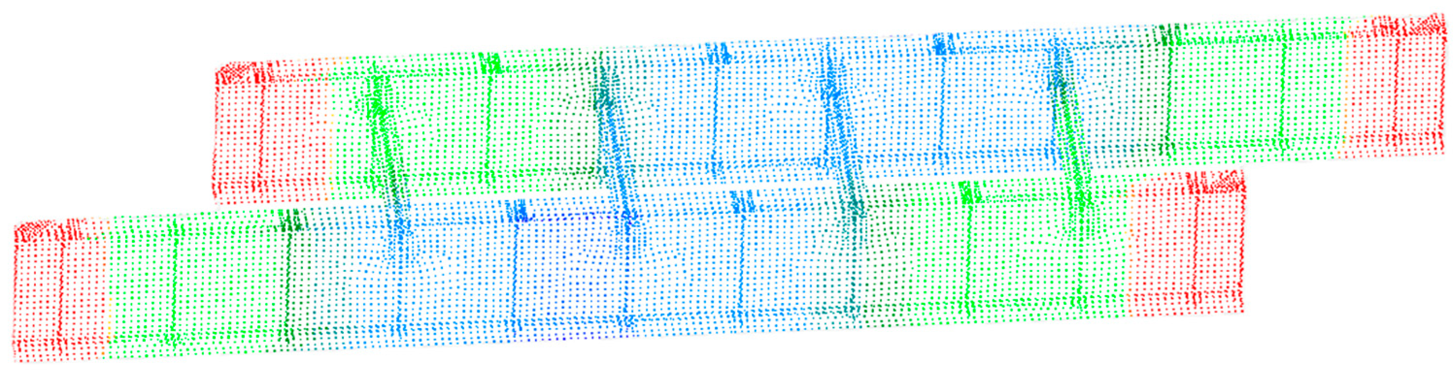
The geometry of the bridge is represented as a 3D point cloud—a set of discrete points defined in a three-dimensional coordinate system that correspond to the surfaces of the objects present in the scanned environment (in this case, the bridge structure). Depending on the acquisition technology, additional attributes such as color, reflectivity, and other surface features may also be included.

For this study, point clouds of the bridge were obtained with varying levels of precision, allowing us to assess the influence of geometric accuracy on the model’s performance. An example of the bridge point cloud is shown in Figure 1.

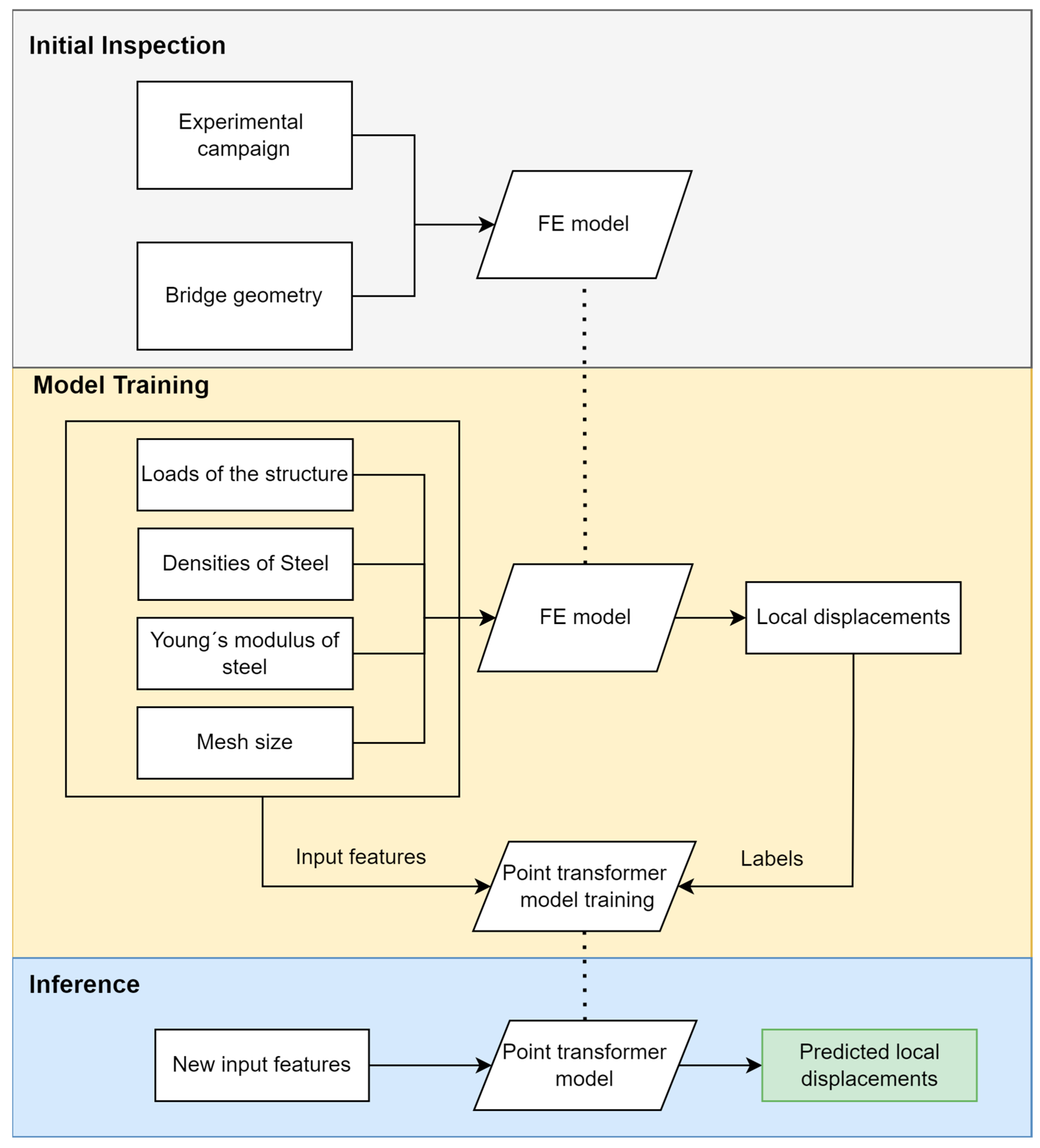
The proposed methodology is summarized in Figure 2. It begins with an initial inspection during which the data required to build the FE model is gathered. Next, the data generated by the FE model—providing high-fidelity displacement results under various loading conditions—serve as the ground truth for training a neural network. Once trained, the neural network uses the spatial features of the bridge geometry and the loading conditions as inputs to predict local displacements across the entire structure, offering a computationally efficient alternative to traditional FE model analysis.

2.1. Deep Learning Model

As highlighted in the introduction, the application of deep learning to point cloud data has been growing in recent years. This growth has primarily focused on classification, segmentation, and registration tasks. However, in this work, we propose to employ 3D deep learning neural networks for regression, providing point-wise local displacements along the three coordinate axes and thereby expanding the scope of deep learning applications on point cloud data.

Regarding deep learning architectures, transformers have emerged as a groundbreaking innovation—particularly in sequence-to-sequence tasks in Natural Language Processing (NLP). Introduced in [32], transformers bypass the sequential processing of earlier models like RNNs and LSTMs by processing data in parallel. Their core innovation, the attention mechanism, allows the model to weigh the significance of different parts of the input data, enabling it to focus on the most relevant information without being constrained by order. The success of transformers in NLP is largely due to their ability to handle long-range dependencies and contextual nuances. Leveraging vast datasets and extensive computational power, transformers learn patterns and relationships with unprecedented precision.

Building on this success, researchers have adapted transformer architectures for processing point clouds [33,34,35,36]. Point clouds are inherently unordered and structurally distinct from text, posing unique analytical challenges. With their attention mechanisms, transformers provide a novel solution by treating each point as a “word” in a “sentence”, thereby learning complex spatial relationships and features. This represents a significant shift from conventional point cloud processing techniques, which often rely on hand-crafted features or convolutions that may not fully capture spatial relationships.

Based on the above, the deep learning model proposed for this task is built on transformer architectures, specifically leveraging the segmentation model “Point Transformer” as introduced in [24].

2.2. Model Architecture

The original architecture of the Point Transformer consists of several layers specifically designed for point clouds, utilizing vector self-attention mechanisms. This design enables the network to effectively process spatial data embedded in 3D space by treating it as a set of unordered points. The network’s backbone is structured to efficiently handle large datasets while maintaining scalability. The layers constituting the model are as follows:

Point Transformer layer: This layer applies vector self-attention locally within neighborhoods defined by the k nearest neighbors of each point. The self-attention mechanism in the Point Transformer inherently learns relationships between points, capturing both local and global spatial dependencies. This helps ensure that predicted displacements remain smooth across adjacent points, preventing abrupt variations.

Position encoding: The use of trainable position encodings enhances the network’s ability to incorporate spatial relationships into the model, providing it with the capability to better interpret complex spatial structures. This relative spatial information reinforces the continuity of displacements across the structure.

Residual Point Transformer blocks: These blocks incorporate self-attention layers with linear transformations, enhancing the network’s depth and enabling more complex and abstract representation learning.

To adapt the Point Transformer for regression tasks, the primary modification involves the replacement of the network’s last layer. The last segmentation layer is replaced with a fully connected linear layer that maps the high-dimensional features learned by the transformer layers to 3 scalar values per point, which will provide the predicted displacements of the given point.

To accommodate regression, changes in the loss function are required. In this case, the loss is replaced by Mean Squared Error (MSE), focusing on minimizing the prediction error. Since adjacent points in the point cloud often have similar displacement values, minimizing MSE inherently encourages smooth transitions between adjacent points.

Finally, regarding the parameters chosen to build the architecture, they are based on the implementation described in the original Point Transformer paper [24]. The number of encoder layers that the original work has was used. However, different configurations for the number of attention heads and the number of nearest neighbors (k) were tested. The experiments demonstrated that using 4 attention heads provided the best results for the given dataset. Furthermore, several combinations of k-values were tested, but the results showed that the optimal configuration is the one from the original implementation, using 8 neighbors in the first encoder layer and 16 in subsequent stages. Also, it is important to note that, since the dataset exhibits variable point densities depending on the mesh size used for each simulation, the optimal k may vary locally. The other parameters used to define the architecture, and a short description are shown in

Table 1. Parameters and descriptions of the Point Transformer architecture.

Parameter	Values	Description
Encoder Layers	[2, 3, 4, 6, 3]	Number of transformer blocks at each stage of the encoder.
Channels	[32, 64, 128, 256, 512]	Number of output channels for each encoder stage.
k-Nearest Neighbors	[8, 16, 16, 16, 16]	Number of nearest neighbors used at each stage.
Strides	[1, 4, 4, 4, 4]	Downsampling factor at each encoder stage.
Attention Heads	4	Number of attention heads.

.

3. Case Study

3.1. Description of the Bridge and Experimental Campaign

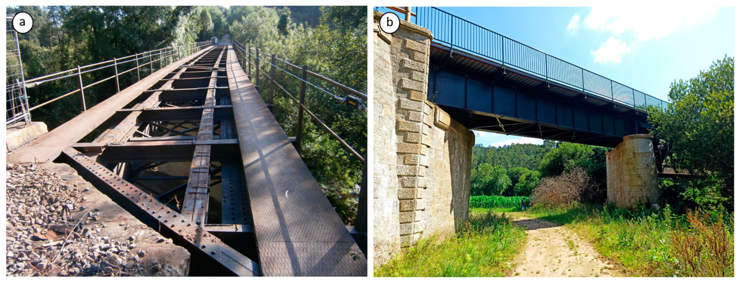
For the implementation of the proposed methodology, a steel railway bridge located in Vilagarcía de Arousa—a region in the west of Galicia, Spain—was selected as a case study and it is shown in Figure 3. Constructed in 1897 by the English firm Joseph Westwood & Co., London, the Unitied Kingdom, the bridge was part of the railway line connecting Pontevedra and Vilagarcía de Arousa and remained operational until 2008. In 2020, it was renovated and later repurposed for pedestrian use. The structure, made of riveted steel, spans 15.6 m in length and 5.8 m in width and is supported by two masonry abutments. All steel components are fabricated from riveted steel plates and L-shaped profiles. The bridge’s structural composition includes two principal girders (each 1.57 m in height with flanges 0.38 m wide) interconnected by four cross-girders. Lateral reinforcement of the main girders is provided by twenty-six web stiffeners and thirty-one L-shaped bracings, while a frame consisting of two longitudinal and seven transverse beams rests atop the main and cross-girders to facilitate load distribution.

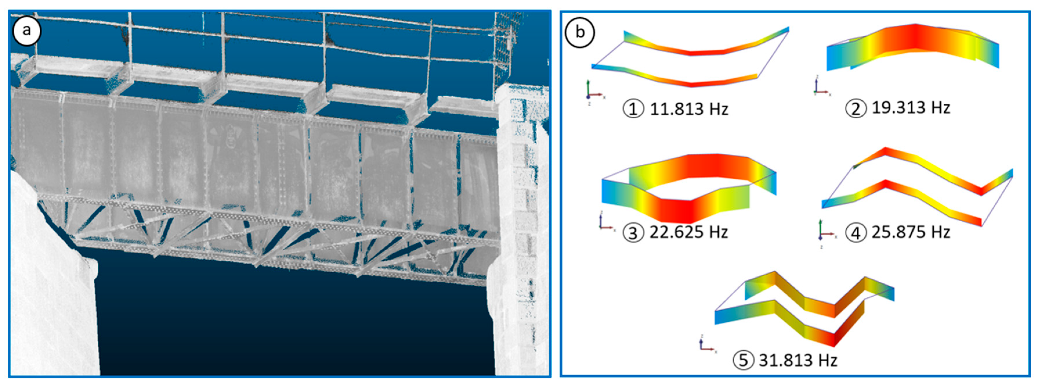
The characterization and FE modelling of the bridge were carried out in a preliminary study in which an algorithm for damage prediction was developed [37]. The experimental campaign involved several steps. First, a visual inspection and in situ measurements were conducted using a digital gauge for geometrical characterization. This was complemented by a terrestrial laser scanner survey. Finally, the dynamic behavior of the bridge was assessed using an Ambient Vibration Test (AVT), which yielded five vibration modes subsequently used to calibrate the FE model. Figure 4 illustrates the obtained point cloud and the AVT results; further details on the experimental development can be found in [37].

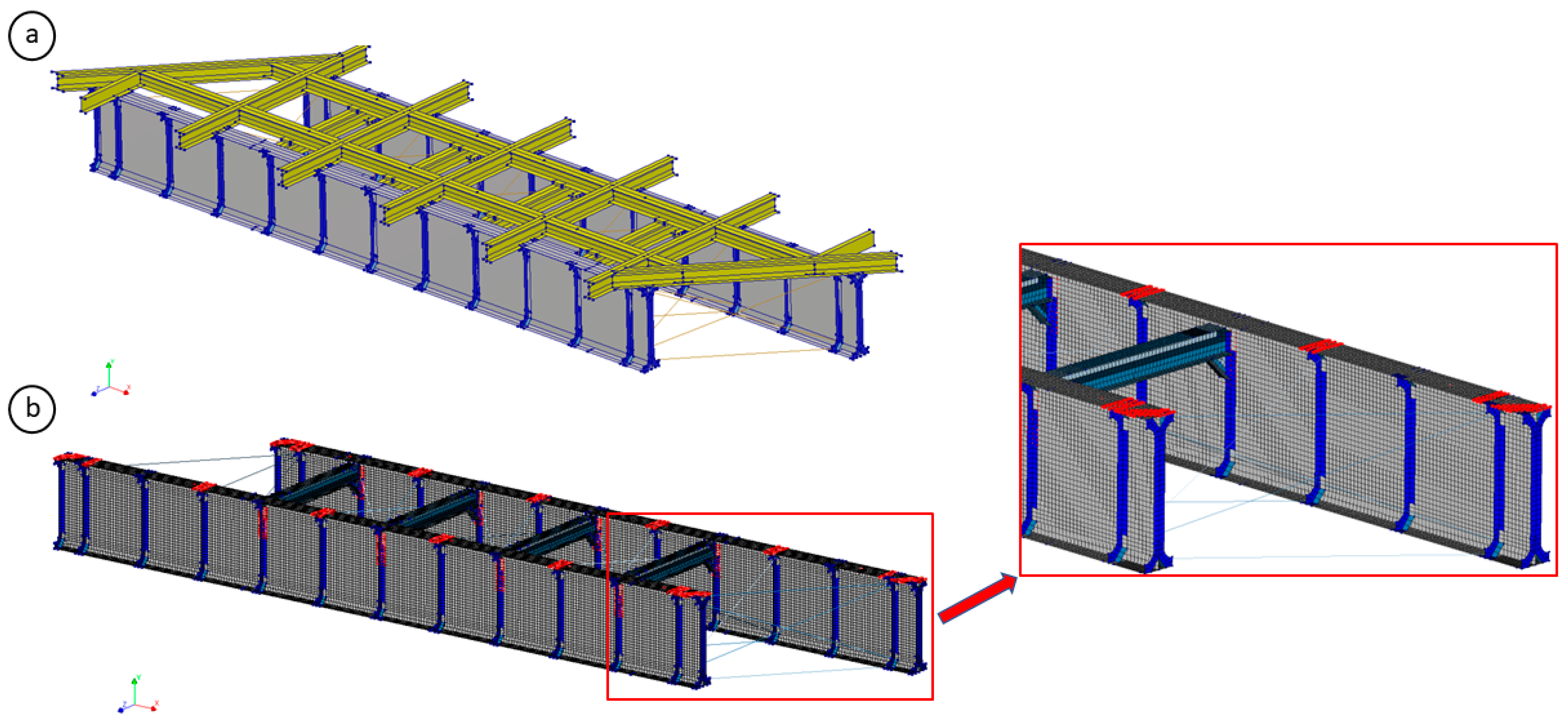
3.2. FE Modelling and Updating

Once the structure was properly characterized, the FE modelling was performed using the software Diana FEA 10.10 [38]. Four-node quadrilateral isoparametric shell elements were used for all bridge components, except for the bracings, which were modeled using two-node truss elements. This shell modelling approach renders the case study challenging due to the large number of Degrees of Freedom (DoFs) generated in the mesh, which depends on the chosen element size. For example, assuming a mesh size of 0.05 m, 31,545 nodes are generated, resulting in a total of 94,635 DoFs. Prior to calibration, the upper frame was replaced with an equivalent mass because its connection did not contribute stiffness and its sole function was to redistribute loads. The reliability of this approach was corroborated by comparing structural responses with AVT results, where errors were substantially reduced. Figure 5 shows both the original FE model and the pre-calibration model (with a 0.05 m mesh size).

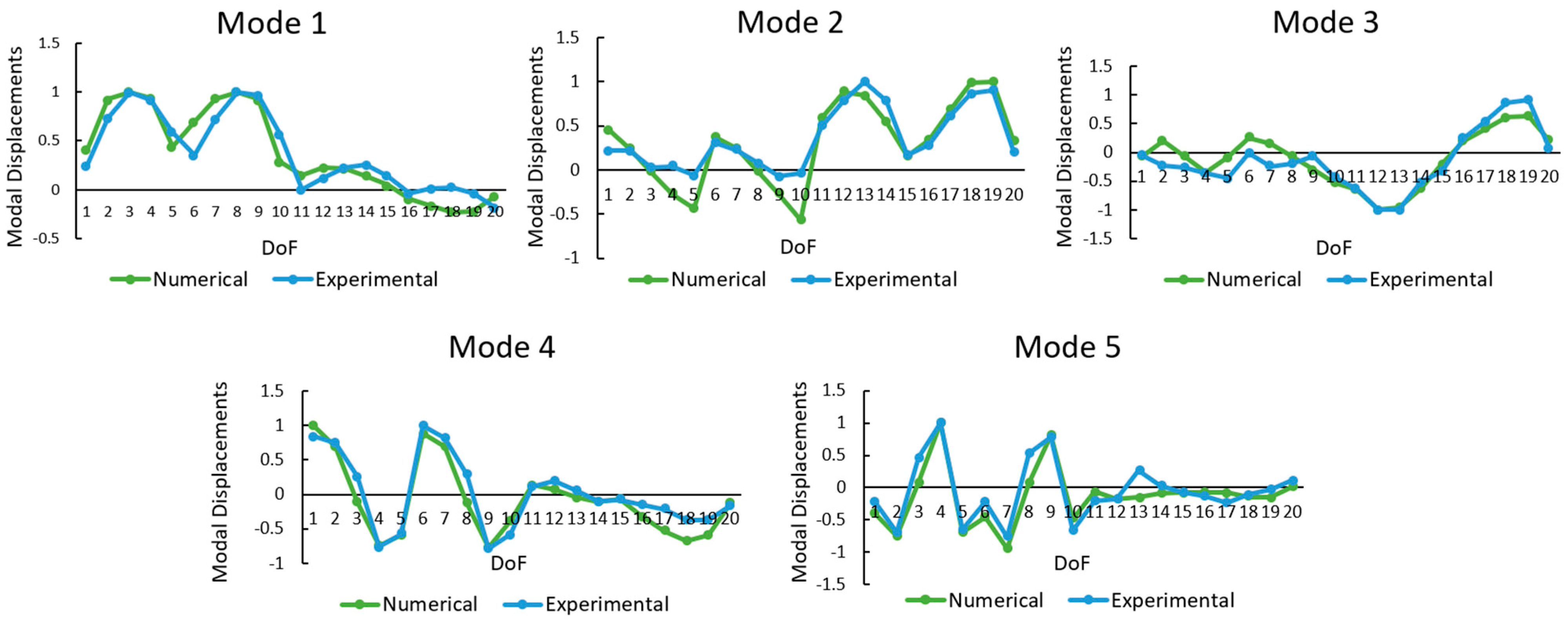
The calibration process was then carried out to ensure that the FE model accurately represented the real structure. Details of the calibration are discussed in [37]. The variables considered during calibration included the steel properties (density and Young’s modulus), the corroded thickness of various elements, and the stiffness of the interfaces representing the soil–structure interaction and the support. Discrepancies between the FE model and the real structure were measured in terms of frequencies and modal displacements. A gradient-based method (lsqnonlin from the MATLAB 9.13.0 (R2022b) optimization toolbox) was employed to minimize these discrepancies [39]. As a result, the differences between the FE model and the experimental response (as measured in the AVT) were minimized. Figure 6 shows a graphical comparison of the modal displacements, and

Table 2. Comparison between the experimental (AVT) and numerical (FE model) frequencies.

Mode	Experimental Frequency (AVT)	Numerical Frequency (FE Model)	Relative Error (%)
1	11.81 Hz	11.90 Hz	0.76%
2	19.31 Hz	19.36 Hz	0.26%
3	22.63 Hz	22.64 Hz	0.04%
4	25.88 Hz	25.91 Hz	0.12%
5	31.81 Hz	31.84 Hz	0.09%

summarizes the frequencies and their corresponding errors, demonstrating that the numerical model represents the bridge’s dynamic behavior with high accuracy.

3.3. Dataset Generation

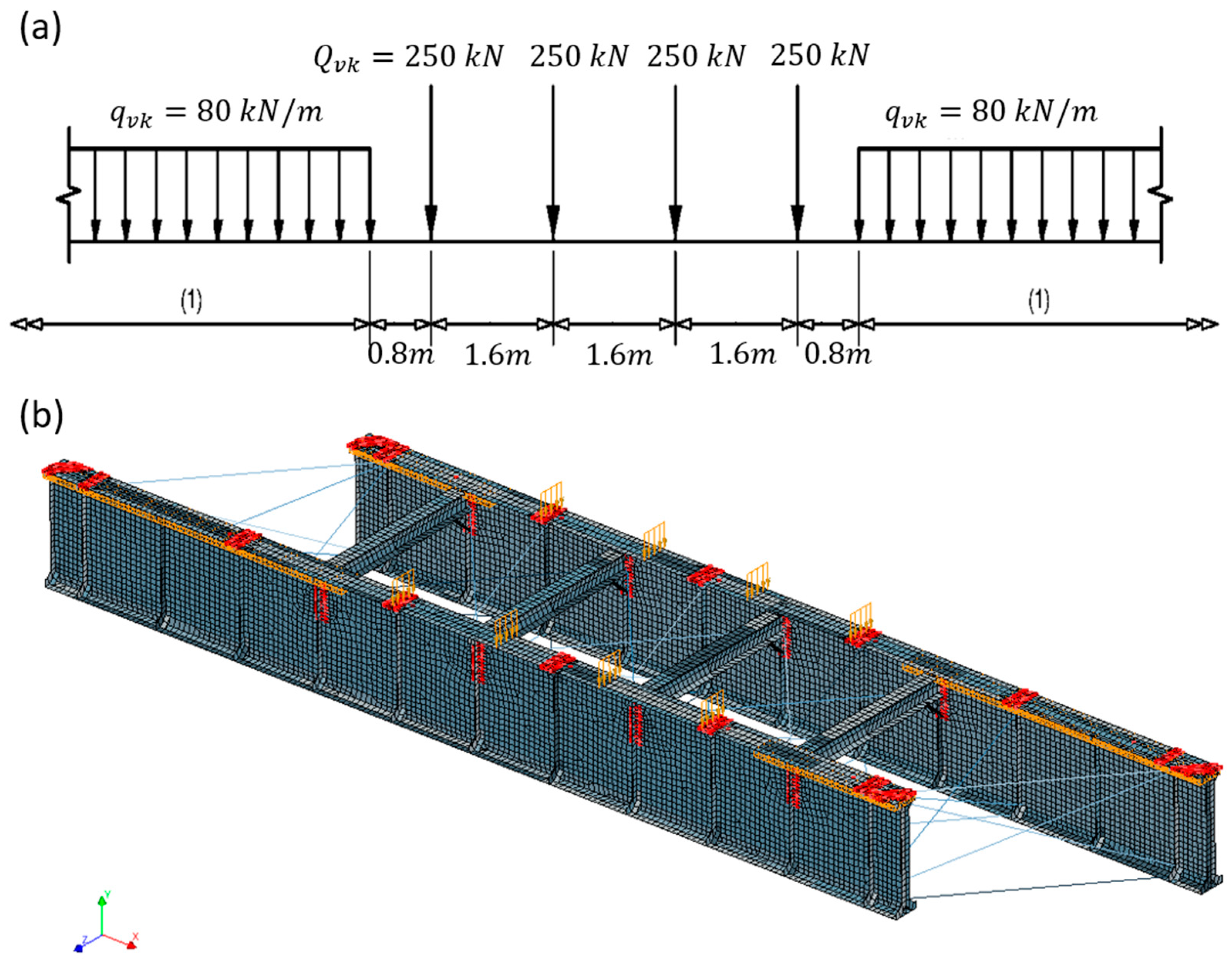
Once the modelling process was completed, the dataset for the training of the deep learning-based surrogate model proposed in the methodology was created. As variables of the model and therefore of the surrogate model, the following were considered: (i) the loads of the structure, (ii) density of steel, (iii) Young’s modulus of steel, and (iv) the mesh size of the FE model. For the load modelling, considering the purpose for which the bridge was designed (railway), it was chosen to use the load model 71 of the Eurocode that represents normal railway traffic on main lines [31]. The characteristic load magnitudes are defined at the 98th percentile of a Gumbel probability distribution for a 50-year return period, yielding mean values of 207.4 kN for the point load and 63.4 kN/m for the distributed load. Using a Coefficient of Variation (CoV) of 10% [40,41,42] and considering the area over which the load is applied, equivalent distributions were computed. Figure 7 illustrates load model 71 and the load application areas (highlighted in orange).

Regarding the material properties, the density was defined according to the JCSS probabilistic model code [43] with a normal distribution with a mean of 7850 Kg/m³, and a CoV of 1.0%. For Young’s modulus, the probability distribution was a log-normal distribution with a mean of 200 N/mm² and a CoV of 5%; see [44,45]. Finally, the mesh size limits were defined, looking for a balance in adopting an interval as wide as possible but with realistic values that would not cause large distortions in the mesh. For this reason, a uniform distribution was adopted, with a lower bound of 0.05 m and an upper bound of 0.5 m. After defining the variables, Sobol’s sampling [46] was used through the Uqlab V1.3-102 software [47] to generate the input dataset to be simulated with the FE model. The advantage of this sampling technique, in addition to the fact that it efficiently explores the sample space, is that it allows samples to be added. Therefore, in case more samples are needed for the training of the surrogate model, they can be generated without losing efficiency in the exploration of the sample space.

After the generation of the input dataset consisting of a total of 10,000 samples, a MATLAB [48] subroutine was created for automatic simulation. This subroutine is in charge of opening the model, making a copy, inserting the value of the variables, generating the mesh for the sampled value of the mesh size, and performing a non-linear static analysis to obtain the displacements in all the DoFs generated in the mesh. Subsequently, for the storage process, MATLAB creates two datasets that will store all the inputs and outputs of the prospective surrogate model to be developed in our research. In the input dataset, it will store the sampled value of the 4 variables previously defined (load, Young’s modulus, density, and mesh size) together with the geometric coordinates of each point of the mesh where the results will be provided. In the output dataset, the subroutine will read the displacement in the three directions for each node of the mesh in the simulation files and then write them to the output dataset. In addition, the subroutine is designed to save all simulation files and generated models, allowing the review of any of the generated results.

3.4. Model Training

One of the keys to optimizing the performance of a deep learning model is to provide the data properly reprocessed, since they help with convergence during the model training. Taking this into consideration, a proper study of the data preprocessing has been carried out for the training.

Each of the bridge point clouds are defined by a vector ${\mathit{P}}_{Nx3}=\left[\mathbf{x},\mathbf{y},\mathbf{z}\right]$ where N is the number of input points contained in the point cloud and varies depending on the point density of the input point cloud. $(\mathit{x},\mathit{y},\mathit{z})$ represent the Euclidian coordinates. Also, four scalar values that represent the point load, distributed load, Young’s Modulus, and density are provided. On the other side, for the output, a vector ${\mathit{u}}_{Nx3}=\left[{\mathit{u}}_{\mathit{x}},{\mathit{u}}_{\mathit{y}},{\mathit{u}}_{\mathit{z}}\right]$ that represents displacements of each point in the three axes is also provided.

The dataset generated with the FE model contains 10,000 samples of the bridge under different loads, and, before starting with the preprocess, it is divided into train, validation, and test splits. The train split contains 8000 samples, and the validation split has 1000 samples. These splits are used during the training phase. Finally, 1000 samples are left in the test split to carry out the study of the results.

Firstly, regarding the coordinates of the points, they represent the coordinates of the bridge in meters. Ranging from [0, 0, −1.57] to [15.64, 1.57, 1.57]. They are scaled dividing by 1.57. This ensures that they are centred on the z axis and scaled to the max value of 10 on the x axis.

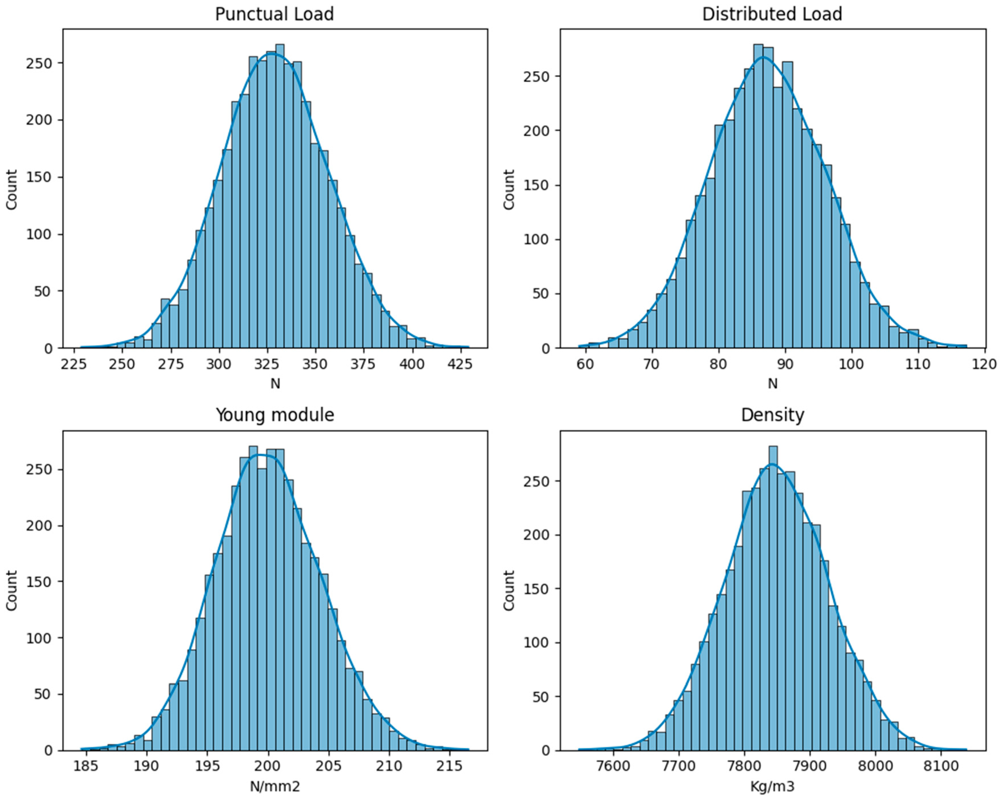
Secondly, the scalar values provided for each bridge are studied. Both their scale and distributions are taken into account to preprocess them. The distribution of the values is presented in Figure 8. The scalers tested for this task were as follows: Standard Scaler, Minmax Scaler, and Robust scalers. Among them, the scalar scaler provided the best results, which makes sense with what is seen in the data, because all values show a Gaussian distribution, and Standard Scalers are well suited for these cases.

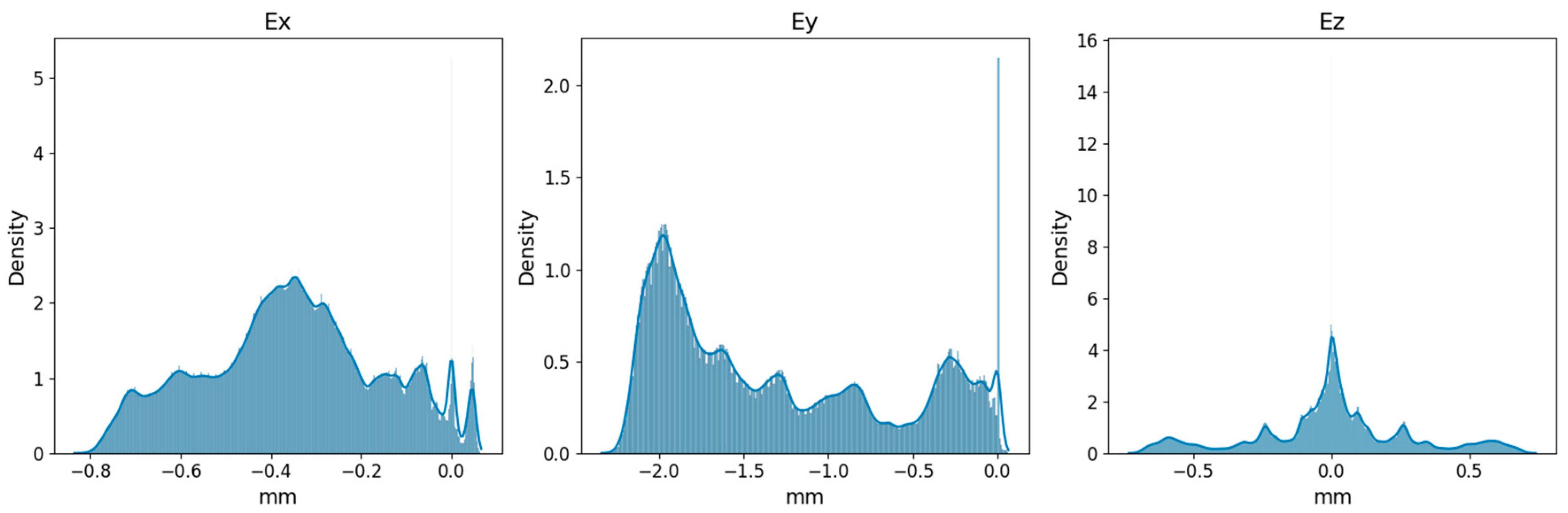
Also, the same approach was followed with the outputs, studying how they can be preprocessed to facilitate the task. Their distributions are presented in Figure 9. These distributions do not show this Gaussian behavior, and, in this case, the scaler that performs best is the MinMax Scaler.

A key concern with deep learning models is the risk of overfitting, where the model performs well on the training data but fails to generalize to new, unseen samples. Several measures were implemented to mitigate this risk.

First, regularization techniques were carried out. Early stopping was used during training, selecting the best-performing model based on validation loss. This prevents excessive training cycles that could lead to overfitting. Also, L2 weight decay was applied to the model’s parameters, discouraging overly large weight values that might indicate memorization rather than learning meaningful structural relationships.

Data augmentation was another technique used to prevent overfitting. The point clouds were randomly scaled between 0.9 and 1.1 times their size and randomly rotated around the z axis.

Finally, the model was trained during a maximum of 400 epochs, keeping the weights of the epoch that performed best in the validation split. Regarding training hyperparameters, the ones used in the original implementation of Point Transformer [24] were taken as the starting point. The largest modification was applied to the learning rate. In the original implementation, the authors used a learning rate of 0.5, with x10 reduction at 60% and 80% of the training for semantic segmentation. However, we found out that a learning rate of 0.05 provided better results in exchange for longer training time, raising from 200 epochs of the original implementation to 400. The hyperparameters used to obtain the best performance are shown in

Table 3. Training hyperparameters.

Epochs	Optimizer	Learning Rate	Momentum	Weight Decay
400	SGD	0.05	0.9	0.0001

.

4. Results

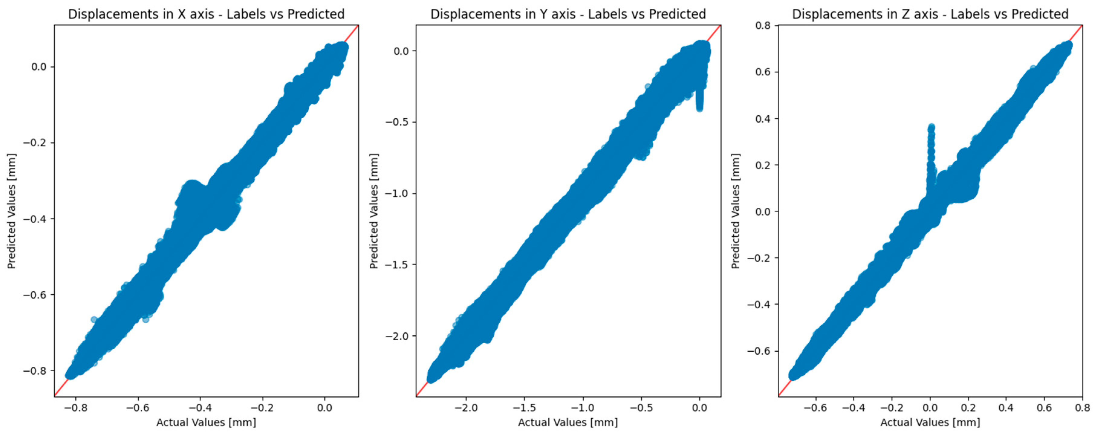
The performance of the deep learning surrogate model was rigorously evaluated using the test dataset (1000 point clouds). An example comparing the predicted displacements against the actual values is shown in Figure 10.

In this study, the two main metrics used to evaluate the performance of the surrogate model are R-squared (R²) and mean absolute error (MAE).

R-squared (R²) is a statistical measure that quantifies the percentage of the target variable’s variance that our model accounts for. In simpler terms, it measures how close the data are to the fitted regression line. The value of R² ranges from 0 to 1, where 0 means the model does not explain any of the variability in the response data around its mean, and 1 means it perfectly explains all variability. A higher R² value indicates a model that more accurately fits the observed data.

Mean absolute error (MAE), on the other hand, gives us a numerical measure of the average error per data point. The errors are calculated in mm in order to ease the understanding of this metric.

These metrics were chosen because R² provides a scale-free measure of fit, while MAE provides a direct, interpretable measure of the average error magnitude.

The tenting dataset contains 1000 samples, so the MAE and R² have been calculated for each sample, and the average over all of them are presented as the final MAE and R². Since the model provides for each point the displacements of the three axes, the metrics are also calculated three times, once per axis prediction. The results obtained are shown in

Table 4. Testing metrics.

Model	Metric	X	Y	Z
Point Transformer	R2	0.9974	0.9980	0.9984
	MAE (mm)	0.0073	0.0213	0.0086
MLP	R2	0.3988	0.3988	0.3197
	MAE (mm)	0.1211	0.4625	0.1975

.

These results indicate that R² values exceed 0.99 across all axes, demonstrating the model’s ability to account for over 99% of the variability in bridge displacements. The MAE values, measured in millimeters, were notably low, underscoring the model’s precision in predicting local displacements.

In addition, the proposed Point Transformer model has been benchmarked against a simpler MLP-based model. In contrast to the Point Transformer model, the MLP baseline obtained significantly lower R² values, below 0.4 in all axes, and higher MAE values. These results emphasize that incorporating complex spatial relationships through the transformer architecture yields substantial performance improvements over simpler surrogate models.

To provide better insight, all predicted points with the Point Transformer model have been plotted against the actual values in Figure 10. The figure shows that despite the lower MAE, the greatest errors in percentage terms are found in the z axis, with the greatest error in the test dataset at 0.407 mm.

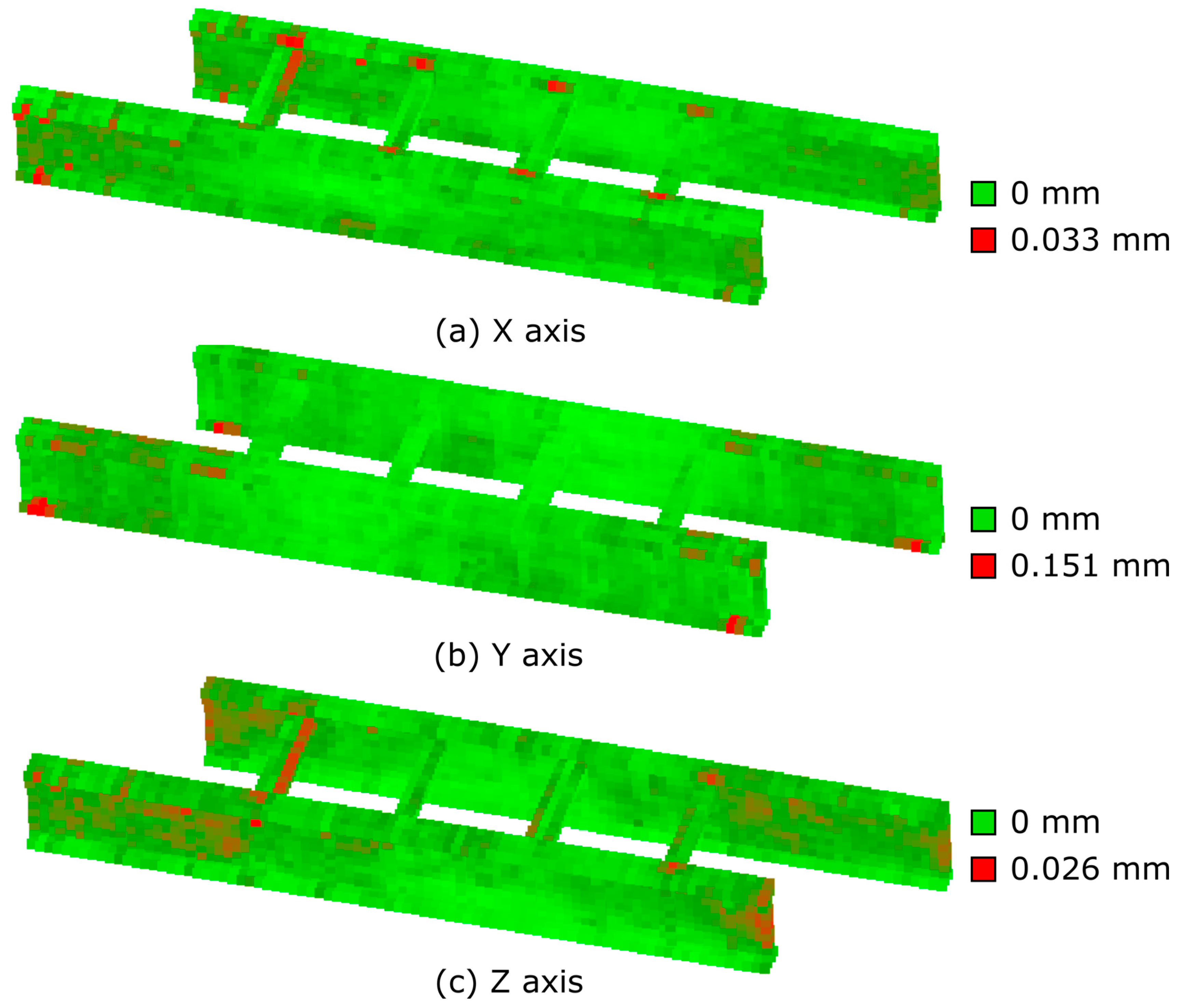
To gain further insight, the errors were mapped to their corresponding bridge coordinates. By partitioning the 3D model into 0.1 m voxels and calculating the mean absolute error within each voxel, a realistic 3D visualization of errors for each axis was generated in Figure 11. This voxel-based analysis identified regions—typically near connections and bracing elements—where geometric complexity and abrupt stiffness changes cause the model to struggle. Additionally, in areas with very high mesh density, minor mesh deformations can affect displacement values, making low-density regions more challenging.

Finally, to assess robustness under adverse conditions, experiments were conducted by introducing artificial noise to the point coordinates and simulating missing points.

Table 5. Testing metrics under measurements noise levels and missing points.

Noise (mm)	Missing Points (%)	MAE (mm)			R2
		X	Y	Z	X	Y	Z
0	0	0.0073	0.0213	0.0086	0.9974	0.9980	0.9984
0	5	0.0076	0.0223	0.0089	0.9973	0.9979	0.9983
0	10	0.0085	0.0257	0.0096	0.9968	0.9975	0.998
0	20	0.0115	0.0363	0.0121	0.9945	0.9955	0.9968
25	0	0.0078	0.0233	0.0087	0.9972	0.9976	0.9983
50	0	0.0083	0.0244	0.0092	0.9968	0.9973	0.9981
100	0	0.0099	0.0280	0.0106	0.9955	0.9961	0.9974
50	10	0.0090	0.0256	0.0099	0.9965	0.9974	0.9979

summarizes the testing metrics under various noise levels and percentages of missing points. The results indicate that while noise slightly increases the error, and substantial data loss degrades performance, the model remains sufficiently robust for practical applications.

The results shown in Table 5 show that when noise is introduced to the point coordinates, the model exhibits only a slight increase in error, indicating robust performance under typical measurement perturbations. Similarly, removing points still yields satisfactory predictions, and although performance does degrade more noticeably when a substantial portion of the data are missing, the model remains sufficiently reliable for practical use.

Overall, these observations suggest that, although accuracy naturally decreases under severe data degradation, the proposed surrogate model is resilient to moderate levels of noise or missing points, making it well suited for real-world scenarios where point clouds may be imperfect due to sensor limitations or occlusions.

5. Conclusions

Leveraging the diverse applications of deep learning in spatial data processing, this study presents a transformer-based deep learning surrogate model for bridge monitoring. Developed through extensive training on spatial data related to bridge structures, the model predicts local displacements across a bridge surface within milliseconds. It accomplishes this by incorporating key parameters such as Young’s modulus, density, load, and mesh size—the latter determining the resolution of the prediction points. By utilizing 3D point cloud data and advanced neural networks, the model efficiently captures the complex spatial relationships inherent to bridge geometry and loading conditions.

Conventionally, structural health assessments rely on manual data analysis from inspections—a labor-intensive and time-consuming approach. The deployment of a deep learning-based surrogate model represents a significant advancement, enabling the prediction of maintenance requirements and the early identification of potential issues before they escalate into serious problems. This proactive strategy enhances bridge safety and reliability while reducing maintenance costs and extending infrastructure lifespan.

Moreover, this innovative approach significantly advances traditional FE models, which, although accurate, are computationally expensive and time intensive. In contrast, the surrogate model drastically reduces the computational cost for predictions (excluding the cost of dataset generation) without sacrificing precision, offering a fast and reliable solution for structural health monitoring. Consequently, this research not only improves the efficiency of infrastructure maintenance practices but also demonstrates the transformative potential of deep learning in civil engineering.

Furthermore, applying deep learning to predict local displacements in bridges illustrates the broader potential of these technologies to foster innovation in civil engineering. By enabling real-time analysis and decision-making, deep learning supports more proactive and preventive maintenance strategies, promoting sustainable and resilient infrastructure development.

The methodology was tested on a historical steel railway bridge in Galicia, Spain. The surrogate model achieved R² values exceeding 0.99 across all axes, underscoring its robustness and precision in estimating local displacements under varying load conditions. The proposed method demonstrates the potential of deep learning technologies to revolutionize structural health monitoring (SHM) systems by rapidly processing large datasets and providing real-time predictions, thereby aiding in the identification of structural vulnerabilities for safer, more sustainable infrastructure.

The integration of our method into engineering practice is highly promising. By embedding the surrogate model into digital twin frameworks, engineers can continuously incorporate sensor data to update the bridge’s virtual replica in real time. This facilitates immediate simulation and prediction of structural responses under diverse loading conditions, thereby enabling proactive maintenance planning and rapid decision-making during emergencies. Moreover, the model’s computational efficiency allows scenario analyses to be performed in seconds—an otherwise unfeasible task with traditional FE model simulations.

However, while the proposed method shows promising results, certain limitations must be acknowledged. The model was trained and evaluated on a single steel bridge, so its direct applicability to other bridge types remains untested. Future work could explore the generalization of the model to different bridge types. Furthermore, the dataset used in this study was generated entirely via finite element simulations, ensuring controlled conditions but lacking the real-world variability typical of sensor data. To enhance practical usability, future research should test the model on point clouds acquired from laser scanning or photogrammetry, thereby incorporating real-world uncertainties.

Despite these limitations, the proposed approach represents a significant step forward in applying deep learning to structural health monitoring. Future work should also consider generalizing the model to other infrastructure types and incorporating environmental variables, such as temperature and corrosion, to further enhance predictive capabilities.