Understanding Pavement Texture Evolution and Its Impact on Skid Resistance Through Machine Learning

Abstract

The texture of asphalt pavement wears down over time due to traffic polishing, which leads to polished pavement surfaces with lower skid resistance. Three-dimensional (3D) texture parameters can be used to describe the evolution of pavement texture and establish predictive models for skid resistance. In this study, a high-resolution 3D laser scanner and a pendulum friction tester were used to collect 3D texture data and the corresponding friction values of dense-graded asphalt pavement over a period of four years. Fourier transformer and Butterworth filters were applied to decompose the 3D texture data into micro-texture and macro-texture components. Twenty different 3D texture parameters from five categories (height, spatial, hybrid, functional, and feature parameters) were calculated from pavement micro- and macro-textures and optimized using correlation methods to derive an independent set of texture parameters. The performance of a multiple linear regression model and neural network predictive model for predicting skid resistance via selected texture parameters was compared through training and testing. The results indicate that pavement micro-texture contributes more significantly to skid resistance than macro-texture, and neural network models can effectively predict the temporal evolution of skid resistance based on texture data. The neural network model achieves R² values of 0.92 and 0.89 on the training and testing sets, respectively, with RMSE values of 3.37 and 5.45, significantly outperforming the multiple linear regression model (R² = 0.50).

1. Introduction

Factors contributing to road traffic crashes are numerous and complex, including road conditions, vehicle malfunctions, weather, and driver behavior. Statistics show that over 80% of traffic crashes occur in adverse weather conditions [1], with road factors directly causing 30% of crashes and contributing directly or indirectly to 70% of accidents [2]. Research indicates that as the skid resistance of road surface improves, the probability of vehicle skidding accidents will significantly decrease [3]. Also, adverse weather like rain and snow leads to wet and slippery roads, reducing pavement skid resistance. Improper vehicle handling in such conditions increases the risk of rear-end collisions and roadway departure [4].

Pavement texture is crucial for maintaining desired skid resistance under traffic polishing. Texture evolution over time due to traffic wear and environmental factors is a key reason for changes in skid resistance [5,6]. This study aims to explore the field evolution of pavement texture and predict skid resistance based on asphalt pavement texture characteristics, which is vital for understanding how traffic polishing impacts pavement texture and friction over time.

Previous research has focused on the evolution and prediction of skid resistance using a variety of models and methods. Several studies have developed models to understand how pavement skid resistance evolves over time. For example, researchers have used logarithmic, asymptotic exponential, and S-shaped models to predict skid resistance changes based on cumulative standard axle load cycles [7,8]. Other studies have conducted wear tests on asphalt mixtures, measuring skid values and fitting decay curves using exponential functions. Moreover, some researchers have combined data from friction testers with Weibull distribution parameters to predict skid performance, while others have explored the relationship between pavement texture changes and skid resistance using three-dimensional (3D) profilometry techniques [9,10]. Additionally, accelerated wear devices and simulations of asphalt layer wear have been employed to study texture decay and build models for skid resistance prediction [11].

Despite the wealth of research on skid resistance, many studies have emphasized the importance of both macro- and micro-texture changes, noting that surface roughness parameters, such as the Hurst index and texture decay curves, are closely linked to skid resistance performance [12,13]. Zhou et al. [14] conducted abrasion tests on asphalt mixture specimens made from basalt and limestone aggregates and obtained 3D texture images at successive abrasion stages. A piece-segmented variable-dimensional method was used to characterize the changes in macro- and micro-textures. It was found that the cut-off wavelength of the function curve could be used as an index for evaluating both ordinary and differential abrasion. Also, many indoor wear tests have shown that the skid resistance of aggregates is closely related to that of asphalt pavement [12,15]. Zou et al. [16] demonstrated that 3D areal texture parameters were able to characterize macro- and micro-texture variations due to traffic polishing. The state of pavement skid resistance is also related to factors such as traffic volume, vehicle categories, environmental effects (temperature, radiation, and corrosion, etc.).

In recent years, machine learning techniques have been increasingly applied to the prediction of skid resistance, demonstrating significant improvements over traditional methods. For instance, neural network has been applied to predict sideway friction coefficient using 3D texture parameters with decent accuracy [17]. Recent studies have shown that neural network models can more effectively model the relationship between pavement texture and friction coefficient, outperforming conventional regression models in terms of accuracy [18]. Other research has explored the integration of 3D macro-texture data with traffic and environmental variables using advanced ensemble learning techniques like Bayesian optimization and LightGBM, which reduced skid resistance prediction errors by up to 28% [19]. Convolutional neural networks (CNNs) have also been employed alongside 3D texture data to predict friction levels, achieving model accuracy as high as 88% [20]. Additionally, new frameworks such as FFT-XGBoost have been developed to directly input high-resolution texture spectra into gradient boosting machines, improving prediction performance [21].

However, a review of previous studies has identified a few limitations in the evolution law of pavement texture under traffic polishing:

(1)

Most studies adopt indoor wear tests, making it difficult to truly simulate the wear of driving on the pavement, as well as the aging and erosion of pavement affected by the environment.

(2)

The time for on-site monitoring and tracking research on texture changes was relatively short, generally not exceeding two years or even mostly concentrated within one year, making it difficult to truly reflect the long-term change patterns in pavement texture.

(3)

The pavement texture characterization adopted in the research mostly employs typical 2D parameters and fractal methods, etc., which cannot comprehensively and accurately reflect changes in 3D texture.

(4)

Due to the limitations of objective factors and technical means, the research on texture evolution mostly focused on the macro-texture scale. Because the contributions of macro- and micro-texture to pavement skid resistance are different, the evolution laws of macro- and micro-texture under traffic polishing should be comprehensively evaluated.

To address these gaps, this study used a LS-40 Portable Surface Analyzer (LS-40) and a British Pendulum Tester (BPT) to collect 3D pavement texture and friction data from a field site over four years. Fourier transforms and Butterworth filters were applied to extract pavement micro- and macro-textures from the 3D texture data. Various 3D texture parameters, including height, spatial, hybrid, functional, and feature indicators, were calculated to investigate how traffic polish changes pavement texture at micro- and macro-levels. The selected texture parameters were then applied to develop pavement friction prediction models via linear regression and neural network models. This multi-faceted approach aims to explore the evolution of skid resistance, providing theoretical and technical support for predicting and evaluating asphalt pavement skid resistance.

2. Field Data Collection and 3D Texture Parameters

2.1. Field Data Acquisition

The data collection location of this study was the right travel lane of a roadway in Chengdu, China, which runs from north to south. The test section used a dense-graded AC-13 asphalt mixture, with SBS-modified asphalt and an asphalt-to-aggregate ratio of 4.6%. The designed air void content was 4.2%, and the aggregates used were basalt. The traffic volume on this road was approximately 3 million vehicles in 2018, and it has been increasing at a rate of about 10% annually since then. The layout of the field test points is shown in Figure 1. This field section was constructed with a dense-graded asphalt mixture, with basalt as the coarse aggregate, and the polished stone value of the aggregate was 53. The first data collection via LS-40 and BPT was carried out in 2018, after the road was constructed but before it was open to public traffic. Each LS-40 scan covered a 102.4 × 102.4 mm² area of the pavement surface, with a vertical resolution of 0.01 mm and a lateral resolution (x, y) of 0.05 mm. Considering that traffic wear has a long-term impact on pavement texture, and annual sampling could cover seasonal variations and the cumulative effects of traffic volume, this study adopted an annual sampling frequency to ensure data stability. Subsequently, in 2019, 2020, and 2021, another three rounds of data collection were conducted on the same spots of the field site. The test dates and ambient temperatures during the four data collections are shown in

Table 1. Test dates and ambient temperature during data collections.

No. of Data Collection	1	2	3	4
Test Date	25 May 2018	10 June 2019	4 July 2020	10 June 2021
Temperature (°C)	19–31	21–29	23–27	19–29

.

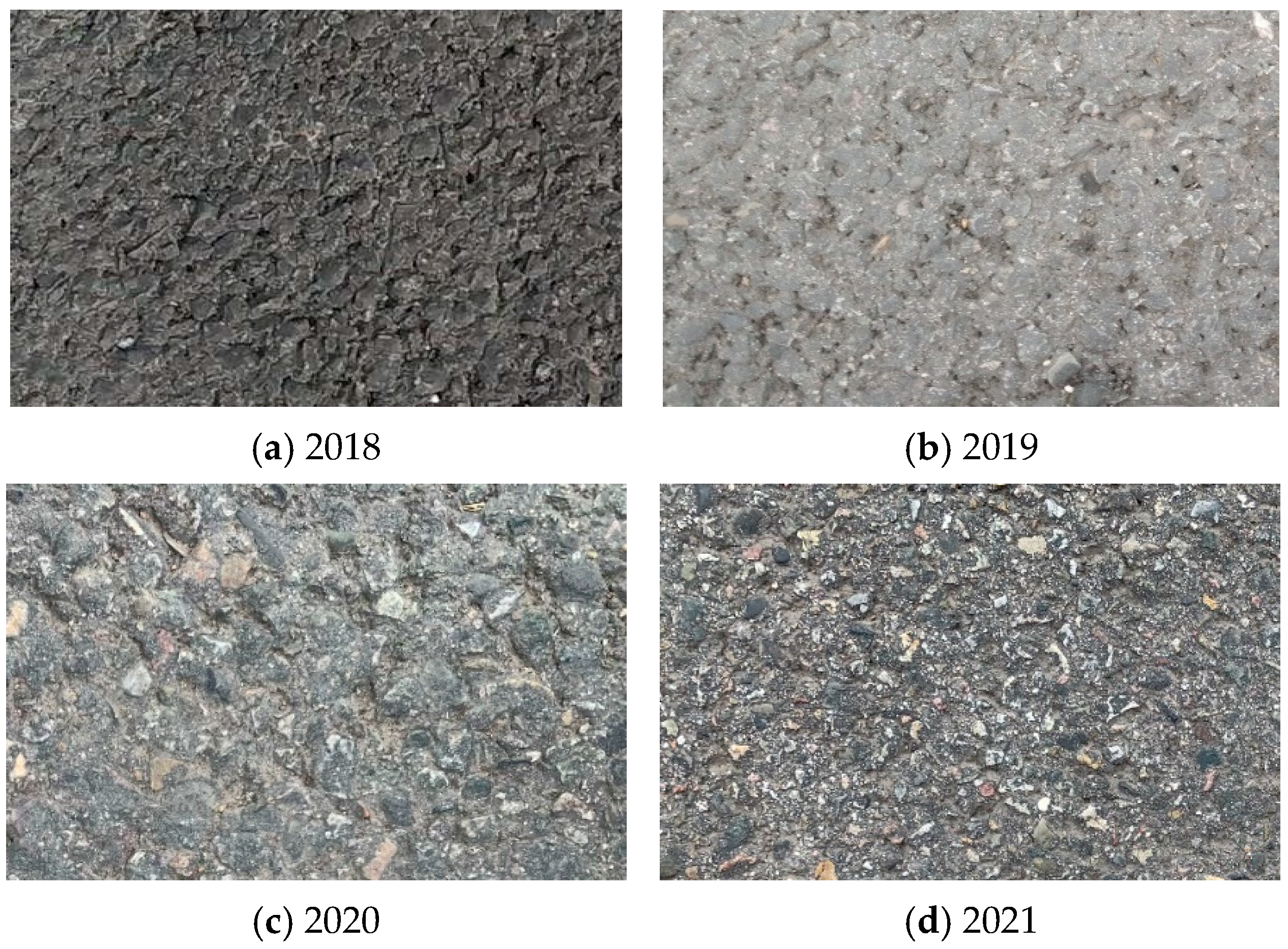
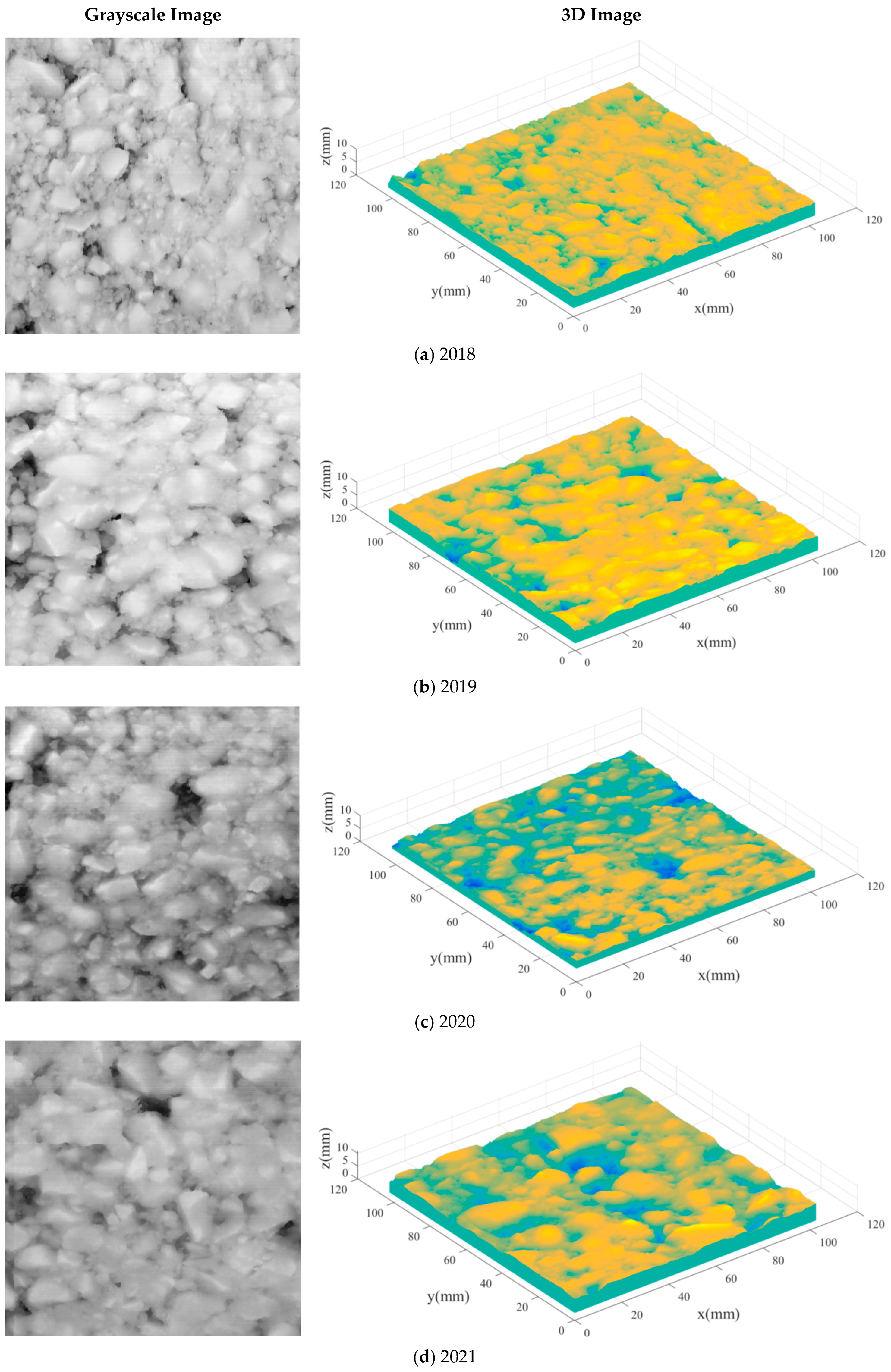
A total of 164 pairs of 3D texture and BPN (British Pendulum Number) data were collected from the four years of data collection and traffic control. Example roadway images in 2018, 2019, 2020, and 2021 during data collection are shown in Figure 2. Figure 3 presents the grayscale photos and 3D topography images of the road surface restored from LS-40 data, which better shows the changes in the road surface within four years. In Figure 3a, there were many fine aggregates and particles among the coarse aggregates on the road surface in 2018. In 2019 (Figure 3b), most of these fine aggregates had disappeared, but no significant changes were observed in the macro-texture on the surface. Figure 3c shows that the road surface in 2020 not only appeared smoother than in 2019, but also showed a little loss of coarse particles, with visible voids forming between them. By 2021, the voids between the coarse particles on the road surface had further deepened.

2.2. Three-Dimensional Texture Parameters

A Gaussian smoothing filter with a kernel size of 5 × 5 was applied to denoise the 3D texture data collected by the LS-40. Then, the Fourier transformer converted the texture height data into the frequency domain, and a Butterworth filter separated the texture components in the frequency domain into micro-texture and macro-texture, bounded at 2 Hz or 0.5 mm wavelength. Finally, the inverse Fourier transformer converted the frequency-domain micro-texture and macro-texture data into 3D texture data with height information. Details on how to obtain micro-texture and macro-texture from the LS-40 data can be found in [16].

The 3D texture data of asphalt pavement contains abundant and real texture information and features. A total of 20 3D texture parameters from five categories, including height, spatial, hybrid, functional and feature parameters, were used to describe 3D texture characteristics. Details on the calculation of 3D texture parameters can be found in [16,17]. The categories, names, and units of the 3D texture parameters used in this paper are shown in

Table 2. Three-Dimensional texture parameters.

Category		Parameters	Unit
Height Parameters		arithmetic mean height (Sa)	mm
		root mean square height (Sq)	mm
		skewness (Ssk)	-
		kurtosis (Sku)	-
Spatial Parameters		autocorrelation length (Sal)	mm
		texture aspect ratio (Str)	-
		texture direction (Std)	rad
Hybrid Parameters		root mean square gradient (Sdq)	-
		developed interfacial area ratio (Sdr)	%
Functional Related Parameters	Material Ratio Parameters	peak extreme height (Sxp)	mm
		surface section difference (Sdc)	mm
	Stratified Parameters	reduced peak height (Spk)	mm
		core height (Sk)	mm
		reduced dale height (Svk)	mm
	Volume Parameters	peak material volume (Vmp)	mm3
		core material volume (Vmc)	mm3
		core void volume (Vvc)	mm3
		dales void volume (Vvv)	mm3
Feature Parameters		peak density (Spd)	mm−2
		peak curvature (Spc)	mm−1

.

S_a and S_q measure the overall vertical roughness, with larger values indicating better water-film retention and higher friction potential at high speeds. S_sk reflects the balance between peaks and valleys, where negative values reduce hydroplaning risk and positive values improve low-speed friction. S_ku measures surface “spikiness,” with high values indicating fewer, sharper asperities that can lead to sharp friction drops when polished, serving as a polishing susceptibility indicator.

S_al and S_tr describe texture continuity, with shorter S_al and lower S_tr indicating directional traffic polishing and anisotropy in BPN20 and SFC20. Std indicates the texture orientation, with alignment to the wheel path aiding drainage and transverse alignment improving cornering grip. S_dq and S_dr correlate with surface steepness and rubber contact area, with higher values creating greater hysteresis at medium speeds.

S_xp and S_dc separate the top 2.5% of peaks, influencing tire “bite” and drainage, essential for macro-texture preservation. S_pk, S_k, and V_mp/V_mc/V_vc/V_vv stratify the surface into functional layers, tracking polishing cycles and structural fatigue, with V_mp/V_vv balance affecting water storage. S_pd and S_pc quantify stress-concentrating tips, where high values promote interlocking but also speed up aggregate fracture, helping determine when to apply anti-polishing treatments.

3. Three-Dimensional Texture Parameter Optimization

The analysis of correlations among 3D texture parameters using the Pearson correlation coefficient and associated p-values facilitates the optimization of the parameter system by identifying and eliminating redundant or highly linearly correlated texture metrics. In this study, a correlation coefficient of 0.90 indicates extremely high correlation, permitting the removal of one variable from each highly correlated pair to streamline subsequent analysis of 3D texture evolution under traffic polishing and the prediction of pavement friction via 3D texture parameters.

3.1. Correlation Analysis of Macro-Texture Parameters

Table 3. Correlation coefficients of macro-texture parameters.

Param.	Sa	Sq	Ssk	Sku	Sal	Str	Std	Sdq	Sdr	Sxp
Sa	1.00	0.97 **	−0.02	−0.07	0.20 **	0.06	0.08	0.37 **	0.36 **	0.77 **
Sq	0.97 **	1.00	−0.16 *	0.01	0.16 *	0.10	0.09	0.45 **	0.44 **	0.72 **
Ssk	−0.02	−0.16 *	1.00	−0.55 **	0.34 **	−0.12	−0.07	−0.63 **	−0.63 **	0.46 **
Sku	−0.07	0.01	−0.55 **	1.00	−0.29 **	−0.02	−0.02	0.53 **	0.53 **	−0.32 **
Sal	0.20 **	0.16 *	0.34 **	−0.29 **	1.00	−0.09	0.13	−0.40 **	−0.41 **	0.36 **
Str	0.06	0.10	−0.15	−0.02	−0.09	1.00	0.23 **	0.09	0.09	0.04
Std	0.08	0.09	−0.07	−0.02	0.13	0.23 **	1	−0.02	−0.02	0.06
Sdq	0.37 **	0.45 **	−0.63 **	0.53 **	−0.40 **	0.09	−0.02	1	1 **	−0.06
Sdr	0.359 **	0.439 **	−0.627 **	0.531 **	−0.408 **	0.092	−0.024	0.999 **	1	−0.065
Sxp	0.764 **	0.720 **	0.457 **	−0.316 **	0.360 **	0.042	0.058	−0.064	−0.065	1
Sdc	0.952 **	0.990 **	−0.183 *	0.014	0.151	0.126	0.097	0.436 **	0.428 **	0.719 **
Spk	0.261 **	0.225 **	0.536 **	−0.354 **	0.331 **	0.039	−0.017	−0.361 **	−0.359 **	0.747 **
Sk	0.934 **	0.892 **	0.203 **	−0.161 *	0.272 **	−0.001	0.071	0.219 **	0.217 **	0.827 **
Svk	0.796 **	0.890 **	−0.542 **	0.218 **	−0.004	0.151	0.094	0.610 **	0.600 **	0.396 **
Vmp	0.498 **	0.459 **	0.501 **	−0.338 **	0.364 **	0.023	0.005	−0.238 **	−0.237 **	0.870 **
Vmc	0.607 **	0.615 **	0.027	−0.130	0.186 *	0.025	0.076	0.180 *	0.170 *	0.463 **
Vvc	0.549 **	0.529 **	0.314 **	−0.162 *	0.255 **	0.018	0.076	−0.003	−0.006	0.665 **
Vvv	0.840 **	0.921 **	−0.477 **	0.174 *	0.013	0.152	0.090	0.596 **	0.585 **	0.442 **
Spd	−0.757 **	−0.704 **	−0.305 **	0.361 **	−0.172 *	−0.154 *	−0.085	0.124	0.130	−0.792 **
Spc	0.207 **	0.258 **	−0.547 **	0.519 **	−0.395 **	0.105	−0.028	0.887 **	0.892 **	−0.137

Note: Double asterisks (**) indicate that the correlation is significant at 0.01 level, and a single asterisk (*) indicates that the correlation is significant at the 0.05 level, with this convention applied consistently throughout Table 4, Table 5 and Table 6.

and

Table 4. Correlation coefficients of macro-texture parameters.

Param.	Sdc	Spk	Sk	Svk	Vmp	Vmc	Vvc	Vvv	Spd	Spc
Sa	0.952 **	0.261 **	0.934 **	0.796 **	0.498 **	0.607 **	0.549 **	0.840 **	−0.757 **	0.207 **
Sq	0.990 **	0.225 **	0.892 **	0.890 **	0.459 **	0.615 **	0.529 **	0.921 **	−0.704 **	0.258 **
Ssk	−0.183 *	0.536 **	0.203 **	−0.542 **	0.501 **	0.027	0.314 **	−0.477 **	−0.305 **	−0.547 **
Sku	0.014	−0.354 **	−0.161 *	0.218 **	−0.338 **	−0.130	−0.162 *	0.174 *	0.361 **	0.519 **
Sal	0.151	0.331 **	0.272 **	−0.004	0.364 **	0.186 *	0.255 **	0.013	−0.172 *	−0.395 **
Str	0.126	0.039	−0.001	0.151	0.023	0.025	0.018	0.152	−0.154 *	0.105
Std	0.097	−0.017	0.071	0.094	0.005	0.076	0.076	0.090	−0.085	−0.028
Sdq	0.436 **	−0.361 **	0.219 **	0.610 **	−0.238 **	0.180 *	−0.003	0.596 **	0.124	0.887 **
Sdr	0.428 **	−0.359 **	0.217 **	0.600 **	−0.237 **	0.170 *	−0.006	0.585 **	0.130	0.892 **
Sxp	0.719 **	0.747 **	0.827 **	0.396 **	0.870 **	0.463 **	0.665 **	0.442 **	−0.792 **	−0.137
Sdc	1	0.271 **	0.849 **	0.912 **	0.489 **	0.607 **	0.518 **	0.936 **	−0.696 **	0.249 **
Spk	0.271 **	1	0.289 **	−0.012	0.947 **	0.105	0.380 **	0.016	−0.489 **	−0.309 **
Sk	0.849 **	0.289 **	1	0.615 **	0.537 **	0.571 **	0.622 **	0.667 **	−0.757 **	0.079
Svk	0.912 **	−0.012	0.615 **	1	0.181 *	0.525 **	0.311 **	0.992 **	−0.454 **	0.404 **
Vmp	0.489 **	0.947 **	0.537 **	0.181 *	1	0.257 **	0.485 **	0.224 **	−0.627 **	−0.237 **
Vmc	0.607 **	0.105	0.571 **	0.525 **	0.257 **	1	0.225 **	0.552 **	−0.507 **	0.008
Vvc	0.518 **	0.380 **	0.622 **	0.311 **	0.485 **	0.225 **	1	0.344 **	−0.551 **	−0.105
Vvv	0.936 **	0.016	0.667 **	0.992 **	0.224 **	0.552 **	0.344 **	1	−0.509 **	0.388 **
Spd	−0.696 **	−0.489 **	−0.757 **	−0.454 **	−0.627 **	−0.507 **	−0.551 **	−0.509 **	1	0.233 **
Spc	0.249 **	−0.309 **	0.079	0.404 **	−0.237 **	0.008	−0.105	0.388 **	0.233 **	1

present the results of correlation analysis for macro-texture parameters. The correlation between height parameters S_a and S_q is as high as 0.97, nearly perfectly correlated, while S_sk and S_ku show no correlation with other height parameters. The spatial parameters S_al, S_tr, and S_td have very low correlation coefficients with each other, indicating no correlation. The hybrid parameters S_dq and S_dr are perfectly correlated with a coefficient of 0.99. Among the functional parameters, S_dc and S_vk are highly correlated (0.91), V_vv and S_vk are nearly perfectly correlated (0.99), and S_pk and V_mp are highly correlated (0.95). Other parameter pairs have correlation coefficients below 0.90. The feature parameters S_pd and S_pc also show no correlation.

Additionally, some parameters across different categories are correlated. For instance, the height parameter S_a is highly correlated with the functional parameters S_dc and S_k, with coefficients of 0.95 and 0.93, respectively. Similarly, the height parameter S_q is highly correlated with S_dc (0.99) and V_vv (0.92).

To reduce redundancy from highly linearly correlated macro-texture parameters, the optimized texture parameter system retains one parameter from each set of highly correlated parameters, resulting in the following configuration:

(1)

Height Parameters: S_a, S_sk, and S_ku.

(2)

Spatial Parameters: S_al, S_tr, and S_td.

(3)

Hybrid Parameter: S_dq.

(4)

Functional Parameters: S_xp, V_mp, V_mc, and V_vc.

(5)

Feature Parameters: S_pd and S_pc.

3.2. Correlation Analysis of Micro-Texture Parameters

Table 5. Correlation coefficients of micro-texture parameters.

Param.	Sa	Sq	Ssk	Sku	Sal	Str	Std	Sdq	Sdr	Sxp
Sa	1	0.936 **	0.648 **	0.523 **	0.503 **	0.824 **	0.020	0.958 **	0.960 **	0.957 **
Sq	0.936 **	1	0.776 **	0.659 **	0.633 **	0.833 **	0.011	0.989 **	0.984 **	0.992 **
Ssk	0.648 **	0.776 **	1	0.850 **	0.555 **	0.571 **	−0.057	0.702 **	0.683 **	0.718 **
Sku	0.523 **	0.659 **	0.850 **	1	0.537 **	0.491 **	−0.070	0.581 **	0.562 **	0.590 **
Sal	0.503 **	0.633 **	0.555 **	0.537 **	1	0.488 **	−0.026	0.600 **	0.587 **	0.594 **
Str	0.824 **	0.833 **	0.571 **	0.491 **	0.488 **	1	−0.061	0.854 **	0.860 **	0.841 **
Std	0.020	0.011	−0.057	−0.070	−0.026	−0.061	1	0.019	0.017	0.026
Sdq	0.958 **	0.989 **	0.702 **	0.581 **	0.600 **	0.854 **	0.019	1	0.999 **	0.994 **
Sdr	0.960 **	0.984 **	0.683 **	0.562 **	0.587 **	0.860 **	0.017	0.999 **	1	0.992 **
Sxp	0.957 **	0.992 **	0.718 **	0.590 **	0.594 **	0.841 **	0.026	0.994 **	0.992 **	1
Sdc	0.960 **	0.991 **	0.711 **	0.584 **	0.593 **	0.846 **	0.023	0.996 **	0.995 **	10.00 **
Spk	0.933 **	0.998 **	0.785 **	0.662 **	0.625 **	0.823 **	0.016	0.983 **	0.977 **	0.992 **
Sk	0.948 **	0.931 **	0.559 **	0.447 **	0.522 **	0.860 **	0.016	0.969 **	0.977 **	0.954 **
Svk	0.916 **	0.994 **	0.812 **	0.690 **	0.636 **	0.806 **	0.014	0.970 **	0.962 **	0.981 **
Vmp	0.953 **	0.941 **	0.576 **	0.462 **	0.531 **	0.861 **	0.017	0.976 **	0.982 **	0.963 **
Vmc	0.962 **	0.970 **	0.640 **	0.517 **	0.560 **	0.855 **	0.025	0.991 **	0.994 **	0.988 **
Vvc	0.928 **	0.904 **	0.520 **	0.410 **	0.500 **	0.853 **	0.016	0.948 **	0.958 **	0.930 **
Vvv	−0.805 **	−0.880 **	−0.750 **	−0.599 **	−0.455 **	−0.744 **	0.004	−0.851 **	−0.846 **	−0.876 **
Spd	0.909 **	0.948 **	0.685 **	0.559 **	0.560 **	0.841 **	0.006	0.964 **	0.964 **	0.951 **

and

Table 6. Correlation coefficients of micro-texture parameters.

Param.	Sdc	Spk	Sk	Svk	Vmp	Vmc	Vvc	Vvv	Spd
Sa	0.960 **	0.933 **	0.948 **	0.916 **	0.953 **	0.962 **	0.928 **	−0.805 **	0.909 **
Sq	0.991 **	0.998 **	0.931 **	0.994 **	0.941 **	0.970 **	0.904 **	−0.880 **	0.948 **
Ssk	0.711 **	0.785 **	0.559 **	0.812 **	0.576 **	0.640 **	0.520 **	−0.750 **	0.685 **
Sku	0.584 **	0.662 **	0.447 **	0.690 **	0.462 **	0.517 **	0.410 **	−0.599 **	0.559 **
Sal	0.593 **	0.625 **	0.522 **	0.636 **	0.531 **	0.560 **	0.500 **	−0.455 **	0.560 **
Str	0.846 **	0.823 **	0.860 **	0.806 **	0.861 **	0.855 **	0.853 **	−0.744 **	0.841 **
Std	0.023	0.016	0.016	0.014	0.017	0.025	0.016	0.004	0.006
Sdq	0.996 **	0.983 **	0.969 **	0.970 **	0.976 **	0.991 **	0.948 **	−0.851 **	0.964 **
Sdr	0.995 **	0.977 **	0.977 **	0.962 **	0.982 **	0.994 **	0.958 **	−0.846 **	0.964 **
Sxp	10.000 **	0.992 **	0.954 **	0.981 **	0.963 **	0.988 **	0.930 **	−0.876 **	0.951 **
Sdc	1	0.990 **	0.961 **	0.978 **	0.969 **	0.991 **	0.938 **	−0.870 **	0.952 **
Spk	0.990 **	1	0.917 **	0.998 **	0.928 **	0.963 **	0.888 **	−0.893 **	0.944 **
Sk	0.961 **	0.917 **	1	0.889 **	0.999 **	0.988 **	0.990 **	−0.777 **	0.915 **
Svk	0.978 **	0.998 **	0.889 **	1	0.902 **	0.943 **	0.858 **	−0.895 **	0.934 **
Vmp	0.969 **	0.928 **	0.999 **	0.902 **	1	0.992 **	0.987 **	−0.791 **	0.923 **
Vmc	0.991 **	0.963 **	0.988 **	0.943 **	0.992 **	1	0.970 **	−0.837 **	0.942 **
Vvc	0.938 **	0.888 **	0.990 **	0.858 **	0.987 **	0.970 **	1	−0.738 **	0.896 **
Vvv	−0.870 **	−0.893 **	−0.777 **	−0.895 **	−0.791 **	−0.837 **	−0.738 **	1	−0.848 **
Spd	0.952 **	0.944 **	0.915 **	0.934 **	0.923 **	0.942 **	0.896 **	−0.848 **	1

present the correlation analysis results for micro-texture parameters. S_a and S_q show a high correlation with a coefficient of 0.94. S_sk and S_ku have no correlation with other height parameters. The spatial parameters S_al, S_tr, and S_td are not correlated with each other. The hybrid parameters S_dq and S_dr are perfectly correlated (coefficient of 0.99). The functional parameters S_dc, S_xp, S_pk, S_k, V_mp, V_mc, V_vc, and V_vv are highly correlated with each other. The feature parameters S_pd and S_pc have a low correlation coefficient, below 0.90.

Some parameters across different categories are also correlated. The height parameter S_a is highly correlated with the hybrid parameters S_dq and S_dr, as well as the functional parameters S_dc, S_xp, S_pk, S_k, V_mp, V_mc, V_vc, V_vv, and the feature parameter S_pc.

Based on these results, the micro-texture parameter set can be optimized to: S_a, S_sk, S_ku, S_al, S_tr, S_td, and S_pd.

4. Evolution of 3D Texture Under Traffic Polishing

To explore the evolution of the macro- and micro-texture of road surfaces under traffic and environmental influences, this study analyzed 164 sets of 3D texture data collected over four consecutive years. Using the proposed methods for calculating height, spatial, hybrid, functional, and shape parameters for both macro- and micro-textures, the study investigated the changes in previously selected parameters, characterizing the texture evolution under traffic polishing. Traffic polishing is divided into overall and differential wear. Overall wear refers to the phenomenon where the pavement surface undergoes uniform wear under the action of vehicle loads. This type of wear manifests as the gradual stripping and reduction in surface materials, leading to a decrease in the overall height of the pavement, typically distributed evenly across the entire surface. Overall wear focuses on the total amount of wear across the entire surface. Differential wear refers to the non-uniform wear that occurs between different areas or different materials on the pavement surface under the action of vehicle loads. This type of wear usually presents as severe wear in some areas and lighter wear in others, resulting in significant wear differences across the surface. Differential wear focuses on the wear differences between localized areas of the surface.

4.1. Macro-Texture Evolution

4.1.1. Height Parameters: S_a, S_sk and S_ku

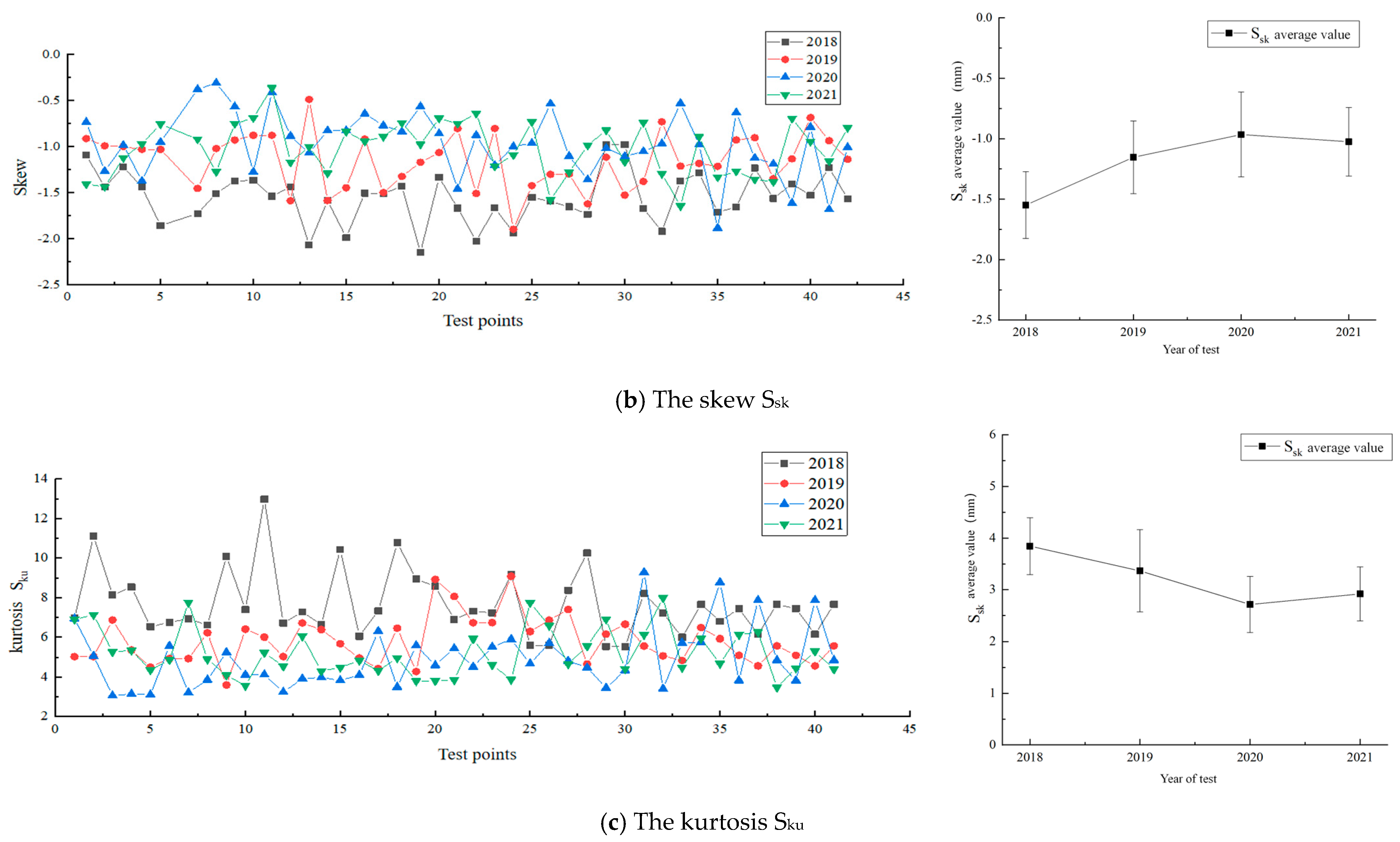
Changes in the height parameters of the macro-texture of the dense-graded asphalt pavement are shown in Figure 4. In Figure 4a, changes in the arithmetic mean height (S_a) of macro-texture over the years show no clear distinction. Assessing overall changes using mean and standard deviation in the right-side figure reveals a slight drop in S_a after the first year of traffic (−2.3%), but small increases in the second and third years (5% and 2.8%, respectively). S_a reflects overall height changes in macro-texture. Combined with 3D morphology changes, it is inferred that the initial S_a decrease was due to fine aggregate and asphalt membrane stripping from wear and environmental effects. In the following two years, differential wear led to an increase in S_a.

In Figure 4b, the skewness (S_sk) of macro-texture is consistently negative, indicating a negative texture with valleys deeper than peaks. Figure 4c shows that S_sk increased over the first two years, with the mean rising from −1.55 to −0.97 (25.5% and 16.3% increases), but the rate of increase slowed yearly. In the next two years, S_sk remained largely unchanged, with a minor mean decrease of 0.05 (−6.1%). This suggests that traffic polishing reduces the negative texture structure. In the first two years, fillers between coarse aggregates were stripped, and valley areas were filled, weakening the negative texture. However, between 2020 and 2021, traffic polishing and environmental effects mainly impacted the coarse aggregates, leading to minimal macro-texture changes and small overall S_sk variations.

Dense-graded asphalt pavement has a pronounced kurtosis structure. As shown in Figure 4c, the kurtosis (S_ku) averaged above 3 each year. S_ku decreased continuously over the first three years, from 7.68 to 4.92 (−24.1% and −15.6% decreases), with minimal change in the fourth year (+6.1%). The S_ku decline indicates an increase in mid-height probabilities and a decrease in extreme height probabilities. For negatively textured pavement, this means fewer extremely low heights in the valleys.

4.1.2. Spatial Parameters: S_al, S_tr, and S_td

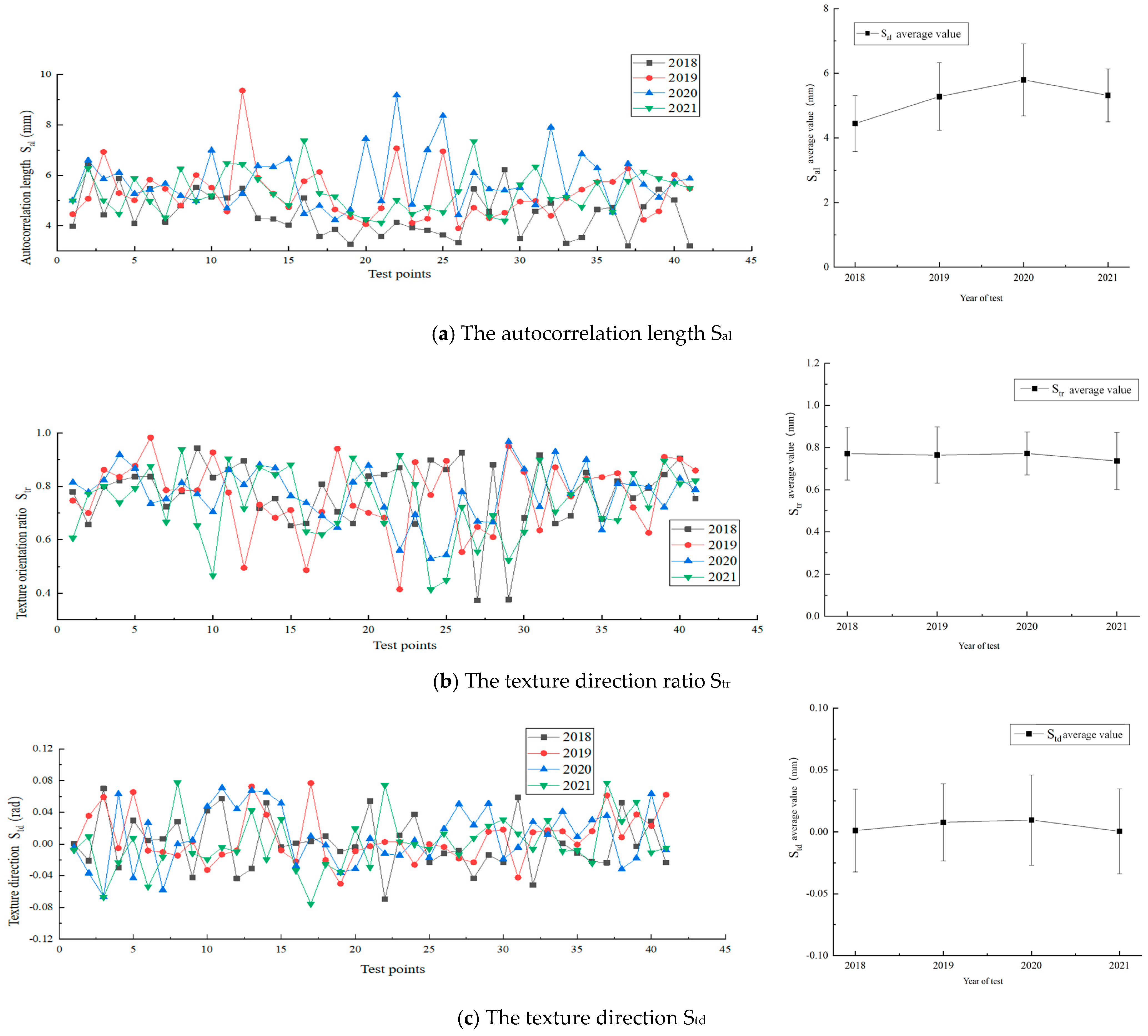
The variation in the macro-texture spatial parameters of dense-graded asphalt pavement under traffic and environmental effects is shown in Figure 5. The autocorrelation length (S_al) of macro-texture changed in two phases. From 2018 to 2020, S_al increased from 4.44 mm to 5.79 mm (15.8% and 9.7% increases). After 2020, it decreased to 5.31 mm (−8.3%). S_al reflects the minimum horizontal shift in the macro-surface with the same correlation. In the first phase, overall wear gradually removed the surface asphalt membrane and fine aggregates, exposing coarse aggregates and lengthening S_al. In the second phase, differential wear of coarse aggregates reduced their size, thus shortening S_al.

As shown in Figure 5b, the texture direction ratio (S_tr) remained stable over four years, averaging around 0.77 in the first three years and slightly dropping to 0.74 (−4.6%) in the fourth year. S_tr measures the anisotropy of macro-texture and the ratio of maximum to minimum autocorrelation lengths of coarse aggregates. Despite varied coarse aggregate shapes, the macro-texture showed some isotropy. In the early stage, overall wear did not alter the overall shape of coarse aggregates, so S_tr remained stable. Later, differential wear began to change the coarse aggregate shape, but due to its short duration, S_tr only slightly decreased. The macro-texture direction (S_td) fluctuated around 0 rad, with a standard deviation below 0.05 rad (Figure 5c), indicating that the macro-texture direction is insensitive to wear, which is related to the isotropic nature of the macro-texture.

4.1.3. Hybrid Parameters: S_dq

The S_dq values show a clear distinction between years, decreasing from 0.79 in the first year to 0.35 in the third year (a 47.3% and 16.0% reduction), indicating that the overall slope of the macro-surface dropped by half from 38.3 to 19.2, and then remained unchanged, as shown in Figure 6. It indicates that the surface flatness and complexity of the macro-texture underwent two phases of change:

Rapid Decline Phase: The easily worn surface layer was quickly removed by the combined effects of traffic and the environment, leading to a fast reduction in flatness and complexity.

Equilibrium Phase: At this stage, the wear and environmental effects could no longer significantly alter the overall flatness of the macro-surface.

4.1.4. Functional Parameters: S_xp and S_dc

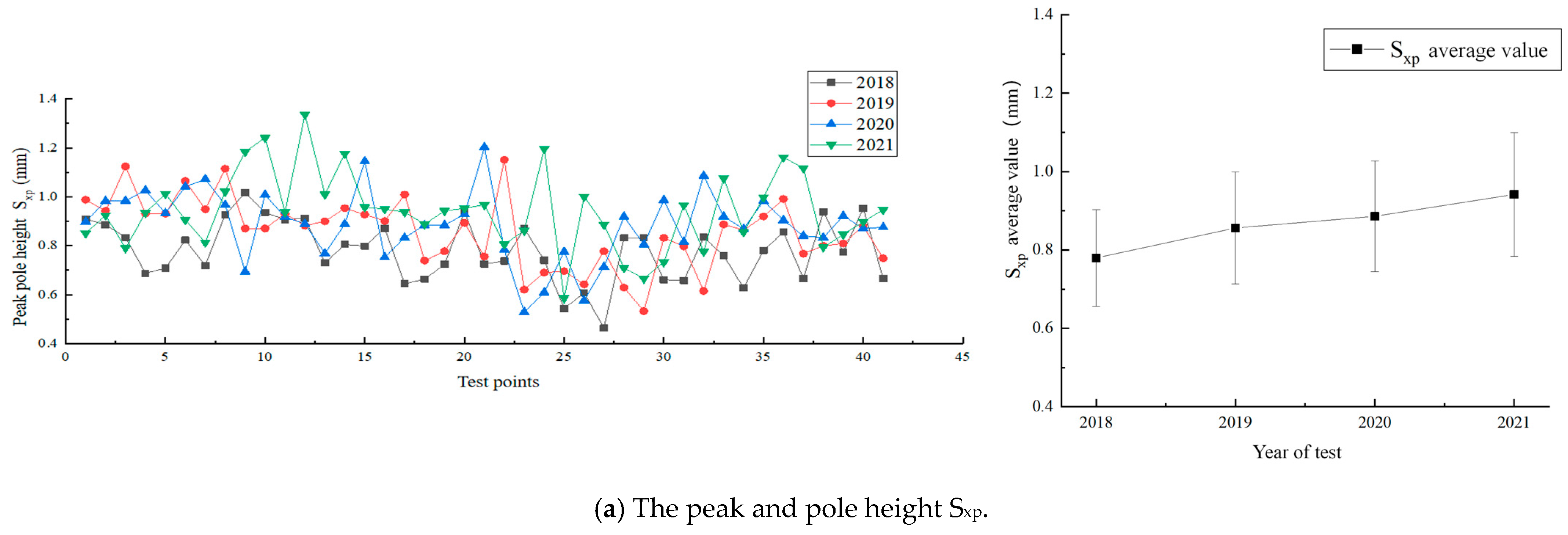
The variation in macro-texture material ratio parameters of the pavement is shown in Figure 7. In Figure 7a, the peak height (S_xp) exhibits a yearly increasing trend, with the mean value rising from 0.78 mm in 2018 to 0.94 mm in 2021 (increases of 9.8%, 3.4%, and 6.3%, respectively).

Figure 7b shows that the surface profile height difference (S_dc) undergoes two phases of change: a decrease followed by an increase. In the first phase, the mean S_dc slightly decreased from 2.67 mm in 2018 to 2.58 mm in 2019 (−3.4%) and remained unchanged from 2019 to 2020. In the second phase, the mean S_dc increased from 2.59 mm in 2020 to 2.77 mm in 2021 (increases of 3.4% and 6.5%).

This indicates that during the overall wear phase, the filling of valleys reduced the overall profile height difference. However, by the third year, differential wear caused coarse aggregate loss, expanding the overall profile height difference. S_xp, representing the upper portion height difference, shows a consistent increase due to traffic wear, suggesting that the upper part of the surface texture is continuously growing. Considering the limited overall height change in the profile, the proportion of the upper part’s height to the entire surface is steadily increasing.

4.1.5. Feature Parameters: S_pd and S_pc

The variation in macro-texture feature parameters characterizes the morphological changes at the peaks, including peak density and curvature, which significantly impact friction, as they are stress concentration areas contacting tires. The overall and statistical analysis of these parameters for the measured road section is shown in Figure 8. As depicted in Figure 8a, the peak density (S_pd) exhibits a continuous downward trend, decreasing from 0.3 per mm² in 2018 to 0.25 per mm² in 2021. The first year saw the most significant reduction of 0.03 per mm² (−8.6%), followed by smaller decreases of 0.01 per mm² in the next two years (−4.8% and −3.9%). This indicates that initial wear had the most substantial impact on peak density, with subsequent wear having a smaller effect, yet the overall trend remains a decrease.

Figure 8b shows that the peak curvature (S_pc) also decreased significantly, with a 26.4% drop in the first year. Thereafter, it continued to decrease by about 7% annually in a linear fashion. This suggests that the initial overall wear had a more pronounced effect on S_pc compared to differential wear in later years.

From the perspective of shape parameters, overall wear has a more significant impact on peak morphology. The first year’s overall wear primarily affected the finer aggregates adhering to and filling the spaces between coarse aggregates, which are more susceptible to wear. This resulted in marked decreases in both peak density and curvature. In the following two years, the rate of decrease slowed as overall wear had a less pronounced effect on the coarse aggregate surfaces. However, the trend of decreasing peak density and curvature continued without reaching an equilibrium point over the four years, which is distinctly unfavorable for the skid resistance of the pavement.

4.2. Micro-Texture Evolution

Micro-texture, as the primary contact interface between pavement and vehicle tire, significantly impacts skid resistance. Consistent with the approach in Section 4.1, this section uses 3D texture parameters to provide a comprehensive characterization of micro-texture evolution under traffic wear and environmental effects. The micro-texture data points in this section are directly aligned with the macro-texture data points presented in the previous section, ensuring a cohesive analysis across scales.

4.2.1. Height Parameters: S_a, S_sk and S_ku

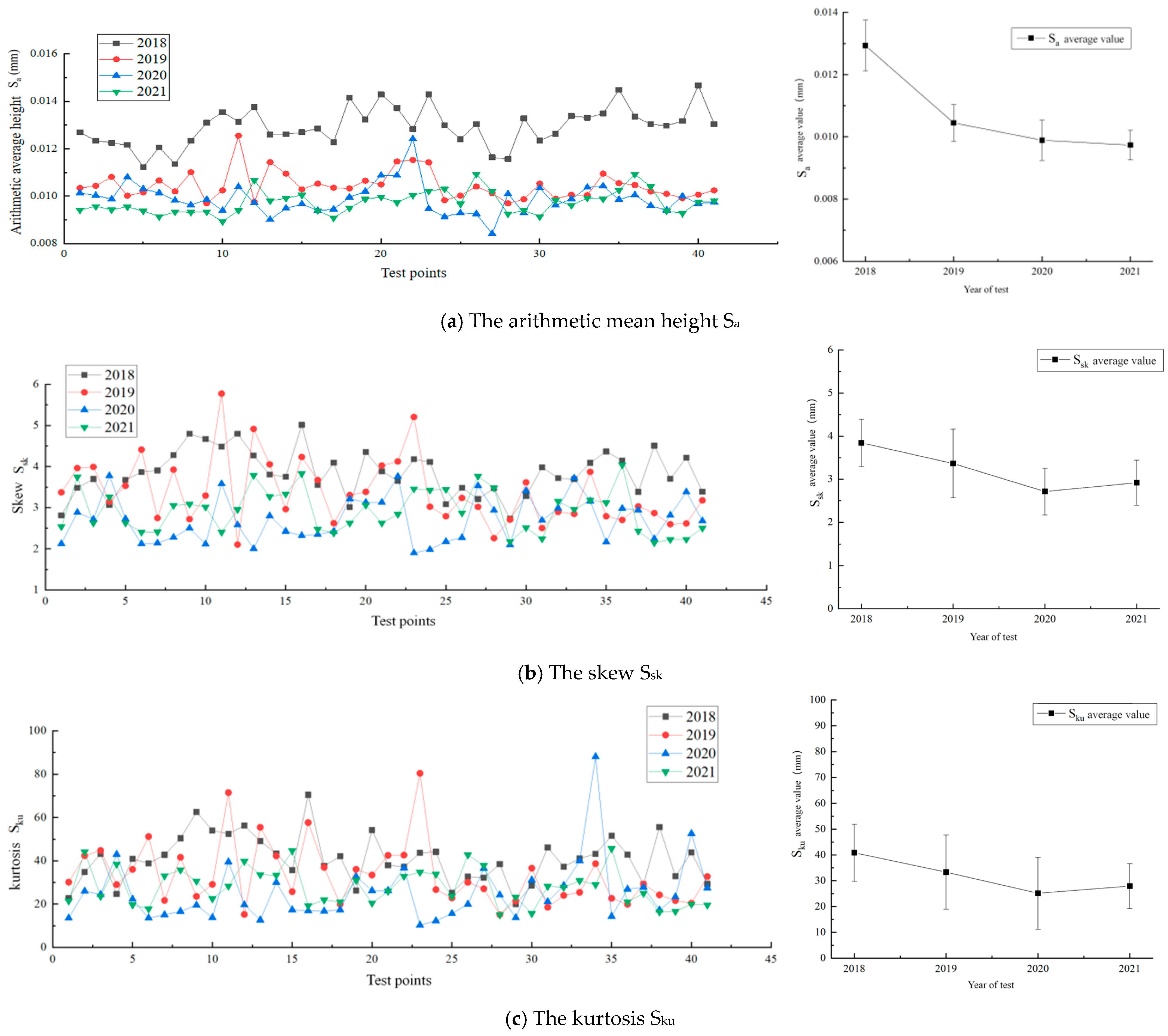
Changes in the height parameters of the micro-texture in dense-graded asphalt pavement are shown in Figure 9. In Figure 9a, the arithmetic mean height (S_a) of the measured points shows clear distinctions over the years, with significant declines from 2018 to 2019. Statistical analysis (right-side figure) reveals a substantial 20% drop in the first year (from 0.13 mm to 0.10 mm), followed by smaller annual decreases (−5.4% and −1.5%). The overall downward trend in the mean curve resembles an inverse proportion curve, indicating a weakening effect of wear on micro-texture, which is unfavorable for skid resistance. However, by 2021, the changes in S_a reached an equilibrium point.

Figure 9b shows that the skewness (S_sk) of the micro-texture is positive, indicating a positive texture with pronounced protrusions, beneficial for tire–pavement contact. However, from 2018 to 2020, S_sk values decreased linearly from an average of 3.8 to 2.7 (−12.5% and −19.4%), suggesting that traffic wear weakens the positive micro-texture structure. From 2020 to 2021, S_sk stabilized with a slight increase of 0.2 (7.6%), indicating that upper heights further from the mean surface are more susceptible to wear and erosion.

As shown in Figure 9c, the kurtosis (S_ku) of micro-texture is significantly higher than 30, with a minimum average around 25. S_ku decreased continuously over the first three years, from 40.9 to 25.2 (−18.4% and −24.5%), and stabilized in the fourth year. The reduction in kurtosis suggests a decrease in the probability density of extremely high points on the peaks.

4.2.2. Spatial Parameters: S_al, S_tr, S_td

The variation in micro-texture spatial parameters of dense-graded asphalt pavement under traffic and environmental effects is shown in Figure 10. As shown in Figure 10a, the autocorrelation length (S_al) of the micro-texture changed in two phases. From 2018 to 2020, S_al rapidly decreased from 0.2 mm to 0.05 mm (−62.3% and −36.7%). After 2020, the autocorrelation length (S_al) increased to 0.17 mm (240%). The average S_al of the micro-texture was only 1/20th of that of the macro-texture, consistent with its scale. This trend indicates that traffic wear significantly affects the horizontal properties of micro-texture, with S_al influenced by both overall and differential wear.

Figure 10b shows that the texture direction ratio (S_tr) decreased rapidly over the four years, from an average of 0.83 in 2018 to around 0.1 in 2021 (−50.4%, −27.6%, and −66.8%). The texture direction standard deviation (S_td) fluctuated around 0 rad, but with a decreasing annual standard deviation (Figure 10c). S_tr, defined as the ratio of the minimum to maximum autocorrelation lengths, indicated that new pavement has some isotropy, but wear quickly makes it anisotropic. To better understand these changes, boundary projections at an autocorrelation coefficient of 0.2 for each year are shown in Figure 11. The projections show that tire wear in a single traffic direction lengthens the autocorrelation projection along the traffic direction while changing little in the perpendicular direction. Additionally, wear makes the micro-texture direction more aligned with the traffic direction, reducing the standard deviation of the texture direction over time.

As depicted in Figure 10b, some S_tr values approached zero in 2020, with a substantial proportion nearing zero by 2021. This trend indicates a significant horizontal spatial evolution of micro-texture, specifically manifesting as texture stripping. As shown in Figure 12, the micro-texture in 2021 exhibited clear and distinct stripping along the traffic direction, a marked change compared to the data in 2018. The stripping of micro-texture aligns with the traffic direction, which may lead to differences in longitudinal and transverse skid resistance after years of wear.

4.2.3. Hybrid Parameters: S_dq

The changes in the hybrid parameters of the micro texture are shown in Figure 13. As can be seen from the left graph, the trend of the root mean square gradient S_dq is consistent with the changes in the hybrid parameters of the macro texture. From the statistical graph on the right, it can be observed that the average value of S_dq shows an inverse-proportional decreasing trend, but the rate of decline decreases year by year. By the third year, the decline trend becomes very gentle, reaching a balance point. The value of S_dq ranges from 0.16 in 2018 to 0.09 in 2021 (−33.4%, −11.4%, −2.7%). Thus, the hybrid parameters exhibit a similar change pattern, a rapid decline in the early stage and then gradually reach a balanced state.

4.2.4. Functional Parameters: S_xp

The changes in the functional parameters of the micro-texture are shown in Figure 14. The peak point height S_xp in the figure shows a decreasing inverse proportional trend year by year, and the rate of decrease shows a trend of gradually slowing down. Finally, the curve becomes relatively flat in 2021. The average value of S_xp decreases from 0.051 mm in 2018 to 0.037 mm in 2020 (−20.6%, −7.6%), the average value in 2021 remains at this value, and the standard deviation shrinks. The upper part of the micro-texture has a large proportion of the total height difference of the entire micro-texture cross-section, exceeding 70% over the years. Additionally, the proportion of the reduction in the height difference in the upper part represented by S_xp is around 27%, indicating that the micro-texture is affected by vehicle wear and environmental factors. This is different from the rule that the wear of the macro-texture mainly occurs at the peak and core parts.

4.2.5. Feature Parameter: S_pd

As illustrated in Figure 15, the peak density (S_pd) of the micro-texture first increased and then stabilized. The average S_pd rose slightly from 1.025 per mm² in 2018 to 1.069 per mm² in 2020 (2.1% each year) and remained unchanged in 2021. This increase in peak density is likely due to overall wear removing the asphalt layer and exposing the surface of coarse aggregates, with the increased S_pd originating from the micro-texture of coarse aggregates. Once the coarse aggregate surfaces were fully exposed, the peak density stopped increasing.

The removal of asphalt and fine aggregates attached to the surface of coarse aggregates in the first year of overall wear had the greatest impact. Subsequent overall wear had a slower effect on the micro-texture of the coarse aggregate surfaces. Therefore, the rate of change of the peak density and curvature slowed down, with feature parameters showing a trend towards equilibrium by 2021.

5. Prediction of Pavement Friction via 3D Texture Parameters

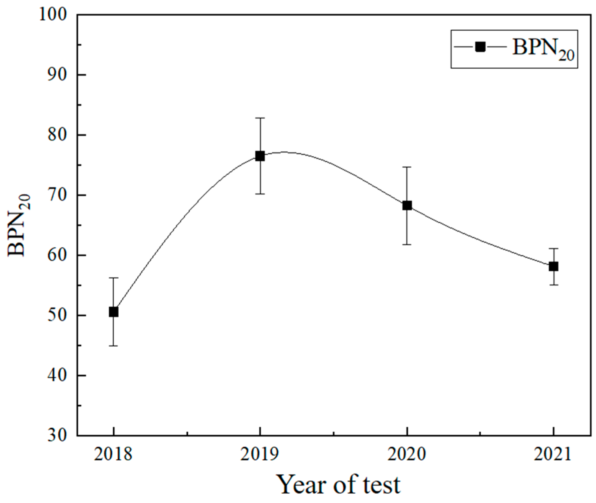
This section explores the possibility of developing pavement friction prediction models via selected 3D texture parameters at macro- and micro-levels. As shown in Figure 16, the skid resistance (BPN) of this site initially rises rapidly, peaks after the first year of wear, and then declines gradually but at a slower rate. In this study, multiple linear regression and neural network models are trained and compared on the prepared dataset to select the best model for non-contact friction estimation.

5.1. Multiple Linear Regression Model

The BPN refers to the number measured by a pendulum-type friction coefficient tester to determine the pavement friction coefficient to evaluate pavement skid resistance. The measurement results of the pendulum-type friction tester are affected by ambient temperature during field testing. Therefore, it is stipulated that the measured BPN should be corrected to a standard temperature of 20 °C. The correction method is shown in Equation (1) [22].

$${BPN}_{20}={BPN}_t+∆BPN$$

(1)

where ${BPN}_{20}$ is the pendulum number at the standard temperature of 20 °C; ${BPN}_t$ is the pendulum number measured at the ambient temperature of t °C; $∆BPN$ is the temperature correction value, as listed in

Table 7. Summary of temperature correction values.

Temperature (°C)	0	5	10	15	20	25	30	35	40
$∆\mathit{B}\mathit{P}\mathit{N}$	−6	−4	−3	−1	0	+2	+3	+5	+7

Note: The intermediate $∆BPN$ is determined by interpolation.

[22]. For instance, when ambient temperature is 30 °C, Table 7 gives ΔBPN = +3, the BPN₂₀ would be equaled to BPN₃₀ + 3.

To analyze the multiple linear relationships between the 3D texture parameters and BPN₂₀, the collected 164 pairs of 3D textures and BPN₂₀ over the years were randomly divided into a modeling group and a testing group in a 7:3 ratio. Seventy percent of the data formed the modeling group for regression model training. The model’s performance and accuracy were assessed using common regression metrics: the coefficient of determination (R²) and the Root Mean Square Error (RMSE).

To compare the effects of macro- and micro-textures on BPN₂₀, three regression models were constructed as follows:

$${BPN}_{20}={\beta }_1+{\beta }_{macro1}{X}_{macro}$$

(Model 1)

$${BPN}_{20}={\beta }_2+{\beta }_{micro2}{X}_{micro}$$

(Model 2)

$${BPN}_{20}={\beta }_3+{\beta }_{macro3}{X}_{macro}+{\beta }_{micro3}{X}_{micro}$$

(Model 3)

Models (1), (2), and (3) present multiple regression analysis models based on 3D texture parameters from macro-texture only, micro-texture only, and both macro- and micro-textures, respectively. Coefficients of texture parameters in these models are listed in

Table 8. Coefficients of multiple linear regression models.

Texture Parameters		Model 1: Macro- Only	Model 2: Micro- Only	Model 3: Macro- and Micro-
Macro-texture parameters	Sa	−19.24		−33.74
	Ssk	−0.30		2.20
	Sku	−0.96		−0.62
	Sal	3.20		2.93
	Str	7.73		2.29
	Std	−2.91		−36.80
	Sdq	−33.94		−8.35
	Sxp	47.18		−1.01
	Vmp	−1654.13		−408.28
	Vmc	−24.24		−15.70
	Vvc	−7.90		5.82
	Spd	−48.06		−142.50
	Spc	982.83		85.32
Micro-texture parameters	Sa		−6795.25	−5548.24
	Ssk		2.10	0.89
	Sku		0.14	0.13
	Sal		−92.93	−73.39
	Str		12.34	18.02
	Std		140.74	103.25
	Spd		−145.96	−201.51
intercept		66.11	285.36	388

, and model performance and prediction evaluations are shown in

Table 9. Multiple linear regression model evaluation.

Multiple Linear Regression Models	Model Training		Model Testing
	R2	RMSE	R2	RMSE
Model 1. Macro- only	0.20	8.95	0.03	11.97
Model 2. Micro- only	0.37	7.20	0.29	10.61
Model 3. Macro- and micro-	0.50	6.43	0.30	11.87

. Model 3, with 3D parameters from macro- and micro-texture, shows the best fit, with an R² of 0.5 and the lowest RMSE, surpassing Model 1 (macro-texture, R² = 0.20) and Model 2 (micro-texture, R² = 0.37). When using the other 30% of the data for model testing, the R² and RMSE of Model 3 match those of Model 2 but outperform those of Model 1. This indicates that both macro- and micro-textures influence BPN₂₀, with micro-texture playing a larger role, likely due to the predominance of adhesive effects during BPT measurement.

However, the best model (Model 3) only achieves an R² of 0.5 for model training, indicating a moderate fit, and an R² of 0.3 for model testing. This implies a nonlinear relationship between 3D texture parameters and BPN₂₀, suggesting that further exploration of nonlinear relationships is needed.

5.2. Neural Network Model

This section develops a BPN₂₀ prediction model via 3D macro- and micro-texture parameters using neural networks. Feedforward neural networks (FFNNs), the most widely used artificial neural networks, can solve complex nonlinear problems with basic math operations. Adequate neuron layers allow FFNNs to estimate any complex nonlinear continuous function, but the relationship between neuron layers and approximation accuracy remains unclear. Via trial-and-error, setting 10 hidden neurons achieved high prediction accuracy [23]. FFNNs have been applied in image-based pavement distress detection and offer advantages like parallel computing, high fault tolerance, and self-learning [24,25,26]. Compared to models such as support vector machines and random forests, neural networks have a stronger ability to approximate multi-variable nonlinear mappings. Existing studies have also shown that they perform excellently in texture-friction modeling [17,21].

This study used FFNN, with a structure consisting of an input layer (20 texture parameters), a hidden layer (10 neurons, with a tan-sigmoid activation function), and an output layer (BPN20). The training employed the Levenberg–Marquardt algorithm, and the dataset was split into training, validation, and testing sets with a ratio of 7:1.5:1.5. To prevent overfitting, an early stopping strategy (validation stop) was used, and the number of training epochs was limited to a maximum of 1000.

As in Section 5.1, three models were formed based on different texture parameter categories. Model 4 and Model 5 include macro- only and micro- only texture parameters, respectively, while Model 6 combines both macro- and micro- texture parameters. Based on considerations such as the requirements for model training and evaluation, the rationality of data volume and proportion, as well as the prevention of data leakage and evaluation bias, the 164 pairs of texture-friction data were randomly split into training (70%), validation (15%), and testing (15%) samples. This division not only ensures an adequate number of training samples, allowing the model to fully learn data features, but also guarantees that the validation and test samples are representative, enabling effective monitoring of model performance and objective assessment of its generalization ability. At the same time, it reduces the risk of data leakage, making the evaluation results more stable and reliable, and providing a scientific and reasonable database for the development, optimization, and evaluation of the model. The validation set was used for cross-validation and to ensure generalization, stopping training when generalization ceased improving. Through cross-validation, early stopping, limiting the number of hidden layer neurons (10), and regularization, overfitting was effectively avoided. The test set, using independent-of-model-development data, evaluated model performance using R² and RMSE. Results are compared in

Table 10. Analysis results of neural network model.

Neural Network Model	Model Training		Model Sample
	R2	RMSE	R2	RMSE
Model 4. Macro- only	0.69	6.18	0.62	8.03
Model 5. Micro- only	0.77	5.25	0.72	6.15
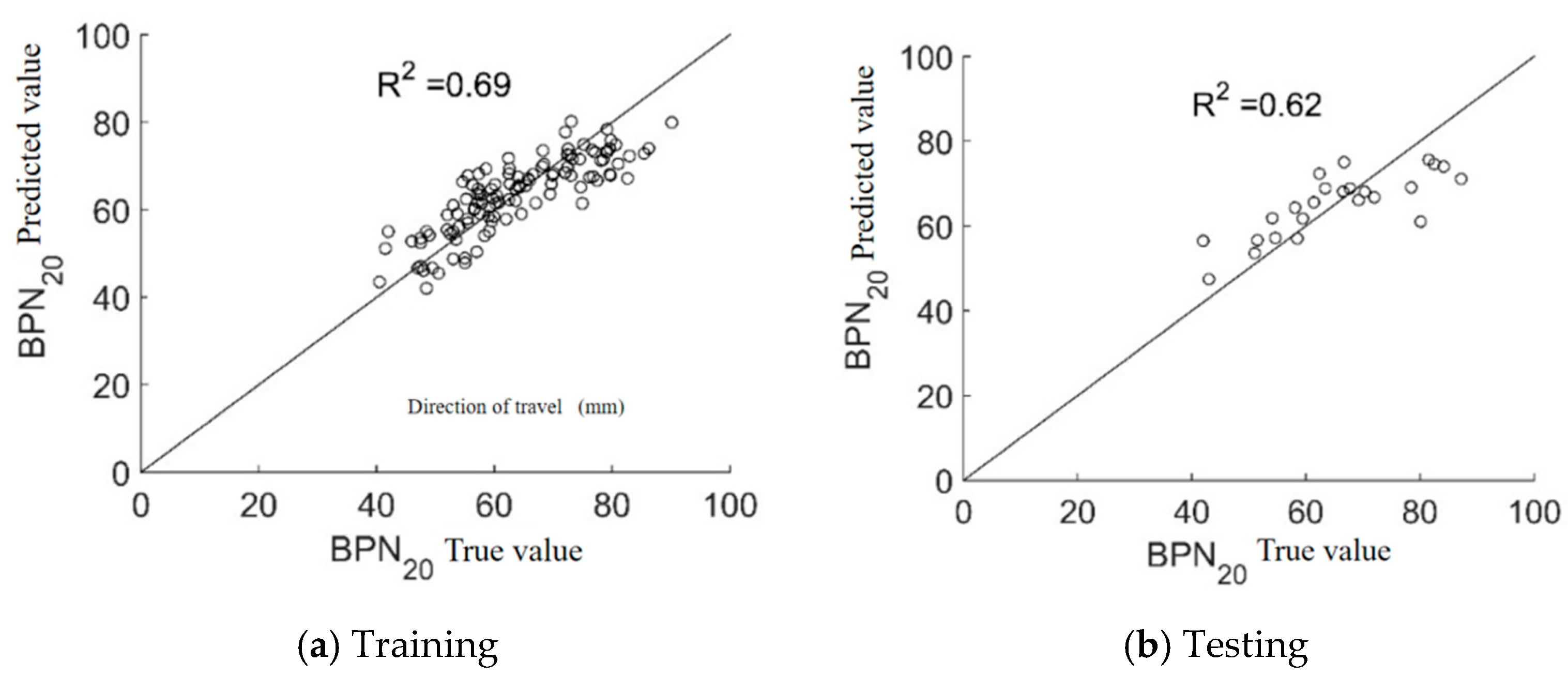
Model 6. Macro- and Micro-	0.92	3.37	0.89	5.45

, with training and testing results plotted in Figure 17, Figure 18 and Figure 19.

Comparing the R² and RMSE values of the three models, Model 6, which includes both macro- and micro-texture parameters, outperforms Model 4 (macro- only) and Model 5 (micro- only) in both training and testing datasets. Model 6 achieves R² values of 0.92 (training) and 0.89 (testing), with RMSE values of 3.37 and 5.45, respectively. These results indicate that the FFNN effectively models the nonlinear relationship between the optimized 3D texture parameters and BPN₂₀-based skid resistance, showing excellent generalization. Comparing the neural network and multiple linear regression models, it is clear that the relationship between 3D texture parameters and BPN₂₀ is nonlinear. Moreover, Model 5 (micro- only) shows better training and prediction performance than Model 4 (macro- only). Among the micro-texture parameters, S_a, S_dq, and S_pd contribute the most to BPN20 prediction (accounting for 18.3%, 15.7%, and 12.4%, respectively). Among the macro-texture parameters, S_xp and V_mp have relatively higher contributions (11.2% and 9.8%, respectively). These results are consistent with theoretical analysis and further validate the dominant role of micro-texture in low-speed skid resistance. This suggests micro-texture evolution has a more significant impact on BPN₂₀ changes.

6. Conclusions

This study provides a comprehensive understanding of how asphalt pavement texture evolves under traffic polishing and how these changes impact skid resistance. A total of 164 sets of 3D texture and BPN data were collected from a dense-graded asphalt pavement over a four-year period. Fourier–Butterworth filtering was applied to separate macro- and micro-texture components. Twenty 3D texture parameters across five categories were computed to characterize surface features. Through correlation analysis, the initial 40 indicators were reduced to 20 independent parameters. Texture evolution under traffic polishing was examined by tracking these parameters over time. The dataset was split into training and testing sets, and both multiple linear regression and neural network models were developed to predict skid resistance. Key findings include:

(1)

Parameter Optimization: Correlation analysis eliminated redundant indicators, yielding 13 macro-texture and 7 micro-texture parameters. This optimized set ensured independence and representativeness for modeling.

(2)

Texture Evolution: Traffic polishing caused a two-stage evolution in texture. At the macro scale, S_a decreased then stabilized, S_al rose then fell, and S_tr declined slightly. At the micro scale, S_a, S_sk, and S_ku continuously decreased; S_al dropped sharply then rebounded as striations formed; S_tr fell from 0.83 to ~0.1, indicating a shift from isotropic to strongly anisotropic texture by year 4. This progression suggests a “surface-cleaning” phase followed by a “polishing” phase, with macro-texture shaping the overall profile and micro-texture influencing the contact patch.

(3)

Model Performance: The neural network model integrating macro- and micro-texture achieved R² values of 0.92 (training) and 0.89 (testing), outperforming linear regression (best R² = 0.50). This highlights a strong nonlinear relationship between texture and skid resistance. Micro-texture contributed more to BPN20 than macro-texture, emphasizing its dominant role in friction. Although the model’s R² on the test set is 0.89, there may be biases when applied to other road sections or different climate conditions. It is recommended to combine regular calibration and localized training for practical applications.

Therefore, the neural network model can predict skid resistance based on texture features. In particular, understanding the evolution of skid resistance and the roles of macro- and micro-texture can guide targeted maintenance strategies. The results of this study can be applied to the rapid assessment of pavement skid resistance and maintenance decision-making by traffic authorities. By using 3D laser scanning to obtain texture data, combined with the trained neural network model, non-contact and high-efficiency prediction of BPN20 can be achieved. This approach reduces the cost of field traffic control and manual testing and promotes efficient and intelligent pavement management.

However, the data in this study is sourced from a single road in the Chengdu area. While the traffic volume and environmental conditions are representative, the study does not cover pavement with different climates, aggregate types, or gradations. The model’s generalizability across different mixtures, climates, and traffic conditions remains limited. Future research should expand to pavement with different structural layers in different regions and extend the dataset across various regions and years. A texture evolution model under the coupled effects of the environment and traffic should be developed.