Design and Analysis of Current Sensor Fault Detection Mechanisms for PMSM Drives Based on Neural Networks

Abstract

This paper describes a vector-controlled Permanent Magnet Synchronous Motor (PMSM) drive system with the current sensor fault detection mechanism. In general, the control structure is based on the well-known Field Oriented Control (FOC) algorithm. The structure is equipped with an additional algorithm for current sensor fault detection based on a neural network. The presented control structure is able to detect typical current sensor faults, such as lack of signal, intermittent signal, variable gain and signal noise. The application of the NN detector guarantees a faster detection of the sensor fault than classical detectors based on algorithmic methods or logical systems. This work focuses on presenting the methodology of designing detectors and their analysis, based solely on simulation analysis. The simulation results, conducted in the Matlab/Simulink environment, are presented for the above-mentioned faults in phase A and phase B for different speed conditions.

1. Introduction

Electrical drive systems constitute one of the most important parts of the industry. The occurrence of failures may lead to the stoppage of entire processes or a reduction in the safety level. To prevent this, Fault-Tolerant Control Systems (FTC) are being developed. They differ from basic control structures by the presence of failure detection and location blocks, and also their compensation. In the case of drive systems, both mechanical and electrical components are at risk of failure. Damage to the drive system can be divided into three basic categories: damage to the motor (mechanical and electrical), damage to the inverter and damage to measuring sensors (mechanical and electrical) measurements [1]. Sensor failures, especially current sensors, are neglected in the literature, while many diagnostic systems base their operation on the measurement of current. The sensor most-used in electric drive systems, the multi-element Hall-effect current sensor, has a certain probability of failure [2].

In the literature, current sensor FTC drive system structures are most often based on SlidingMode Observers (SMO) [3,4]. There are also works presenting a combination of two or three observers. Work [5] describes the use of a Higher-Order Sliding-Mode (HOSM) observer with the Luenberger Observer (LO). The HOSM is responsible for speed estimation based on current measurements, while the LO, based on voltages and speed values, was used to estimate the current. Another article [6] describes FTC based on three paralleled adaptive observers for an Induction Motor (IM) vector control drive system. The solution ensures the proper operation of the drive system in the event of the failure of the speed sensor, the current sensor or both. However, these methods require knowledge of the object model.

One example of the application of the method based on measurement signals can be found in [7,8]. In order to detect a fault, the researchers used the measurement of the DC voltage in the intermediate circuit between the rectifier and the inverter. Methods based on the measurements of other physical quantities, such as current or rotor position, are presented in articles [9,10]. Ref. [11] presents a Fault-Tolerant current sensor control system based on Cri markers. Their values were determined on the basis of current measurement, then compared. After detection and localization, the failure was compensated through the use of measurements from undamaged sensors. The detection rate for this method was two sampling steps. Another simple algorithmic detector is described in ref. [12], whose method was based on observation of the estimated value of the rotor flux, which was compared with the reference value. Stator current sensor fault detection takes few ms (time detection is dependent on the fault type and chosen threshold). The described solutions are simple, but they do not provide as much speed of detection as methods based on artificial intelligence.

In addition to the use of analytical methods, problems related to drive systems have been solved successfully using artificial intelligence methods. Shallow neural networks are used in many electric drive applications. Most often, a multi-layer perceptron is used in combination with signal processing methods for the diagnosis of electrical and mechanical damage to the drive. In paper [13], the authors used Wavelet Packet Signature Analysis and a multi-layer perceptron neural network to detect and classify broken rotor bar faults. Experimental tests were carried out for various speed values and a wide range of loads. Detection efficiency was strongly dependent on the motor load. Another example of neural network usage for fault detection is found in work [14]. The authors describe the use of self-organizing maps with data pre-processing performed using the application of the Fast Fourier Transform (FFT) method for detecting stator short-circuits and rotor bar damage. The analysis of the application of various neural network structures for the detection and classification of rolling bearing faults with the use of the FFT and Huang Hilbert Transform (HT) methods is presented in paper [15]. The best results obtained were with a multilayer perceptron: nearly 100%. The disadvantage of these solutions is the use of computationally complex methods of signal analysis for data pre-processing.

In addition to fault detection, neural networks are also used to select the optimal parameters of regulators in the control structures of an electric drive. One example may be found in work [16]. The authors describe an adaptive controller with a Radial Basis Function (RBF) neural network for an induction motor. To compensate for the nonlinearity resulting from the nonlinear equations of the state of the induction motor, RBF neural networks were used. The neural network parameters are updated online. Article [17] is an application of an RBF neural network in a speed sensor-less system. The authors describe speed estimation using two different neural networks, a feedforward artificial neural network and an RBF neural network. In the article, both estimators were compared, in order to find the optimal structure that can be applied to the real drive system.

Another application of neural networks in drive systems is the modelling of motors and the identification of their parameters. Work [18] is a good example here. The article proposes the use of a two-layer Recurrent Neural Network to identify a non-linear Switched Reluctance Motor (SRM) model online based on operational data.

In the case of electric drive control, neural networks are usually used in control structures without fault detection [19,20,21]. Paper [22] describes the sensorless control of a PMSM using the sliding mode observer (SMO) method in combination with a phase-locked loop (PLL) to estimate the position and speed of the rotor. Moreover, the speed controller was based on the RBF neural network. The authors also presented the simulation results which confirmed the effectiveness of the solution. There are few works describing the applications of artificial intelligence methods in Fault-Tolerant control systems. The works in the literature describe only the use of shallow neural networks, mainly perceptron networks, for IM [23,24]. This approach does not require a priori knowledge of the facility and provides very good results, which is its great advantage. Work [23] presents a passive FTC system based on RBF neural networks. The passive controller adaptively compensates for external disturbances. Paper [24] presents a fault monitoring system with a motor fault detector, the broken rotor bars and stator inter-turned the short circuit faults. A model-based strategy was used to detect failures. This solution was not enough to determine the type of failure. In order to locate the damage, neural networks were used. The signals were applied to the network inputs, after using a combination of the Hilbert transform and fast Fourier transform techniques. Article [25] shows the use of a multilayer perceptron in an FTC to detect current sensor faults in an induction motor drive system. This article presents experimental results. The shortest detection time of 0.4–0.8 ms was obtained for a lack of signal. The longest detection time was given for variable of gain, at 143.7–987.2 ms, depending on speed. Additionally, for high speeds, this type of failure was not detected. A similar solution is described in work [26]. The neural networks presented in both articles differed in the input vector and the complexity of the structure. In this case, a time of less than 0.1 ms was obtained. The input vector in both cases was much less complex than the studied in this article. This confirms that the problem for a PMSM is more complicated. In a PMSM, there are more significant changes in the dynamic states than in the induction motor. Therefore, it was difficult to design the network in such a way as that it would not confuse the dynamic states with the failure state. In PMSM control, we also have fewer input signals available. The works described above use rotor flux as an important neural network input. In the case of PMSM, this signal is not used in the control structure. In work [27], in the Fault Detection and Isolation (FDI) block, the neural network was responsible for damage to sensors and inverter detection, while a fuzzy logic system was responsible for isolation. These solutions were presented for induction motors. In the case of a PMSM, such a solution has not been described in the literature to date.

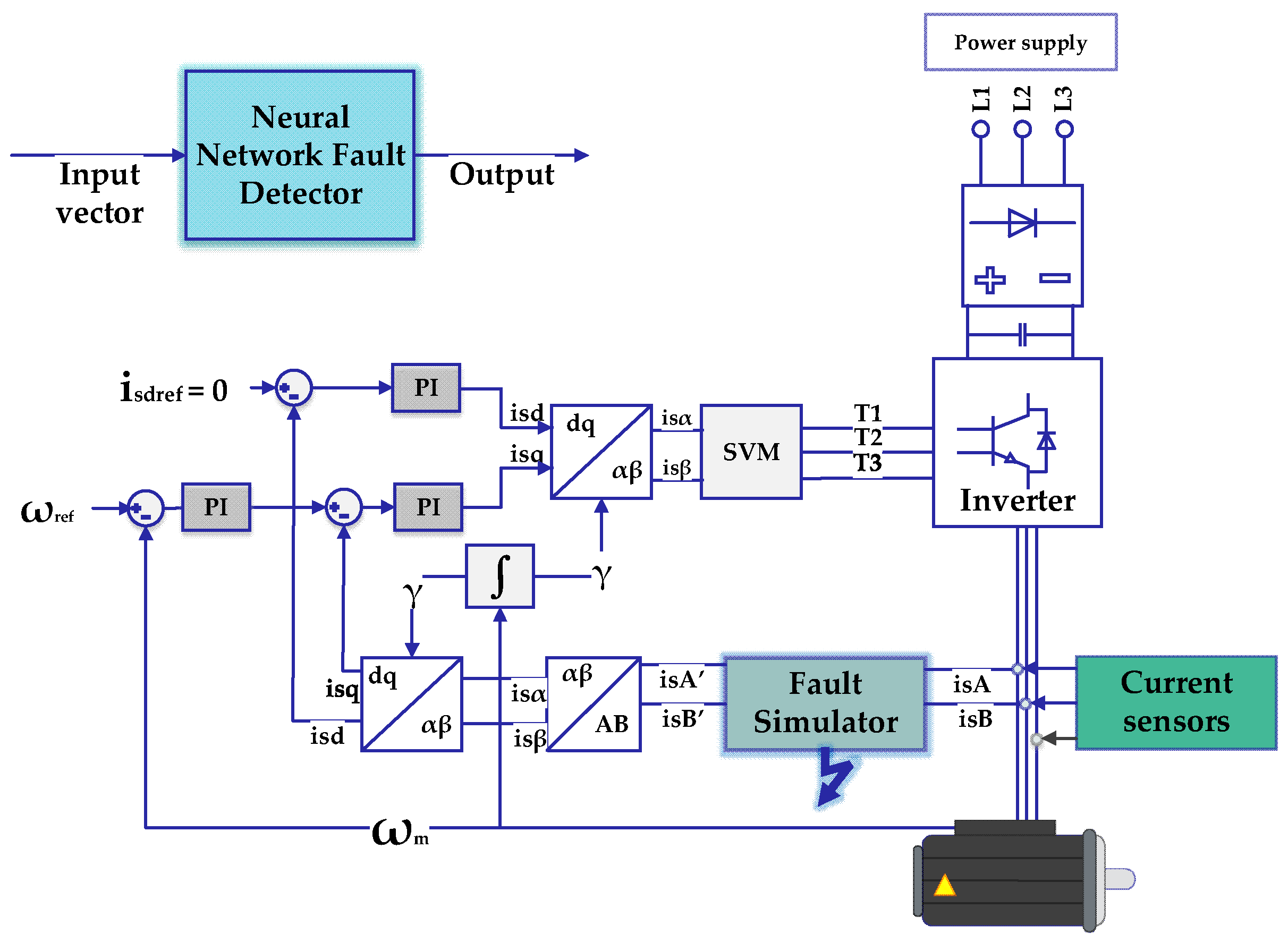
This research paper presents the application of a current sensor fault detection PMSM drive system with the usage of the neural network, presenting simulation results conducted in a Matlab/Simulink environment. A traditional Field-Oriented control was modified with a neural detector of current sensor failure, based on raw signals. Depending on the type of detector, typical current sensor faults were found, including lack of signal, intermittent signal, variable gain, and signal noise in phases A and B. Simulation results are presented for the Multilayer Perceptron for different parameters and various speed conditions. This paper proposes three types of damage detectors. The first detects whether the system becomes corrupted in a 0–1 binary manner. This type detects all common failures. The following types are able to detect fewer types of faults but are able to locate failures. The second type of detector determines which sensor phase failed, while the third additionally detects the type of failure. The application of neural networks in the detection of failures by stator current sensors ensures faster failure detection compared to other methods. This solution also allows us to locate the failure and determine its severity, which is impossible with many simpler methods. Another advantage of the presented solution is the lack of knowledge of the motor model and the fact that raw signals are used. The use of signal analysis methods greatly simplifies the detection process. The neural network was taught with vectors that consist of several dozen to several hundred samples, and each of them accurately indicates damage or its absence. Using raw signals involves training the network with much larger vectors, these are full transients from the structure. Besides, not every sample would show direct damage. This complicates the problem significantly and causes detection errors, especially in dynamic states. However, this approach makes implementations on real-time processors much easier. The developed detector can also be used successfully in an active FTC system. Most of the works describing the use of NN in FTC systems show speed controllers adaptively changing their parameters in the event of external disturbances and minor damage. These are passive systems. There is a gap in the literature discussing the use of neural networks as fault detectors in FTC systems, especially in the case of damages to sensors. The most important goal of the study was to develop a very fast fault detection system for stator current sensors, which would be suitable for electrical drive systems with an increased degree of safety. For this task, artificial neural networks were used, which, according to the authors, are faster than classical algorithmic detection systems and can detect more than one fault type.

This article is organized as follows. In the first Section, FTCS and neural network applications in electric drive systems are discussed. The second Section presents a general diagram of the control structure used in the simulations. A general diagram of the used neural network structure with a description of the damage symptoms used as network inputs, is presented in the third part. The results of the simulations for various neural network structures and testing data based on various speed conditions are presented in Section four. The applicability of the detector in a simple FTC system with a redundant sensor is also discussed in Section four. A short summary of the achieved results is found in the last section.

2. Control Structure of PMSM Drive

The control structure used in the simulations was based on the well-known Field Oriented Control method. The PMSM requires supply from the frequency converter. To ensure high-quality operation, it is necessary to measure the current in at least two phases. The presented control structure uses the measurement from two current sensors to calculate the stator current components. The third sensor is a redundant element. The structure was modified by adding a fault detection block of current sensors based on a neural network. This block will be described in detail in the next part of this paper. The inputs of the neural network are determined in the control structure. The basic diagram of the control structure is presented in Figure 1. All values in the control structure are converted to relative units.

Simulations were carried out for a surface-mounted PMSM with the parameters presented in

Table 1. Parameters of the tested motor.

PN (kW)	Stator Phase Resistance (Ω)	Stator Phase Inductance (mH)	Pp (-)	nN (rpm)	Inertia (kg·m2)	Viscous Damping (N·m·s)	Flux Linkage Established by Magnets (Wb)
2.5	5.56	4.11	2	1500	0.015	100	0.8

Where P_N: nominal motor power, Pp: number of pole pairs, and n_N: nominal speed.

, which were obtained from a real motor. The switching frequency of the modelled inverter in the control structure was 10 khz.

Current sensor faults can be simulated using the appropriate equations, which were implemented in the Fault-Simulator block. These equations are presented in

Table 2. Typical fault types of current sensor.

Type of Fault	Current Value
Variable gain	$i_s^m=(1-\gamma )i_a$
Phase shift	$i_s^m=i_a+i_{offset}$
Signal limit	$i_s^m=i_{sat}$
Noise	$i_s^m=i_a+n(t)$
Lack of signal	$i_s^m=0$
Intermittent signal	$i_s^m=[0,1]$

Where i_s^m: measured current, i_a: real current, n(t): white noise, γ: constant value from the range <−1,1>, i_sat: limited current, ω_offset = 10 Hz phase shift, and A: current amplitude.

[24].

The control structure in healthy conditions ensures the good dynamic properties of the system and stable work. The transient speed for different reference values and the transients of the phase currents, current components, and electromagnetic torque are shown in Figure 2.

3. Structure of the Neural Network Detector

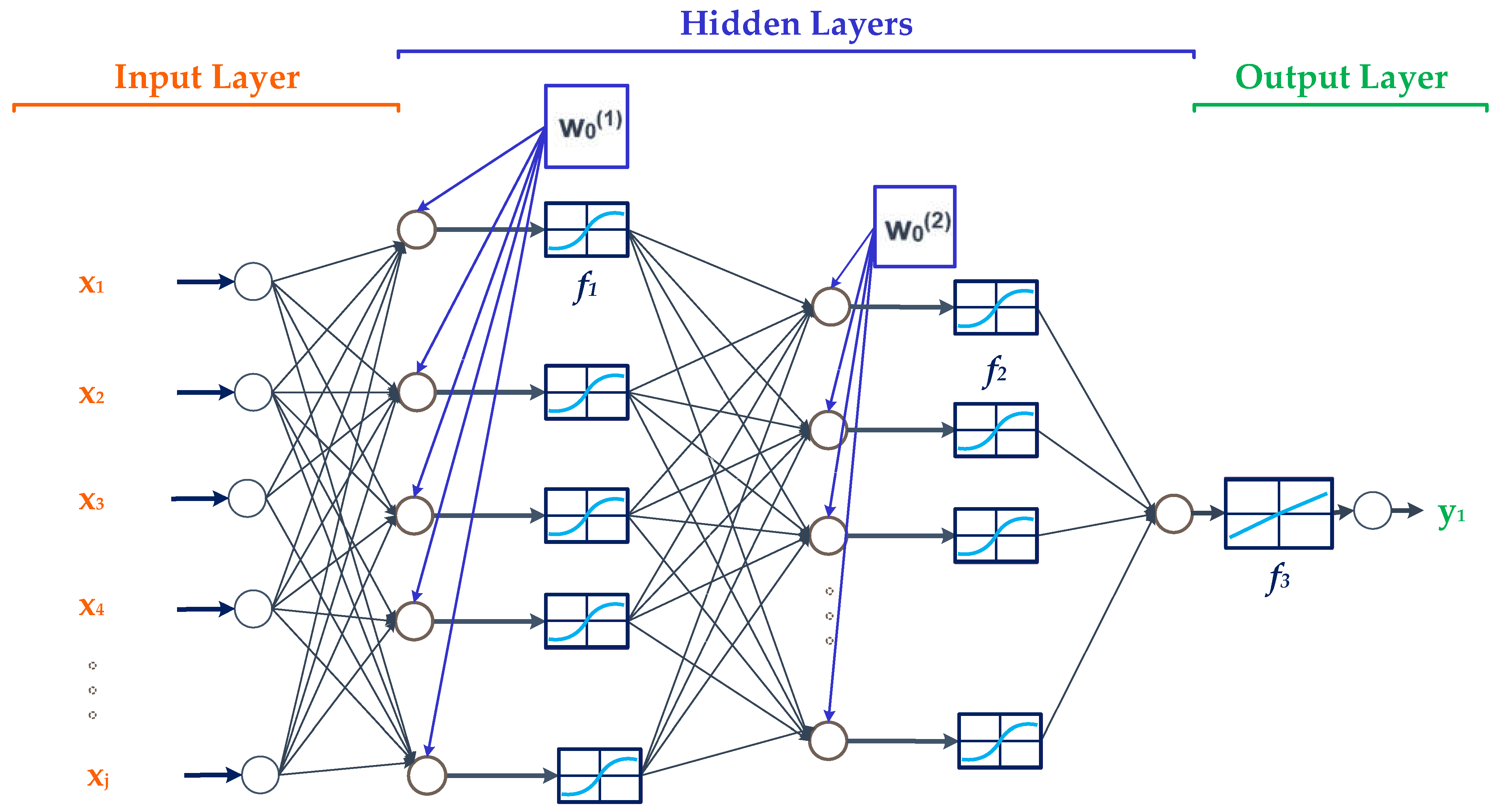
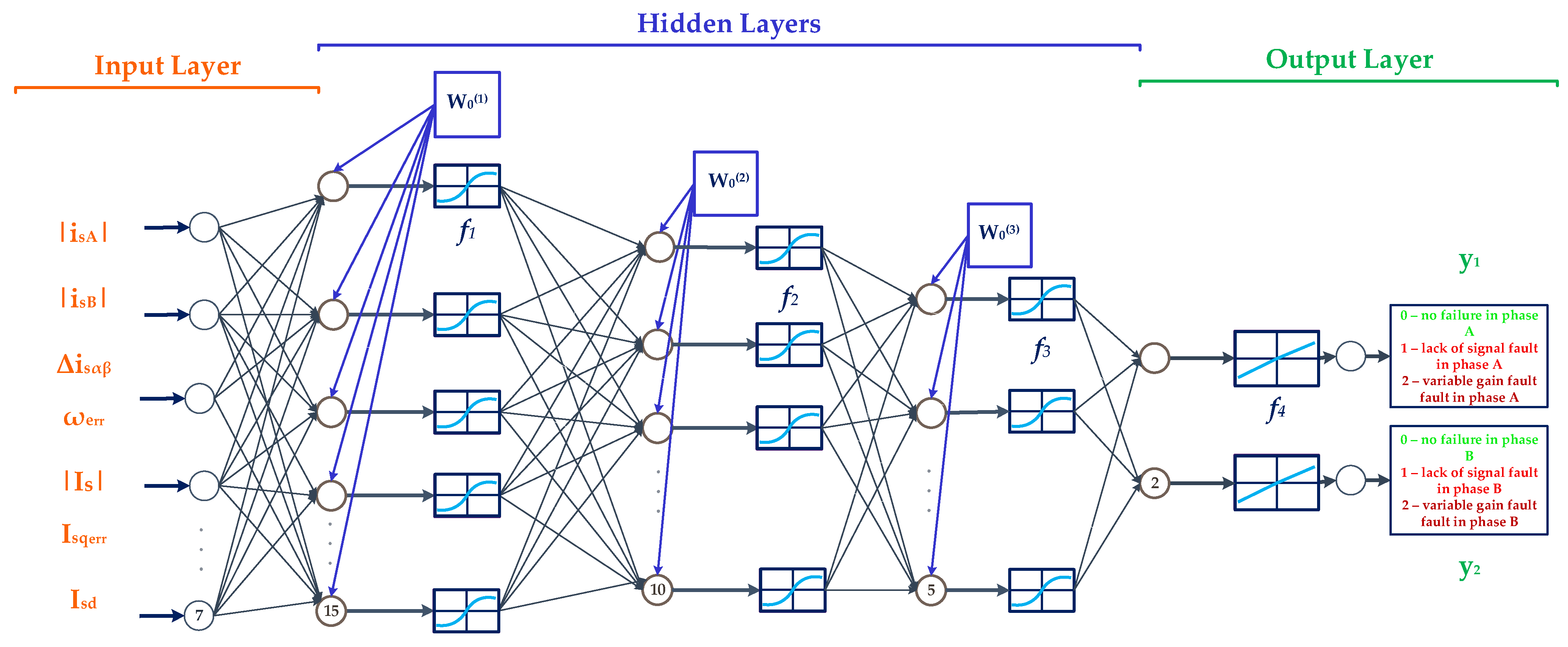
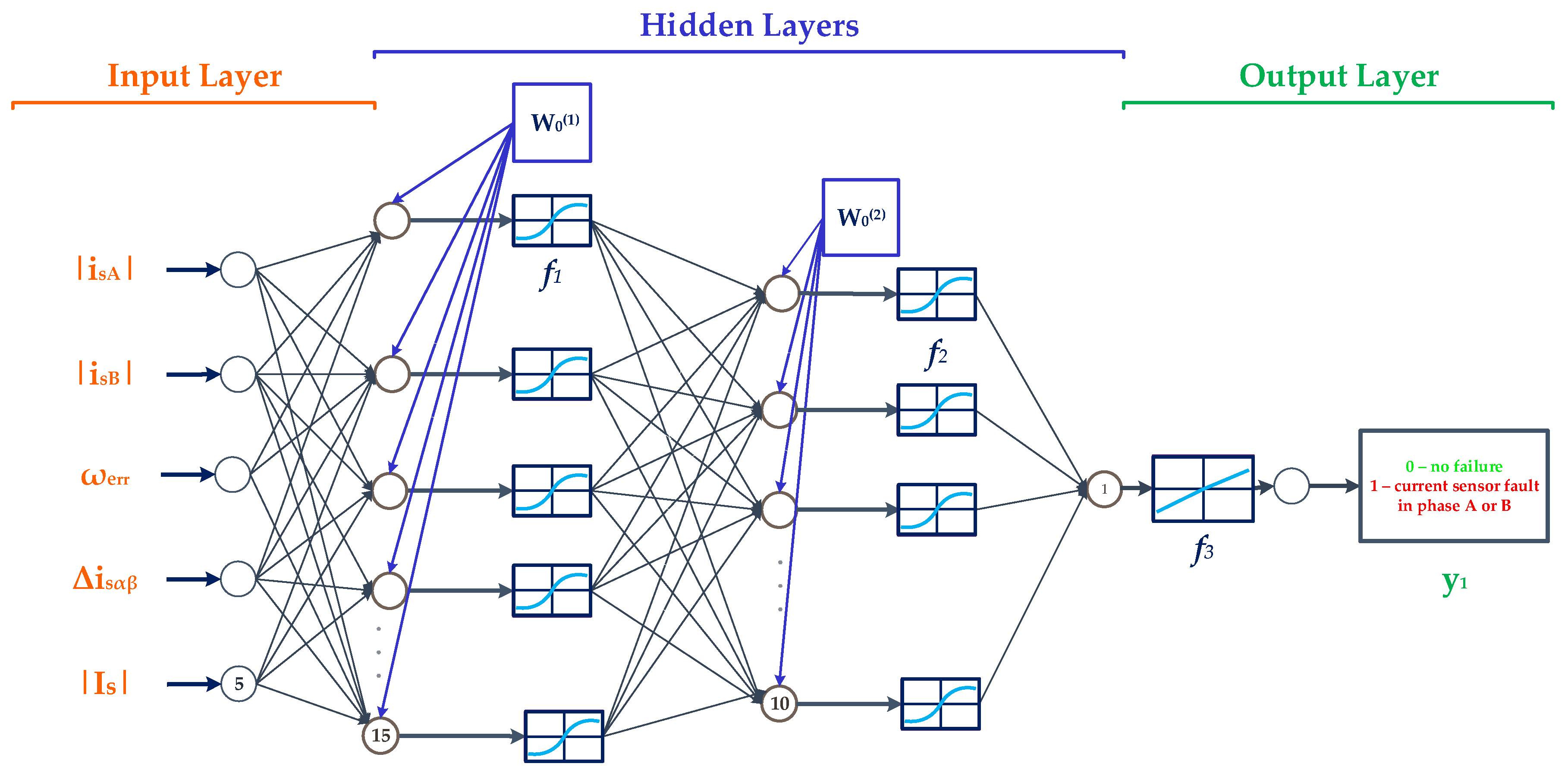
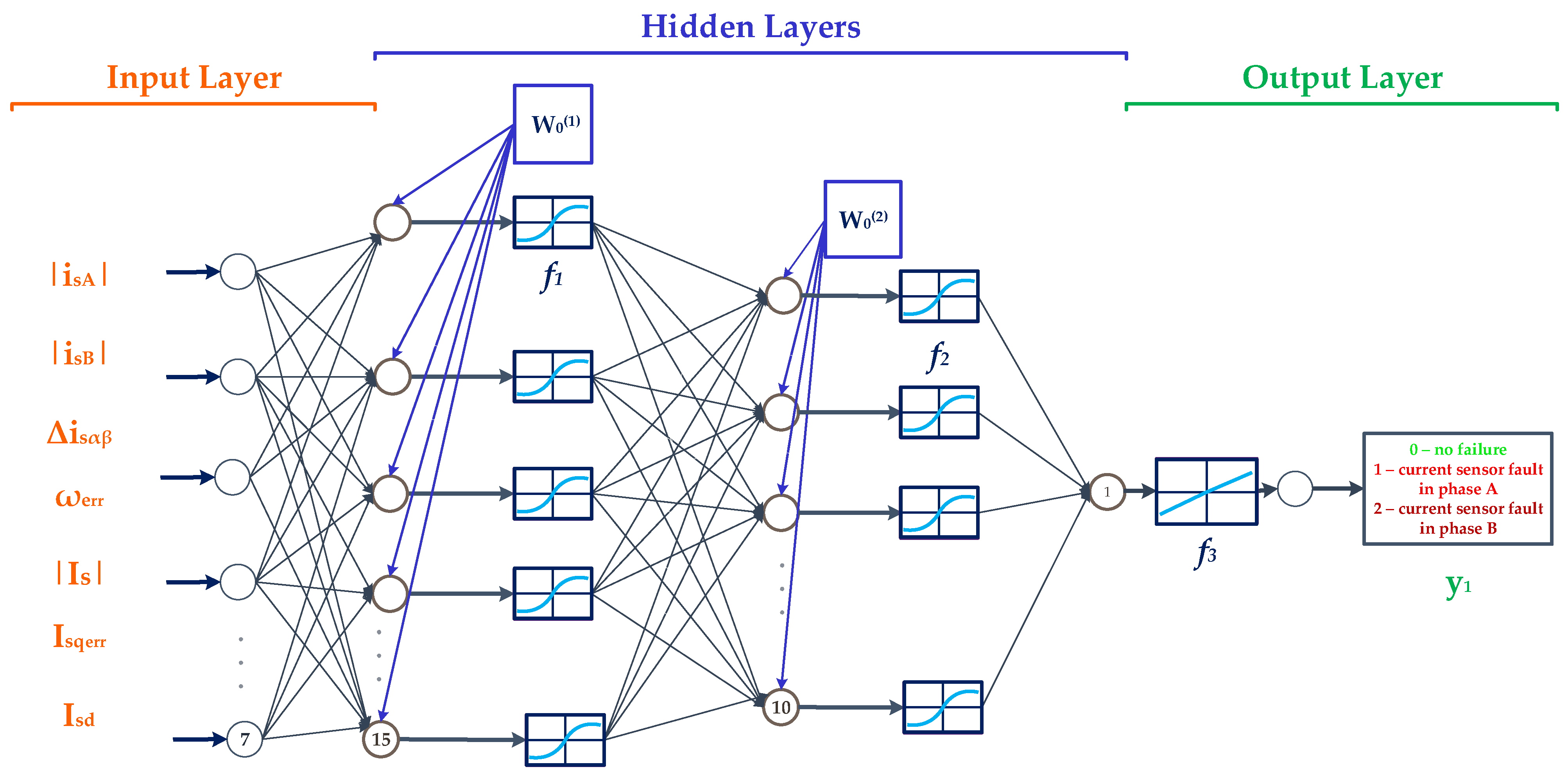
This section presents the neural network detector block structure. Figure 3 shows a general diagram of the neural network structure used in the simulations. Detection is based on a multilayer perceptron. The perceptron is a feedforward neural network consisting of an input layer, n hidden layers, and an output layer. Each neuron in each layer is connected to a neuron of the next layer; there are no connections between the neurons of the same layer.

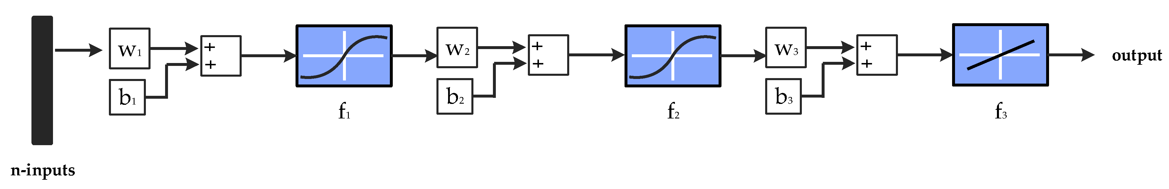
The operation of the perceptron network is based on the following equation [15]:

$$y_k=f_3\left(f_2\left({\displaystyle \sum _{i=1}^M{w}_{ki}^{(2)}\times f_1\left({\displaystyle \sum _{j=1}^N{w}_{ij}^{(1)}\times x_j}+w_0^{(1)}\right)}+w_0^{(2)}\right)\right)$$

(1)

where:

• y_k is the k-th output of the network,
• x_j is the j-th input of the network,
• are the weights of the first and second hidden layers, respectively,
• are the biases in the first and second hidden layers, respectively, and
• f₁, f₂, f₃ are the activation functions.

In this research, the results are presented for three types of detectors. The first one recognizes whether a failure occurred (0–1), the second recognizes a damaged phase, and the third recognizes the type of failure. For each type, tests were carried out for different structures in order to find the optimal number of neurons in the hidden layers. For all tested networks, the Levenberg–Marquardt method with Bayesian regularization was chosen for learning to obtaining better effectiveness. The results were compared using the chosen method and the standard Levenberg–Marquardt method. The standard Levenberg–Marquardt method is very sensitive to the initial values of the weights, which are determined randomly. Adding Bayesian regularization improves the generalization properties of the network. This method aims to minimize the square error of the expected output from that obtained with the smallest possible network weights. It is influenced by the α coefficient, which forces a low weight decay rate. This leads to a reduction in the tendency of the network towards over-fitting to the problem. In the case of the use of the Levenberg–Marquardt method with Bayesian regularization, the objective function takes the form [15,28]:

$$C=\beta E+\alpha E_w$$

(2)

where:

• E is the sum of mean square errors,
• E_w is the sum of squared weights,
• β is the learning factor, and
• α is the decay rate.

The networks were tested with the use of sigmoidal and logistic functions in the hidden layers. The selection of the activation function did not significantly affect the effectiveness of the detection. Therefore, the sigmoidal function was used in the presented version of the detectors. This is the most commonly used function in a multilayer perceptron structure.

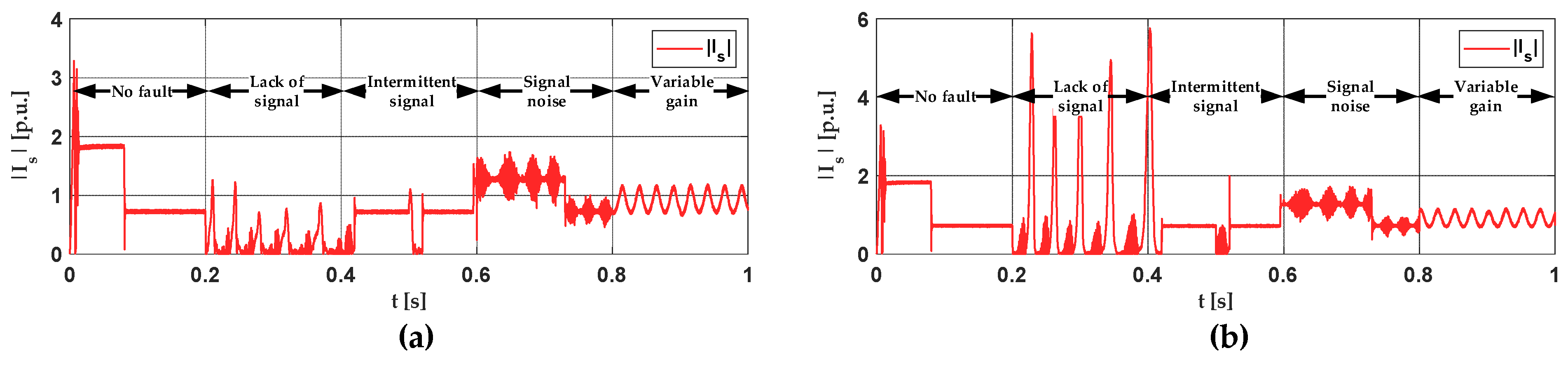
The selection of failure symptoms, which constitute the network’s input signals, was performed empirically. The basic damage symptoms are visible in the modules of the stator current values in phases A and B and in the value of the space vector module |I_s|. The transients of the |I_s| symptom during various failures in phases A and B are shown in Figure 4.

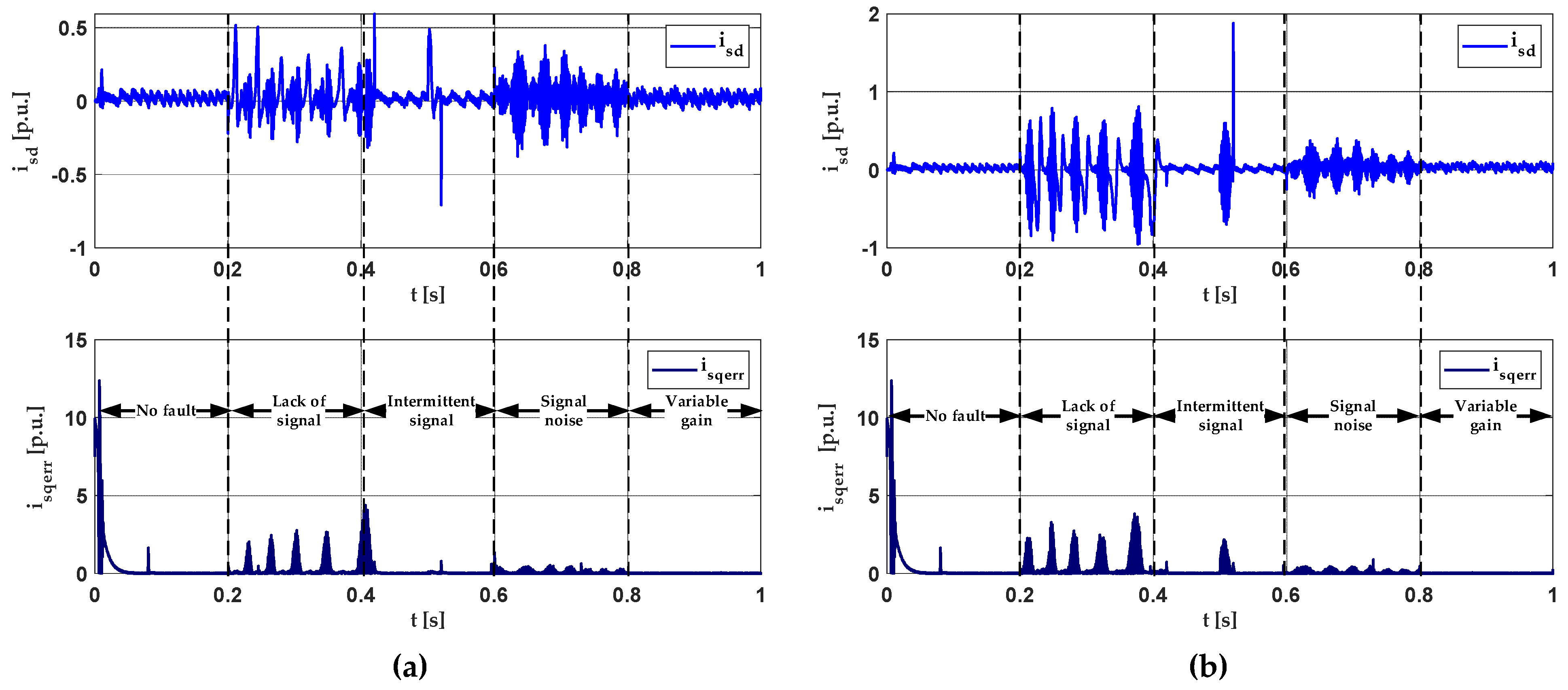
The current, $i_{sq}$, error value and $i_{sd}$ were chosen as symptoms that improved the detection efficiency (Figure 5). As the correct current values depend on the speed, it was decided to use the speed reference and speed error values as an auxiliary symptom.

To significantly improve the detection efficiency of all types of detectors, the fact that the stator current components used in the control structures can be determined using different equations depending on the phases in which the current is measured, was used [11]:

$$i_{s\alpha 1}=\frac{2}{3}(i_{sA}-\frac{1}{2}(i_{sB}+i_{sC})),i_{s\beta 1}=\frac{\sqrt{3}}{3}(i_{sB}-i_{sC})$$

(3)

$$i_{s\alpha 3}=-(i_{sB}+i_{sC}),i_{s\beta 3}=-\frac{\sqrt{3}}{3}(i_{sB}-i_{sC})$$

(4)

$$i_{s\alpha 2}=i_{sA},i_{s\beta 2}=\frac{\sqrt{3}}{3}(i_{sA}+2i_{sB})$$

(5)

where:

• $i_s{}_A$, $i_s{}_B$, are the phase currents, and
• $i_s{}_{\alpha }$, are the stator current components.

The determination of the current components using Equation (3) was based on the measurement of three phases, A, B, C. Equations (4) and (5) are based on measurements in two phases, B, C and A, B, respectively. In a healthy system, these values are equal. After failure appearance, there was a significant difference between them. In the structure, these values were compared. The 0–1 signal was obtained and used as an input of the network.

All the considered input signals for all types of detectors are presented in

Table 3. All considered neural network inputs.

Input	Value
$\left|i_s{}_A\right|$	$\left|i_s{}_A\right|$	$i_s{}_A$—phase A current
$\left|i_s{}_B\right|$	$\left|i_s{}_B\right|$	$i_s{}_B$—phase B current
$\left|I_s\right|$	$|I_s|=\sqrt{i_{s\alpha }{}^2+i_{s\beta }{}^2}$	$i_{s\alpha },i_{s\beta }$—stator current components
$\mathsf{\Delta }{i}_{s\alpha \beta }$ [0, 1]	$i_s{}_{\alpha 1}=i_s{}_{\alpha 2}=i_s{}_{\alpha 3}\wedge i_s{}_{\beta 1}=i_s{}_{\beta 2}=i_s{}_{\beta 3}$	$\mathsf{\Delta }{i}_{s\alpha \beta }$ = [0, 1]
${\omega }_{err}$	${\omega }_{err}=|{\omega }_{ref}-{\omega }_m|$	${\omega }_{ref},{\omega }_m$—reference and measured values of speed
$is{q}_{err}$	$is{q}_{err}=|is{q}_{ref}-isq|$	$is{q}_{ref},isq$—reference and calculated values of stator current component q axis in rotor frame
$i_s{}_d$	$i_s{}_d$	$i_s{}_d$—calculated value of stator current component d axis in rotor frame

.

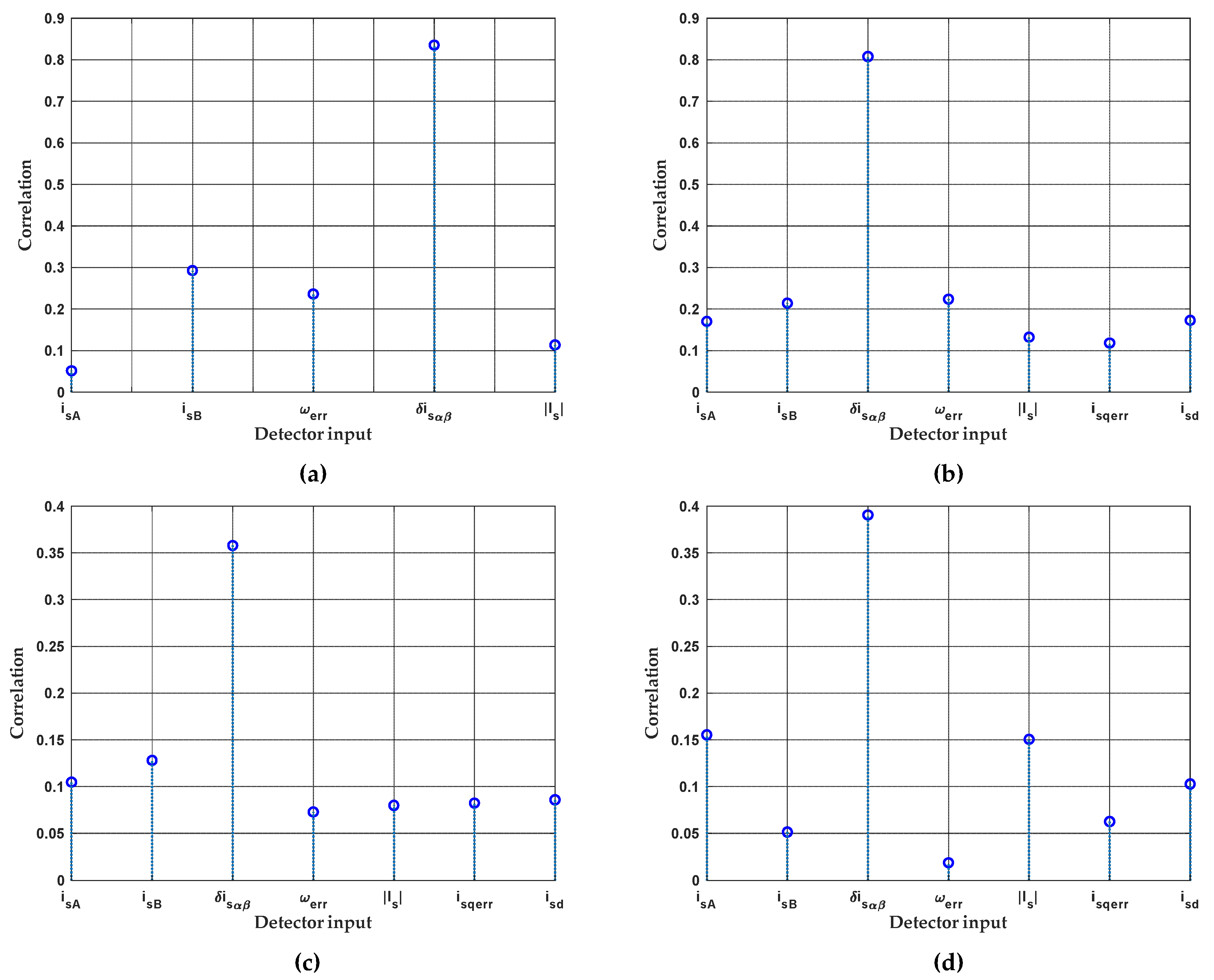
All types of detectors had an extensive input vector. The detection of faults in current sensors using neural networks is a rather complex problem. The input signals take many different values, which are similar in the states of failure and absence. Additionally, the input vectors consist of a huge number of samples. Each of the inputs used improved the effectiveness. The correlation between individual inputs with the detector output is shown in Figure 6. The charts confirmed that the input $\mathsf{\Delta }{i}_{s\alpha \beta }$ significantly improved the detection efficiency and none of the other inputs was irrelevant to the detection process.

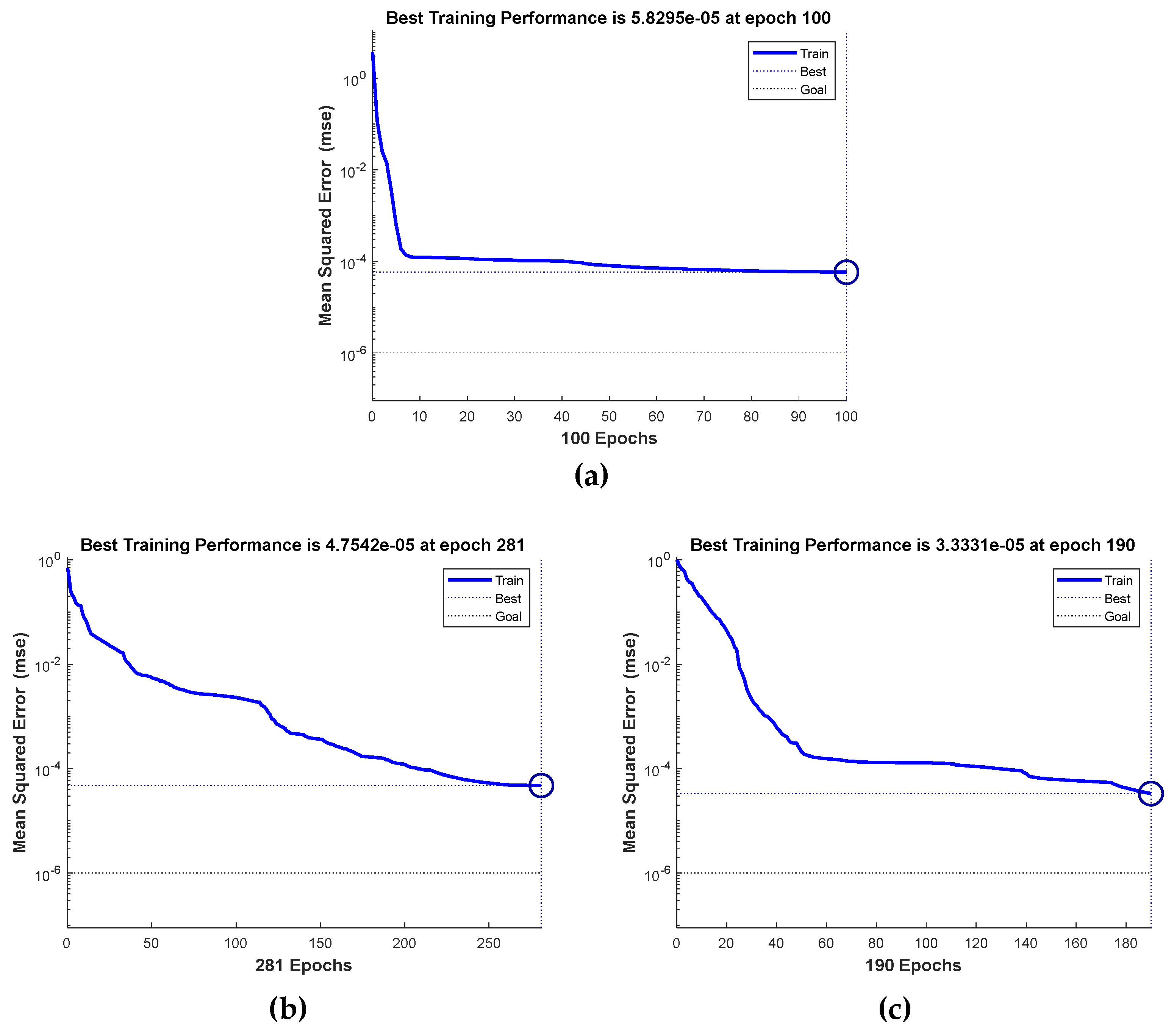
Figure 7 shows the sample mean square learning error transients for all types of detectors. The learning process was interrupted when subsequent iterations minimally reduced the network error.

The neural network training vectors were prepared in the Simulink environment with use of control structure presented in Section 2. Then the learning process was carried out in Matlab. At the last stage, the obtained network parameters were read by a properly prepared block, which allowed for network testing. A diagram of the neural network implemented in the Simulink environment is shown in Figure 8.

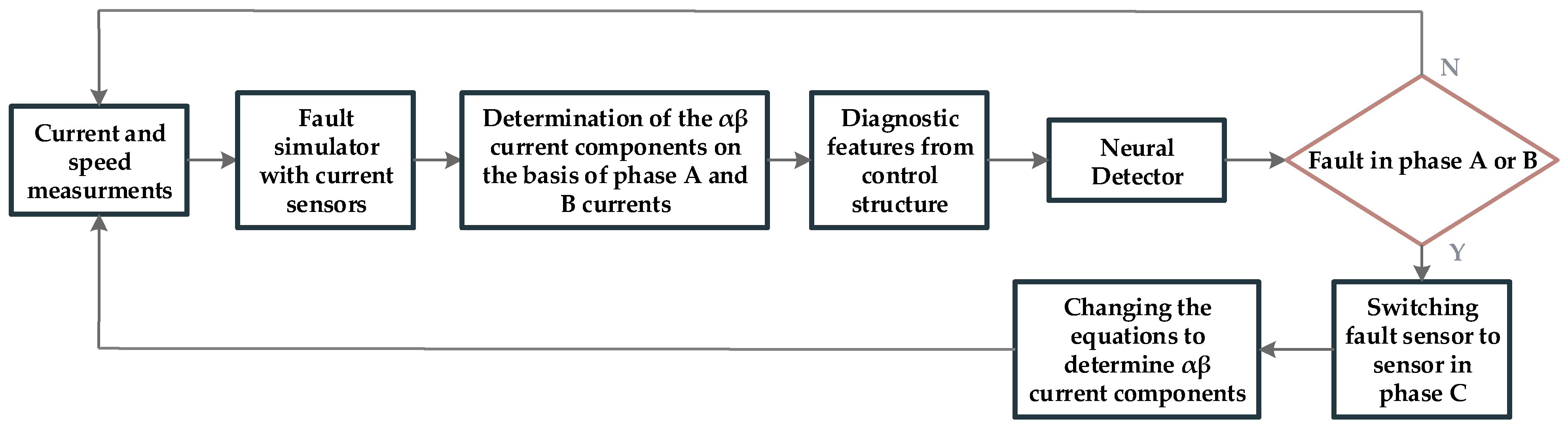
A flow diagram of the complete diagnostic system with fault compensation is presented in Figure 9. The measured currents in phases A and B are transformed in the failure simulator using the equations presented in Table 2. Then the and $i_s{}_{\beta }$ stator current components are determined by the use of the faulty current values which affect the operation of the control structure. At the same time, the necessary input signals are supplied to the NN detector, which determines the state of the current sensors. If a failure is detected, it is compensated by the use of a redundant sensor.

4. Analysis of the Vector-Controlled PMSM Drive with an NN Detector

The point of this article is to present the analysis of a vector-controlled PMSM drive system with the proposed NN detection systems. All results were obtained in Matlab/Simulink software. The model of the control structure was made in the Sim Power System toolbox and the neural network was designed using the Neural Network Toolbox. In this research, the Euler method with a fixed step size equal to 1 × 10⁻⁵ s was used. The Levenberg–Marquardt method with Bayesian regularization was chosen as the network learning method. In the first part of this Section, the effectiveness of the detectors is described. The second part presents a simple FTC system based on the detector described in the first part with a redundant sensor in phase C.

4.1. Fault Detector

Initially, the results are presented for a detector determining 0–1 if a failure was present, i.e., if a lack of signal, intermittent signal, signal noise, and variable gain were detected. In this case, a structure with two hidden layers was employed. One hidden layer turned out to be insufficient. A network with one hidden layer achieved unacceptable effectiveness. The problem turned out to be too complex for such a simple structure. The research was carried out with a different number of neurons in both hidden layers with the same input vector. The best results were obtained for the structure presented in Figure 10 (10-5-1).

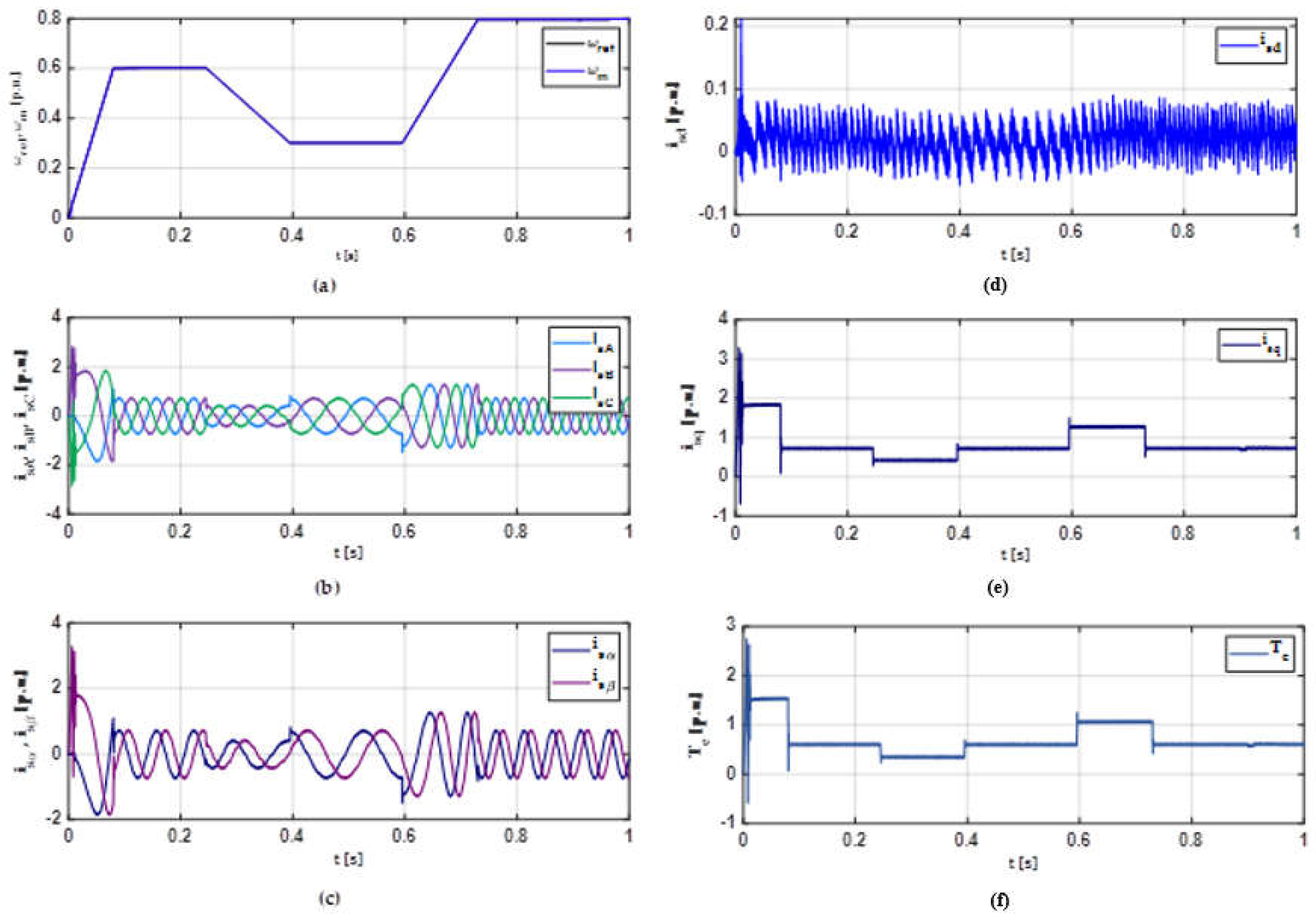
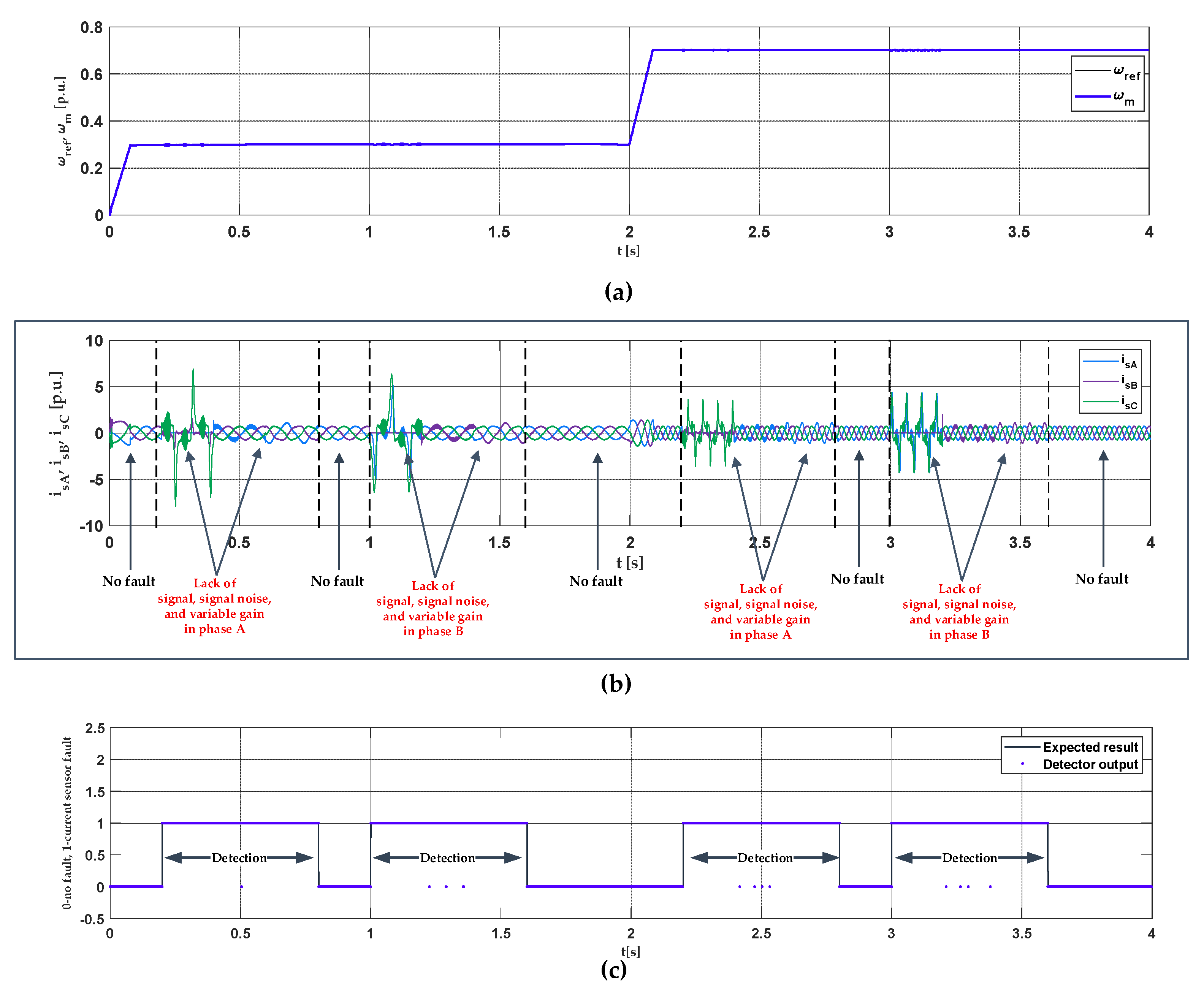
The training vector consisted of samples for two reference speed values (Figure 11). Failures in phase A and B were switched on for each speed. The next types damage switched on were lack of signal, signal noise, and variable gain.

Apart from the detector response to testing data, the transients of the phase currents and the speed are also presented (Figure 12) for some sample values. The detector set correctly output 1 in the event of a failure. The percentage results for all the tested structures are shown in

Table 4. Effectiveness of the first type of detector for different neural network structures.

Structure	15-10-5-1	13-8-3-1	17-12-1	15-10-1	13-8-1	11-6-1	15-1	13-1
Effectiveness	98.2%	98.4%	98.8%	99.1%	98.9%	98.3%	90.9%	85.7%

. The most optimal solution was a network with two hidden layers. One hidden layer was insufficient, while adding a third layer did not significantly affect the effectiveness. The learning process was carried out for two reference speed values (${\omega }_{ref}=0.3$, ${\omega }_{ref}=0.7$) and the tests, which are presented in the percentage results, were performed for five values (${\omega }_{ref}=0.25$, ${\omega }_{ref}=0.4$, ${\omega }_{ref}=0.55$, ${\omega }_{ref}=0.6$, ${\omega }_{ref}=0.75$). In the transient of the testing vector, each of the tested failures was switched on for 0.2 s for each speed in both phases.

One significant advantage of the first type of detector is the fact that it detected a failure when the other detectors in the tested structures produced largely signal noise errors, both in phases A and B. For this type of detector, the signal noise detection also caused the most errors. The detector was characterized by a simple structure (fewer inputs, only two hidden layers, one output), a short learning process, and high effectiveness level for all tested structures, even during dynamic states.

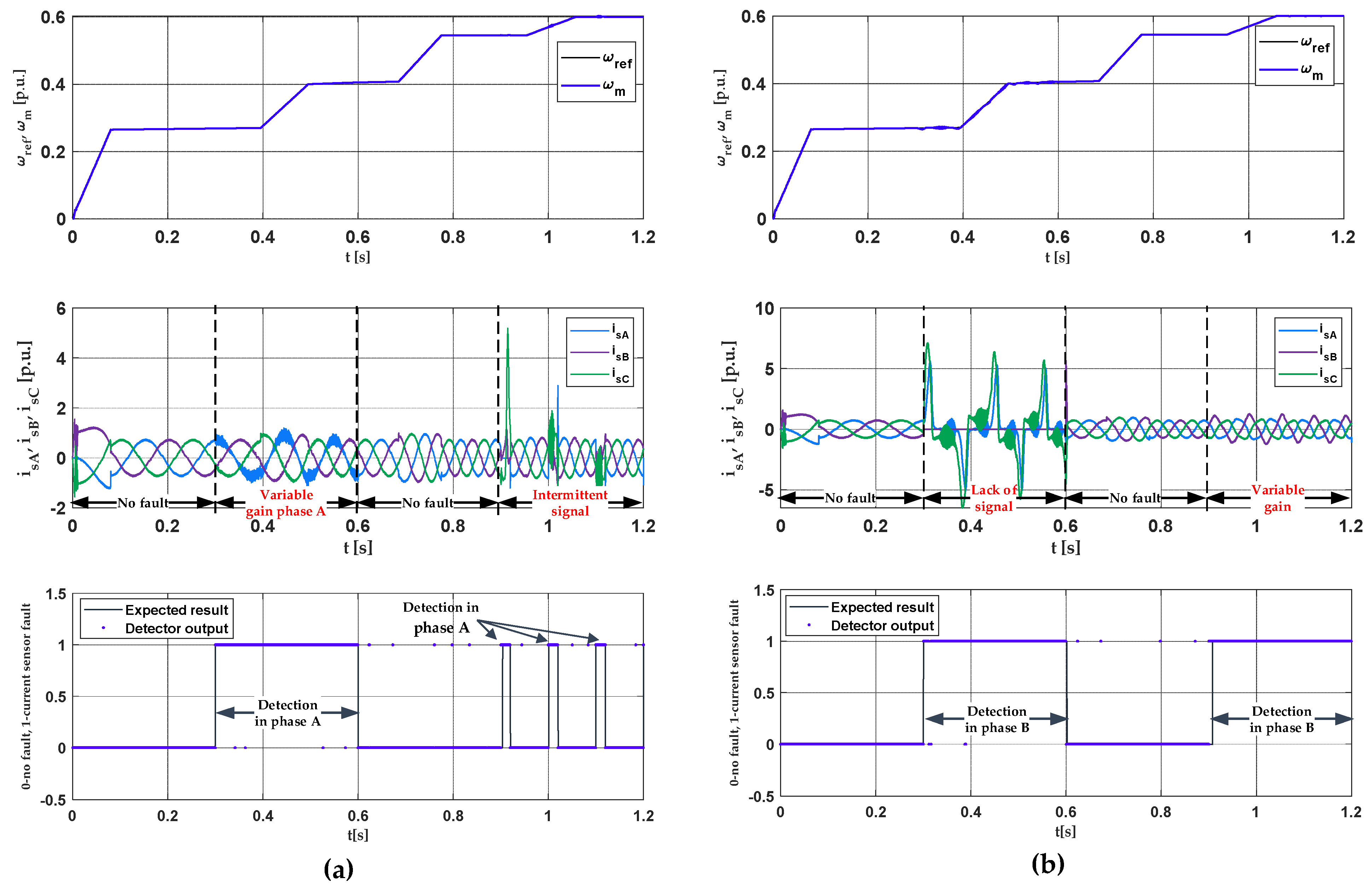
The second type of detector detected lack of signal, intermittent signal, and variable gain, and determined the damage phase. The detector was based on two hidden layers. The research was carried out for a different number of neurons in the hidden layers and different numbers of hidden layers and the same input vector. The most optimal solution was structure 15-10-1 (Figure 13). The reference speed, phase currents, and detector output for this structure for the training data are presented in Figure 14. The structure with three hidden layers differed insignificantly in terms of effectiveness, while the addition of a third hidden layer significantly lengthened the learning process. In this case, the third hidden layer was excessive.

The tests of all structures for the second type of detector were carried out for four values of reference speed (${\omega }_{ref}=0.3$, ${\omega }_{ref}=0.4$, ${\omega }_{ref}=0.5$, ${\omega }_{ref}=0.6$) different from the training values (${\omega }_{ref}=0.35$, ${\omega }_{ref}=0.65$, ${\omega }_{ref}=0.85$), with dynamic states. Sample results for the most effective structure for non-training data are presented in Figure 15. The efficacy results for all tested structures are presented in

Table 5. Effectiveness of the second type of detector for different neural network structures.

Structure	15-10-5-1	13-8-3-1	17-12-1	15-10-1	13-8-1	11-6-1	15-1	13-1
Effectiveness	98.8%	98.6%	97.6%	98.5%	98.0%	97.5%	88.5%	73.6%

. The network was tested by using the vector where all failures were switched on for 0.2 s for all the above specified speeds in both phases.

The optimal structure for the second type of detector was 15-10-1. The use of a larger number of neurons in the hidden layers increased the learning process, but not the efficiency, and the same was true for adding more hidden layers. Fewer neurons led to a decrease in detector efficiency. Too many neurons in the hidden layers caused efficiency to decline. This was because the network was over-fit to the problem. During the network testing process, the structure worked at speeds other than the values used in the learning process, and also in dynamic states. Therefore, it was important that the network retained the appropriate generalization properties. All the investigated structures for the second detector showed a high degree of correct operation, except the networks with one hidden layer. In these cases, the effectiveness was unacceptably low. The detector correctly recognized the damaged phase, despite the influence of the second phase.

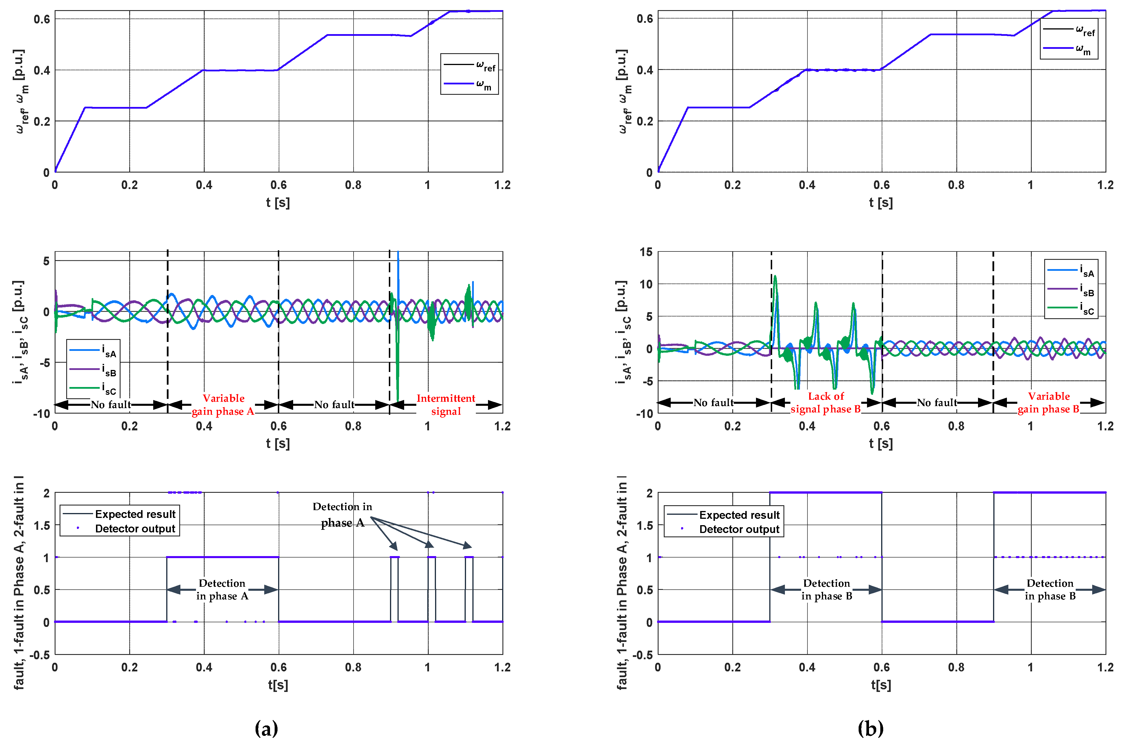
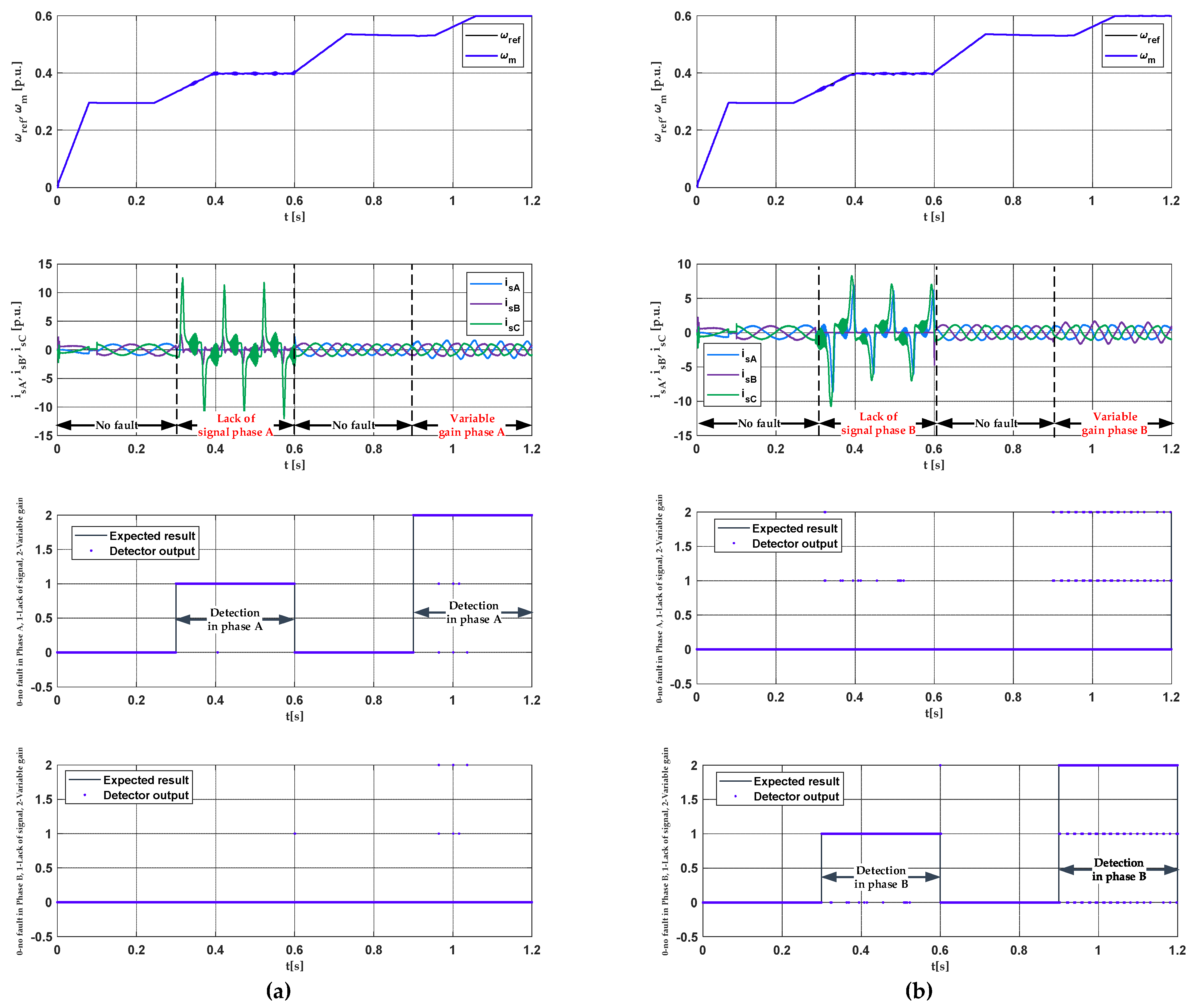
The last type of detector detected the lack of signal, intermittent signal, and variable gain. It also recognized the failure phase and type of fault. The detector response is based on two outputs. The first output specified phase A, where 0 indicated healthy conditions, 1 meant signal interruption, and 2 meant variable gain. The second output defined phase B. In this case, the same training vector was used as for detector type 2, and only the detector output was modified. The detector was based on three hidden layers. A third hidden layer was required to ensure high efficiency. The network with two hidden layers showed too low efficiency, of around 90%. The greatest efficiency was obtained for the structure shown in Figure 16 (15-10-5-2).

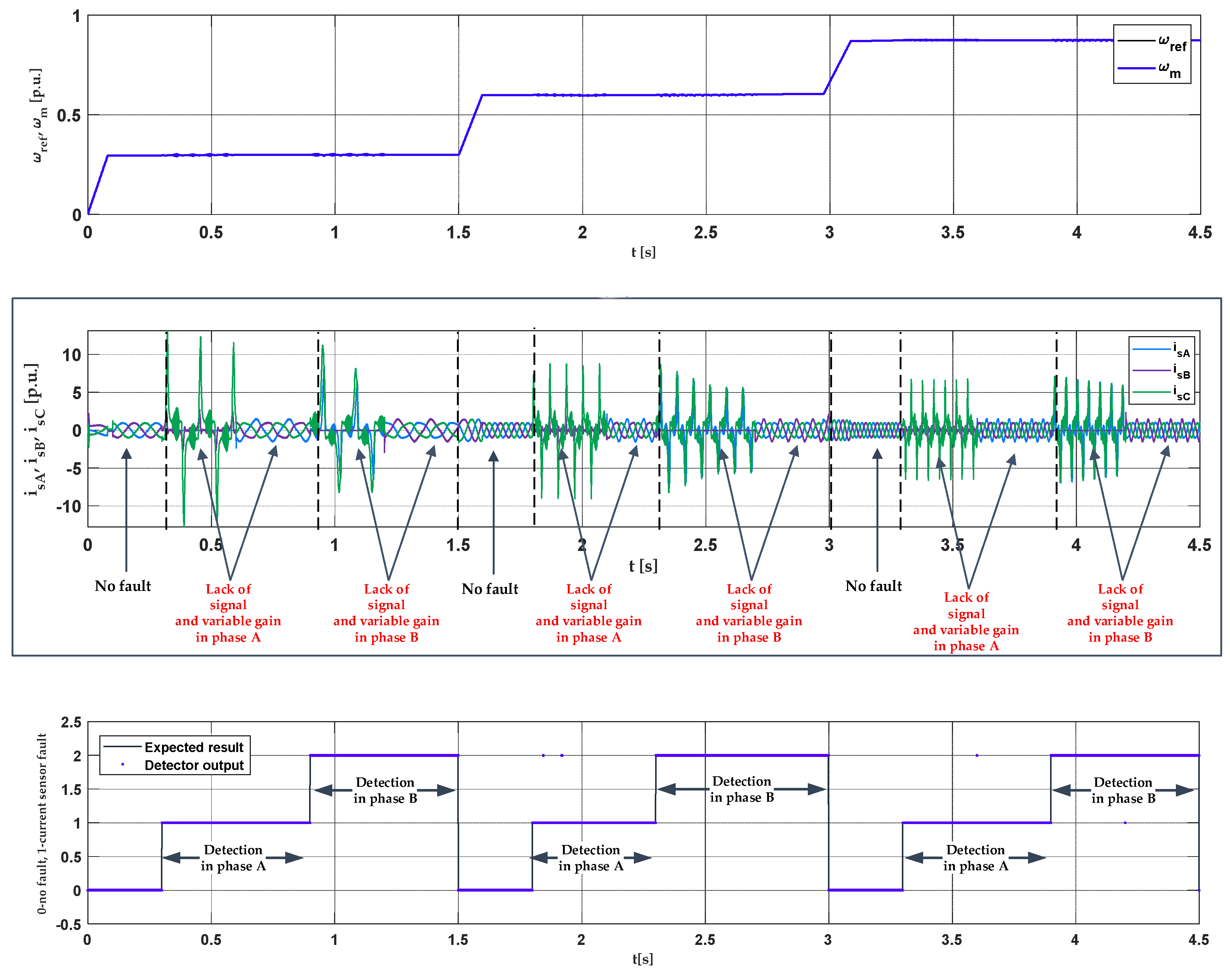
For the structure that obtained the best efficiency, the transients of speed, phase currents, and detector response for the testing data are presented in Figure 17. The percentage results for all tested structures are shown in

Table 6. Effectiveness of the third type of detector for different neural network structures.

Structure	19-14-9-2	17-12-7-2	15-10-5-2	13-8-3-2	15-10-2	13-8-2
Effectiveness output-1	98.4%	98.3%	98.9%	98.5%	91.4%	88.1%
Effectiveness output-2	98.9%	98.3%	98.8%	98.6%	90.8%	87.5%

. The effectiveness tests were conducted for the same training and testing reference speeds as used for the second detector.

In the case of the third type of detector, the efficiency was similar to that of the second type, although the problem was more complex. The use of the third layer allowed for high efficiency. However, at the same time it significantly extended the learning process. This detector not only correctly recognized a damaged phase, but also determined with high efficiency whether it was a failure that significantly affected the control structure. On the basis of the network response figures, it was also observed that the network did not make errors at the level of damage or its absence, but only in phase recognition.

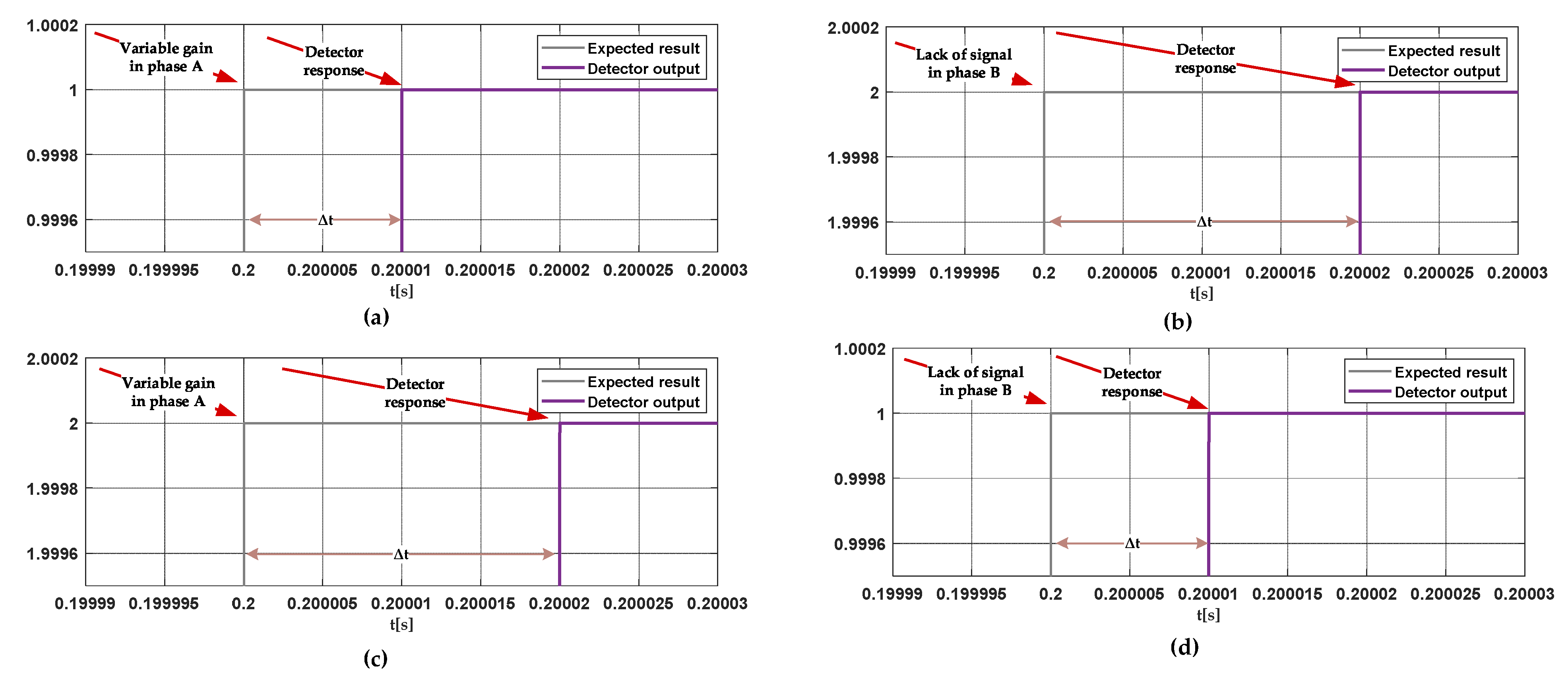
The last important element of the detector operation analysis was the detection time.

Table 7. Detection times for most optimal structures.

Detector	Lack of Signal Phase A	Lack of Signal Phase B	Variable Gain Phase A	Variable Gain Phase B
I type	0.01 ms	0.01 ms	0.01 ms	0.01 ms
II type	0.01 ms	0.02 ms	0.01 ms	0.02 ms
III type	0.01 ms	0.01 ms	0.02 ms	0.02 ms

shows the failure detection times for individual types of detectors. Detection time is also shown in the transient examples (Figure 18).

Detection was almost instantaneous (0.01–0.02 ms), which proves the advantage of the developed solution over many other methods.

4.2. Fault Tolerant System Based on Neural Detector and Redundant Sensor

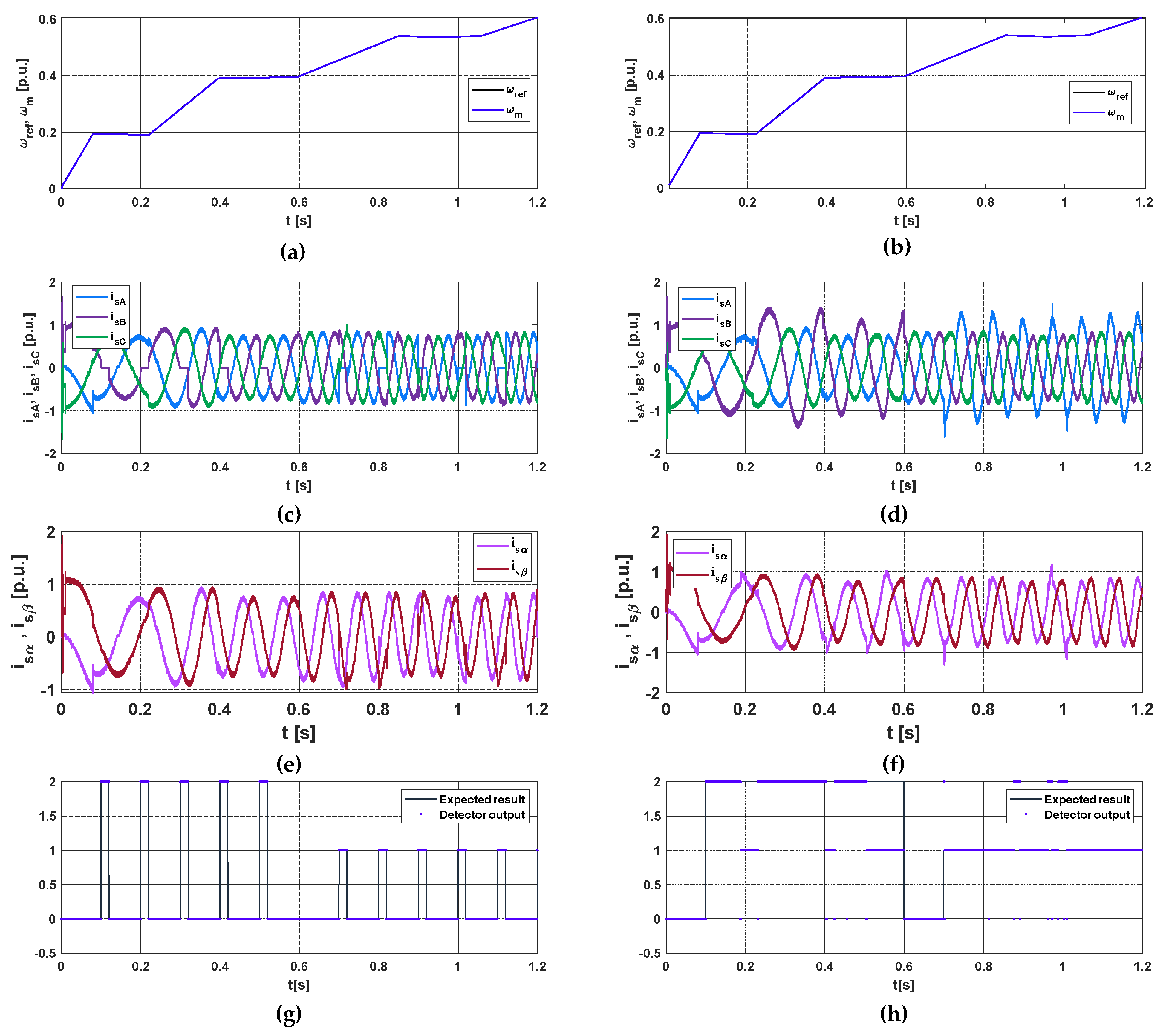
Detector types II and III, due to the possibility of fault location, can be successfully used in the FTC system. The control structure presented in chapter 2 is equipped with three sensors, but in normal operation it uses only two: the in-phase A and B sensors. In the presented FTC system, after information from the detector about the failure and its location are received, the method of determining the $i_s{}_{\alpha }$ and $i_s{}_{\beta }$ of the stator current components was changed. The measurement from the damaged sensor was replaced with the sensor in phase C. The detector response and the basic state variables transients in the FTC system are shown in Figure 19. The results are exemplified by a II-type detector for the 15-10-1 structure.

On the basis of the presented transients, it can be concluded that the proposed method correctly compensates for the influence of damage on the structure in both phases. Despite the disturbances in phase currents, the stator current components αβ were determined correctly and the speed waveforms were not distorted. The network in the FTC structure commits more errors because the signals that indicate the failure reached their pre-failure values e.g., space vector module |I_s|. This was especially visible in the case of the damage with a smaller impact on the variable gain structure. Some distortions appeared in the transients of the stator current components, which resulted from the fact that the sensor had to be switched in the 2nd fault sample. However, this does not interfere with the speed transient and the system can work properly.

5. Conclusions

The paper proposes three types of fault detectors of current sensor faults, based on neural networks, in an electric drive system with PMSM. For all types, the percentage results and diagrams are presented. Although the first type of detector revealed more types of damage, it did not require a more complex structure than the others (two hidden layers, one output). The biggest disadvantage of this solution was that there was no damaged phase detection, which makes compensation impossible. Other types of detectors located the damaged phase, which made it possible to successfully use them in an FTC system with damage compensation, which was the II-type detector presented (Figure 19). Failure localization in a short time of 0.01–0.02 ms (Table 7) gives the application an advantage over many alternative methods. The second type of detector is the most optimal solution. Its learning process was much faster than that of the third type detector due to the less-complicated structure. The location of the damaged phase was sufficient to compensate for it. The type of damage was less-relevant information. The detector determined whether the failure that occurred in the system had a significant impact on its operation and whether immediate compensation was necessary. For this reason, the third type of detector would be used in the most demanding applications. The developed solution can also be transferred to a real drive system. This is supported by the use of raw signals (no need to pre-process measurement data with analytical methods) and the low computational complexity of the learned and implemented neural network on a signal processor. The use of neural networks also allows for faster detection compared to algorithmic methods, which was here proven (Table 7) and allows it to determine the severity of the failure (III type detector). Future work will concern the application of the developed detectors in a more complex FTC structure with fault compensation in simulations and experiments.