Energetic and Financial Optimization of Solar Heat Industry Process with Parabolic Trough Collectors

Abstract

The objective of this work is the investigation of a solar heat industry process with parabolic trough solar collectors. The analysis is conducted for the climate conditions of Athens (Greece) and for five load temperature levels (100 °C, 150 °C, 200 °C, 250 °C, and 300 °C). The examined configuration combines parabolic trough solar collectors coupled to a storage tank and an auxiliary heat source for covering the thermal need of 100 kW. The solar thermal system was optimized using the collecting area and the storage tank volume as the optimization variables. There are three different optimization procedures, using different criteria in every case. More specifically, the solar coverage maximization, the net present value maximization, and the payback period minimization are the goals of the three different optimization procedures. Generally, it is found that the payback period is between five and six years, the net present value is between 500–600 k€, and the solar coverage is close to 60%. For the case of the 200 °C temperature level, the optimum design using the net present value criterion indicates 840 m² of solar collectors coupled to a storage tank of 15.3 m³. The optimization using the solar cover indicates the use of 980 m² of solar collectors with a tank of 28 m³, while the payback period minimization is found for a 560 m² collecting area and an 8-m³ storage tank volume. The results of this work can be used for the proper design of solar heat industry process systems with parabolic trough collectors.

1. Introduction

There are several problems in the domain of energy, which are mainly associated with fossil fuel depletion [1], increasing energy demand [2] and global warming [3]. The industrial sector is a high energy-consuming sector with around 50% of the worldwide energy consumption [4]. The majority of the energy consumption in the industries is for the heat process; this percentage reaches up to 70% [5]. The usual way for obtaining the demanded heat is by using fossil fuels [6], which has negative environmental impacts, as well a high operational cost.

The use of solar energy for covering totally or partially the heat process demand of the industries is not a novel idea, but it is revisited [7,8] due to the serious environmental problems, as well as the fossil fuel depletion in the future [9,10,11]. The processes in the industries cover a great range of low, medium, and high temperatures [12,13]. Below, usual industries with the respective typical temperature ranges for the demanded heat are given [7,8]:

• Dairy: 60–180 °C
• Food: 60–120 °C
• Paper: 60–120 °C
• Chemical: 60–260 °C
• Bricks and plastics: 60–220 °C
• Automobile: 50–120 °C
• Agriculture: 80–90 °C
• Metal: 160–180 °C

It is essential to state that every industry may need heat for more than one process. For instance, the dairy industry needs process heat for pressurization at 60–80 °C, sterilization at 100–120 °C, and drying at 120–180 °C [7].

The parabolic trough solar collector (PTC) is the most mature solar concentrating technology [14,15] that is able to cover all of the previously presented temperature levels for the heat process in the industries [7]. The PTC can efficiently produce useful heat for temperatures up to 400 °C with thermal oil as a working fluid, and up to 550 °C with molten salts [15]. So, the use of PTC is a promising choice in the solar heat for an industrial process (SHIP). Moreover, other kinds of solar collectors are the flat plate collectors (FPC) for temperatures up to 100 °C, the evacuated tube collector (ETC) for temperatures up to 150 °C, and the linear Fresnel reflector (LFR) up to 300 °C [16].

In the literature, there are various studies for SHIP in various locations over the world.

Table 1. Summary of solar heat industrial process studies. PTC: parabolic trough solar collector, FPC: flat plate collectors, LFR: linear Fresnel reflector.

Study	Country	Application or Industry	Collector Type	T	Aa	V	f	Q
				(°C)	(m2)	(m3)	(%)	(MW)
Kalogirou [17]	Cyprus	Hot water	PTC	85	300	25	50	-
Guerro and Quijano [18]	Spain	Cork	PTC	100	432	15	65	0.26
Abdel-Dayem [19]	Egypt	Steam	PTC	175	1958	-	10	-
Pietruschka et al. [20]	Austria	Food	FPC	95	1200	-	-	0.65
	Italy	Bricks	LFR	180	2640	-	-	1.5
	Spain	Dairy	PTC	185	2040	-	-	1.0
Silva et al. [21]	Spain	Heat	PTC	150	1000	100	67	0.1
Vittoriosi et al. [22]	Italy	Bricks	LFR	260	2700	-	20	1.2
El Ghazzani et al. [23]	Marocco	Hot air	PTC	160	39,760	3300	57	10.5
Tian et al. [24]	Denmark	District heating	FPC	75	5960	2430	-	-
			PTC	95	4039

summarizes all of the investigated studies. In 2001, Kalogirou [17] theoretically examined a solar system with PTC for hot water production at 85 °C for Cyprus. He found the optimum collecting area to be 300 m² and the optimum storage tank for this collecting area at 25 m³. The solar coverage for this energetically optimized system was around 50% for Spain. Guerro and Quijano [18] studied the use of PTC for heat production at 100 °C for a cork industry. Their system has a nominal capacity of 260 kW with a 432 m² collecting area and 15 m³, while the solar coverage was 65%. Abdel-Dayem [19] investigated a steam production system with PTC for Egypt. The system includes 1958 m², that cover a load of 175 °C in a 10% percentage.

Pietruschka et al. [20] examined the use of different systems in different locations. Firstly, they investigated a system with FPC for a food industry in Austria. This system produces heat at 95 °C and includes 1200 m² of collectors that cover a load of 650 kW. The second system includes LFR for a brick industry in Italy. This system produces heat at 180 °C and includes 2640 m² of collectors that cover a load of 1.5 MW. The last system includes a PTC for a dairy in Spain. This system produces heat at 180 °C and includes 2040 m² of collectors that cover a load of 1.0 MW.

Silva et al. [21] studied a heat production system at 150 °C with PTC in Spain. The nominal heat production was 100 kW that is covered in a percentage of 67% with a 1000 m² collecting area and 100 m³ of storage tank volume. Vittoriosi et al. [22] studied the use of LFR in a 1.2-MW installation in Italy. They found that the total system coverage was 20% with 2700 m² of collectors for heat production at 260 °C. El Ghazzani et al. [23] found that the use of 39,760 m² of PTCs with a storage tank of 3300 m³ were able to cover 57% of a 10.5-MW load at 160 °C in Morocco.

Recently, in 2018, the combination of PTCs and FPCs was recently examined by Tian et al. [24] for Denmark. They used 5960 m² of FPCs for heat production at 75 °C, and 4039 m² of PTCs for heat production at 75 °C. There is also a storage volume of 2430 m³. The load of the districting heating was covered by both collector types, with the FPC producing a bit lower than 5 kWh/m², and the PTC producing a bit more than 5 kWh/m².

The previous literature review indicates that the use of PTC for producing heating for industrial processes or other heat applications is a promising choice. Various systems have been studied worldwide, especially in locations with relatively high solar potential. Greece is a country with high solar potential, which ranges from 1400 kWh/m² up to 1800 kWh/m² yearly. Athens is the largest city in Greece; it is located approximately in the middle of Greece (about 38° latitude), and it is a representative location for investigation with about 1600 kWh/m² solar potential [25].

The objective of this work is to design an optimum industrial process heat system for the climate conditions of Athens (Greece). This system includes PTCs and an auxiliary system for covering the heating load during the period without solar irradiation. This system has a nominal load demand of 100 kW, and it is investigated theoretically for temperature levels between 100–300 °C with a 50 °C step. This work is a theoretical approach for a solar-assisted industrial heat process, and the results can be applied in different industrial processes. This system is studied energetically and financially for different design scenarios. More specifically, different combinations of solar collecting areas and storage tank volumes are tested for all the years and periods. The system is optimized with three different criteria: the maximization of the solar coverage, the maximization of the net present value (NPV), and the minimization of the payback period (PP) of the investment. The results of this work clearly show the coverage of a solar system with PTC for heat process, as well as its financial sustainability. Moreover, the optimum system size is variable with the different optimization goals, which is discussed in this work. The innovation of this paper is based on the investigation of the present system in Greece, as well as the optimization with different criteria. The comparison of the optimization with energy and financial criteria separately is something that is not found in the present literature, and so this work has to add something new to this domain. The final conclusions of this work can clearly prove if the use of PTCs for heating production is a promising choice for Greece, and whether they can be utilized by various researchers and engineers. Finally, it has to be said that the innovation of this work is mainly associated with the investigation of a solar heat industrial process system in Greek climate conditions, as well as the optimization of the system with different criteria.

2. Material and Methods

2.1. The Examined System-General Description

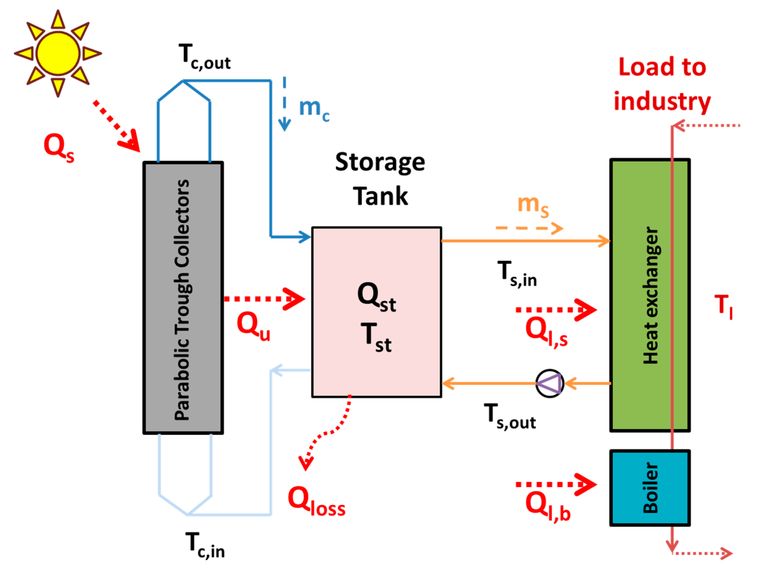
Figure 1 depicts the examined configuration with the proper details. Parabolic trough solar collectors are used in order for the solar irradiation to be converted into useful heat. Thermal oil flows in the PTC field, and it is stored in the storage tank. The thermal oil from the tank feeds the heat exchanger, while there is a boiler in order for the proper heat amount to be given in the load. More specifically, the examined solar field is assumed to have the modules to parallel connection. So, all of the pipes from the PTC outlets are connected, and they are delivered in the upper part of the tank, which is the hot tank region. Cold oil from the tank bottom leaves the tank, and it is separated in different smaller pipes that feed the various modules. In the other side of the tank, hot thermal oil leaves the tank, and it goes to the heat exchanger in order to put heat into the load. The colder oil from the heat exchanger outlet returns to the storage tank bottom region.

In the present work, for a specific combination of collecting area and storage tank volume, the inputs in the system are the solar direct beam irradiation (G_b), the ambient temperature (T_am), and the load temperature (T_l). The developed program, which is presented in the following subsections, calculates the other parameters as the inlet fluid temperature in the solar field (T_c,in), the outlet fluid temperature for the solar field (T_c,out), the fluid inlet temperature in the heat exchanger (T_s,in), the outlet temperature of the heat exchanger (T_s,out), as well as the various heat rates (Q).

2.2. The Solar Field

The Eurotrough module is used in this work, which is a PTC with an evacuated tube receiver [26,27,28]. This module has a collecting area of 70 m² and various modules in parallel connection from three up to 14 have been investigated. The working fluid is Therminol VP-1 [29], and the mass flow rate in every module is selected at 4 kg/s [30]. Moreover, it is important to state that the collectors are located in a north–south direction, and they track the sun in the east–west direction.

Table 2. Basic data about the solar collector [26,27,28].

Parameter	Symbol	Value
Module area	Amod	70 m2
Number of solar modules	Nmod	3 to 14 modules
Flow rate	mc	4∙Nmod (kg/s)
Module length	L	12 m
Receiver diameter	Dr	70 mm
Concentration ratio	C	26.2

includes the main data about the examined module.

The solar irradiation in the collector aperture (Q_s) is calculated as:

$$Q_s=A_a\cdot G_b$$

(1)

where the total collecting area (A_a) is given as:

$$A_a=N_{mod}\cdot A_{mod}$$

(2)

The thermal efficiency of the solar collector (η_th) is defined as:

$${\eta }_{th}=\frac{Q_u}{Q_s}$$

(3)

The useful heat production (Q_u) is calculated as:

$$Q_u=m\cdot c_p\cdot \left(T_{out}-T_{in}\right)$$

(4)

The thermal efficiency (η_th) can be estimated using the following literature formula for the Eurotrough model [30]:

$${\eta }_{th}=0.7408\cdot K\left(\theta \right)-0.0432\cdot \frac{T_{c,in}-T_{am} }{G_b}-0.000503\cdot \frac{{\left(T_{c,in}-T_{am}\right)}^2 }{G_b}$$

(5)

The incident angle modifier (K) is calculated for this collector, according to the literature [31], as below with the solar angle (θ) in degrees:

$$K\left(\theta \right)=\cos \left(\theta \right)-5.25091\cdot {10}^{-4}\cdot \theta -2.859621\cdot {10}^{-5}\cdot {\theta }^2$$

(6)

The present tracking system makes the PTC follow the sun in the east–west direction, while the PTC axis is in the north–south direction. In this case, the incident angle (θ) is calculated as below [30,32]:

$$\cos \left(\theta \right)=\sqrt{{\cos }^2\left({\theta }_z\right)+{\cos }^2\left(\delta \right)\cdot {\sin }^2\left(\phi \right)}$$

(7)

More details about the calculation of the solar angles can be found in [30,32].

2.3. Storage Tank

The storage tank is assumed to be a cylindrical insulated tank with a thermal loss coefficient equal to 0.8 W/m²K. The storage tank is an open tank without heat exchangers that is modeled with five thermal zones, and all of the zones have the same thickness in every case. More details about this modeling can be found in [30,32,33]. The diameter of the tank is assumed to be the same as its length [30]. This assumption has been checked with a simple sensitivity analysis, and it is found that it has no practical impact on the results. Moreover, it is assumed that the stream temperature to the load (T_s,in) is the temperature in the upper zone, while the temperature to the solar field (T_c,in) is equal to the temperature of the last node. The general energy balance in the storage tank is given below:

$$Q_{st}=Q_u-Q_{loss}-Q_{l,s}$$

(8)

The stored energy (Q_st) is the difference between the heat input from the solar field (Q_u) and the heat output to the load (Q_l,s), and the thermal losses to the ambient of the tank (Q_loss). The stored energy can be expressed as:

$$Q_{st}=\rho \cdot c_p\cdot V\cdot \frac{d{T}_{st}}{dt}$$

(9)

The volume of the storage tank (V) is a parameter of this work, and it is investigated for a great range in order to determine its optimum value. More details will be given in the following sections.

2.4. Load Heat Exchanger

The load heat exchanger is used in order for the heat to be transfered from the load to the industrial stream. In this work, the industrial stream is assumed to have a constant temperature (T_l) that is examined parametrically from 100 °C up to 300 °C, with a step of 50 °C. The energy balance in the heat exchanger is given below:

$$Q_{l,s}=m_s\cdot c_p\cdot \left(T_{s,in}-T_{s,out }\right)$$

(10)

The heat exchanger effectiveness (η_hex) was selected at 70%, and it is defined as:

$${\eta }_{hex}=\frac{T_{s,in}-T_{s,out}}{T_{s,in}-T_l}$$

(11)

The mass flow rate in every case is selected to be the one that gives the maximum load (Q_l), which is 100 kW for this case. Generally, the minimum pinch difference in the heat exchanger was about ~5 K in all of the cases. The pressure level in the thermal oil circuit is selected to be at 15 bar in order to keep the oil in its liquid phase. Moreover, it has to be said that in every case, the thermal oil has temperature levels similar to the load temperature, and there are not extremely high deviations between them, because this would increase the exergy destruction losses of the system.

2.5. System Operation

The system is assumed to operate about 350 days per year, or 8400 h per year. The heat demand is 100 kW, which is covered from the solar energy or the boiler.

The energy parameters (E) can be calculated by integrations of the energy rates (Q) for the entire year:

$$E=\underset{t=0 \mathrm{h}}{\overset{t=8760 \mathrm{h}}{{\displaystyle \int }}}Q dt$$

(12)

The solar cover (f) is a critical parameter, and it is defined as:

$$f=\frac{E_{l,s}}{E_l}$$

(13)

2.6. Weather Data

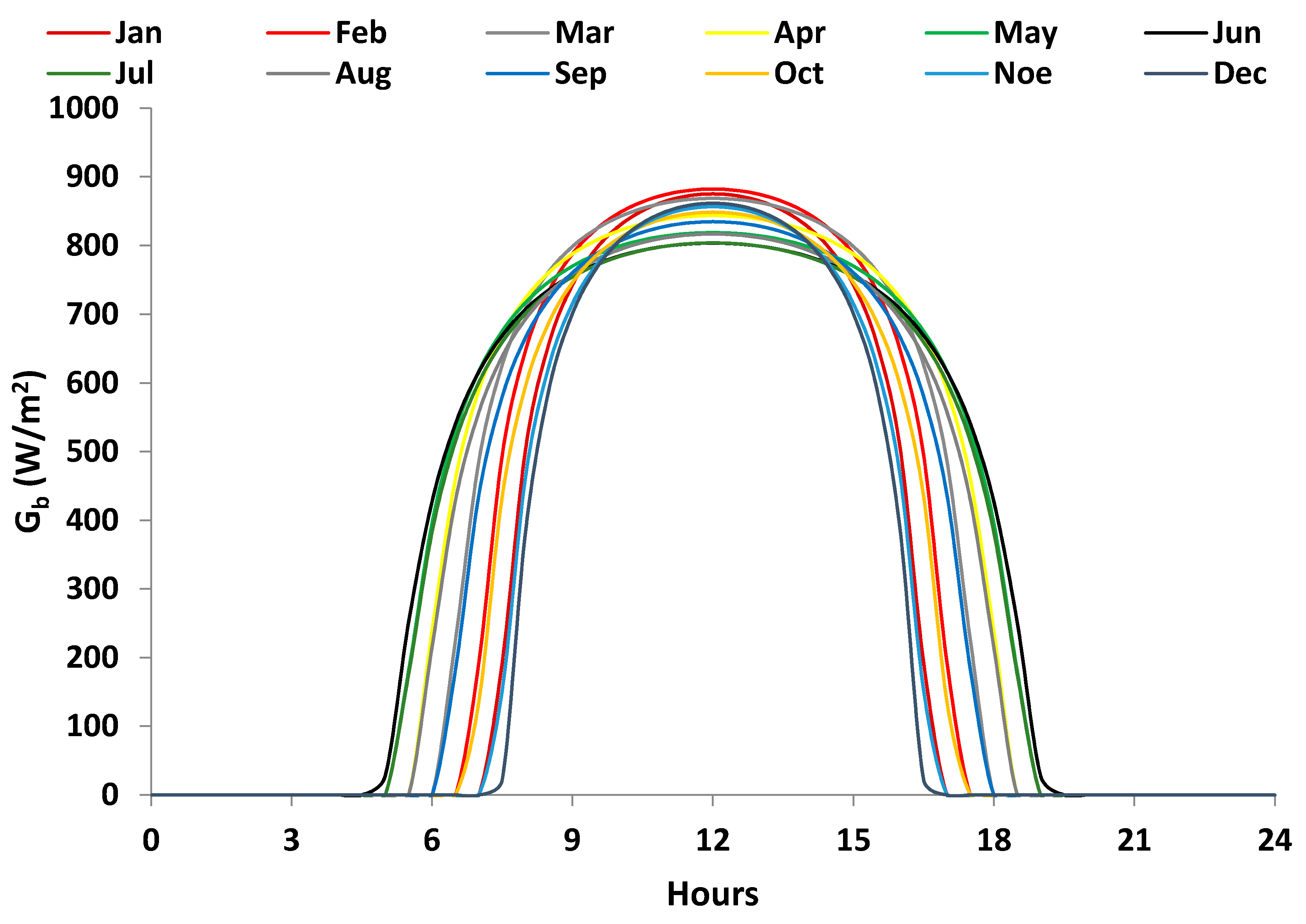
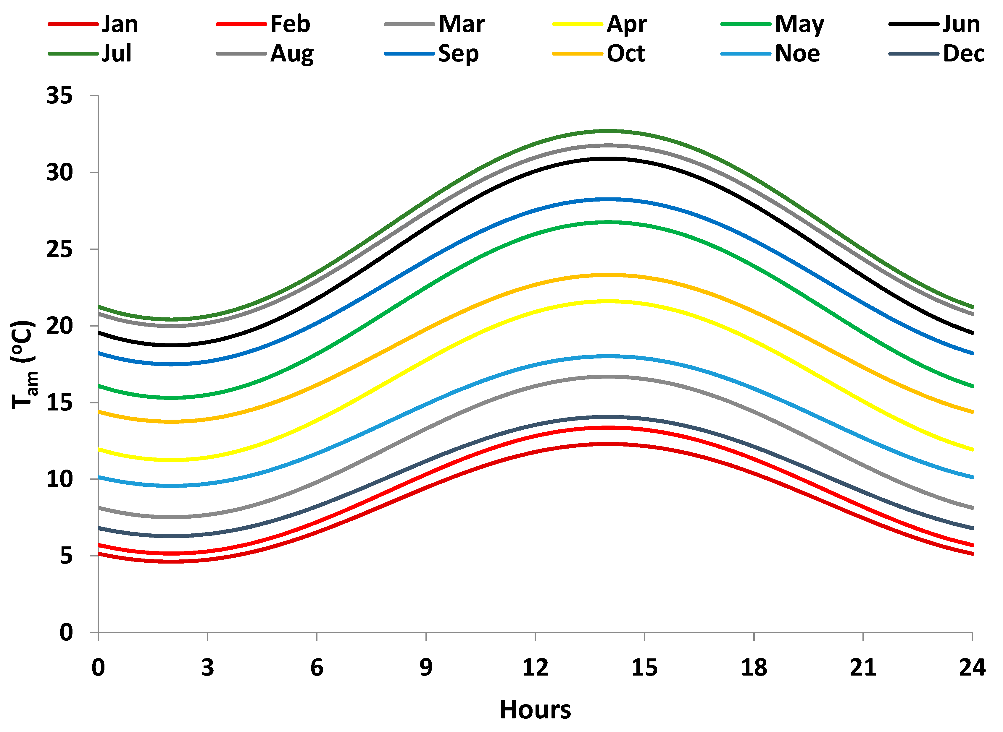
The system is investigated with a usual methodology by investigating 12 typical days, one for every month. Moreover, the system is assumed to operate only on the sunny days of every month. The examined weather data regards the climate conditions of Athens (Greece) with 38° latitude. The direct solar beam irradiation is given in Figure 2, and the ambient temperature in Figure 3. These results have been also given in [30], which is one previous work about PTC. The methods for obtaining these weather data are given in [30], and it is essential to state that the followed methodology is in accordance with the ASHRAE standards [34]. 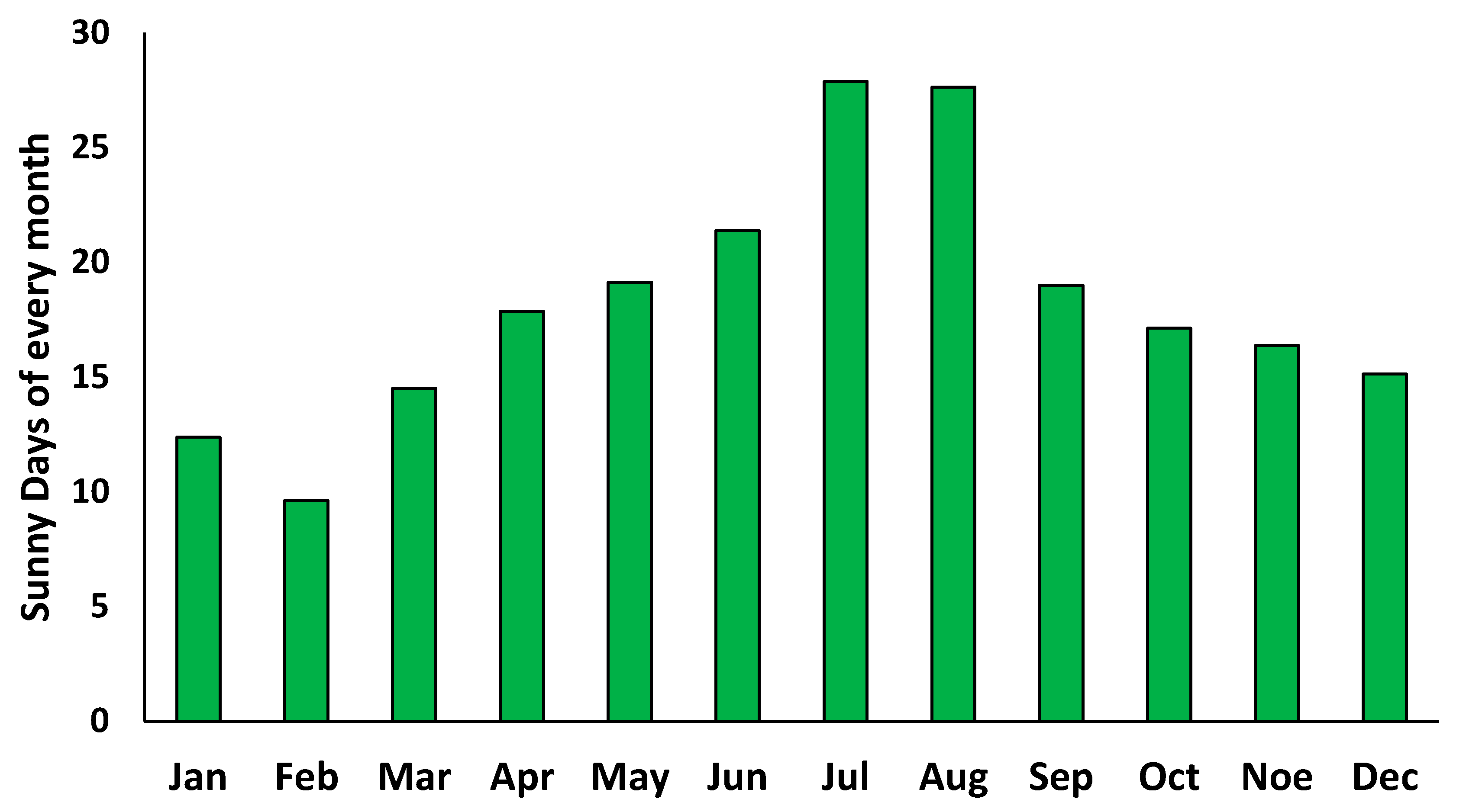Figure 4 exhibits the sunny days of every month, as they have been calculated using real-averaged meteorological data for the years 2010–2016 [35,36,37]. Totally, the solar system operates about 219 days per year, which is a reasonable percentage of 60%. This strategy has been also followed in [38] for a system with PTC.

2.7. Financial Analysis

In the present work, the financial analysis is a critical part because the industries are interested in financially viable investments. This work investigates the system with various financial indexes that are defined in this section. First of all, the total cost of the system (K_tot) is calculated. This parameter is depended on the collector field cost, the storage tank cost, and the heat exchanger cost:

$$K_{tot}=A_a\cdot K_c+V\cdot K_V+K_{hex}$$

(14)

The yearly cash flow (CF) is calculated by the energy that the solar collector gives to the industry (E_l,s), the cost of the heat (K_heat), and the cost of the operation and maintenance (K_O&M).

$$CF=E_{l,s}\cdot K_{heat}-K_{O\&M}$$

(15)

The cost of the operation and maintenance (K_O&M) is assumed to be the 1% of the capital cost of the system [39]:

$$K_{O\&M}=0.01\cdot K_{tot}$$

(16)

The net present value (NPV) of the investment is calculated as:

$$NPV=-K_{tot}+R\cdot CF$$

(17)

The equivalent years of the investment (R) are calculated as below:

$$R=\frac{{\left(1+r\right)}^N-1}{r\cdot {\left(1+r\right)}^N}$$

(18)

The payback period (PP) of the investment is calculated as:

$$PP=\frac{\ln \left(\frac{CF}{CF-r\cdot K_{tot}}\right)}{\ln \left(1+r\right)}$$

(19)

The internal rate of return (IRR) of the investment can be calculated by using the following (non-linear) expression:

$$IRR=\frac{CF}{K_{tot}}\cdot \left(1-\frac{1}{{\left(1+IRR\right)}^N}\right)$$

(20)

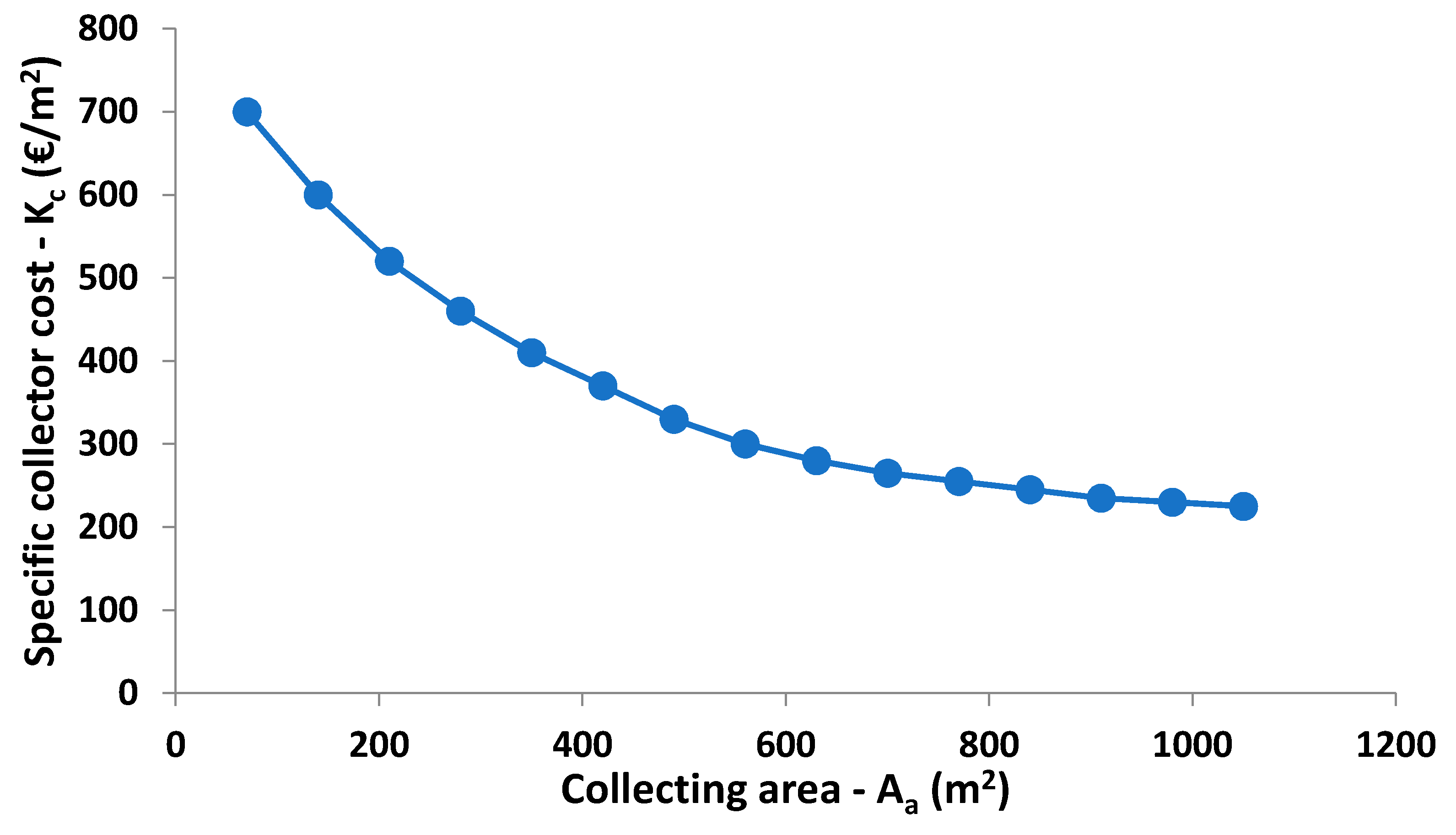
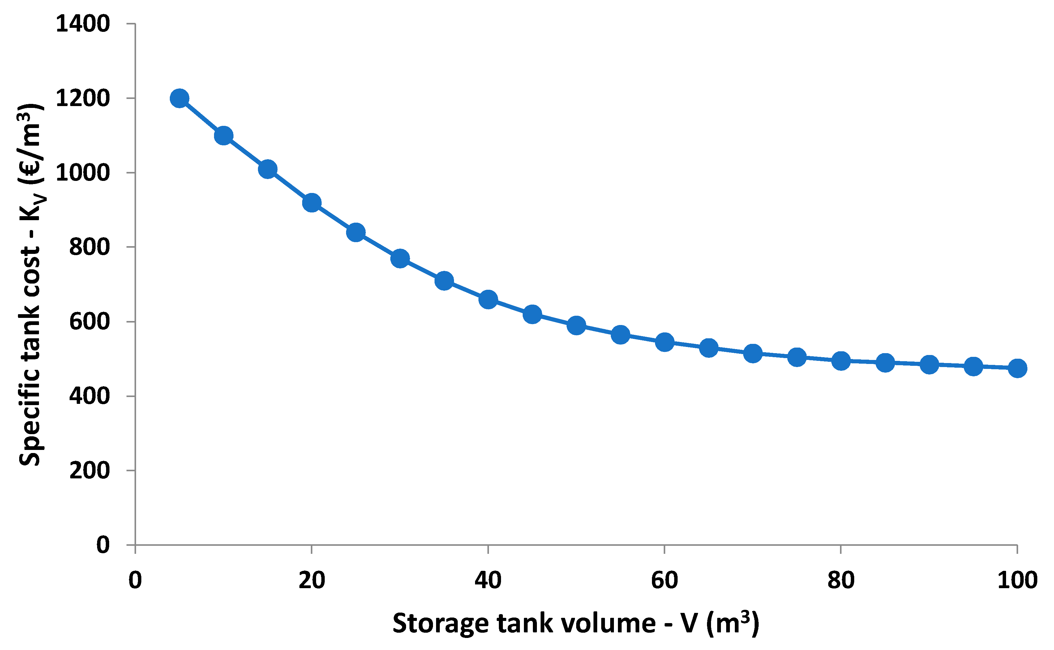
In this work, the collecting area (A_a) and the storage tank volume (V) are examined parametrically. According to the economy of scale theory, a higher quantity of a product has a lower specific cost for reasonable production. So, two curves for the specific cost of the collecting are and the storage tank volume are given in Figure 5 and Figure 6 respectively. These data correspond to reasonable selections according to the market prices. In the real installations, standard equipment has to be used for both too small or too great installations, which makes the specific cost lower for greater installations. For example, the control system, the piping, the tracking mechanism, etc., are not so different for small and great installations, and this is the main reason for using the costs listed in Figure 5 and Figure 6 in this work. These costs correspond to reasonable market costs, in which costs are really different between small and great installations [39,40,41].

Table 3. Data for the financial analysis.

Parameter	Symbol	Value
Heat exchanger cost	Khex	10 k€
Specific collector cost	Kc	225~700 €/m2
Specific tank cost	KV	475~1200 €/m3
Heat cost	Kheat	0.10 €/kWh
Project life	N	25 years
Discount factor	r	3%
O&M costs	KO&M	1%∙Ktot

includes the other parameters of this work. The heat exchanger cost is selected at 10 k€ [42], the project lifetime (N) is 25 years, and the discount factor (r) is 3% [38]. The cost of the heat is estimated to be 0.10 €/kWh [43]. Moreover, the range of the specific costs about the solar collectors and the storage tank are given in this table, as they have also presented in Figure 5 and Figure 6. It is essential to state that the installation cost is assumed to be included in the specific costs of Figure 5 and Figure 6.

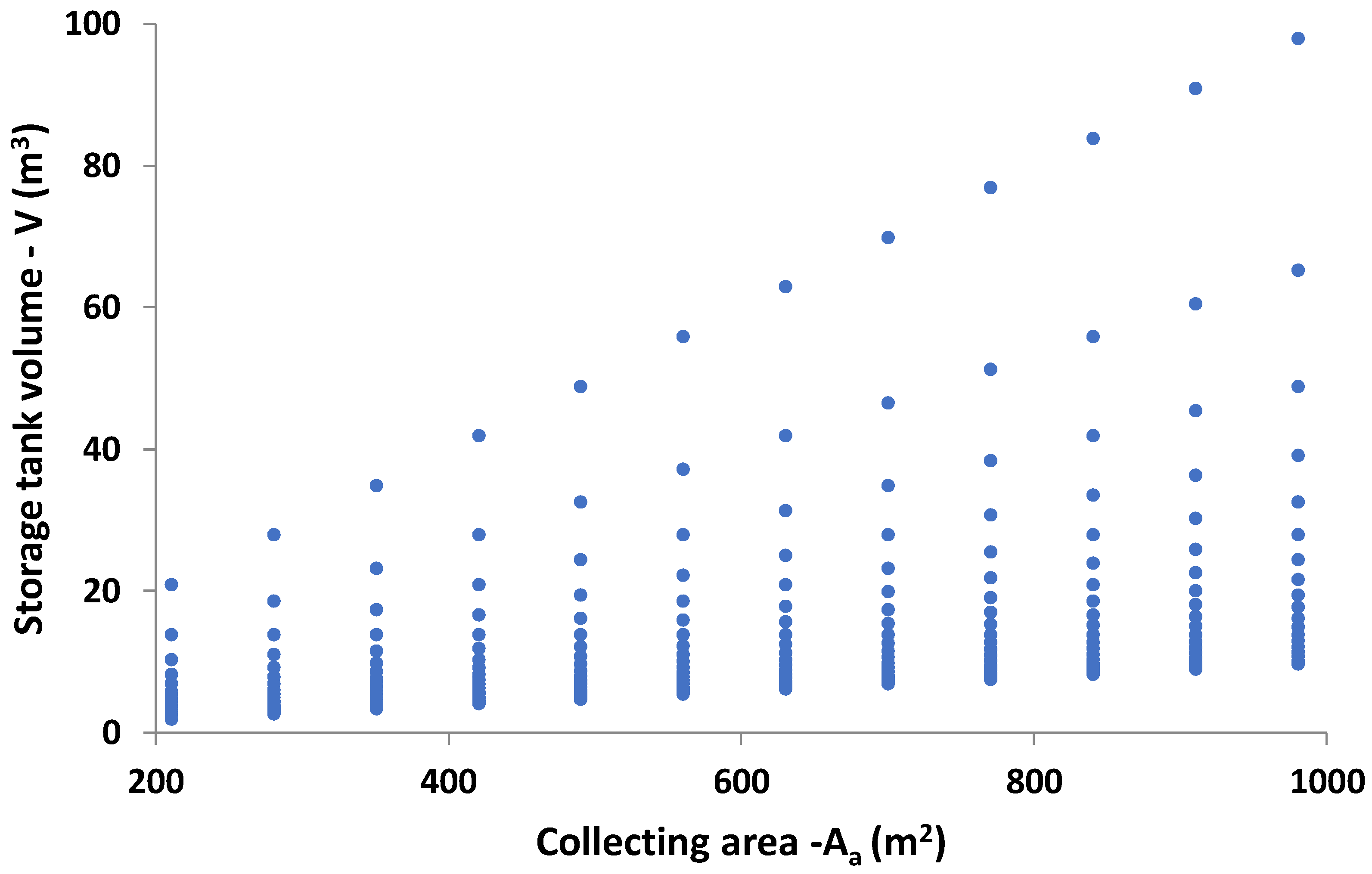
2.8. Followed Methodology

In this work, the industrial heat process system is optimized for five different heat production temperature levels (100 °C, 150 °C, 200 °C, 250 °C, 300 °C). For every case, the optimization variables are the collecting area (A_a) and the ratio of the collecting area to the storage tank (A_a/V). The collecting area ranged from 210 m² (3 modules) to 980 m² (14 modules), while the ratio (A_a/V) ranged from 10 m²/m³ up to 100 m²/m³. The collecting area is examined for a different number of modules, and so every extra module adds an extra 70 m² to the total collecting area. The reason for using the ratio (A_a/V) and not directly the volume (V) is based on the examination of the proper volumes in every case. More specifically, there is no reason for examining an extremely great tank for the case of three modules, because these tanks are suitable for cases with 10 modules, for instance. So, the present technique leads to the examination of the proper cases. Figure 7 shows the examined combination in a two-dimensional (2D) depiction.

The optimization is performed by examining all of the depicted cases in Figure 7, and then searching for which combinations leads to the optimum value for the objective function. Three different optimization procedures are performed:

(a)

Maximization of the solar cover (f)

(b)

Maximization of the net present value (NPV)

(c)

Minimization of the payback period (PP)

More specifically, three independent optimization procedures are performed, and the optimization goals in every case are given in the previous bullets (a to c). In every procedure, totally 228 cases are investigated, which are depicted in Figure 7. More specifically, 12 different collecting areas are examined, and for every collecting period, 19 different storage tanks are investigated. Finally, all of the cases are evaluated, and the one that satisfies the optimization goal is selected as the optimum one. For instance, for the first optimization procedure, the optimum case is the one that leads to maximum solar cover. In the second optimization procedure, the optimum case is the one with the maximum net present value, while in the third optimization procedure, the optimum case is the one with the lowest payback period.

The last step is the discussion of the optimum designs with the different criteria. The solar coverage is an energy criterion that indicates the amount of useful energy production by the sun. Higher values of this parameter indicate that higher amounts of the heat process load are cover by the solar energy, and so the auxiliary energy consumption is lower. The (NPV) and the (PP) are the financial criteria that evaluate the viability of the project. The (NPV) evaluates the total net gain of the investment if the capital cost, the yearly cash flow, the discount factor, and the total life of the project are taken into consideration. The payback period takes into account the capital cost, the yearly cash flow, and the discount factor, while the total project life is not considered in this index. The optimization with these criteria is important in order to investigate the system by different points of view. The optimum designs are different because the solar cover maximization generally indicates greater systems in order for higher useful energy amounts to be produced. On the other hand, the financial criteria usually indicate smaller systems, which presents an efficient relationship between the system scale and the energy production.

It is useful to state that the IRR has not be used as an optimization goal because its maximization was equivalent to the minimization of the payback period, and thus there was not any reason for presenting a fourth optimization procedure.

Now, it is important to state how the dynamic analysis in general and the yearly simulation has been conducted. Every combination (collecting area, storage tank, and temperature level of the load) was examined separately for 12 typical days during the year. The sunny days for every month have been used, and finally, the total yearly operation was developed. For every day, the system was examined with a time step of 30 seconds. The differential equations of the storage tank have been solved, and the procedure was performed for three days in order for the results to converge. The initial values in the tank were assumed to be the same as the load temperature level, but these values are converged after running the code for some consecutive days. Moreover, it is important to state that the collector loop was operating when the thermal efficiency was positive. Furthermore, the solar system feeds the load when the temperature of the thermal oil is higher than the load and there is a minimum pinch point of ~5 K in the heat exchanger. The proper control functions have been used in the code for respecting these constraints. It is essential to state that this work has been performed with a developed program in FORTRAN. Similar programs for the simulation of solar-driven systems in time-depended conditions have been performed in [39,41]. It is also useful to state that the developed model is based on the differential equation in the storage tank, while the other parts have been modeled with simple formulas, which makes the present analysis a pseudodynamic problem. In the end,

Table 4. General information about this work.

Description/Parameters	Data/Information
Location	Athens (Greece), latitude φ = 38°
Collector type	PTC, Eurotrough module
Tracking system	One-axis, follow the sun east–west
Storage type	Sensible storage
Working fluid	Thermal oil (Therminol VP-1)
Heat process load	100 kW
Yearly operation period	350 days–8400 h
Load temperature level	From 100 to 300 °C (variable)
Collecting area (Aa)	From 210 to 980 m2
Aa/V	From 10 to 100 m2/m3
Heat exchanger efficiency (ηhex)	70%
Tank thermal loss coefficient (UT)	0.8 W/m2K

is given, which includes the main information about this work. This table summarizes information that was previously given in Section 2.

3. Results and Discussion

The examined configuration is optimized with three different procedures, and the optimization results are given in Section 3.1, Section 3.2, Section 3.3 and Section 3.4. The summary and the deeper discussion of the results are given in Section 3.4.

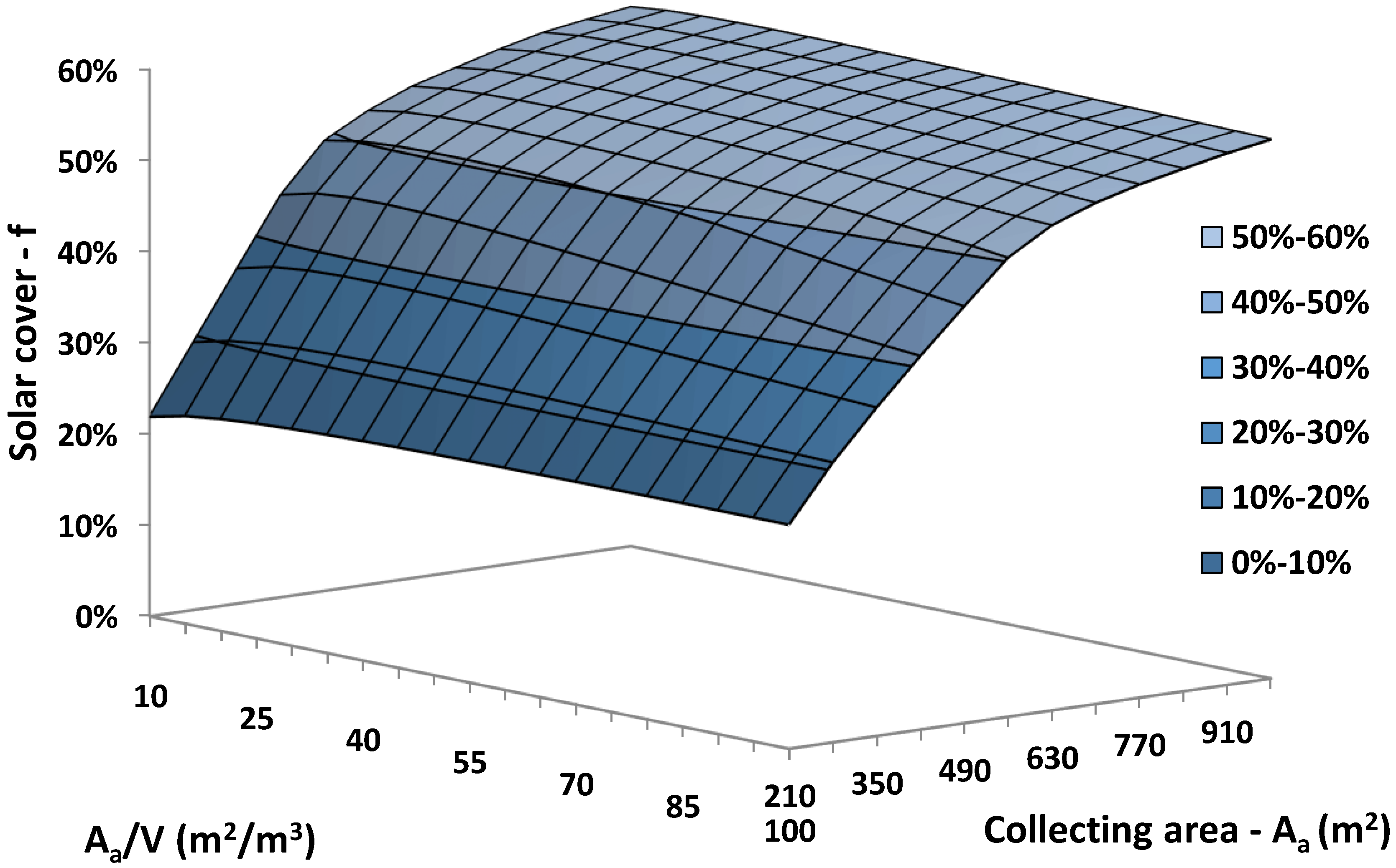
3.1. Optimization for Maximum Solar Cover

The first optimization procedure is performed with the maximization of the solar coverage as the goal. Figure 8 is a three-dimensional (3D) depiction of the solar coverage for the various examined cases with the load temperature level at 200 °C. This temperature level is selected as a representative intermediate temperature level. Generally, a higher collecting area leads to higher solar cover, which is reasonable. However, the optimum storage tank changes in every case. 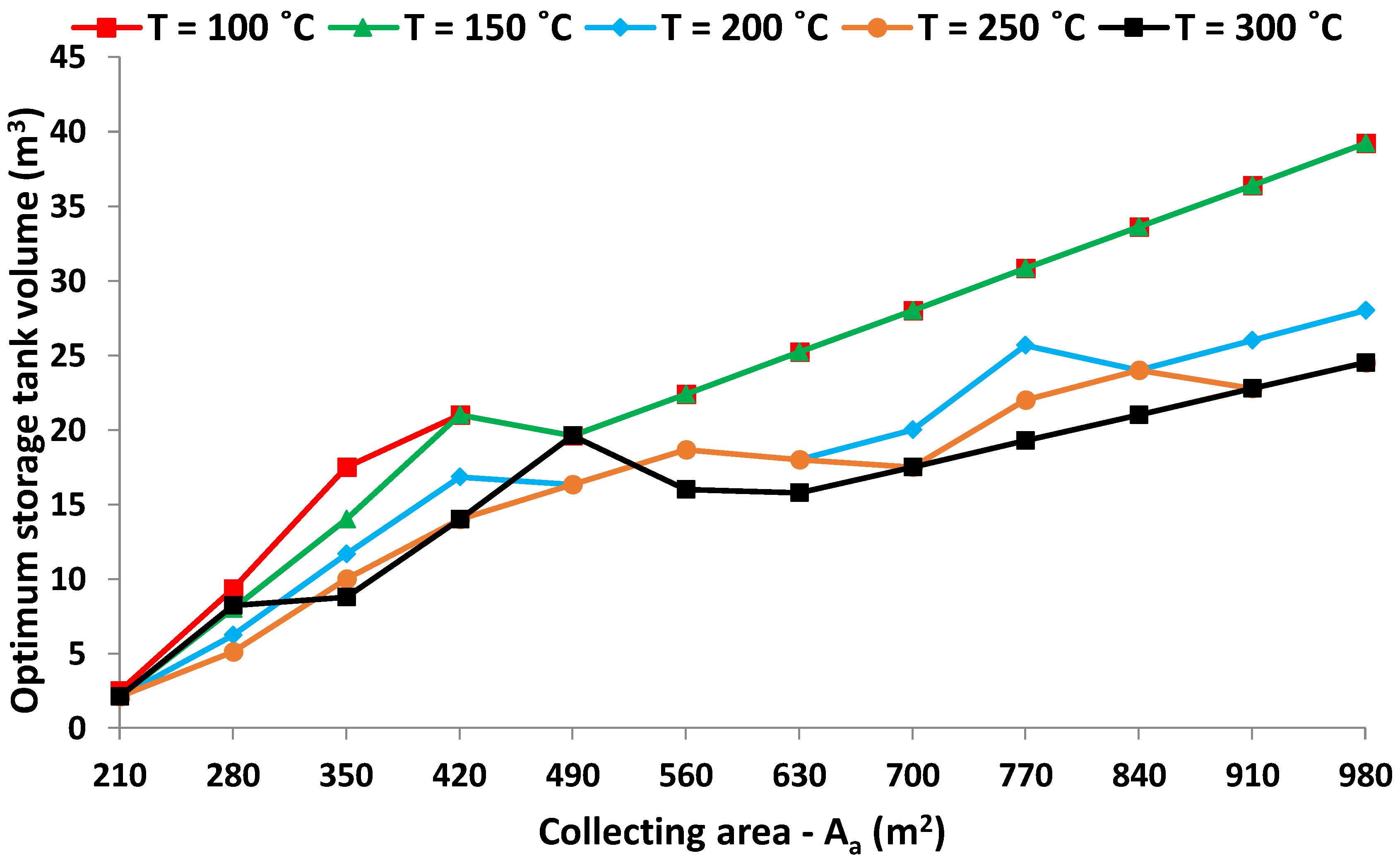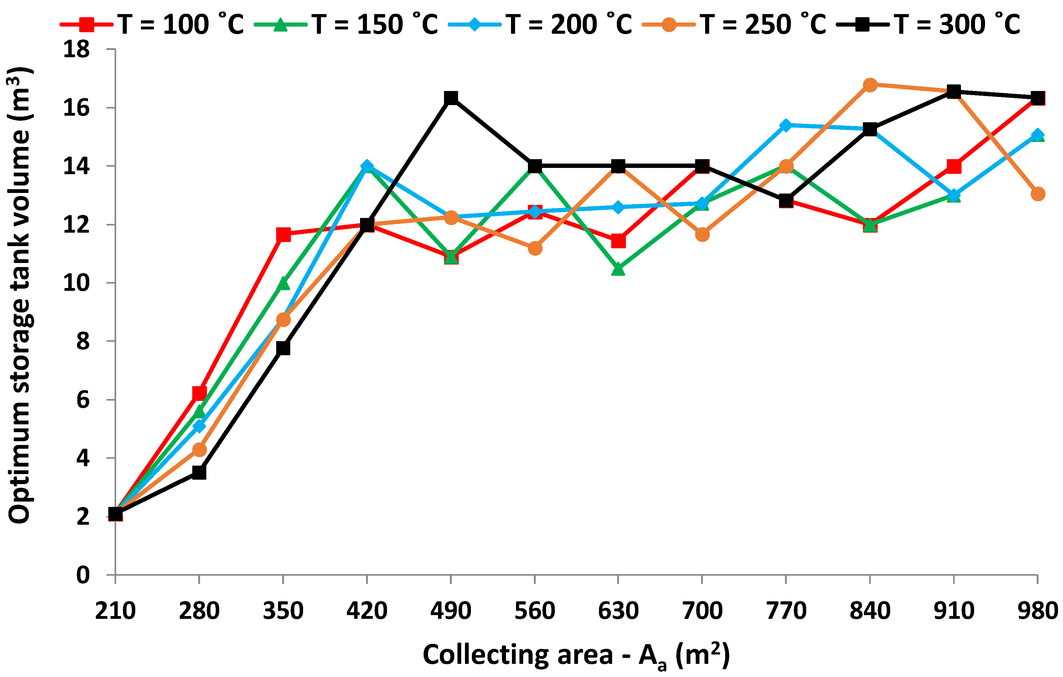Figure 9 illustrates the optimum storage tank volumes for different collecting areas, and for the six examined load temperature levels. The general sense is that higher collecting areas need higher storage tanks. Moreover, it is found that loads of higher temperatures need smaller tanks.

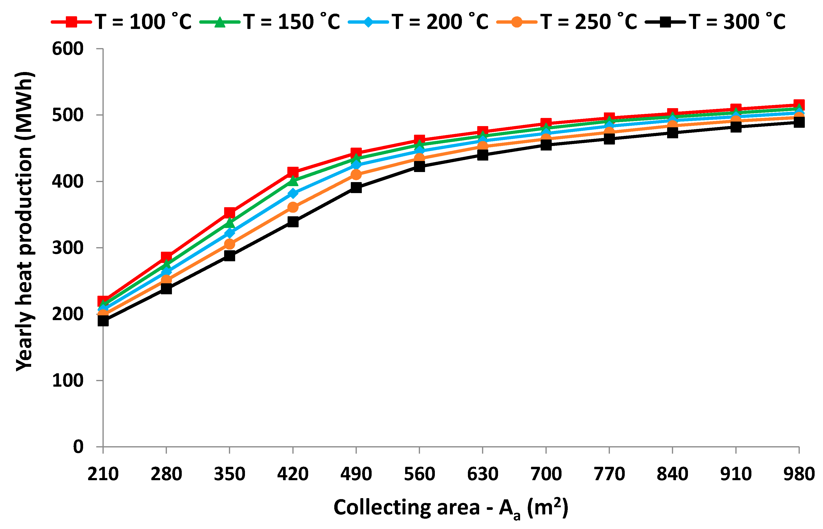
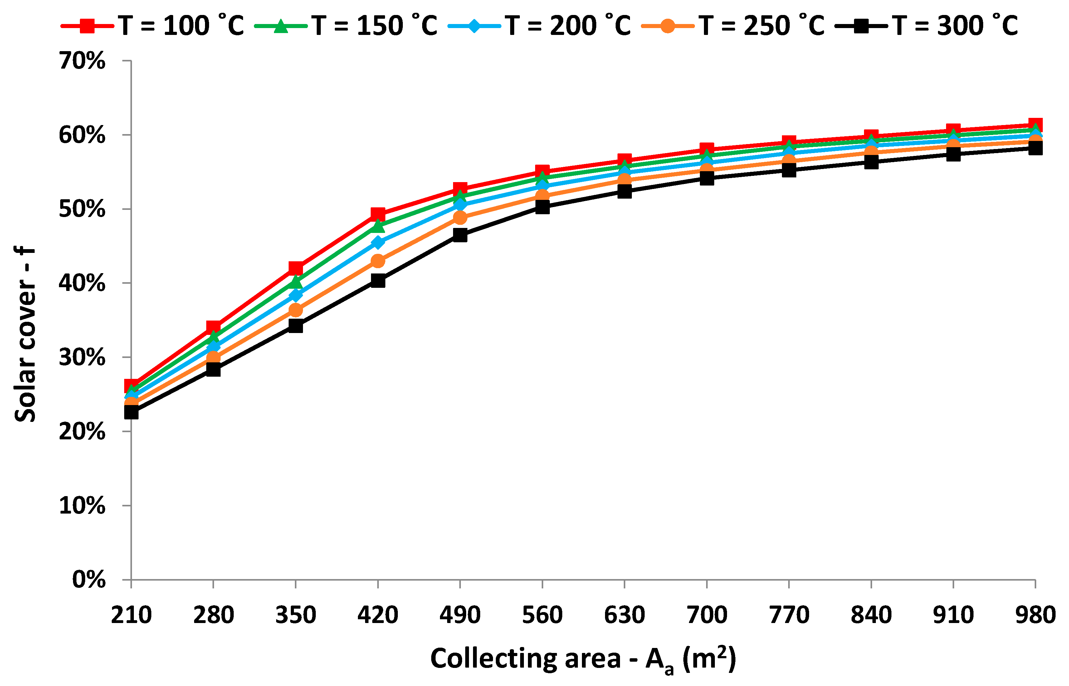
The yearly load production from the solar energy is given in Figure 10, and the respective solar cover is given in Figure 11. These results regard the cases with the optimum storage tank, as it has been given in Figure 9. It is obvious that higher collecting areas lead to higher cover and great production by the sun. Moreover, the solar cover is lower in higher load temperatures because the operation at higher temperatures leads to the reduction of the solar thermal efficiency. It can be said that after 560 m², the increasing rate in the solar cover is lower compared to the collecting areas for up to 560 m².

It is remarkable that the solar coverage reaches up to 60% approximately. This “upper limit” is reasonable if the maximum yearly operation days are considered. In other words, the sunny days of the year are 219 for Athens, and according to the used data, the operation days are 350 for the industry. The ratio of 219 to 350 gives a maximum solar cover of 62.57%, which is a bit higher than the obtained results. So, it is found that the examined configuration is able to cover the heat load on sunny days in a suitable way. More results about the monthly variation of the solar coverage are given in Section 3.4, which follows.

3.2. Optimization for Maximum NPV

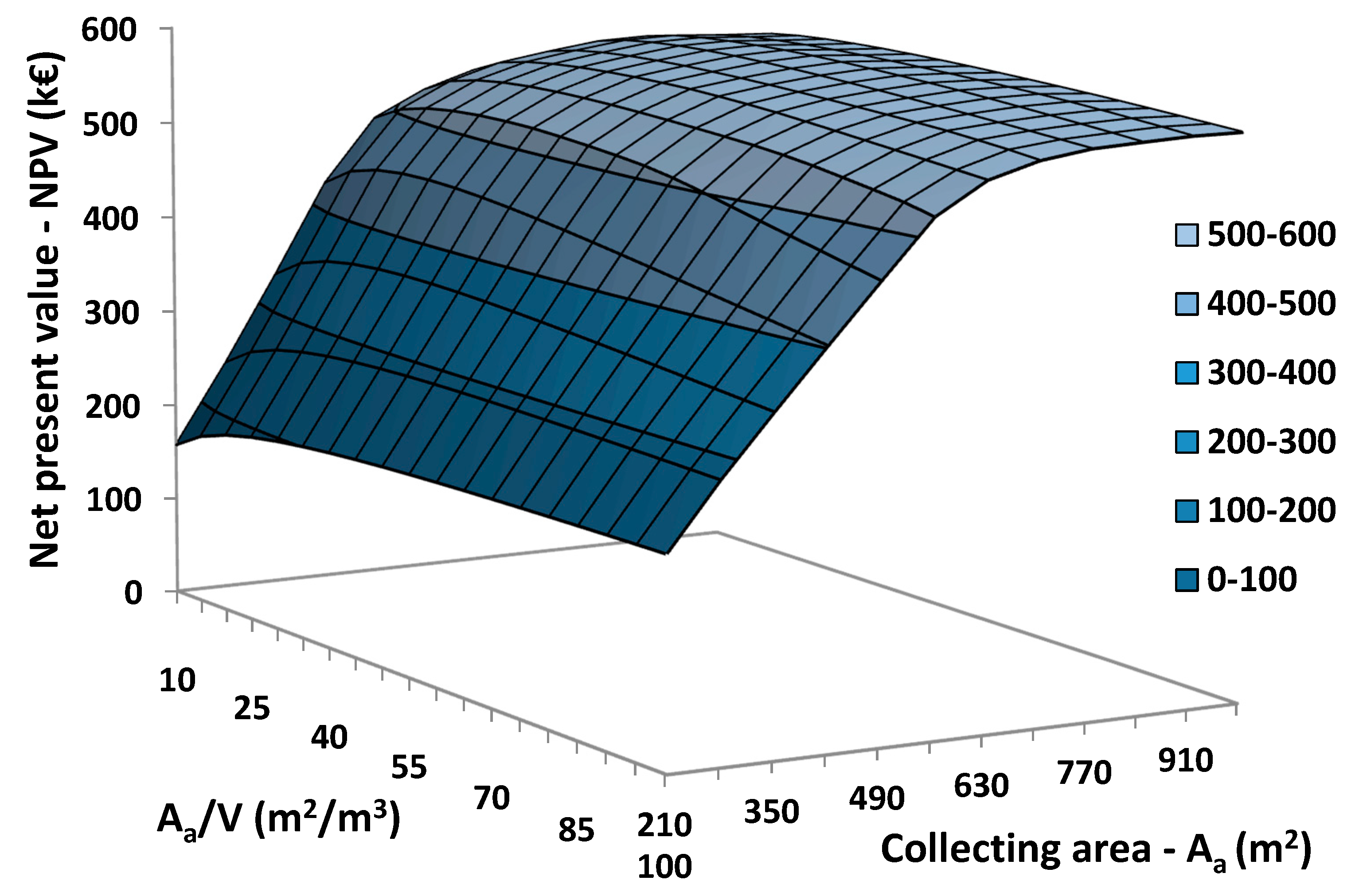
The second optimization procedure is based on the maximization of the NPV. This parameter is crucial for the investigation of the investment, and Figure 12 illustrates its variation with the optimization variables with the load temperature to be 200 °C. Generally, the NPV reaches close to 600 k€, and it is higher for great collecting areas. Also, the storage tank seems to play an important role in the results. Thus, Figure 13 gives the optimum storage tank volumes for different collecting areas and temperature levels. Generally, a higher collecting area needs a higher storage tank, but after 490 m², the optimum storage tank is close to 15 m³.

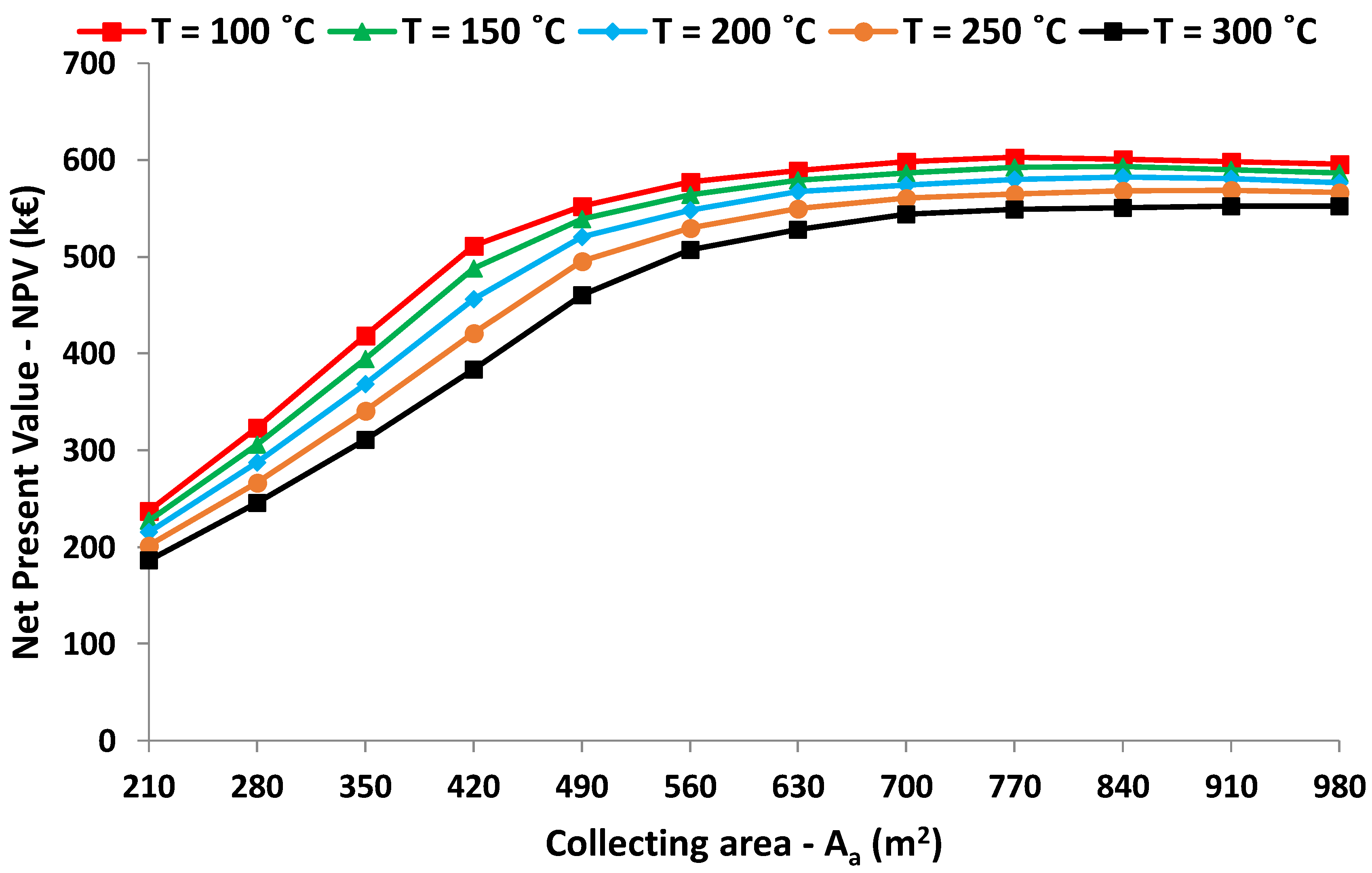
Figure 14 depicts the NPV for different temperature levels and collecting areas with the optimum storage tanks as they have been defined in Figure 13. The NPV has an increasing rate with the collecting area, which is maximized for collecting areas between 770 m² (for T_l = 100 °C) and 980 m² (for T_l = 300 °C). It is important to state that after 630 m², the NPV has small variations with the collecting area. Moreover, it has to be said that the cases with higher temperature levels have lower NPV, because the heat cost is the same in all of the cases, and the collector thermal efficiency is lower at higher temperature levels.

3.3. Optimization for a Minimum Payback Period

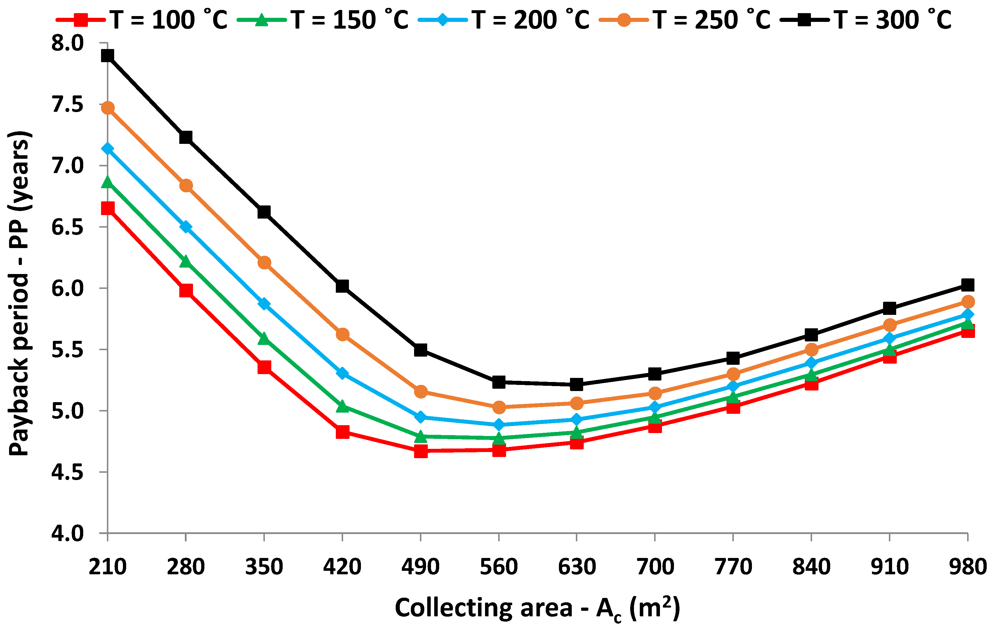
The third optimization procedure is conducted with the minimization of the payback period as the criterion. This parameter is important, and it is used in many cases in order to evaluate choices such as the use of solar energy for covering a load and substituting partially the conventional fossil fuel boiler.

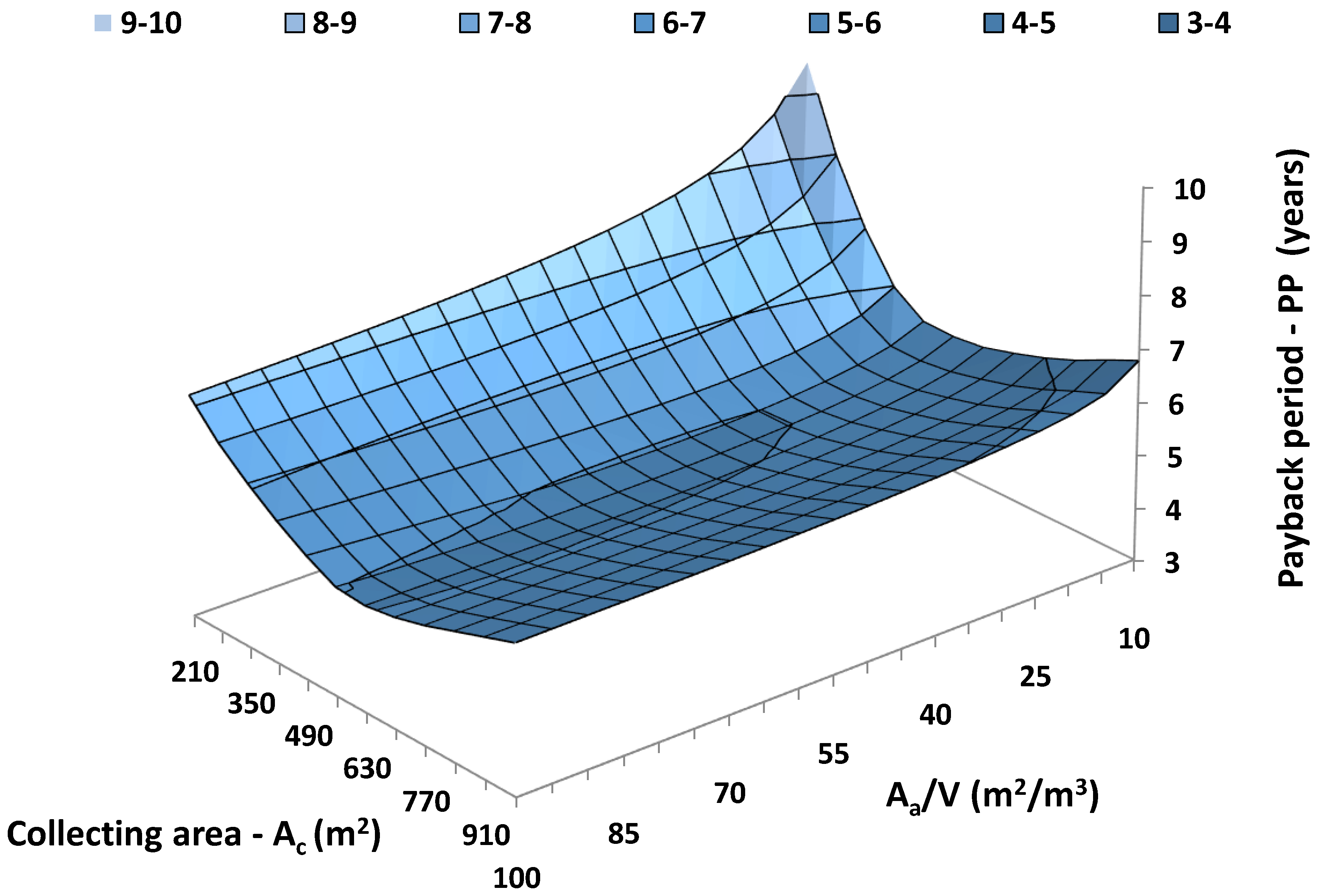
Figure 15 is a 3D depiction of the simple payback period with the optimization variables when the load is at 200 °C. This Figure clearly shows the existence of a global minimum point at 560 m² collecting area with an 8-m³ storage tank volume [or (A_a/V) = 70 m²/m³]. In this case, the payback period is 4.88 years, which is a promising value, especially for renewable energy technologies.

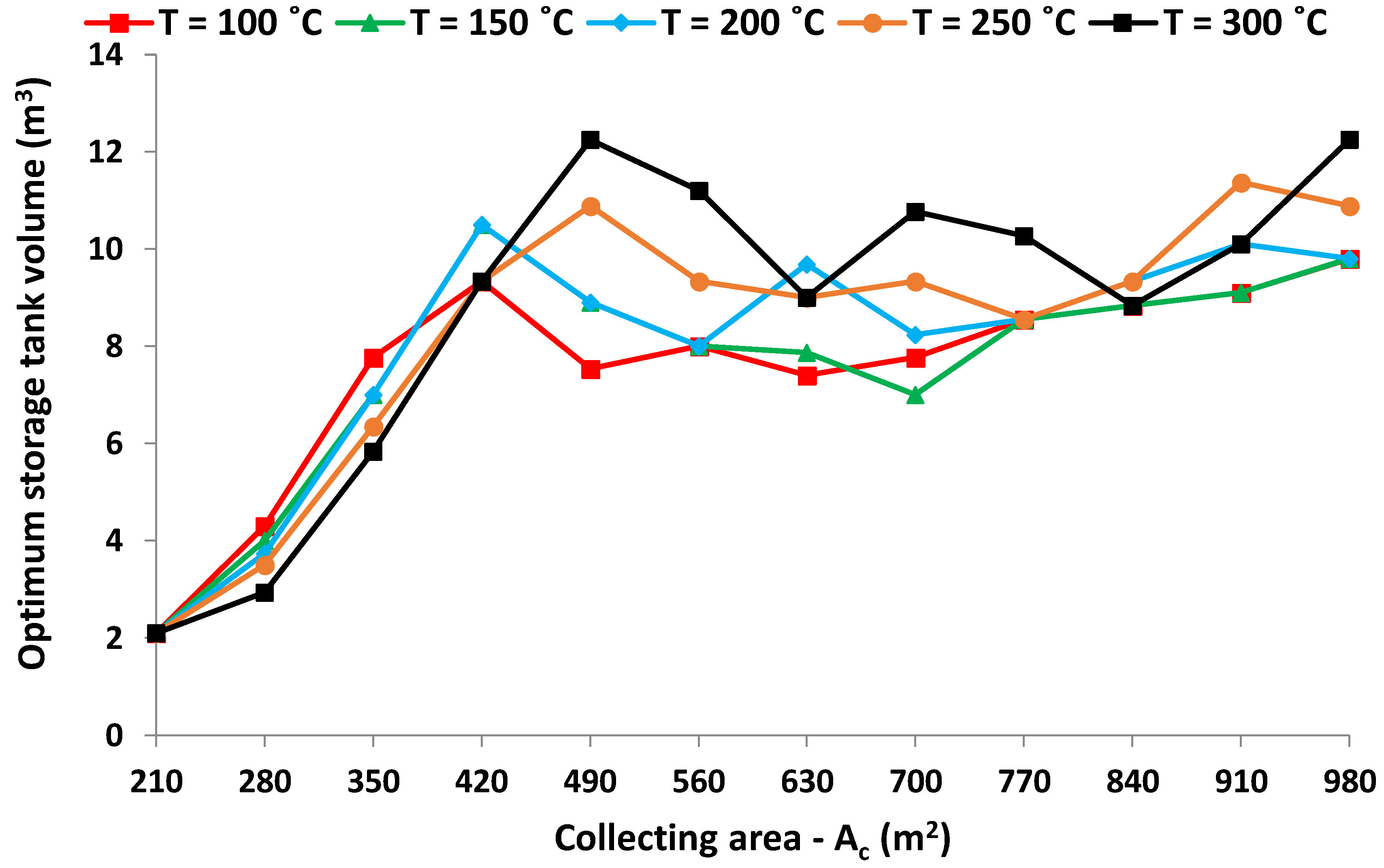
Figure 16 exhibits the optimum storage tanks for different load temperatures and collecting areas. The optimum storage tank is about 10 m³ for the majority of the cases. Figure 17 gives the payback period for all of the load temperatures, and for the examined collecting areas with the optimum storage tanks in every case. The payback period is minimized at 560 m² for all of the temperature levels except 300 °C, which is minimized for 630 m². These results indicate that there is a great influence of the collecting area to the minimization of the payback period. This result was not found in the optimization of the system with the maximization of the NPV, because in this case, there was a great “optimum area” where the NPV presented a small variation.

3.4. Summary and Discussion

The last step in this investigation is the comparisons and the discussion of the obtained results.

Table 5. Optimization results for solar cover maximization (Scenario A). NPV: net present value, PP: payback period, IRR: internal rate of return.

Tl	Aa,opt	(Aa/V)opt	Vopt	NPV	PP	IRR	fmax
(°C)	(m2)	(m2/m3)	(m3)	(k€)	(Years)	(%)	(%)
100	980	25	39.2	589	5.95	18.32	61.34
150	980	25	39.2	578	6.03	18.09	50.65
200	980	35	28.0	572	6.01	18.15	59.89
250	980	40	24.5	562	6.06	18.00	59.08
300	980	40	24.5	549	6.16	17.71	58.21

,

Table 6. Optimization results for NPV maximization (Scenario B).

Tl	Aa,opt	(Aa/V)opt	Vopt	NPVmax	PP	IRR	f
(°C)	(m2)	(m2/m3)	(m3)	(k€)	(years)	(%)	(%)
100	770	60	12.8	603	5.07	21.38	58.78
150	840	70	12.0	593	5.31	20.64	58.91
200	840	55	15.3	582	5.44	19.99	58.37
250	910	55	16.6	569	5.75	18.95	58.35
300	980	60	16.3	552	6.06	18.01	58.02

and

Table 7. Optimization results for payback period minimization (Scenario C).

Tl	Aa,opt	(Aa/V)opt	Vopt	NPV	PPmin	IRR	f
(°C)	(m2)	(m2/m3)	(m3)	(k€)	(years)	(%)	(%)
100	560	70	8.0	573	4.68	23.09	54.27
150	560	70	8.0	559	4.78	22.79	53.30
200	560	70	8.0	543	4.88	22.17	52.26
250	560	60	9.3	527	5.03	21.73	51.26
300	630	70	9.0	525	5.21	21.02	51.69

include the results of the global optimum cases with the three performed optimization procedures, as they have been described in Section 3.1, Section 3.2 and Section 3.3 in detail. These tables give results about the optimum design (collecting area and storage tank), as well as the values of the crucial parameter for these cases. These results regard all of the examined load temperature levels.

It can be said that the optimum design is different when the different optimization criteria are used. This creates many optimum scenarios, and this result needs more investigation. The optimization with the solar cover lead to the maximum examined collecting areas (980 m²), while the NPV gives values that are a bit lower, from 770 m² to 980 m². The optimization with the PP gives significantly lower collecting areas between 560–630 m².

At this point, the case of 200 °C is selected as an example in order to make a suitable analysis. Using the solar cover as a criterion (scenario A), the solar cover is 59.89%, the NPV is 572 k€, and the payback period is 6.01 years. Using the NPV as a criterion (scenario B), the solar cover is 58.37%, the NPV is 582 k€, and the payback period is 5.44 years. Moreover, using the payback period as a criterion (scenario C), the solar cover is 52.26%, the NPV is 543 k€, and the payback period is 4.88 years. These results show that the use of solar cover as criterion leads to a relatively high payback period (6.01 years from 4.88 years), while the use of the payback period leads to lower solar cover (52.26% from 59.89%). However, the use of NPV as criterion leads to a small sacrifice in solar cover (58.37% from 59.89%) and payback period (5.44 years from 4.88 years). So, the optimum design according to the NPV seems to be the most suitable case. In this scenario, the collecting area is 840 m², and the storage tank volume is 15.3 m³.

It is also useful to state that the optimum collecting areas are generally higher for higher load temperatures. Moreover, the optimum storage tanks are lower in higher temperatures for optimization with solar cover, while they are higher for optimization with financial criteria.

The optimization with the solar cover leads generally to greater storage tanks (24.5 m³ to 39.2 m³), the optimization with the NPV leads to intermediate storage tanks volumes (12.8 m³ to 16.3 m³), while the optimization with the payback period leads to the smallest tanks (8 m³ to 9 m³). At this point, it is important to state that the literature results of Table 1 are generally found with energetic optimizations, and thus the found storage tanks are generally great, which is also obvious from the previous comparative discussion.

The IRR is also given in Table 5, Table 6 and Table 7. It takes values from 17.71 to 23.09%, which are satisfying values. This parameter has not been used as an optimization goal, because the IRR maximization was found to be equivalent to the minimization of the payback period.

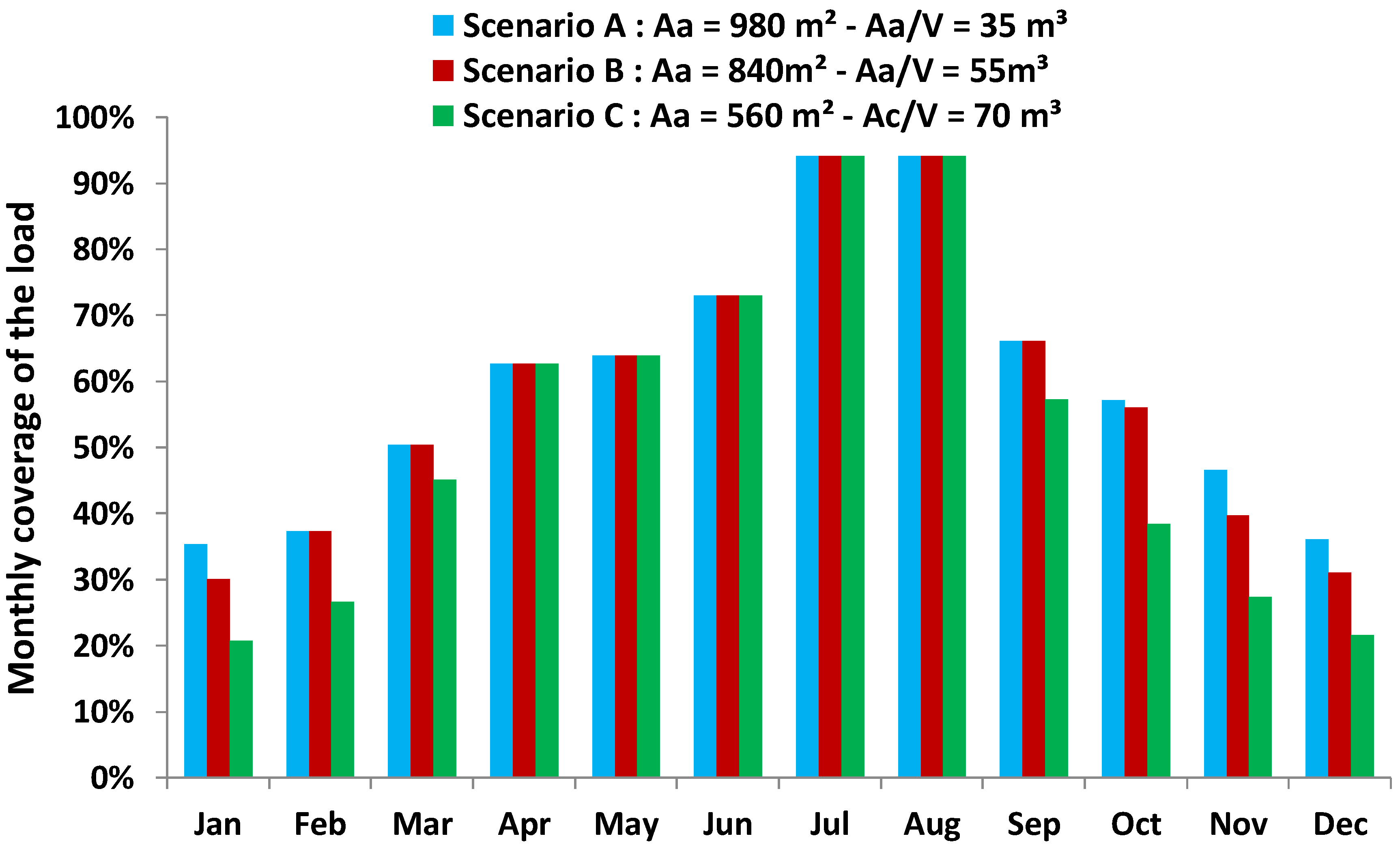
The last step in this work is the presentation of the monthly results for the solar coverage of the load. These results are depicted in Figure 18, and they regard the three optimum cases for the load temperature of 200 °C. The solar cover has the same values among the three scenarios from April to August. This shows that increasing the collecting area is not beneficial during these months. However, the greater collecting areas of scenario A and B gives higher solar cover than the scenario C for the rest of the year. During the winter, solar coverage of 20~30% is achieved, while in July and August, it reaches close to 90%. The main reason for these results is the number of the sunny days of every month. It is important to state that the days without operation (15 per year) are assumed to be separated in all of the months in the same way. This assumption gives the proper time for maintenance during the entire year. Moreover,

Table 8. Energy production during the months and the year for the three optimum scenarios.

Period	Energy Production by the Solar Energy (MWh)
	Scenario A	Scenario B	Scenario C
January	25.23	21.49	14.84
February	24.00	24.00	17.10
March	36.00	36.00	32.17
April	43.20	43.20	43.20
May	45.60	45.60	45.60
June	50.40	50.40	50.40
July	67.20	67.20	67.20
August	67.20	67.20	67.20
September	45.60	45.60	39.47
October	40.80	39.99	27.43
November	32.09	27.41	18.94
December	25.75	22.20	15.39
Year	503.07	490.29	438.95

includes the monthly energy production by the solar energy for the three optimum scenarios.

4. Conclusions

The objective of this work is the energetic and financial optimization of a solar heat industrial process system. Parabolic trough solar collectors coupled to a storage tank are used in order to cover a continuous industrial heat load. The temperature of this load is examined parametrically from 100 °C to 300 °C, covering a great range of possible applications as they have been described in the introduction section. The optimization is performed with three different procedures with the following criteria: maximization of the solar cover, maximization of the NPV, and minimization of the payback period. The optimization variables were the collecting area and the storage tank volume. This analysis regards the climate conditions of Athens (Greece) and the load was selected at 100 kW. The most important conclusions of this work are summarized below:

-

Higher load temperatures lead to greater optimum collecting areas, lower solar cover, lower NPV, and a higher payback period.

-

The optimum storage tank is greater when the system is optimized with energy criteria (solar cover) compared to the financial optimization (NPV and payback period).

-

The solar cover was generally found close to 60%, which is a high value. This value is restricted by the number of the sunny days during the year.

-

Different criteria lead to the different optimum scenario. Finally, the optimization with the NPV maximization is found to be the most suitable case. In this scenario with a temperature load of 200 °C, the collecting area is 840 m², the storage tank volume is 15.3 m³, the NPV is 582 k€, and the solar cover is 58.37%.

-

The IRR was found to range from 17.71 to 23.09%, which are acceptable and promising values for the present technology.

In the end, it can be said that the use of PTC for industrial heat process of various temperature levels is a financially viable investment with good indexes and high solar coverage.