Article

Computational Analysis of Tricuspid Heart Valves

Biomedical, Industrial and Human Factors Engineering, Wright State University, 3640 Col. Glen Hwy, Dayton, OH 45325, USA
*
Author to whom correspondence should be addressed.
Designs 2026, 10(3), 57; https://doi.org/10.3390/designs10030057
Submission received: 31 March 2026 / Revised: 14 May 2026 / Accepted: 14 May 2026 / Published: 19 May 2026
(This article belongs to the Section Bioengineering Design)

Abstract

Understanding the mechanical behavior of valve materials and the hemodynamic characteristics of blood flow is important for improving prosthetic heart valve design. In this study, a comprehensive computational investigation was conducted to evaluate the biomechanical and hemodynamic behavior of a three-dimensional tricuspid valve model constructed from reported prosthetic valve geometries. The structural response of the valve was evaluated using linear elastic, viscoelastic, and hyperelastic constitutive models for four different materials: pyrolytic carbon, polyurethane, porcine tissue, and bovine tissue. The results demonstrated clear material-dependent trends. Pyrolytic carbon exhibited negligible deformation (1.7166 × 10⁻⁸ m), confirming its rigid mechanical behavior, whereas biological tissues showed greater compliance, with the largest deformation observed for the bovine hyperelastic model (9.6837 × 10⁻⁵ m). Hyperelastic tissue models produced lower peak von Mises stresses (1.3951 × 10⁴–1.8603 × 10⁴ Pa) than the corresponding linear elastic tissue models (2.6842 × 10⁴–2.7017 × 10⁴ Pa), indicating improved stress redistribution under nonlinear deformation. Polyurethane showed intermediate mechanical behavior, with moderate deformation and lower stress under viscoelastic modeling than under the linear elastic assumption, suggesting its potential as a polymeric alternative to traditional valve materials. The Computational Fluid Dynamics (CFD) analysis of the rigid open valve geometry revealed a central velocity jet with a peak velocity of approximately 0.092 m/s, localized vortex formation with a maximum vorticity magnitude of about 177 s−1 and a peak instantaneous wall shear stress of 1.32 Pa near the leaflet edges and valve opening. Overall, the results highlight the trade-off between rigidity, compliance, and durability among prosthetic valve materials and suggest that polyurethane may provide a balanced alternative for tricuspid valve replacement.

1. Introduction

The tricuspid valve, once referred to as the “forgotten valve” in cardiac research, has now become an area of interest in cardiovascular medicine, given the increasing incidence of tricuspid regurgitation and its significant impact on long-term survival [1,2,3]. Although surgical repair is generally considered the preferred treatment for tricuspid regurgitation, tricuspid valve replacement (TVR) becomes necessary in cases involving severe leaflet damage or when repair procedures fail [4,5]. Compared with the extensively studied aortic valve, the biomechanics of the tricuspid valve have received relatively less attention, partly because it operates under a lower-pressure environment.
Prosthetic heart valves are broadly classified into mechanical and bioprosthetic valves, each offering distinct advantages and disadvantages. Mechanical prosthetic heart valves, mainly composed of Pyrolytic Carbon (PyC), are highly valued for their durability, with a lifespan exceeding 25 years [6,7]. Nevertheless, the prothrombotic effects of mechanical heart valves, due to their mechanical composition, necessitate anticoagulant therapy, thereby increasing the risk of bleeding [4,8]. On the contrary, bioprosthetic heart valves, composed of xenogenic materials such as porcine valve tissue or bovine pericardium, are widely used due to their favorable hemodynamic performance and reduced risk of thromboembolic complications compared with mechanical valves, as they typically do not require lifelong anticoagulation therapy [9,10]. Bovine Pericardium has gained widespread use in modern prosthetic valves due to its high collagen content and favorable fatigue resistance [11]. Nevertheless, bioprosthetic heart valves are known to be prone to Structural Valve Deterioration (SVD), thereby limiting their lifespan to approximately 10–15 years [12].
To address the limitations of both mechanical and biological valves, significant research efforts have been directed toward the development of polymeric heart valves, particularly those based on polyurethane (PU) and other flexible polymeric materials. Polymeric valves aim to combine the durability of mechanical valves with the favorable hemodynamic performance of biological tissues [13,14]. Advances in thermoplastic polyurethane formulations have demonstrated promising mechanical properties, including high strain tolerance, fatigue resistance, and improved hemocompatibility. Recent experimental and computational studies suggest that polymeric valves may represent a promising alternative for next-generation prosthetic heart valve designs [15,16].
Understanding the interaction between prosthetic valve materials and cardiovascular flow conditions is essential for optimizing valve design and improving clinical outcomes. However, direct experimental evaluation of these interactions is challenging due to the complexity of cardiac hemodynamics and the difficulty of measuring stresses within valve leaflets during physiological operation. Consequently, computational modeling approaches, including finite element analysis (FEA) and computational fluid dynamics (CFD), have become widely used tools for investigating heart valve biomechanics. These methods enable detailed quantification of structural stresses, deformations, flow velocity fields, pressure gradients, and wall shear stresses that are not easily measured experimentally [17]. Recent computational investigations have demonstrated that integrated structural and fluid-dynamic simulations provide valuable insights into the biomechanical and hemodynamic behavior of prosthetic heart valves and can assist in optimizing valve geometry and material selection [18,19,20].
Computational modeling has become an essential tool for understanding valve biomechanics, enabling detailed evaluation of stress distributions, leaflet deformation, and flow patterns that are difficult to measure experimentally. Comprehensive reviews emphasize that finite element and fluid dynamic simulations are increasingly used to guide prosthetic valve design and clinical intervention planning [21]. Fluid–structure interaction simulations have further demonstrated that the mechanical properties of valve materials significantly influence leaflet deformation patterns, stress concentration regions, and downstream flow structures [22]. Recent experimental validations using physiologically inspired phantom models have further confirmed the reliability of these computational frameworks in capturing transient opening dynamics [23]. Also, recent patient-specific computational studies have shown that realistic modeling of valve geometry and material properties is critical for accurately predicting valve kinematics and hemodynamic performance [24].
Despite these advances, most computational investigations focus on a single material type or employ only one constitutive model, which limits the ability to directly compare the biomechanical performance of different prosthetic valve materials under identical physiological conditions. In particular, few studies have examined how different material classes, including rigid mechanical materials, flexible polymers, and biological tissues, affect valve deformation, stress distribution, and flow characteristics within a computational framework.
Therefore, the objective of this study is to perform a comparative structural analysis of four representative valve materials: pyrolytic carbon, polyurethane, porcine tissue, and bovine tissue using advanced computational modeling techniques. Transient structural simulations were conducted to evaluate deformation behavior, stress distribution, strain, and strain energy using appropriate constitutive models including linear elastic, viscoelastic, and hyperelastic formulations. In addition, computational fluid dynamics simulations were performed to analyze velocity distribution, vortex formation, pressure gradients, and wall shear stress within a tricuspid valve geometry. By systematically comparing the structural responses of these materials and studying the hemodynamic performance of the tricuspid heart valve, this study aims to provide deeper insight into the trade-offs between material stiffness, compliance, durability, and hemodynamic performance, thereby contributing to the development of improved prosthetic valve designs for tricuspid valve replacement.
The novelty of the present study lies in the unified computational comparison of four representative prosthetic-valve material classes within the same tricuspid geometry and loading framework. By combining linear elastic, viscoelastic, and hyperelastic constitutive descriptions with complementary structural and CFD analyses, the study enables direct assessment of how material behavior influences deformation, stress redistribution, strain energy, and simplified hemodynamic trends under consistent modeling assumptions.
These findings highlight the importance of material selection in balancing structural durability and physiological compliance in prosthetic tricuspid valve design.

2. Methodology

2.1. Geometry and Computational Domain

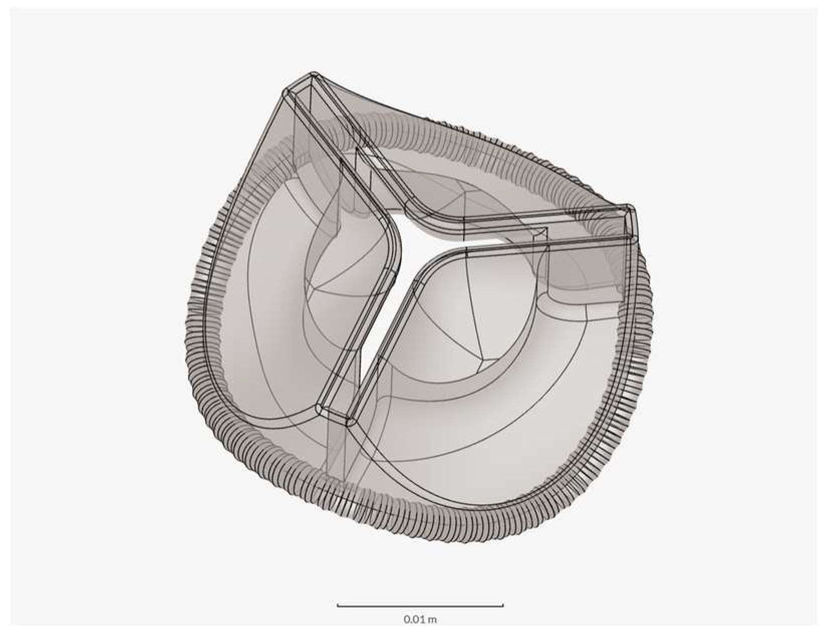
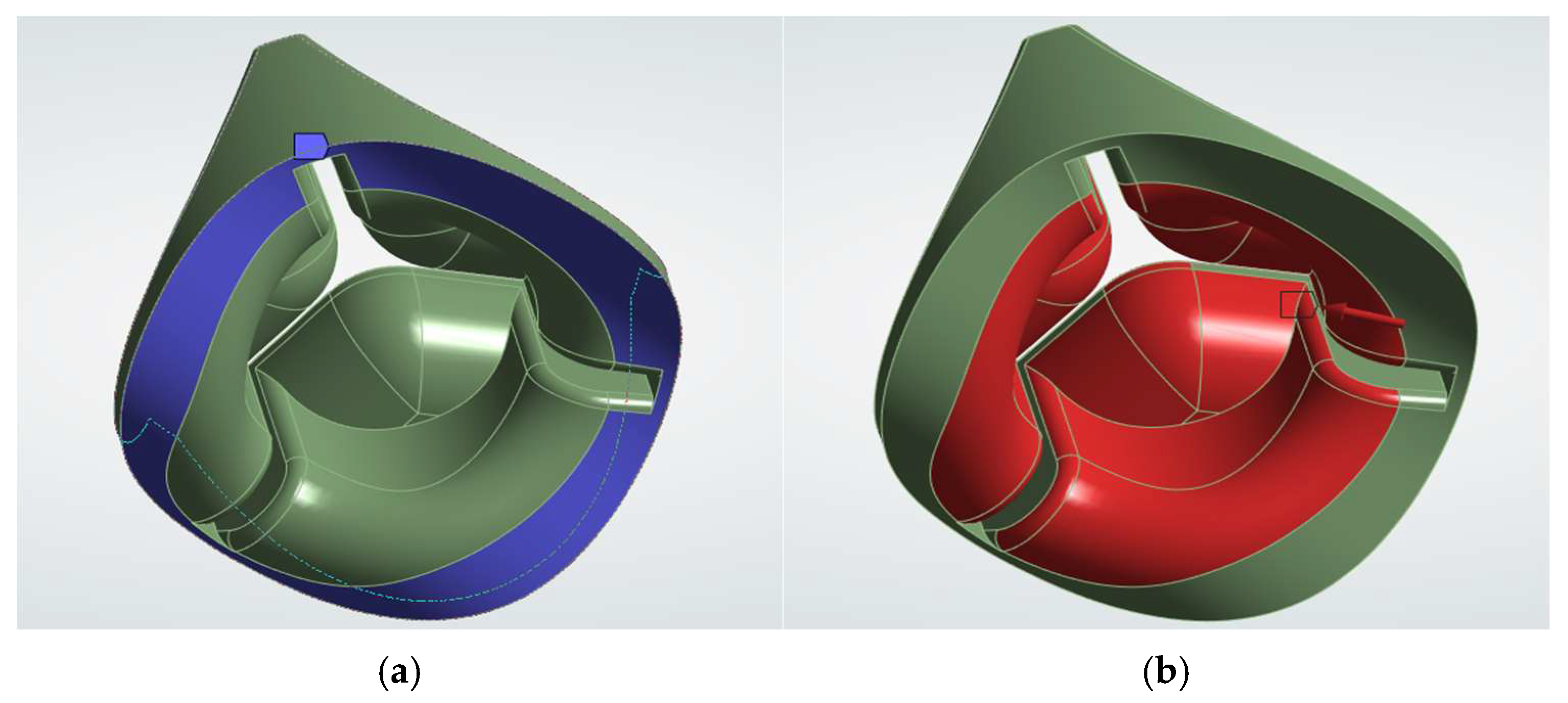
The tricuspid valve geometry used in this study was constructed based on dimensional parameters reported in the literature for prosthetic heart valves [25]. A 23 mm valve configuration was selected as a representative mid-sized prosthetic valve to provide a realistic geometric framework for the computational simulations. The principal geometric parameters included a tissue annulus diameter of 23 mm and a cuff outer diameter of 28 mm. The total valve height was defined as 17 mm, while the aortic protrusion was set to 13 mm. In addition, the mean implanted valve height was assumed to be 16 mm. These geometric dimensions were used to generate the three-dimensional valve model shown in Figure 1 and served as the reference configuration for both the structural and computational fluid dynamics analyses conducted in this study.
These dimensions were used as the reference framework for generating the tricuspid leaflet structure and surrounding annular geometry. The valve leaflets were modeled symmetrically around the annulus, forming three commissures spaced at 120° intervals, consistent with the physiological tricuspid configuration.
The three-dimensional geometry of the valve was created using SolidWorks, 2025 (Dassault Systemes, Waltham, MA, USA) [26]. The completed CAD model was then exported and imported into ANSYS Workbench 2025 R1 for numerical simulations.
To evaluate the structural and hemodynamic behavior of the valve, a computational domain was generated consisting of the valve structure and surrounding fluid regions representing the upstream atrial chamber and downstream ventricular chamber. The structural simulations were performed using ANSYS Mechanical [27], while fluid dynamics simulations were carried out using ANSYS Fluent [28].
This framework allowed independent evaluation of the mechanical deformation of the valve leaflets and the hemodynamic characteristics of blood flow through the valve.
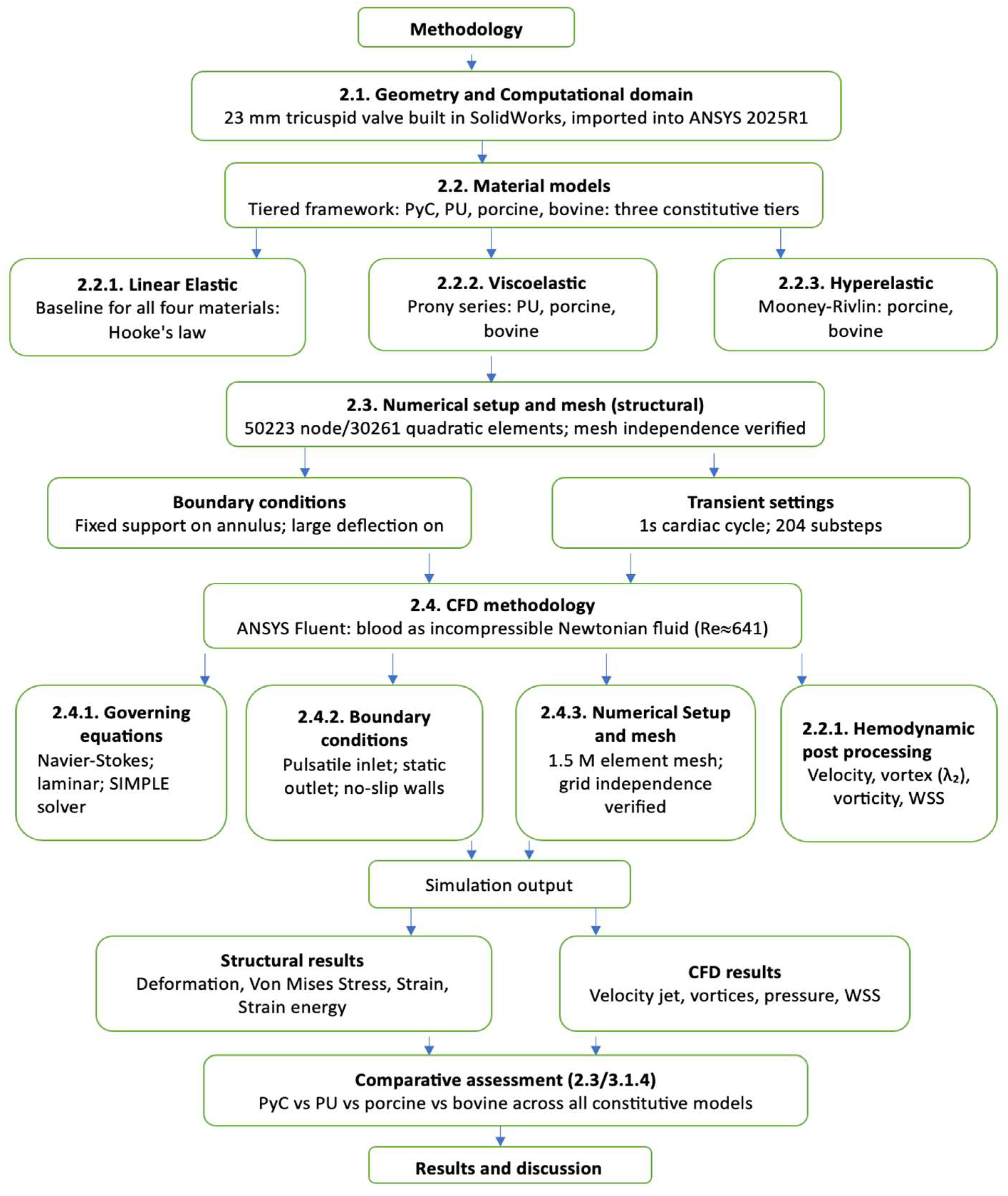
To improve the clarity of the methodology, a flowchart summarizing the main steps of the study has been added in Figure 2. The presentation format was inspired by previously published computational planning workflows [29].

2.2. Material Models

A constitutive model describes how a material deforms under load and should be distinguished from a scalar stress measure such as von Mises stress, which is used only for post-processing and interpretation of the computed stress state. In the present study, different constitutive models were assigned according to the expected physical behavior of each valve material, including pyrolytic carbon, polyurethane, porcine pericardium, and bovine pericardium.
A tiered constitutive framework was adopted to evaluate the influence of stiffness, time-dependency, and nonlinear deformation on tricuspid valve mechanics. Pyrolytic Carbon (PyC) was modeled as an isotropic linear elastic material (E = 29.4 GPa), reflecting its very high stiffness and negligible deformation under physiological loading. Polyurethane (PU) was evaluated using a dual framework using both linear elastic and viscoelastic formulations because polymeric materials can exhibit delayed mechanical response and stress relaxation during cyclic loading. Finally, biological tissues (Porcine and Bovine) were assessed using linear elastic, viscoelastic, and hyperelastic formulations because biological leaflet tissues are compliant, nearly incompressible, and undergo nonlinear large-strain deformation.
To ensure a controlled comparison between constitutive frameworks, the linear elastic tissue properties were selected to represent the small-strain baseline response, whereas the viscoelastic and hyperelastic models were used to capture time-dependent relaxation and nonlinear large-strain behavior, respectively. For the two-parameter Mooney–Rivlin tissues, the equivalent Young’s modulus was estimated from the small-strain form of the constitutive law. The small-strain relationship was calculated according to previously reported Mooney–Rivlin formulations [30,31].
Accordingly, Equation (1) was used:
E = 4(C10 + C01) (1 + ν)
For nearly incompressible materials, this expression is equivalent to
E ≈ 6(C10 + C01) when ν ≈ 0.5.
This approach allows differences in predicted compliance and stress redistribution to be interpreted in relation to constitutive behavior rather than to inconsistent initial stiffness assumptions.

2.2.1. Linear Elastic Model

The linear elastic material model assumes a proportional relationship between stress and strain according to Hooke’s law. This model is commonly used to represent materials that exhibit relatively small deformation and nearly constant stiffness. In the present study, pyrolytic carbon was modeled using a linear elastic formulation due to its high stiffness and negligible nonlinear deformation behavior.
Linear elastic formulations were also applied to polyurethane, porcine pericardium, and bovine pericardium as a simplified baseline model for comparison with more advanced constitutive descriptions. The linear elastic model is defined by two parameters: Young’s modulus and Poisson’s ratio, which describe the stiffness and compressibility of the material.

2.2.2. Viscoelastic Model

Viscoelastic materials exhibit both elastic and time-dependent behavior, meaning that their stress response depends not only on the magnitude of deformation but also on time. A typical feature of viscoelasticity is stress relaxation, in which internal stress decreases when the material is held at a fixed deformation. This behavior is particularly relevant for heart valve materials subjected to repeated pulsatile loading during the cardiac cycle.
In the present study, viscoelasticity was introduced for polyurethane, porcine pericardium, and bovine pericardium because these materials can show delayed mechanical response and damping under cyclic loading. Viscoelastic effects were represented using a one-term Prony series, in which the relaxation modulus decays with time through an exponential term. For the nearly incompressible leaflet materials, relaxation was applied primarily to the shear response, while the volumetric response remained elastic [32].
The viscoelastic parameters assigned to polyurethane were adopted from previously published mechanical characterization studies of biomedical polyurethane elastomers rather than obtained from independent experimental testing in the present work [33]. Likewise, the use of viscoelastic constitutive descriptions for pericardial tissues is supported by prior studies reporting time-dependent stress relaxation in bovine and porcine pericardium [32,34]. Thus, the Prony-series formulation was selected to provide a more realistic representation of transient leaflet behavior than a purely linear elastic approximation [13,33,34,35].

2.2.3. Hyperelastic Model

Biological soft tissues typically undergo large, nonlinear deformations and therefore cannot be accurately described using linear elastic formulations [32]. To capture the nonlinear stress–strain relationship of biological tissues, a hyperelastic material model was employed for porcine pericardium and bovine pericardium. Hyperelastic constitutive models, including Mooney–Rivlin formulations, have been used extensively to represent the large-strain nonlinear behavior of valve leaflet and pericardial biomaterials in computational biomechanics studies [32,35].
In a Mooney–Rivlin hyperelastic model, the material response is defined through a strain-energy density function expressed in terms of deformation invariants and material constants [30,32]. This formulation is particularly suitable for valve leaflet biomaterials because they are compliant, nearly incompressible, and experience nonlinear large-strain deformation during opening and closing. Compared with a linear elastic approximation, the Mooney–Rivlin model provides a more realistic description of stress redistribution in soft biological tissues [35].
By implementing multiple constitutive models for the selected materials, the present study evaluates how different assumptions regarding material behavior influence predicted deformation patterns, stress distribution, and overall leaflet mechanics. In this way, the analysis distinguishes clearly between constitutive laws used to describe material response and scalar stress measures such as von Mises stress used for post-processing.

2.3. Numerical Setup and Mesh Generation (Structural Analysis)

The structural simulations were performed in ANSYS Mechanical (ANSYS 2025 R1). A high-resolution finite element mesh was generated using the Nonlinear Mechanical physics preference, which is suitable for simulations involving nonlinear material behavior and large deformation.
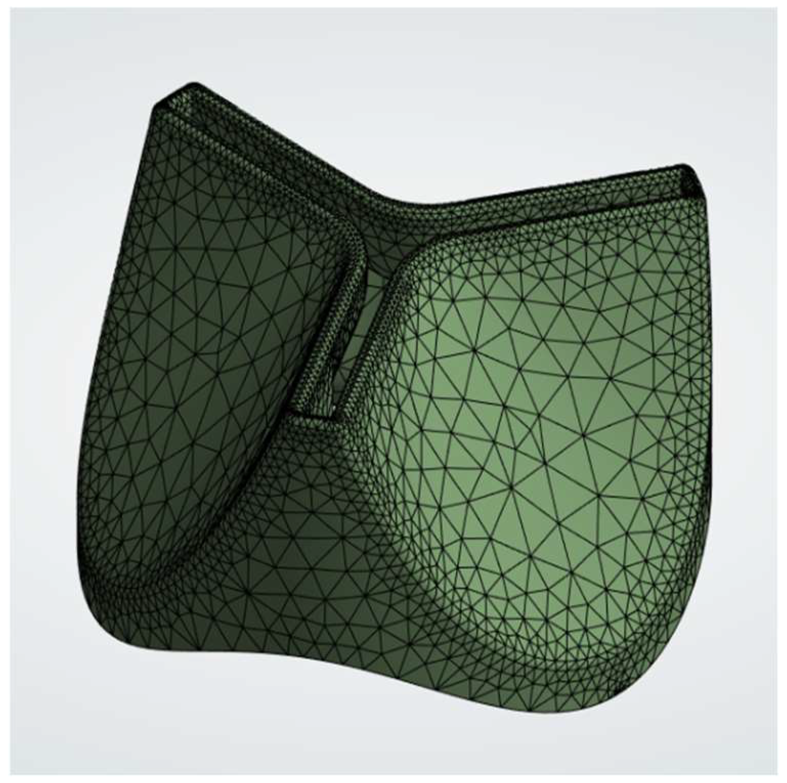
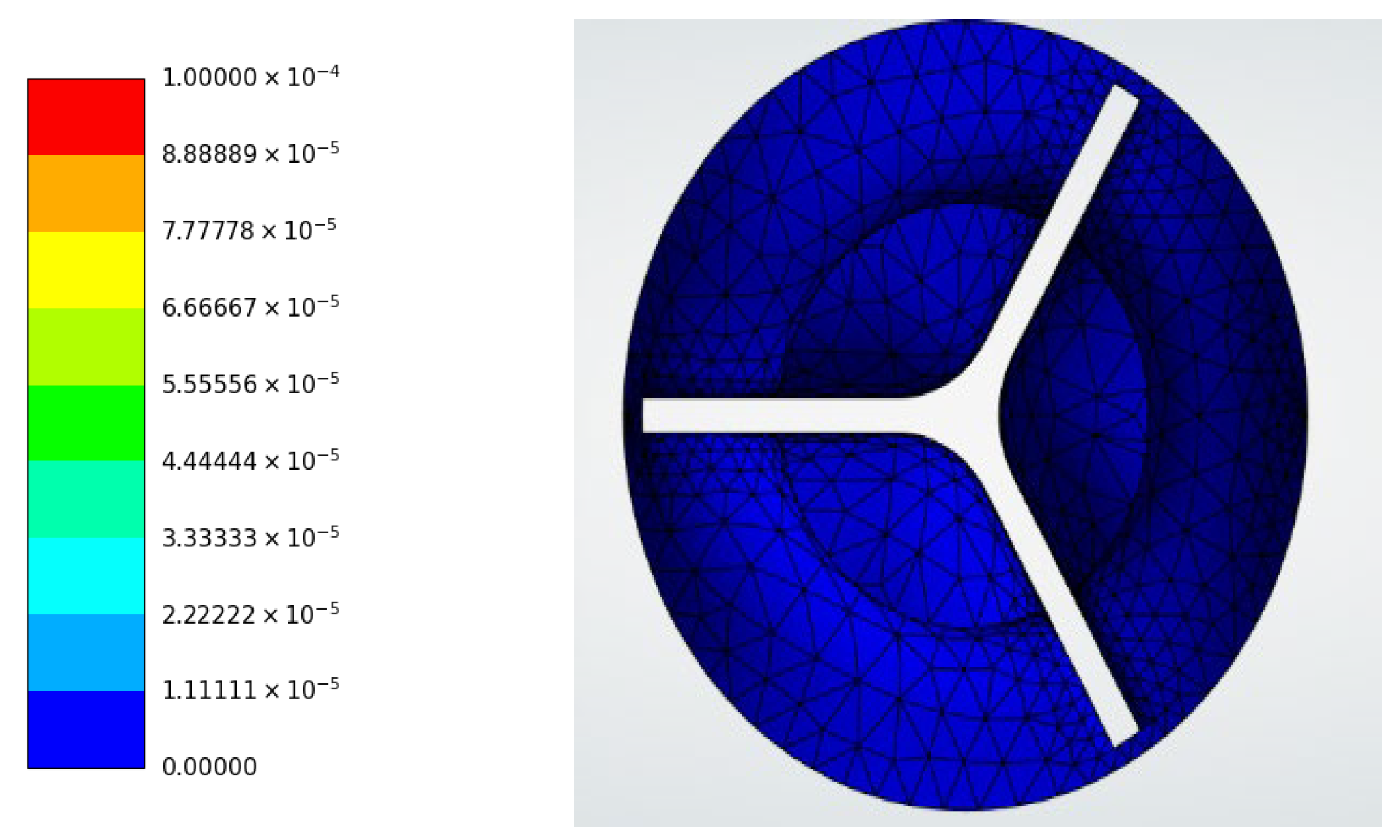
The discretized structural model shown in Figure 3 consisted of 50,223 nodes and 30,261 elements. Quadratic elements were used throughout the mesh to improve numerical accuracy, particularly in regions of high stress concentration near the leaflet attachment and commissural regions.
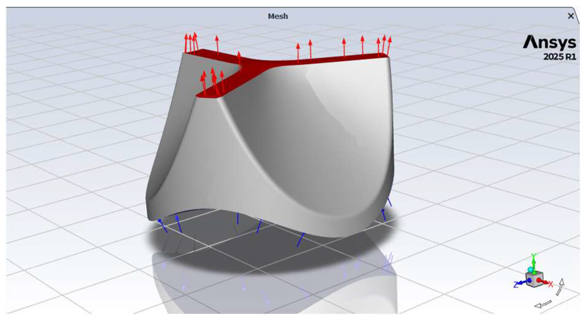
Because several of the materials investigated exhibit nonlinear mechanical behavior, large deflection effects were enabled during the structural analysis. The transient structural response of the valve was simulated over a 1.0 s cardiac cycle, which represents a full physiological loading period. The solution was computed using 204 substeps, resulting in a total of 387 solver iterations, ensuring stable convergence during both the loading and unloading phases of the cycle. The boundary conditions used for the structural analysis of the tricuspid leaflet are illustrated in Figure 4. The leaflet attachment region was defined as a fixed support to represent anchoring at the annulus, while a uniform pressure load of 500 Pa (approximately 3.75 mmHg) was applied normal to the leaflet surface. This loading magnitude was selected from literature-reported low right-sided transvalvular conditions and was used in the present study as a simplified representative physiological load for comparative structural assessment of the different material models, rather than as a patient-specific transvalvular pressure. This value is consistent with the low-pressure right-sided environment of the tricuspid valve, where normally functioning tricuspid prostheses generally exhibit mean gradients below 6 mmHg [36,37,38].
A mesh independence study was performed to ensure numerical stability; increasing the element count beyond 30,261 resulted in a 3% change in peak von-Mises stress, confirming that the selected discretization was sufficient for the transient gradients observed.

2.4. Computational Fluid Dynamics (CFD) Methodology

2.4.1. Governing Equations and Flow Regime

The hemodynamic performance of the tricuspid valve was evaluated by solving the Navier–Stokes equations, which describe the conservation of mass and momentum for fluid flow [39]. Blood was modeled as an incompressible Newtonian fluid with a density of 1060 kg/m3 and a dynamic viscosity of 0.0035 Pa·s, which are commonly used values in cardiovascular flow simulations. The flow was modeled as laminar, given the low Reynolds number (Re approx. 641) calculated at the peak velocity of 0.092 m/s. The Pressure-Based solver in ANSYS Fluent was utilized with the SIMPLE (Semi-Implicit Method for Pressure-Linked Equations) scheme for pressure-velocity coupling, and second-order upwind discretization was used for momentum equations to reduce numerical diffusion.
Under physiological conditions, blood flow through the tricuspid valve occurs at relatively moderate velocities, allowing the flow to be reasonably approximated as laminar. The analysis focused on the formation of the forward flow jet through the valve orifice and the development of localized recirculation zones downstream of the valve leaflets.

2.4.2. Boundary Conditions and Pulsatile Flow

To represent physiological cardiac conditions, the following boundary conditions as shown in Figure 5 were applied to the computational domain.
  • Inlet:
A pulsatile velocity profile was prescribed at the inlet to simulate the time-dependent blood flow associated with the diastolic filling phase of the cardiac cycle. This time-varying velocity distribution drives the formation of a central jet through the valve opening.
  • Outlet:
A static pressure boundary condition was applied at the outlet of the domain. This allowed the solver to calculate the pressure distribution and the resulting pressure gradient across the valve.
  • Walls:
All chamber walls and valve surfaces were assigned a no-slip boundary condition, ensuring that the fluid velocity approaches zero at the solid–fluid interface.
  • Valve Configuration:
For the CFD simulations, the valve was modeled as a rigid structure fixed in its fully open position. This configuration allows for evaluation of the peak hemodynamic effects of valve geometry on blood flow.

2.4.3. Numerical Setup and Mesh

The CFD simulations were performed using ANSYS Fluent (ANSYS 2025 R1). A high-resolution computational mesh was generated to accurately capture the strong velocity gradients near the leaflet edges and within the valve orifice region. A Grid Independence Study was performed to ensure the reliability of the hemodynamic results. This numerical approach aligns with contemporary high-resolution studies validating transient flow gradients in prosthetic valves [23]. The fluid domain was discretized using three successive mesh densities (0.8 M, 1.5 M, and 2.2 M elements). The variation in peak velocity at the orifice was found to be less than 0.8% between the medium and fine meshes; therefore, the 1.5 M element mesh was selected for the final analysis to balance computational efficiency and numerical accuracy.
The governing equations were solved using the pressure-based solver, and convergence of the numerical solution was monitored through the reduction in residuals for the continuity and momentum equations. The simulations were considered converged once the residuals reached standard tolerance levels and the monitored flow variables stabilized.

2.4.4. Hemodynamic Post-Processing

Several hemodynamic parameters were evaluated to assess the flow characteristics through the tricuspid valve.
Velocity Jet Characterization:
Velocity contour plots and streamline visualizations were used to analyze the formation and propagation of the central flow jet through the valve.
Vortex Identification:
The Lambda-2 criterion was employed to identify coherent vortex structures and recirculation regions in the downstream flow field.
Vorticity:
The magnitude of the velocity curl was calculated to quantify the rotational strength of the flow, particularly near the leaflet edges where geometric discontinuities exist.
Wall Shear Stress (WSS):
Both instantaneous and mean wall shear stress distributions were computed on the valve surfaces. WSS is an important parameter for evaluating potential blood cell damage, platelet activation, and overall hemocompatibility of prosthetic valve designs.

3. Results

3.1. Structural Analysis

The structural response of the tricuspid valve was evaluated through transient finite element simulations for nine material configurations representing rigid, polymeric, and biological valve materials. The resulting deformation, stress distribution, strain, and strain energy were analyzed to assess the influence of material stiffness and constitutive modeling assumptions on valve mechanics. The quantitative maximum values extracted from the simulations are summarized in Table 1.
The quantitative results in Table 1 indicate a clear hierarchy of mechanical response across the investigated material classes. Pyrolytic carbon remained functionally rigid, with deformation and strain several orders of magnitude below those of the tissue-based models. Polyurethane showed intermediate behavior, combining moderate deformation with substantially reduced stress under viscoelastic modeling. The porcine and bovine tissues exhibited the highest strain and strain-energy storage, indicating greater compliance and mechanical damping capacity. These trends suggest that the principal trade-off is between structural rigidity and physiological compliance: rigid materials minimize deformation but store little strain energy, whereas compliant biological tissues deform more but redistribute stress more effectively.

3.1.1. Deformation Response

The deformation behavior of the valve leaflets was strongly dependent on the stiffness and constitutive model of the material.
Linear Elastic Materials
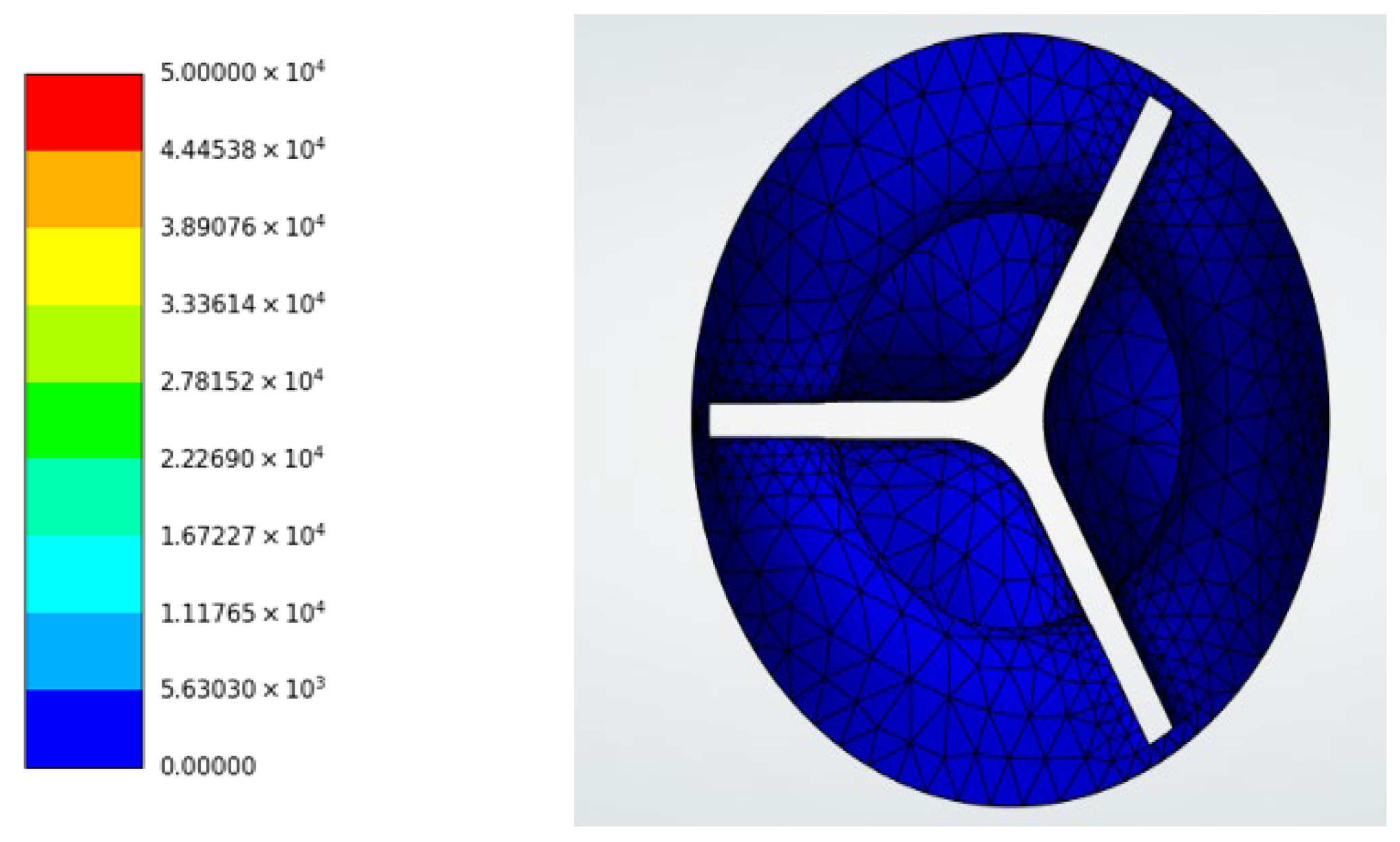
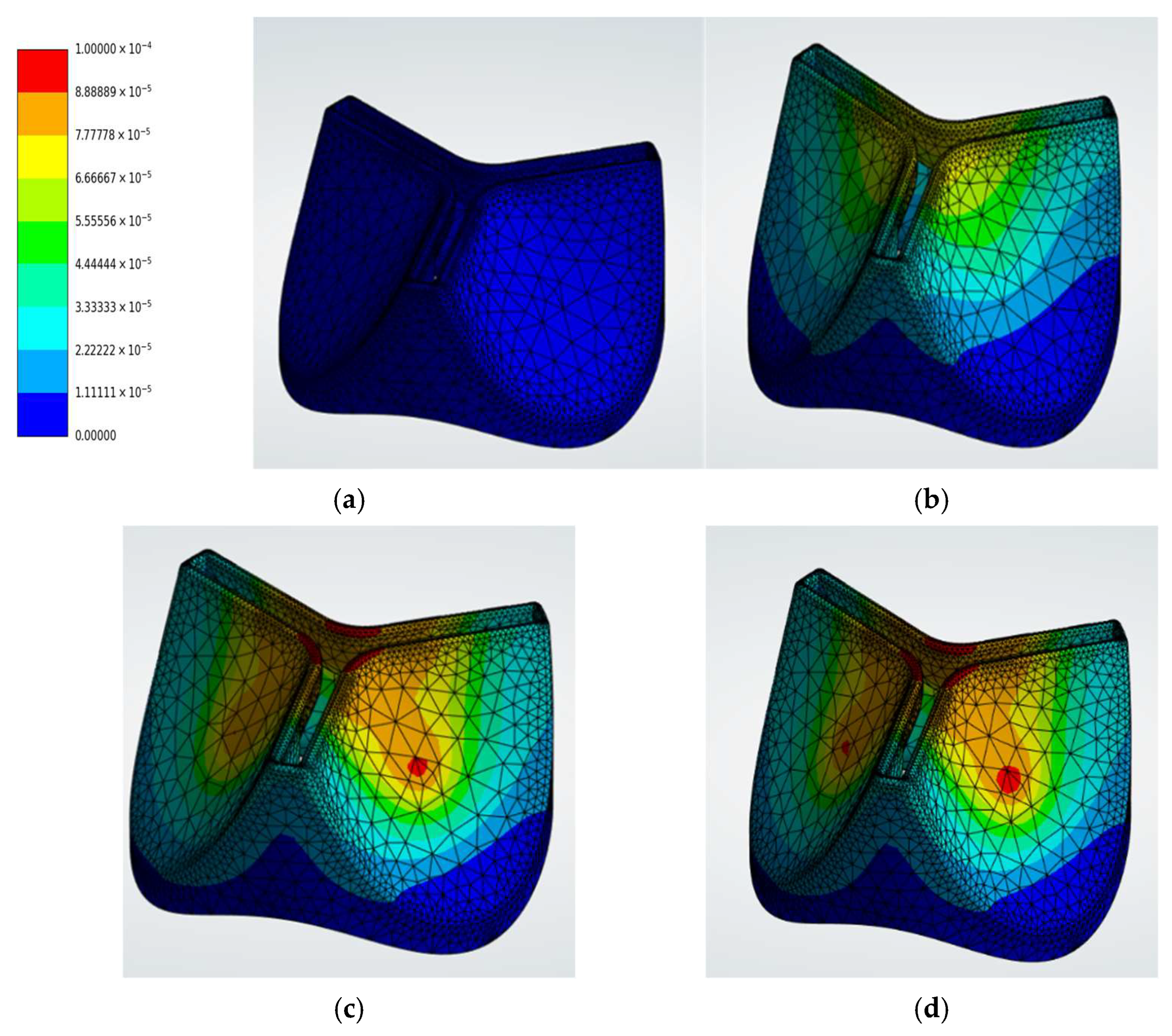
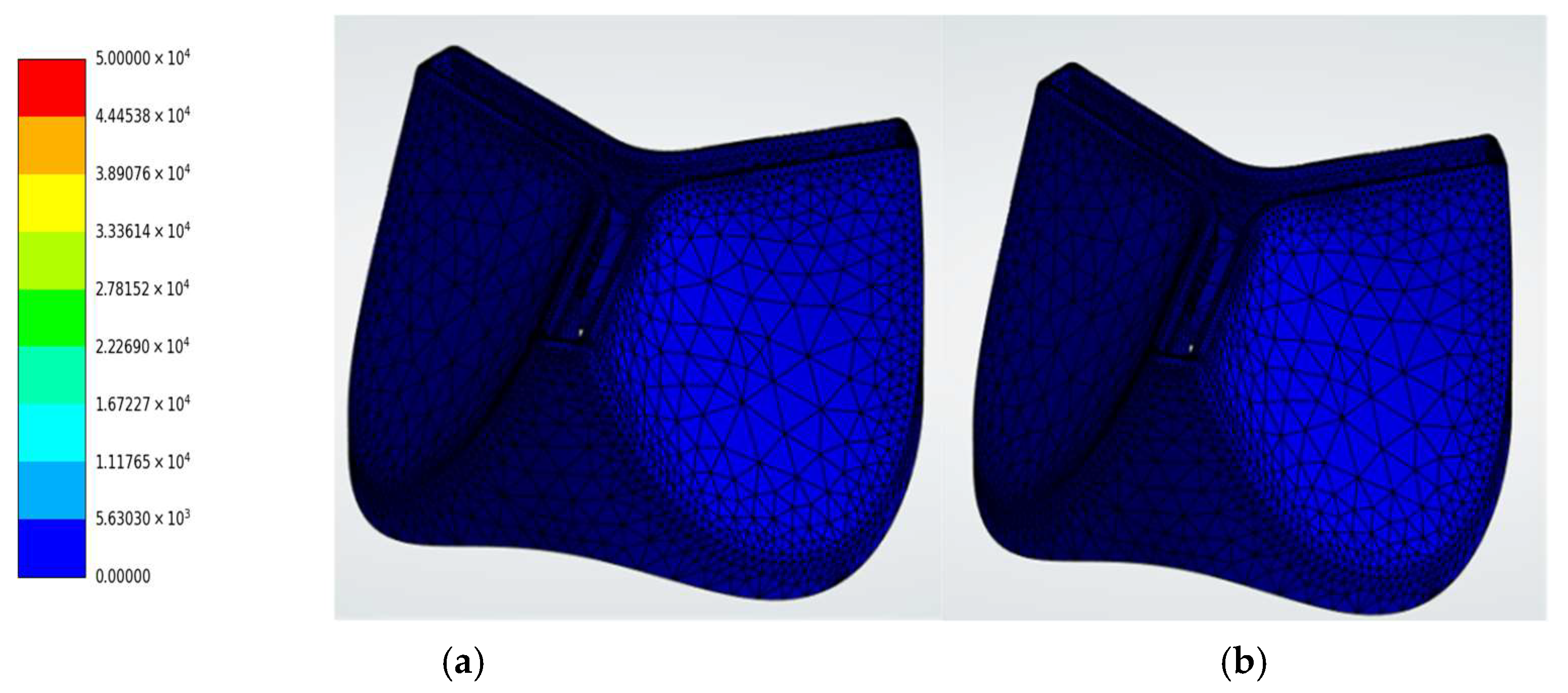
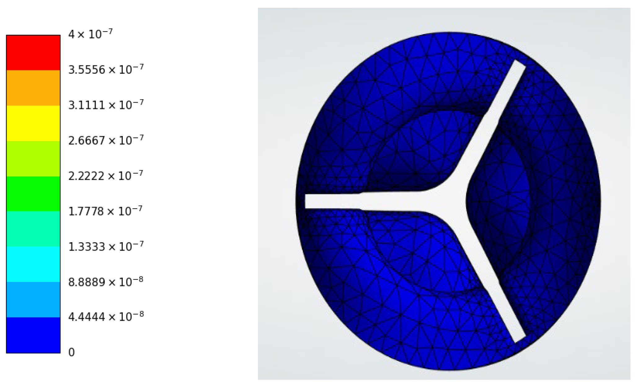
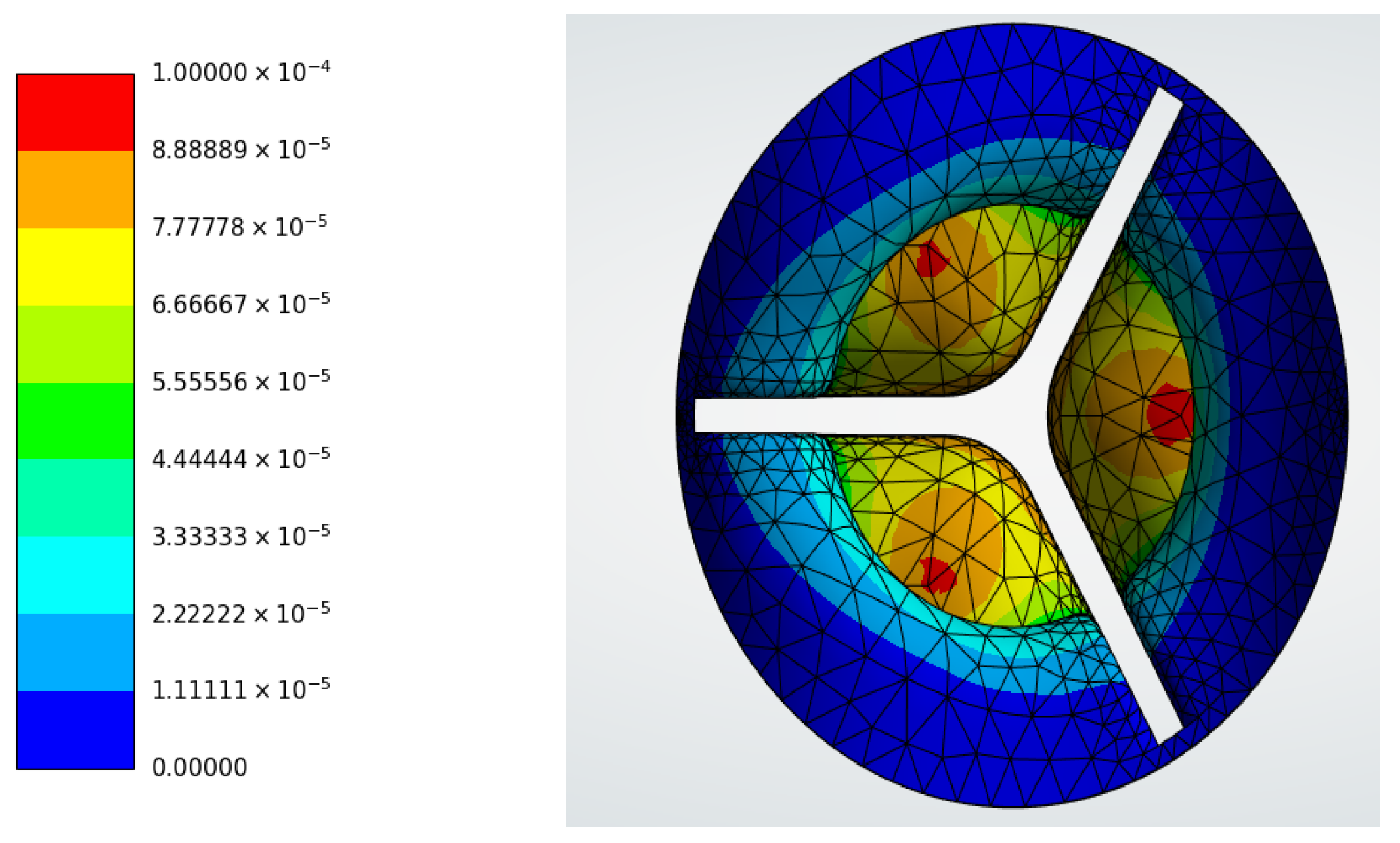
The deformation contours for the linear elastic material models are shown in Figure 6. Among these materials, pyrolytic carbon (Figure 6a) exhibited the smallest deformation of 1.7166 × 10⁻⁸ m, reflecting its extremely high stiffness and minimal flexibility. In contrast, polyurethane (Figure 6b) showed moderate deformation of 7.6515 × 10⁻⁵ m, indicating greater compliance compared with pyrolytic carbon.
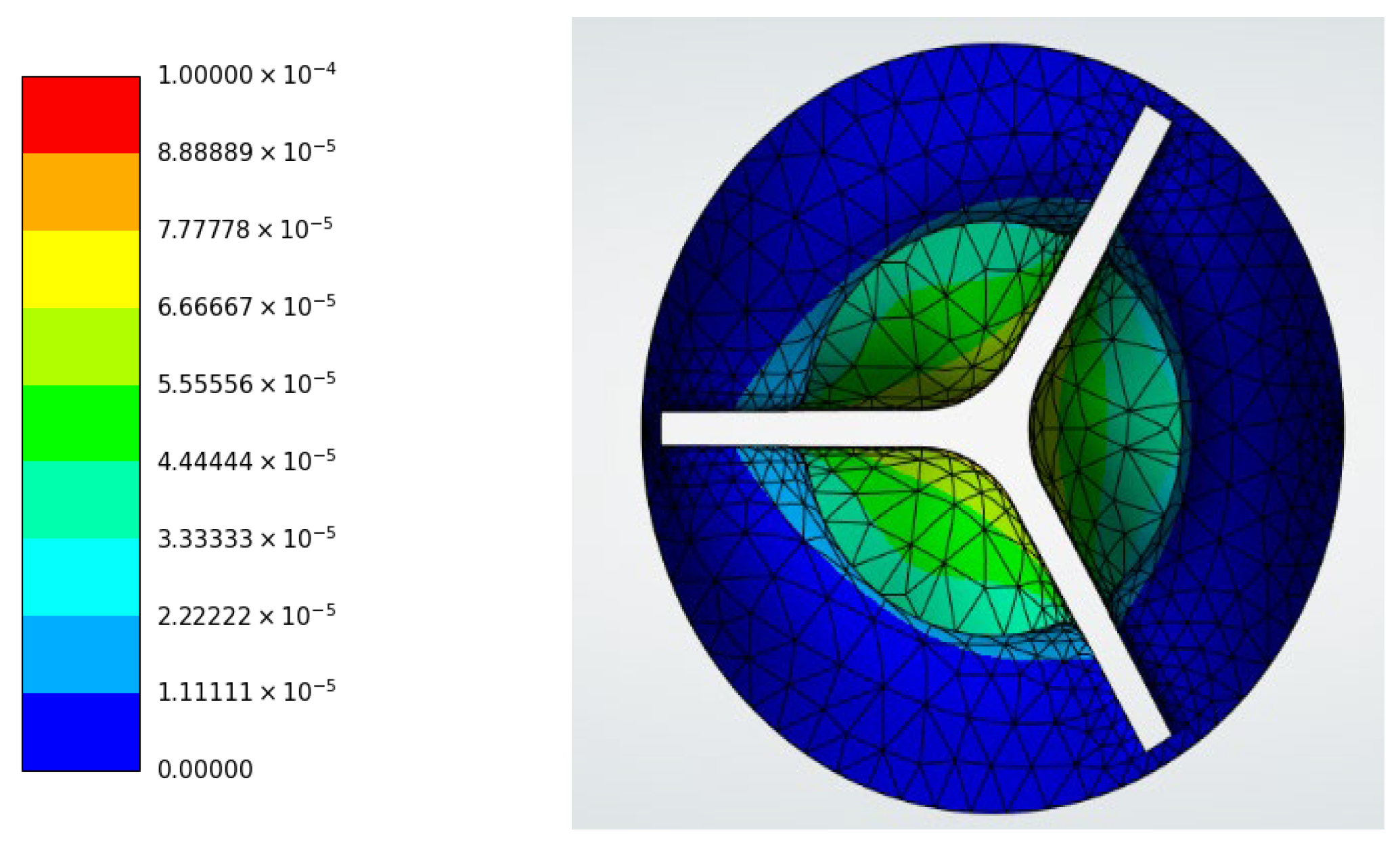
The biological tissues displayed slightly larger deformation magnitudes within the linear elastic framework. The porcine linear elastic model (Figure 6c) reached a maximum deformation of 9.3878 × 10⁻⁵ m, while the bovine linear elastic model (Figure 6d) reached 9.6104 × 10⁻⁵ m, which was the largest deformation among the linear elastic materials. As illustrated in Figure 6c,d, deformation was concentrated primarily near the leaflet free edges and commissural regions, where bending deformation is dominant.
  • Viscoelastic Materials
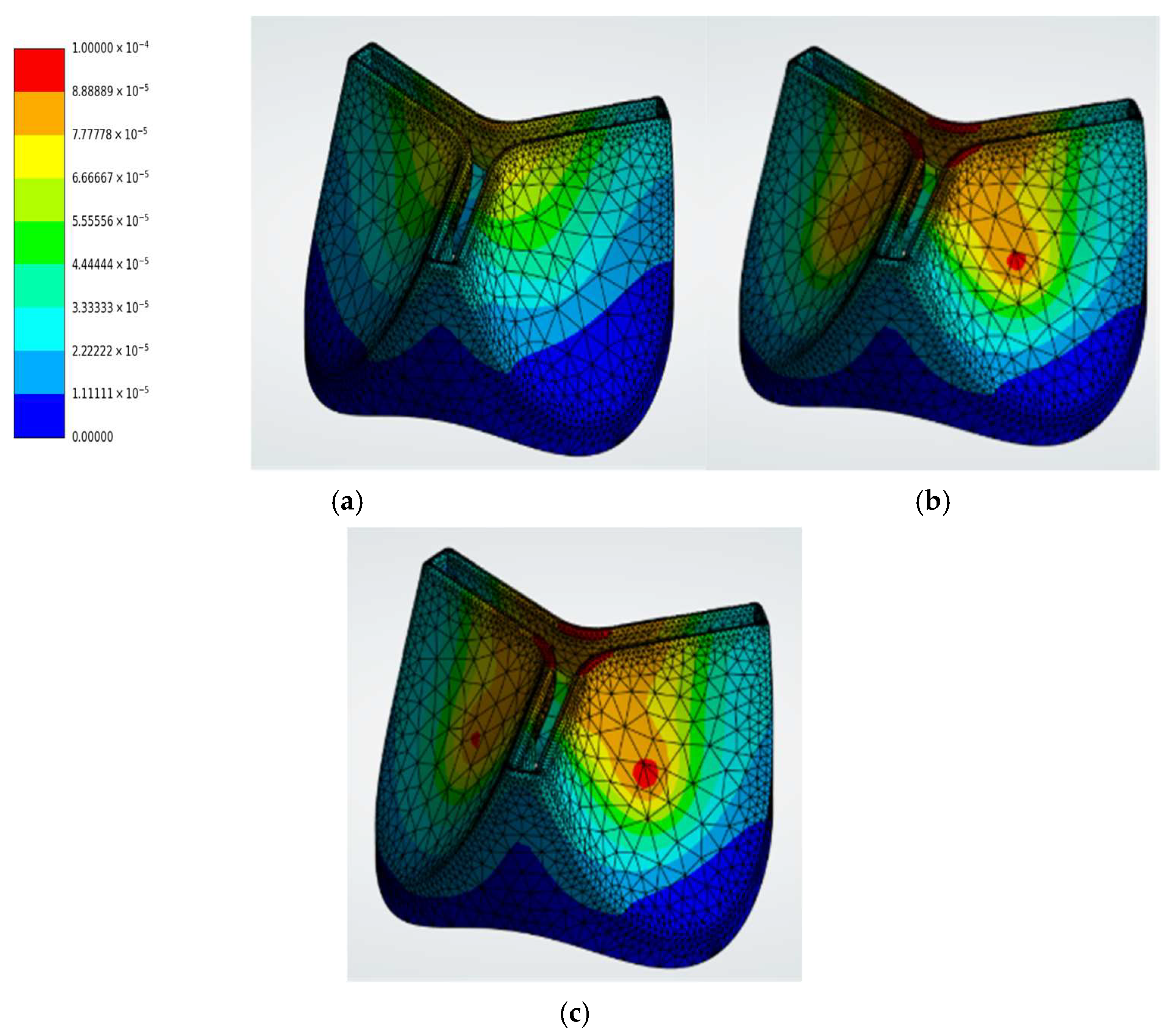
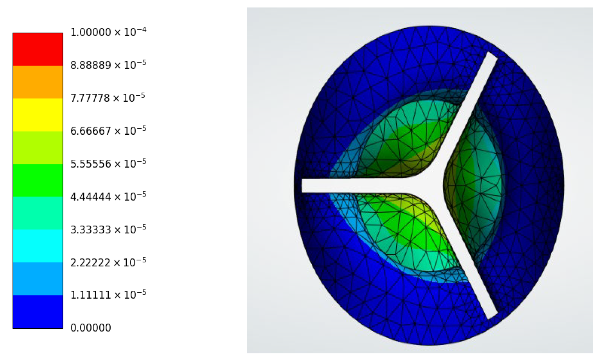
The deformation patterns for the viscoelastic materials are shown in Figure 7. Incorporating viscoelasticity introduced time-dependent deformation behavior. Polyurethane (Figure 7a) exhibited a slightly larger deformation of 7.8948 × 10⁻⁵ m, compared with the linear elastic case. The porcine viscoelastic model (Figure 7b) showed a maximum deformation of 9.3311 × 10⁻⁵ m, whereas the bovine viscoelastic model (Figure 7c) exhibited a maximum deformation of 9.5439 × 10⁻⁵ m. The deformation contours in Figure 7 demonstrate displacement along the leaflet surfaces due to the delayed elastic response characteristic of viscoelastic materials.
Hyperelastic Materials
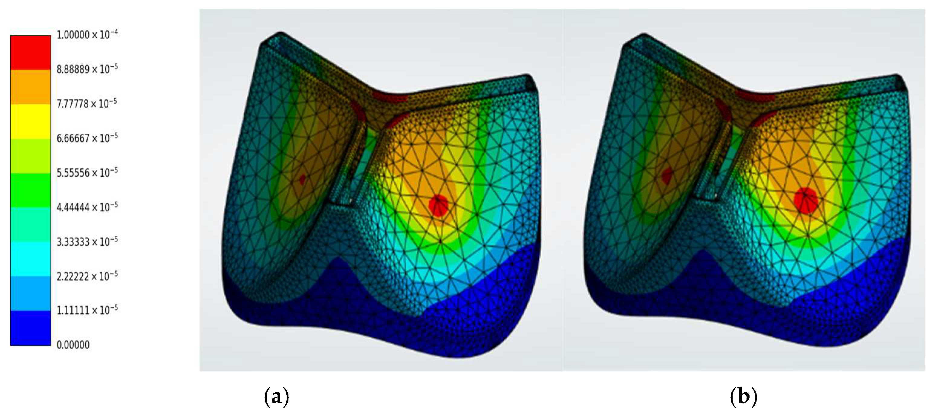
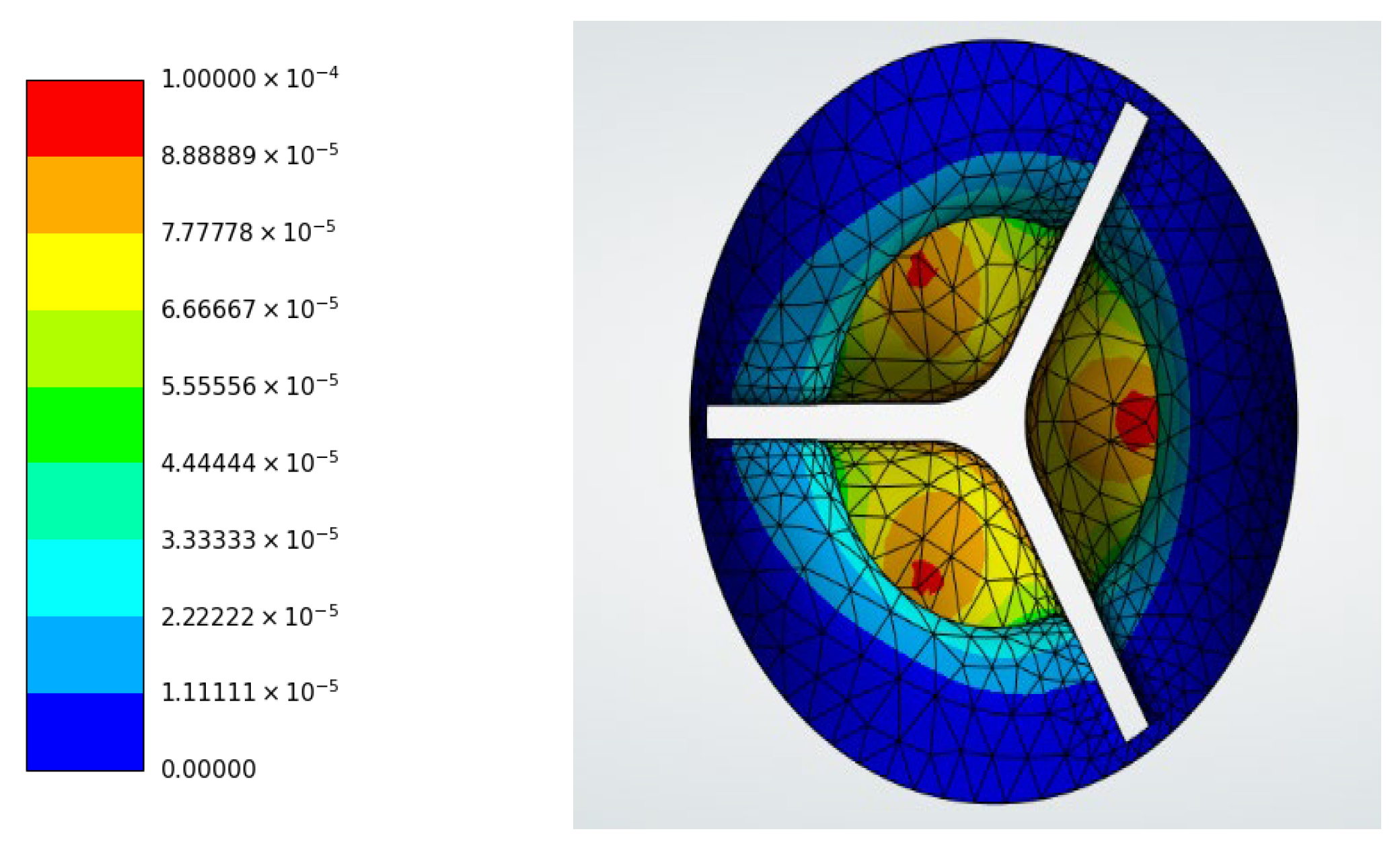
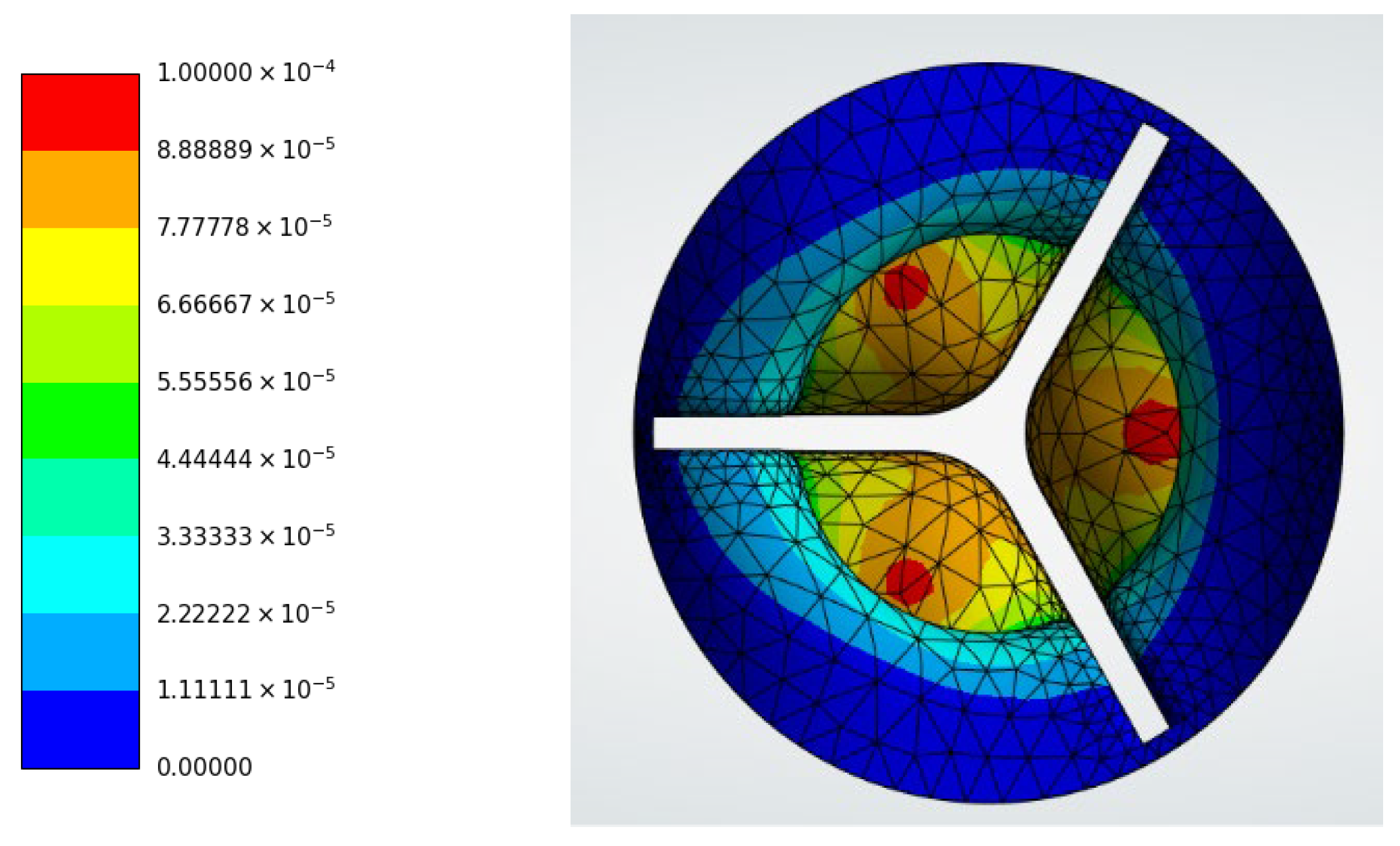
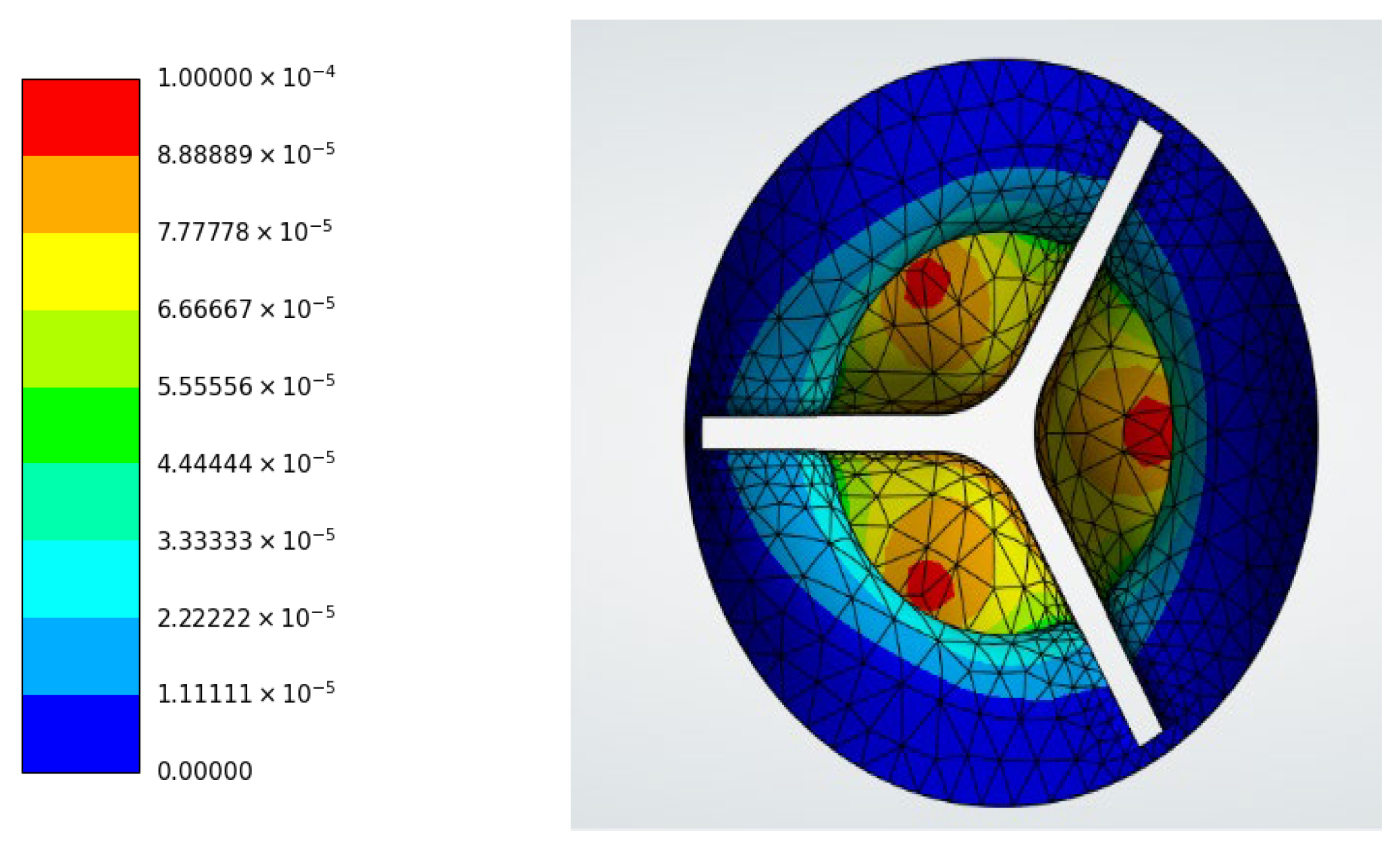
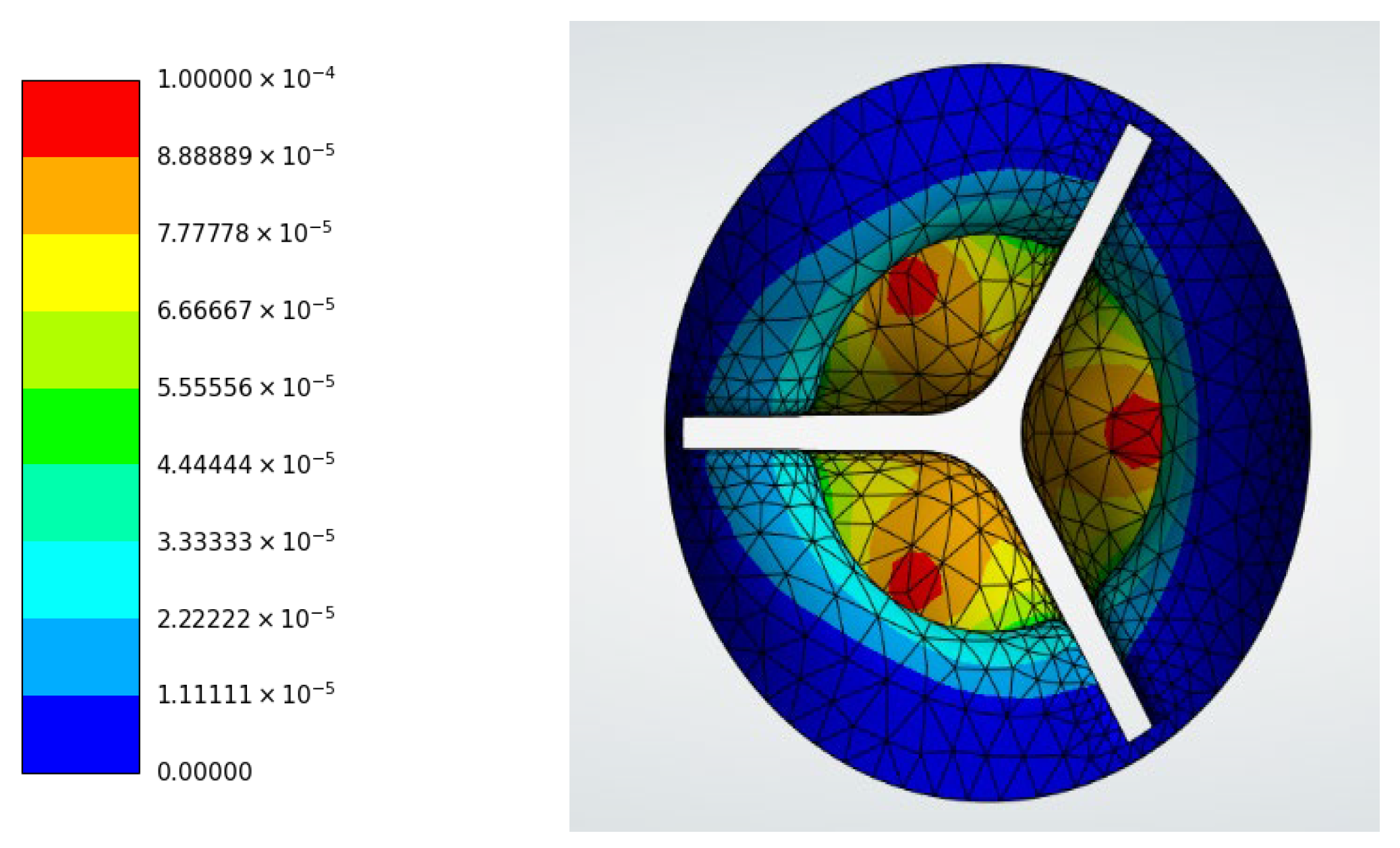
The hyperelastic tissue models shown in Figure 8 captured nonlinear large-strain behavior. The porcine hyperelastic model (Figure 8a) exhibited a deformation of 9.4845 × 10⁻⁵ m, while the bovine hyperelastic model reached 9.6837 × 10⁻⁵ m. Compared with the linear elastic models, the hyperelastic formulations produced comparable deformation magnitudes but smoother deformation gradients across the leaflet surface, particularly near the central leaflet region, as visible in Figure 8a,b.

3.1.2. Stress Distribution

The stress distribution within the valve structure varied considerably depending on the material model.
Linear Elastic Materials
Von-Mises Stress
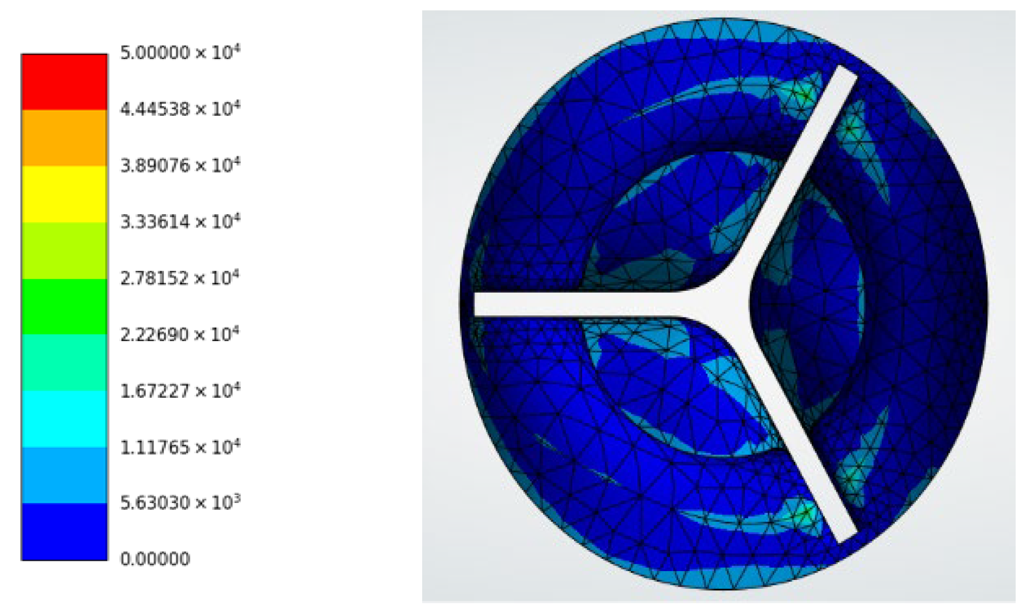
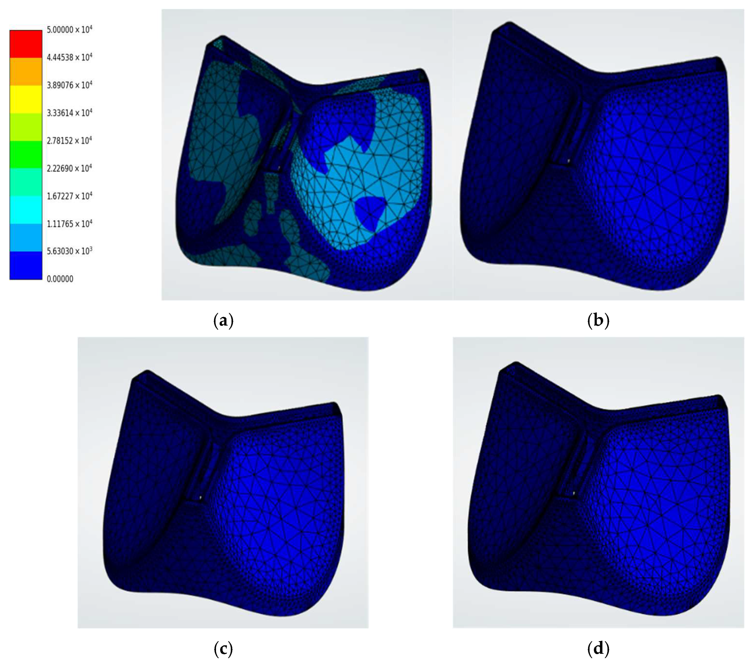
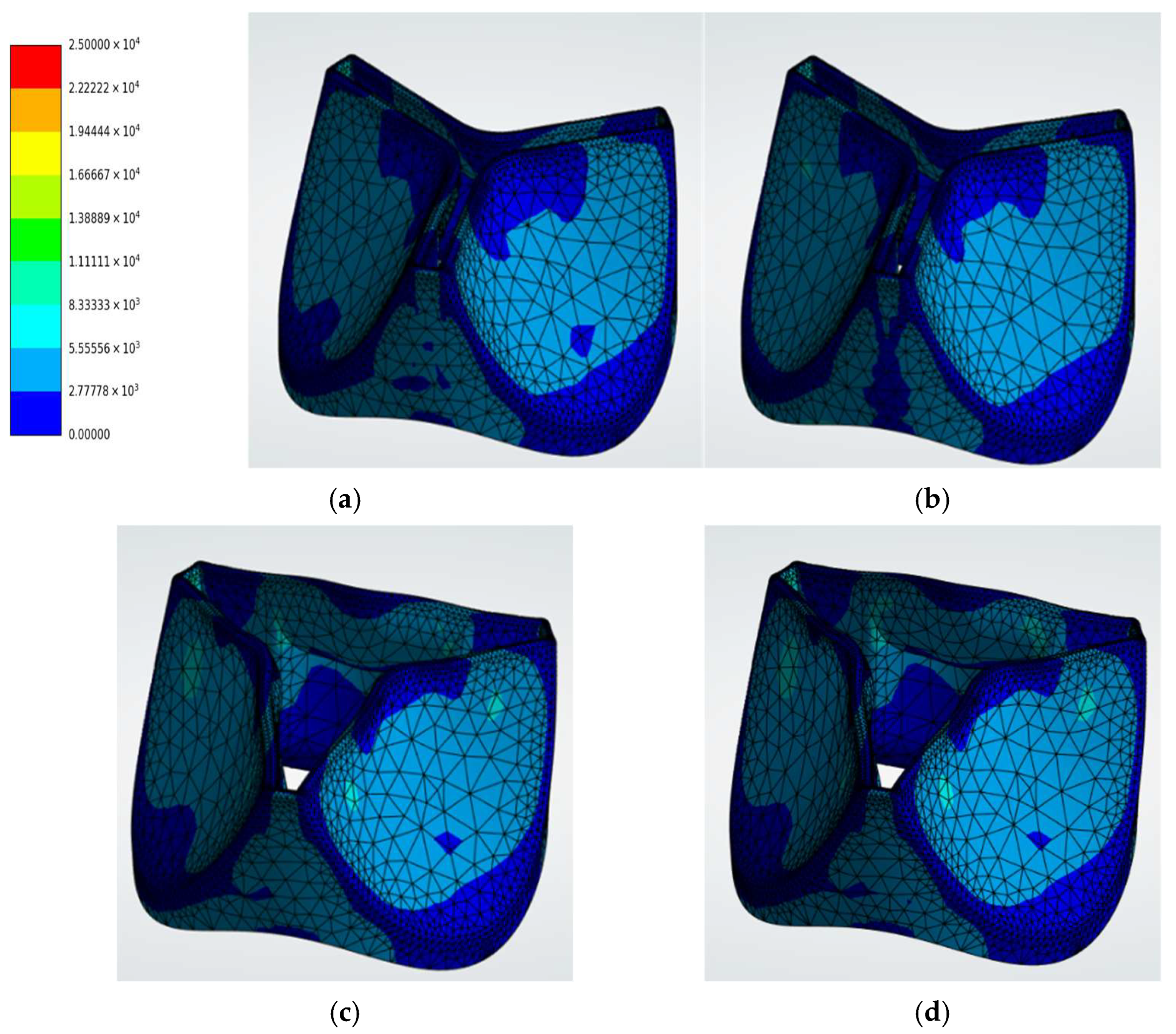
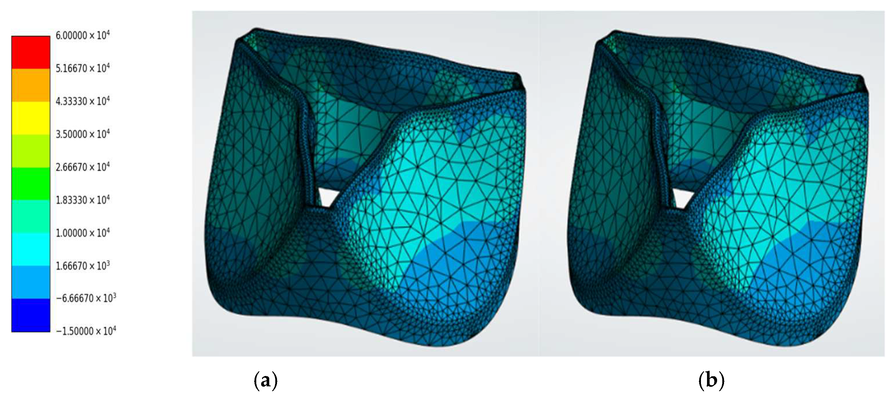
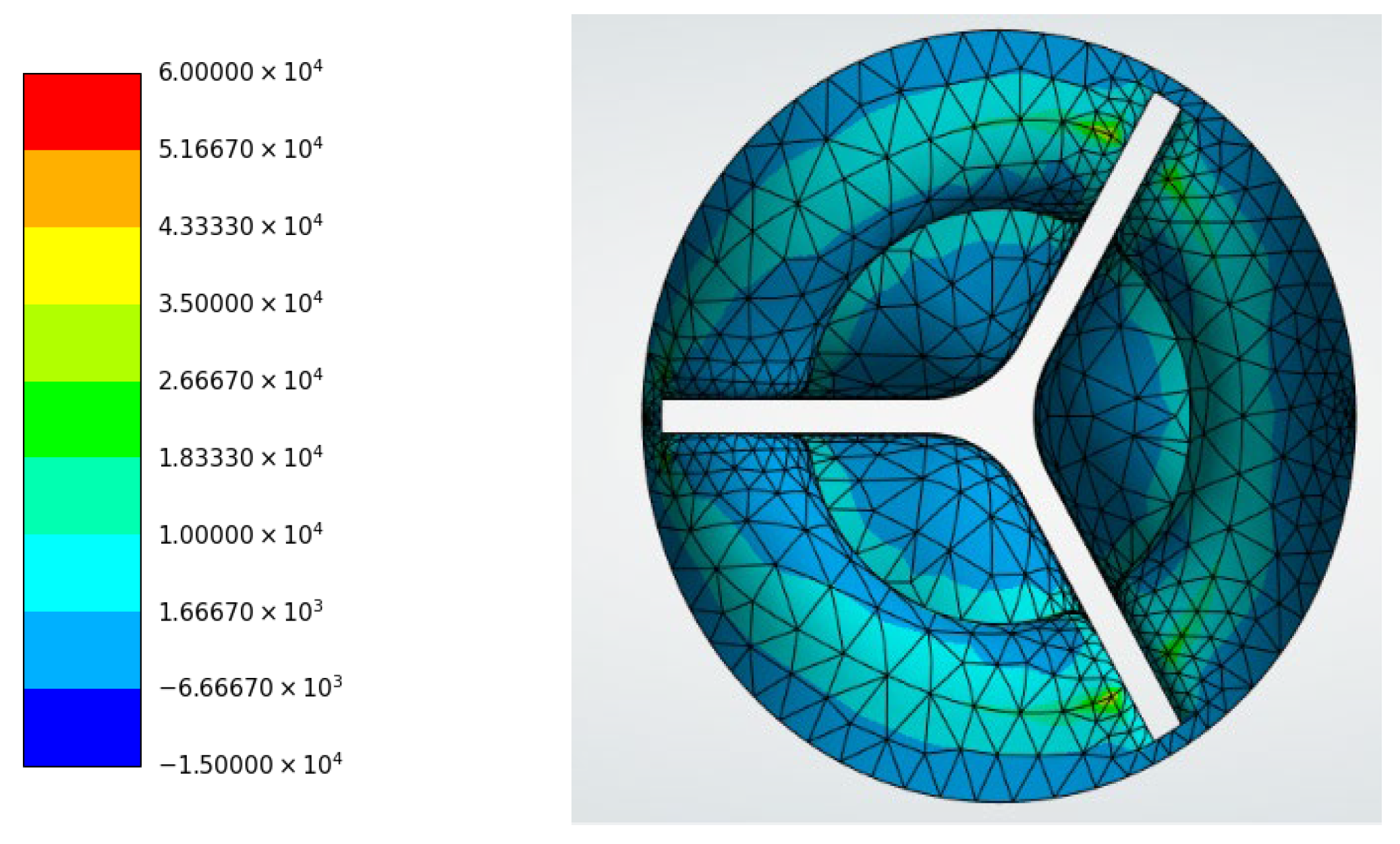
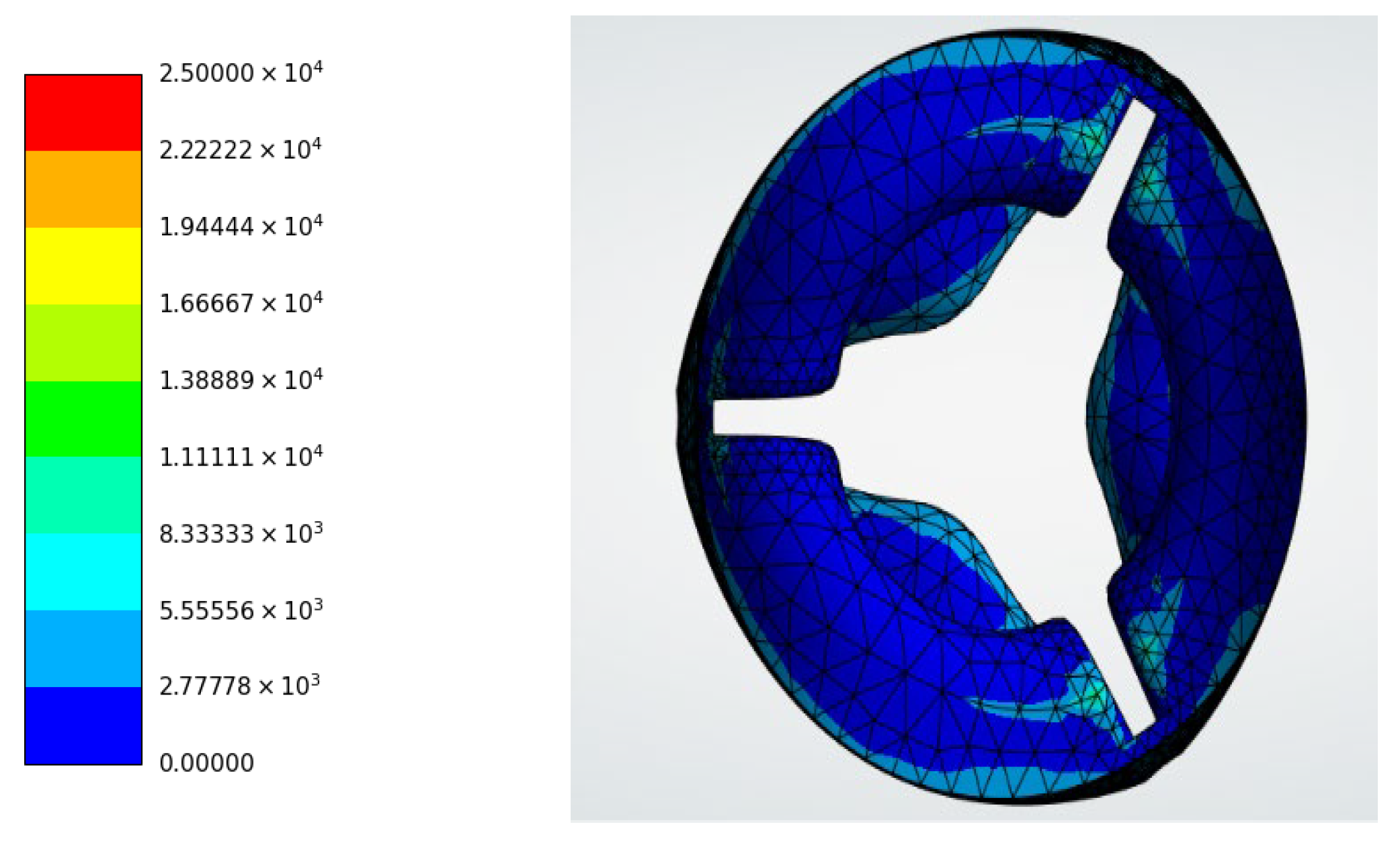
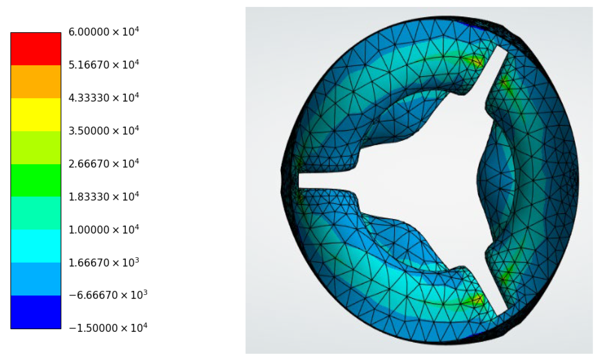
The von Mises stress contours for the linear elastic materials are shown in Figure 9. Pyrolytic carbon (Figure 9a) experienced a maximum von Mises stress of 3.4356 × 10⁴ Pa, while polyurethane (Figure 9b) exhibited the highest stress among the linear elastic materials at 4.0839 × 10⁴ Pa. The biological tissues showed lower stress magnitudes, with porcine tissue (Figure 9c) reaching 2.6842 × 10⁴ Pa and bovine tissue (Figure 9d) reaching 2.7017 × 10⁴ Pa. As illustrated in Figure 9, stress concentrations were primarily located near the leaflet attachment regions and commissures.
Maximum Principal Stress
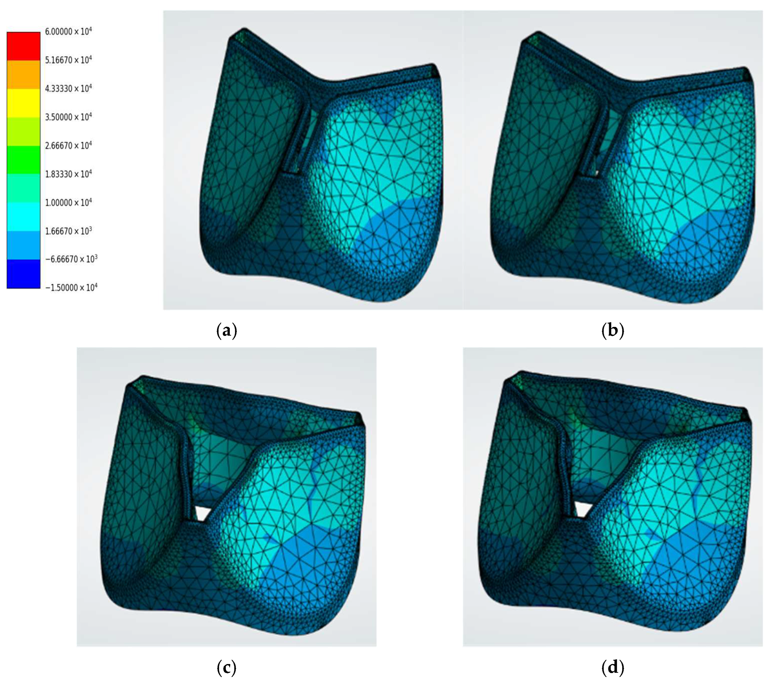
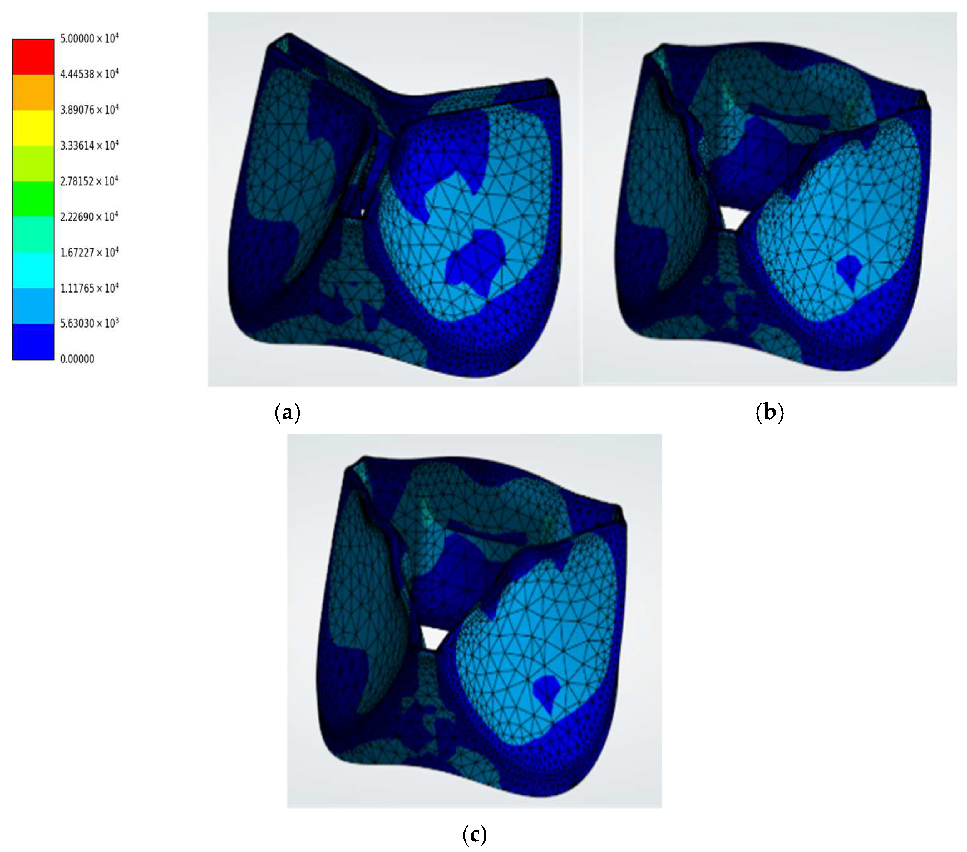
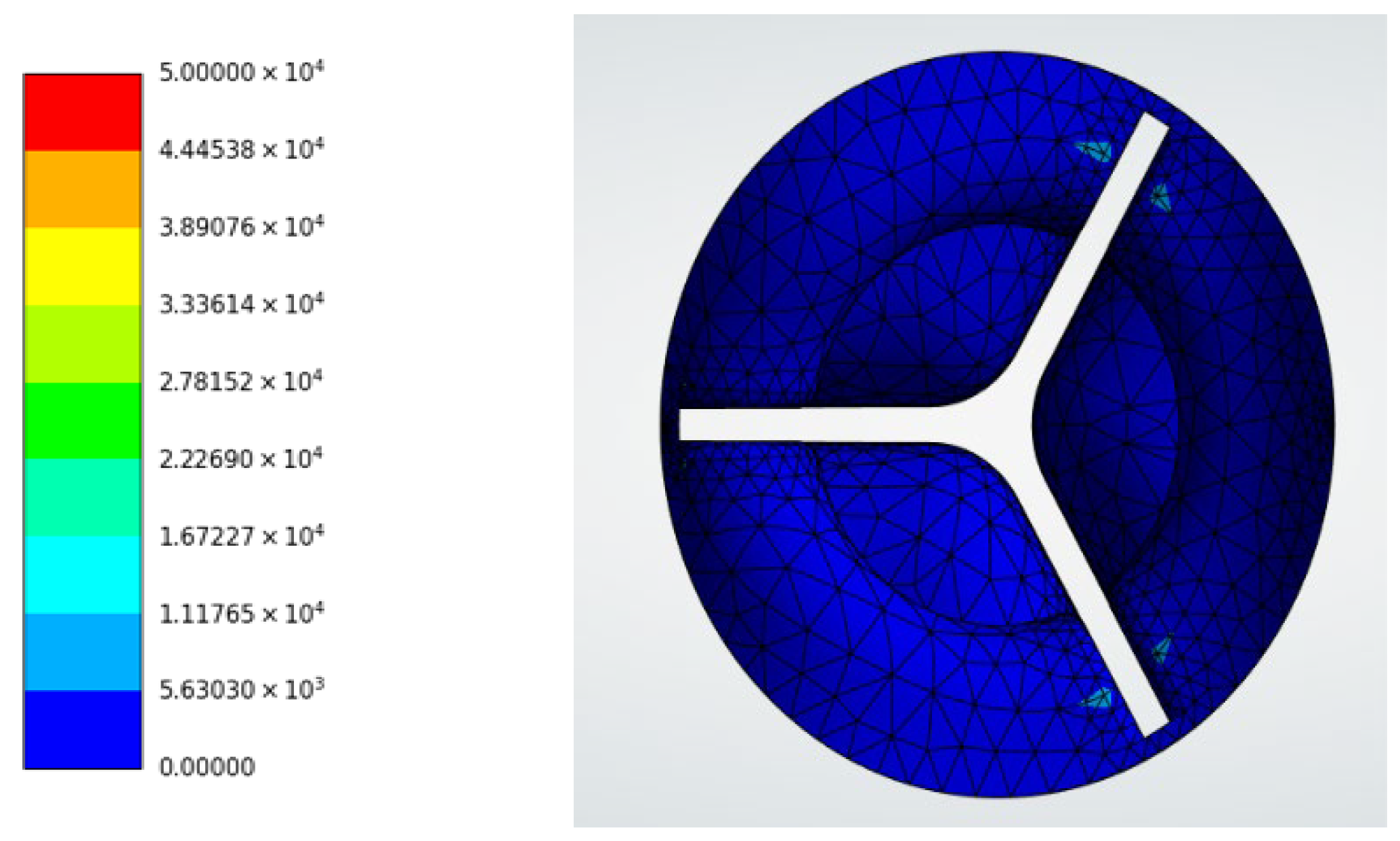
The maximum principal stress distributions presented in Figure 10 reveal the regions subjected to tensile loading. The maximum principal stress reached 5.3069 × 10⁴ Pa for pyrolytic carbon (Figure 10a), while polyurethane (Figure 10b) exhibited 4.9016 × 10⁴ Pa. The porcine (Figure 10c) and bovine (Figure 10d) models showed tensile stress magnitudes of 4.9068 × 10⁴ Pa and 5.6877 × 10⁴ Pa, respectively. These stresses were concentrated along the leaflet edges and near the commissural junctions.
Maximum Shear Stress
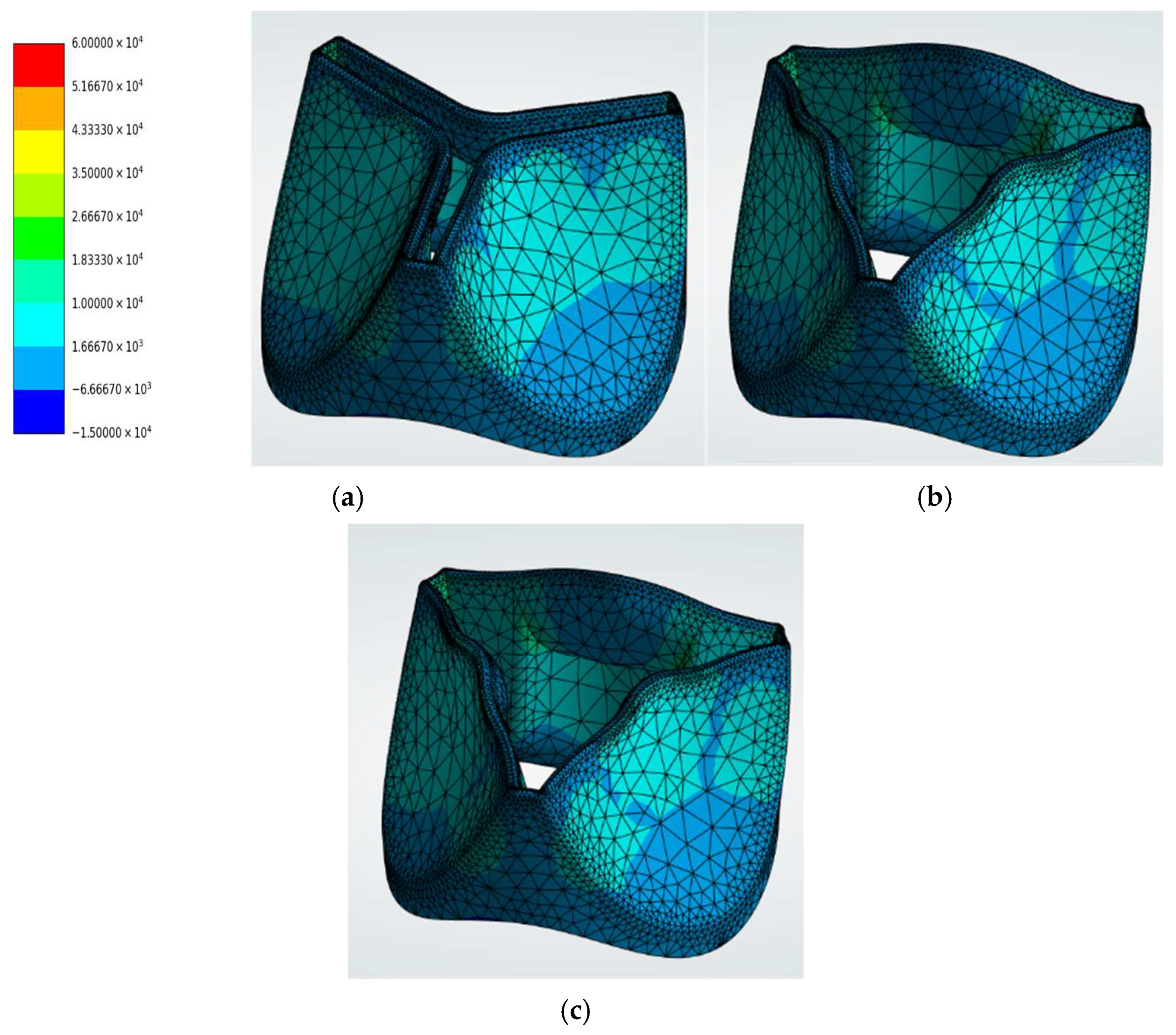
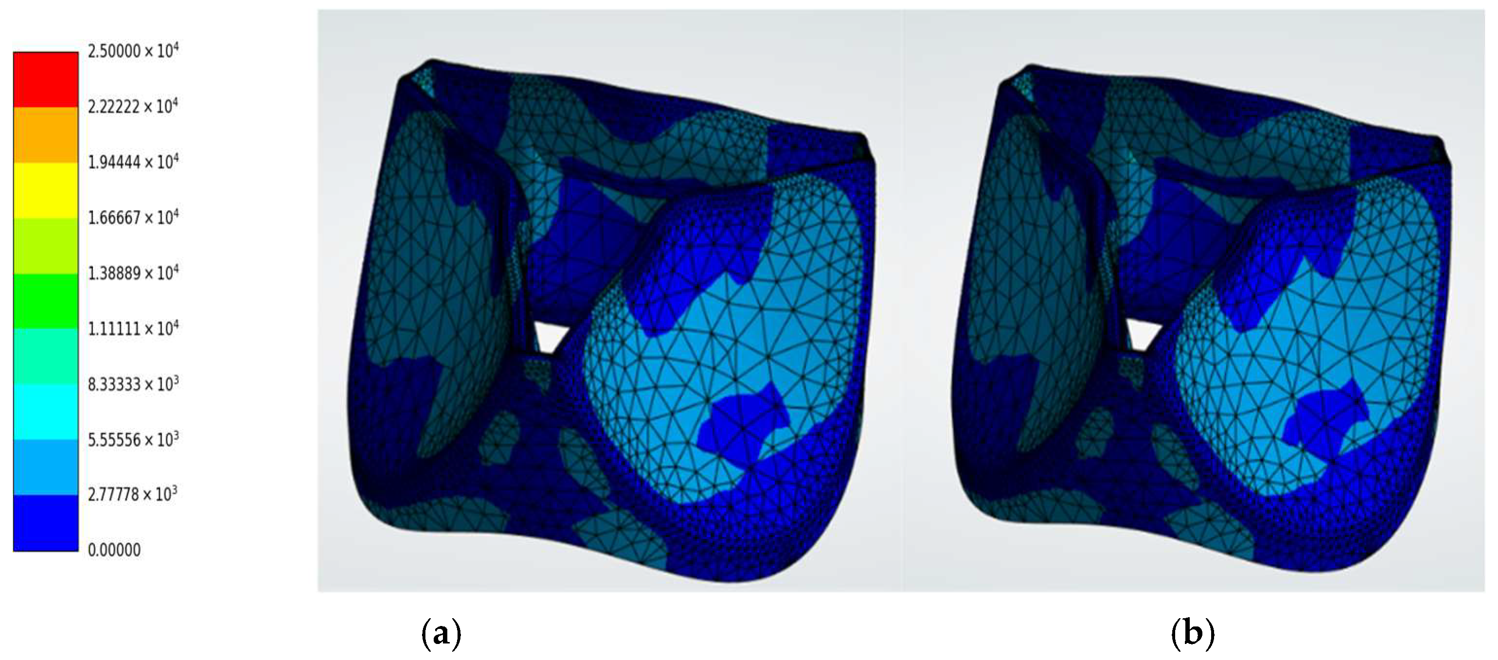
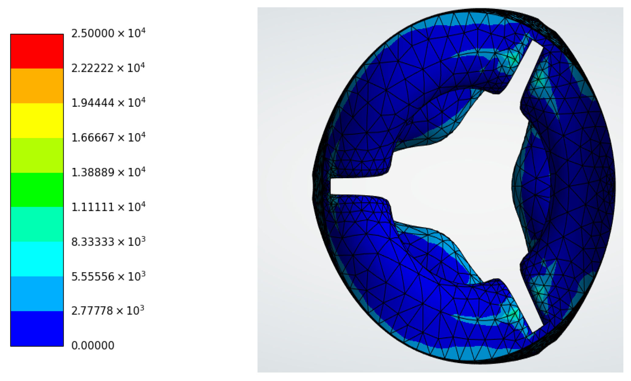
The shear stress distributions shown in Figure 11 further highlight regions of stress transfer across the valve leaflets. The maximum shear stress reached 1.7880 × 10⁴ Pa for pyrolytic carbon (Figure 11a), 2.0937 × 10⁴ Pa for polyurethane (Figure 11b), 1.5128 × 10⁴ Pa for porcine tissue (Figure 11c), and 1.5237 × 10⁴ Pa for bovine tissue (Figure 11d). These stresses were concentrated along the leaflet curvature and commissural attachments.
  • Viscoelastic Materials
The stress distributions for the viscoelastic materials are shown in Figure 11, Figure 12 and Figure 13. Compared with the linear elastic models, viscoelastic formulations reduced the predicted von Mises stress values due to stress relaxation effects.
Von-Mises stress
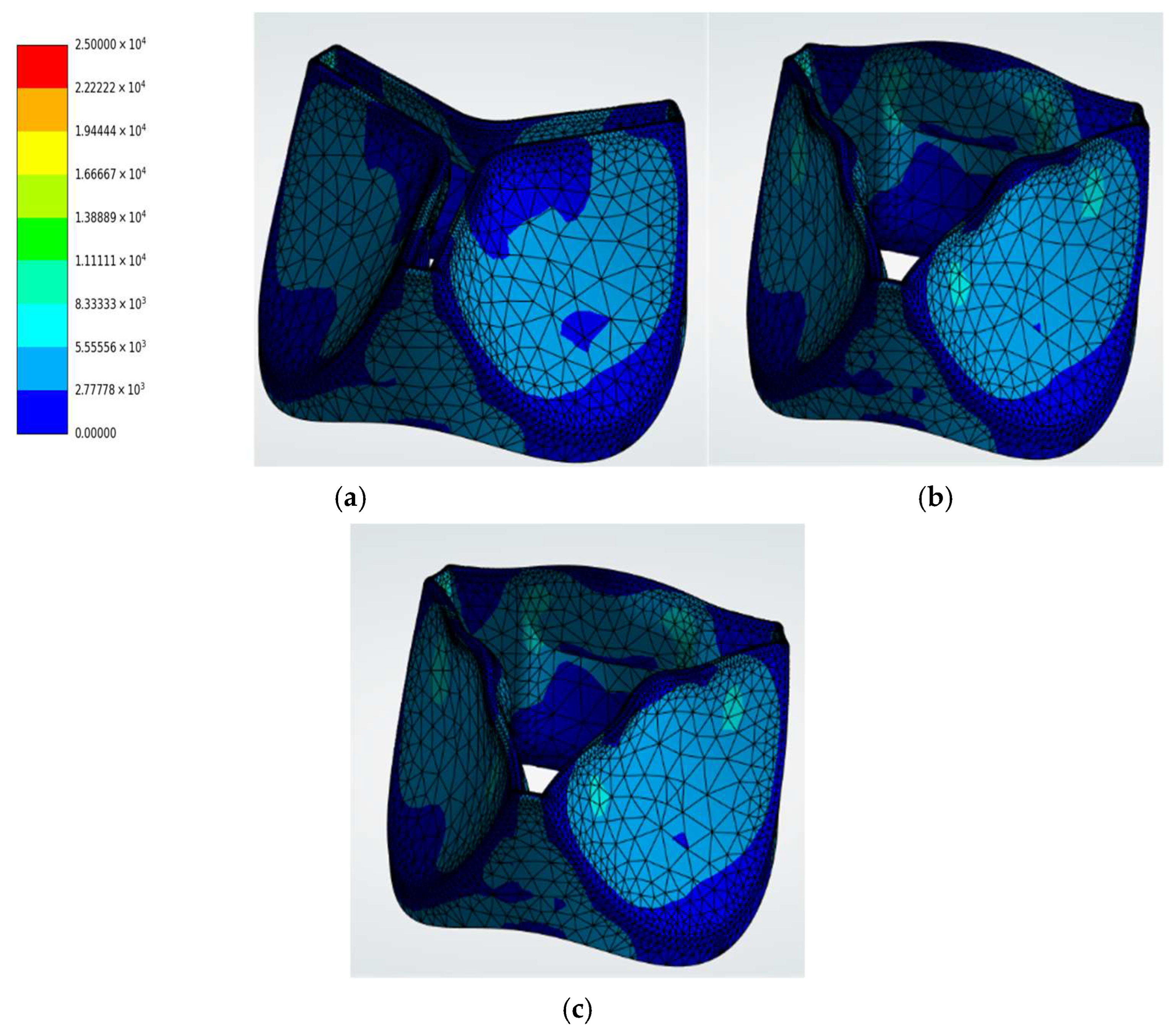
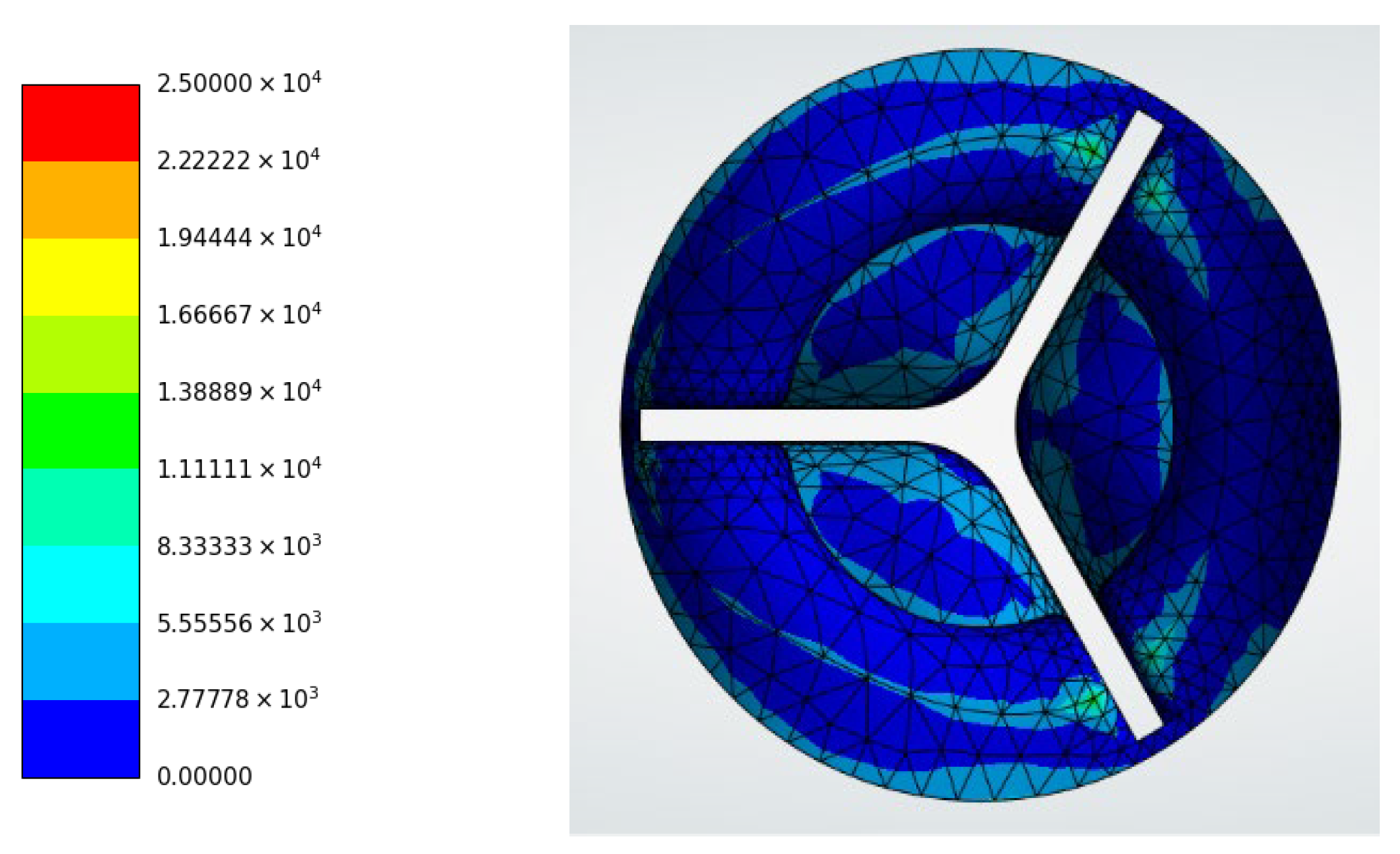
Polyurethane (Figure 12a) exhibited a maximum von Mises stress of 2.1557 × 10⁴ Pa, while porcine (Figure 12b) and bovine (Figure 12c) exhibited stresses of 2.2118 × 10⁴ Pa and 2.2864 × 10⁴ Pa, respectively, as shown in Figure 12.
Maximum Principal Stress
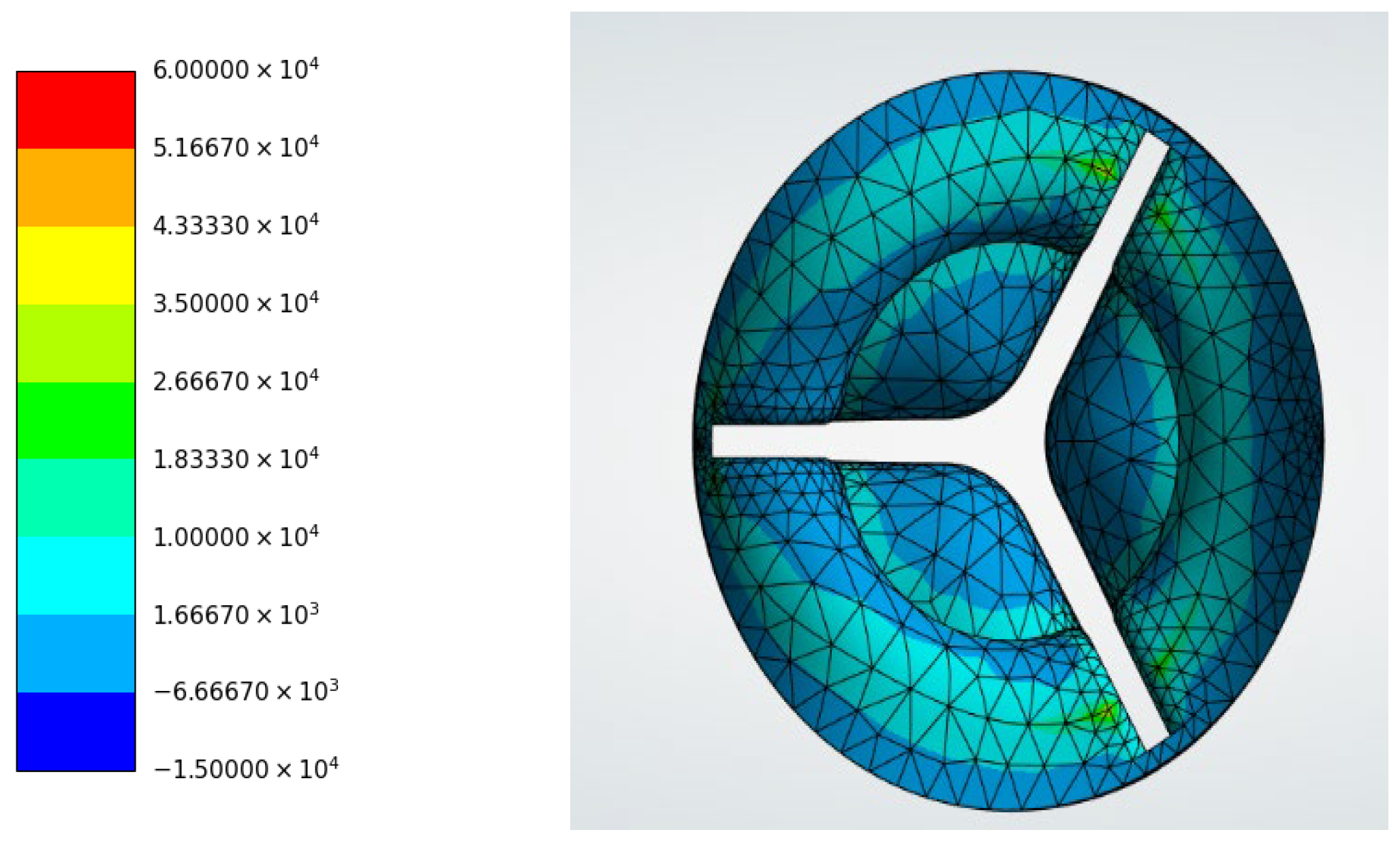
The maximum principal stress contours shown in Figure 13 indicate tensile stress magnitudes of 5.3712 × 10⁴ Pa for polyurethane (Figure 13a), 5.8521 × 10⁴ Pa for porcine (Figure 13b), and 5.6551 × 10⁴ Pa for bovine (Figure 13c).
Maximum Shear Stress
The shear stress distributions shown in Figure 14 revealed maximum values of 1.0836 × 10⁴ Pa for polyurethane (Figure 14a), 1.1367 × 10⁴ Pa for porcine (Figure 14b, and 1.1705 × 10⁴ Pa for bovine (Figure 14c), respectively.
Hyperelastic Materials
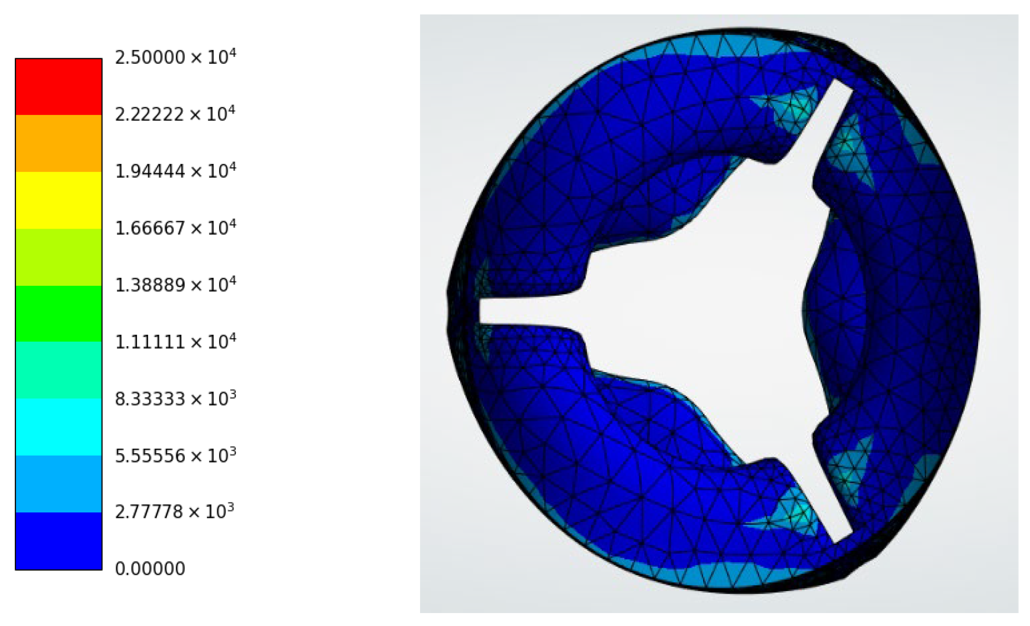
The hyperelastic stress distributions are presented in Figure 15 and Figure 16.
Von-Mises stress
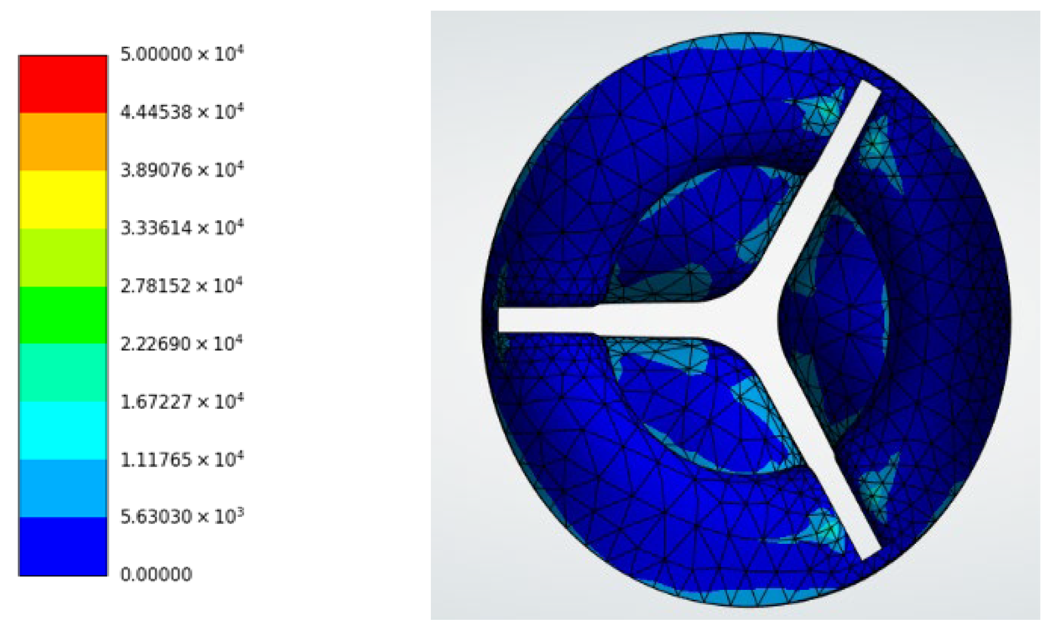
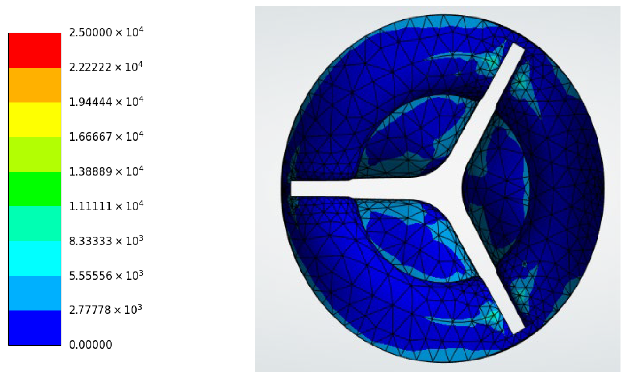
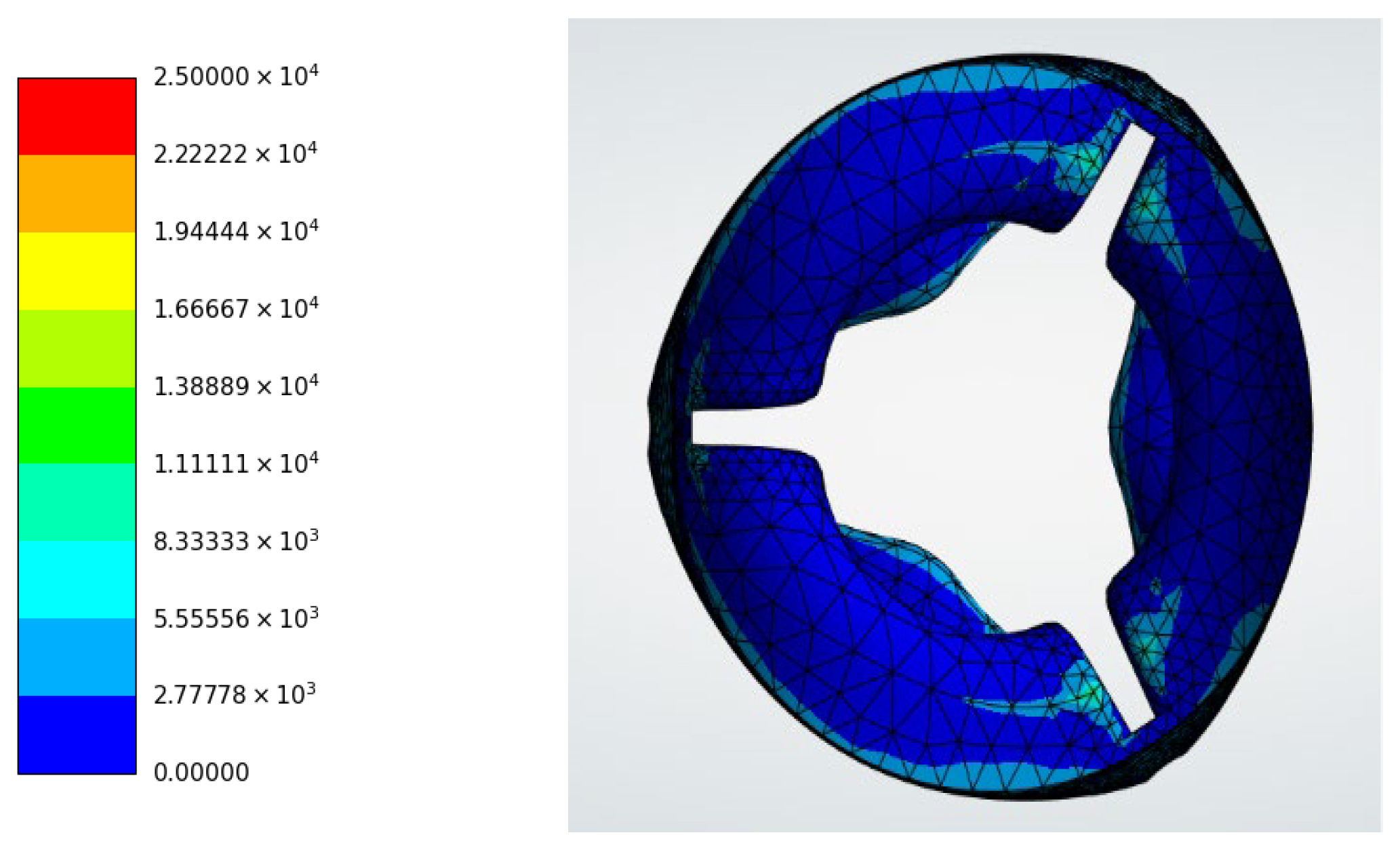
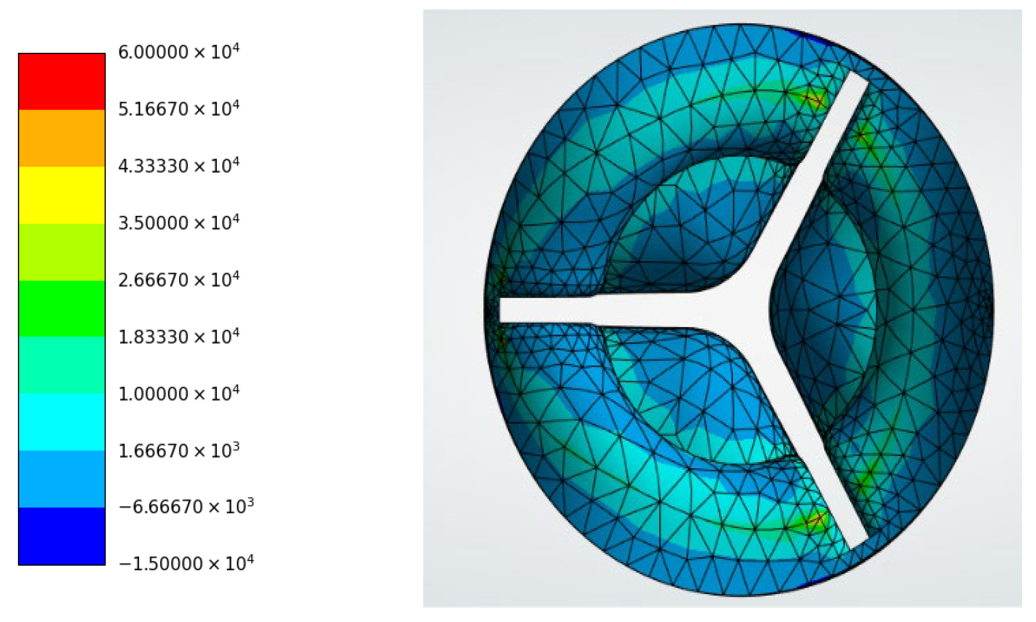
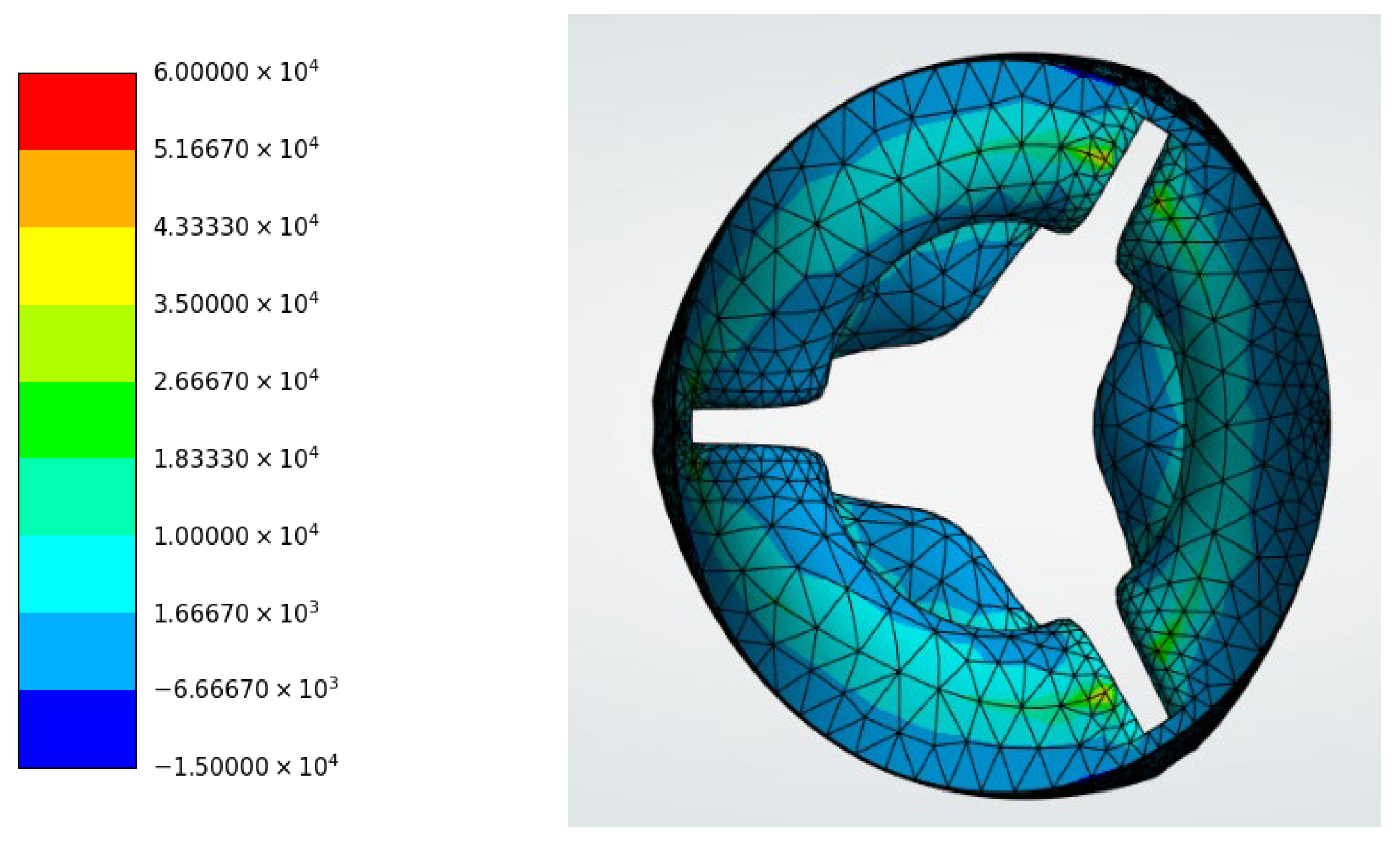
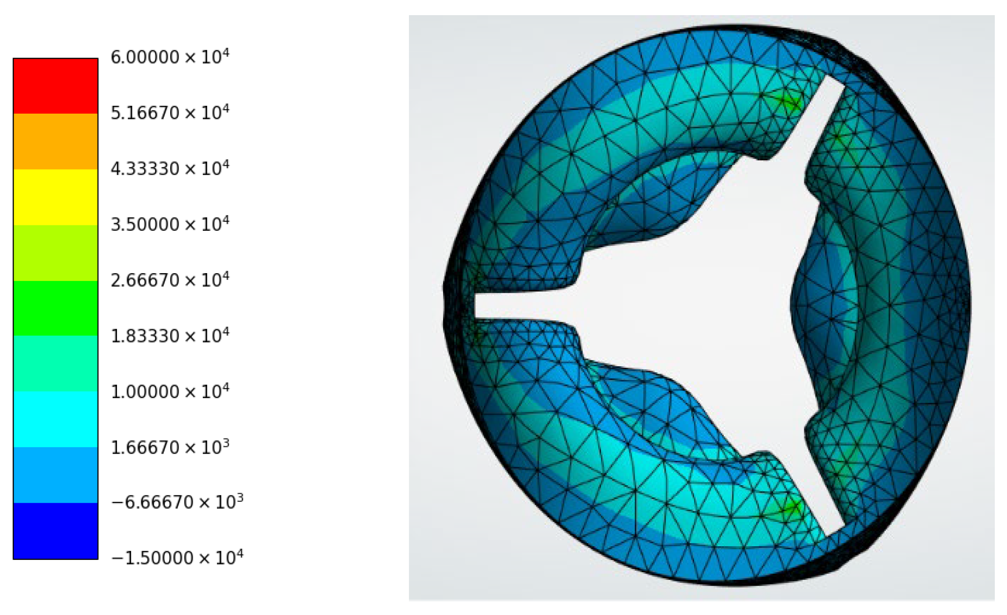
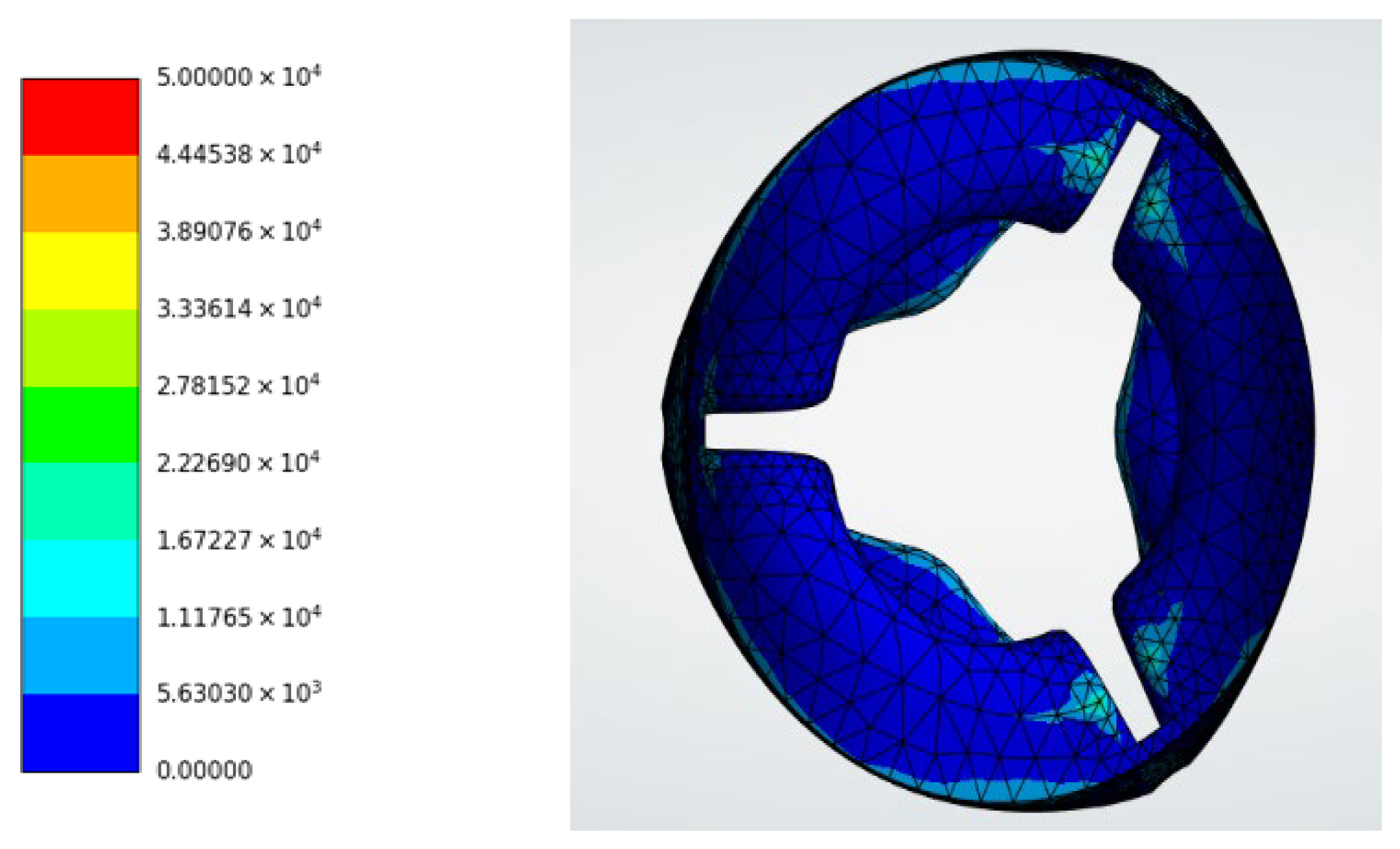
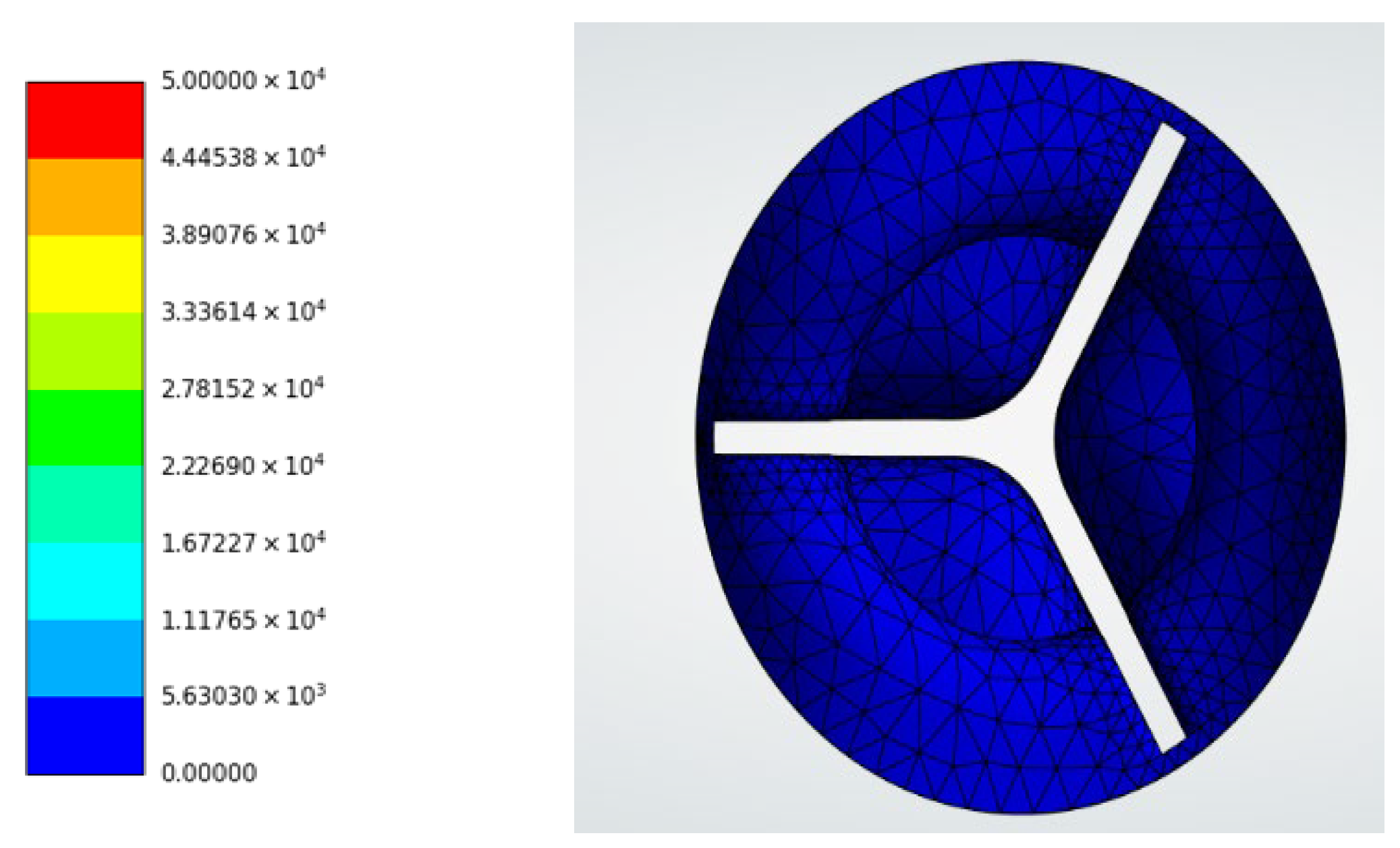
The porcine hyperelastic model (Figure 15a) exhibited a von Mises stress of 1.3951 × 10⁴ Pa, while the bovine hyperelastic model (Figure 15b) exhibited 1.8603 × 10⁴ Pa. These values are lower than those predicted by the linear elastic models, indicating that nonlinear material behavior allows improved stress redistribution under deformation.
Maximum Principal Stress
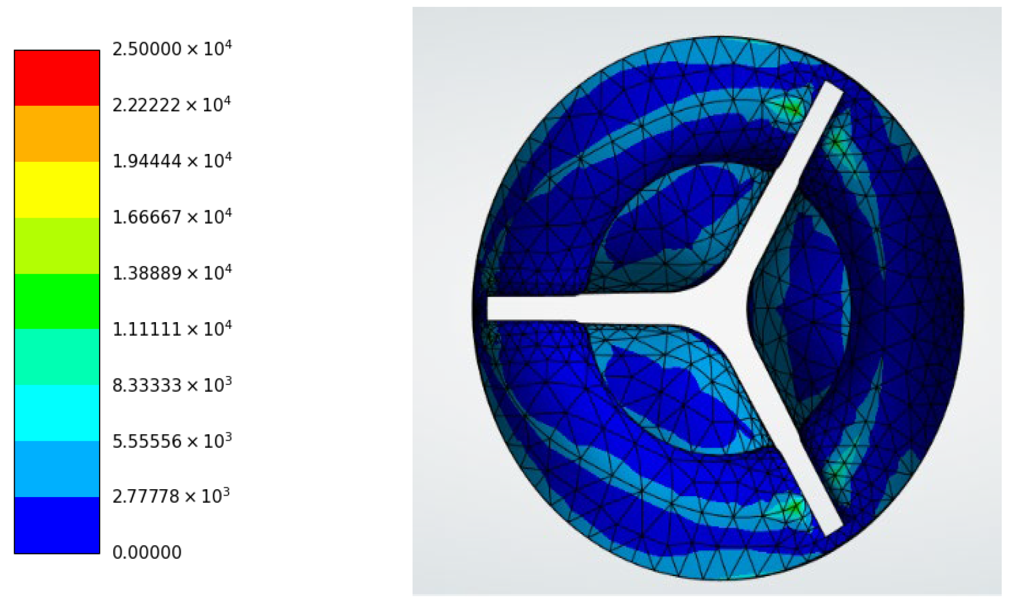
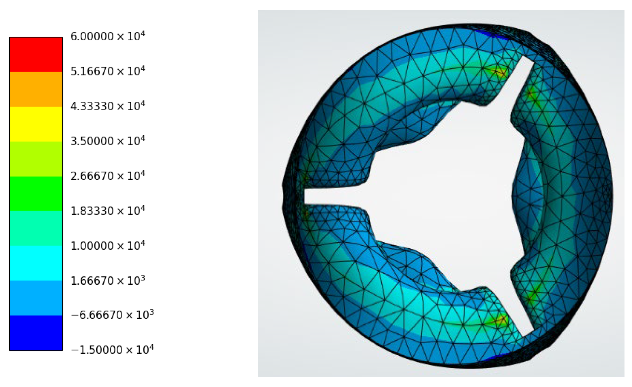
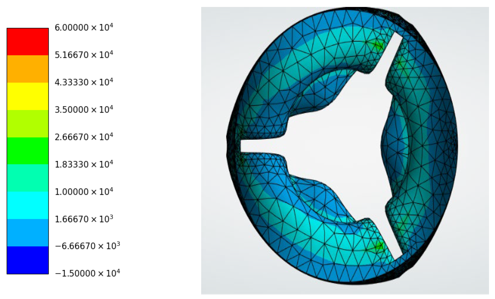
The principal stress distributions shown in Figure 16 reached 2.8815 × 10⁴ Pa for porcine (Figure 16a) and 2.9423 × 10⁴ Pa for bovine (Figure 16b).
Maximum Shear Stress
The shear stress contours in Figure 17 showed maximum values of 9.2030 × 10³ Pa for porcine (Figure 17a) and 9.3911 × 10³ Pa for bovine (Figure 17b), respectively.

3.1.3. Strain and Energy Distribution

Linear Elastic Materials
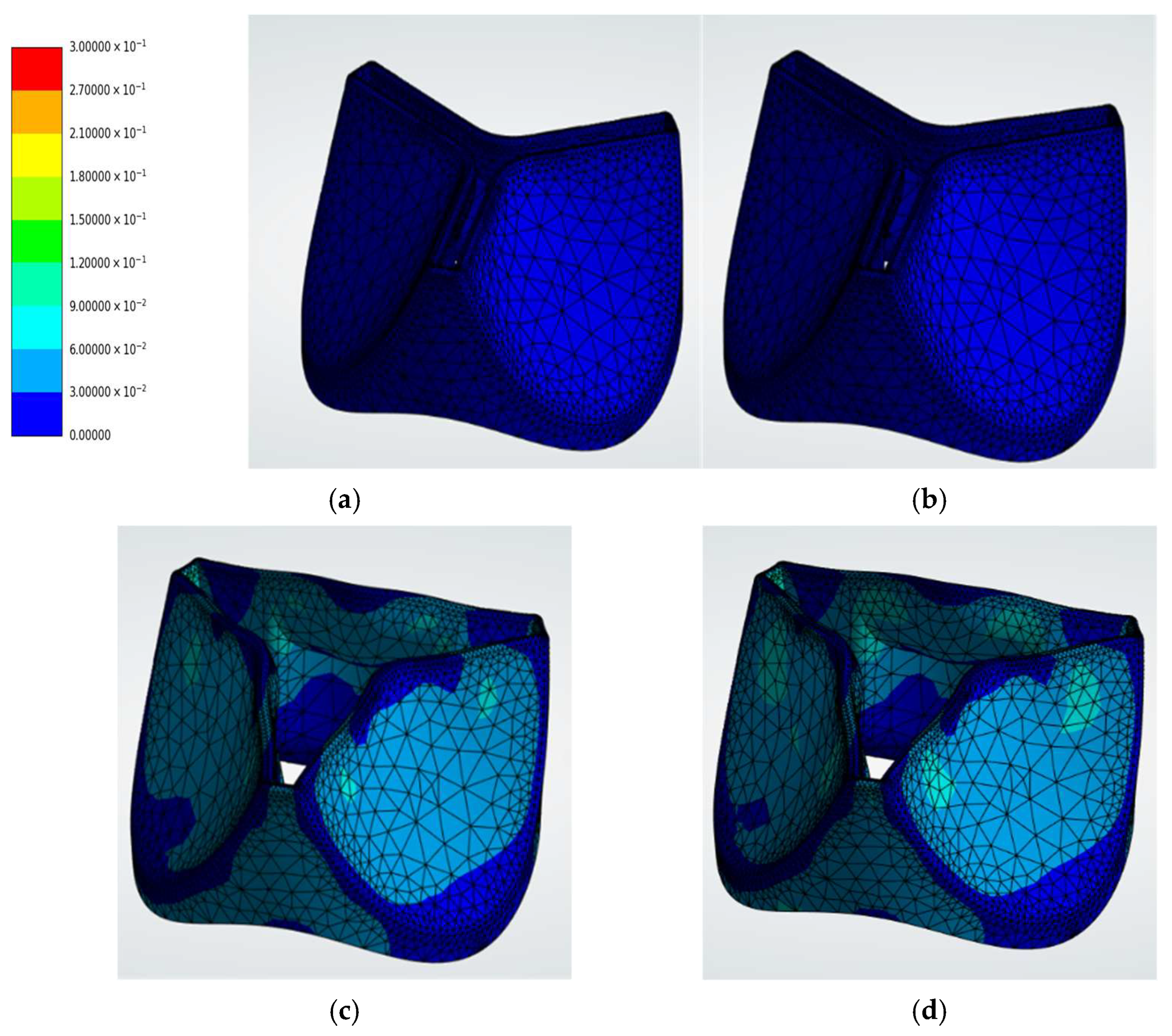
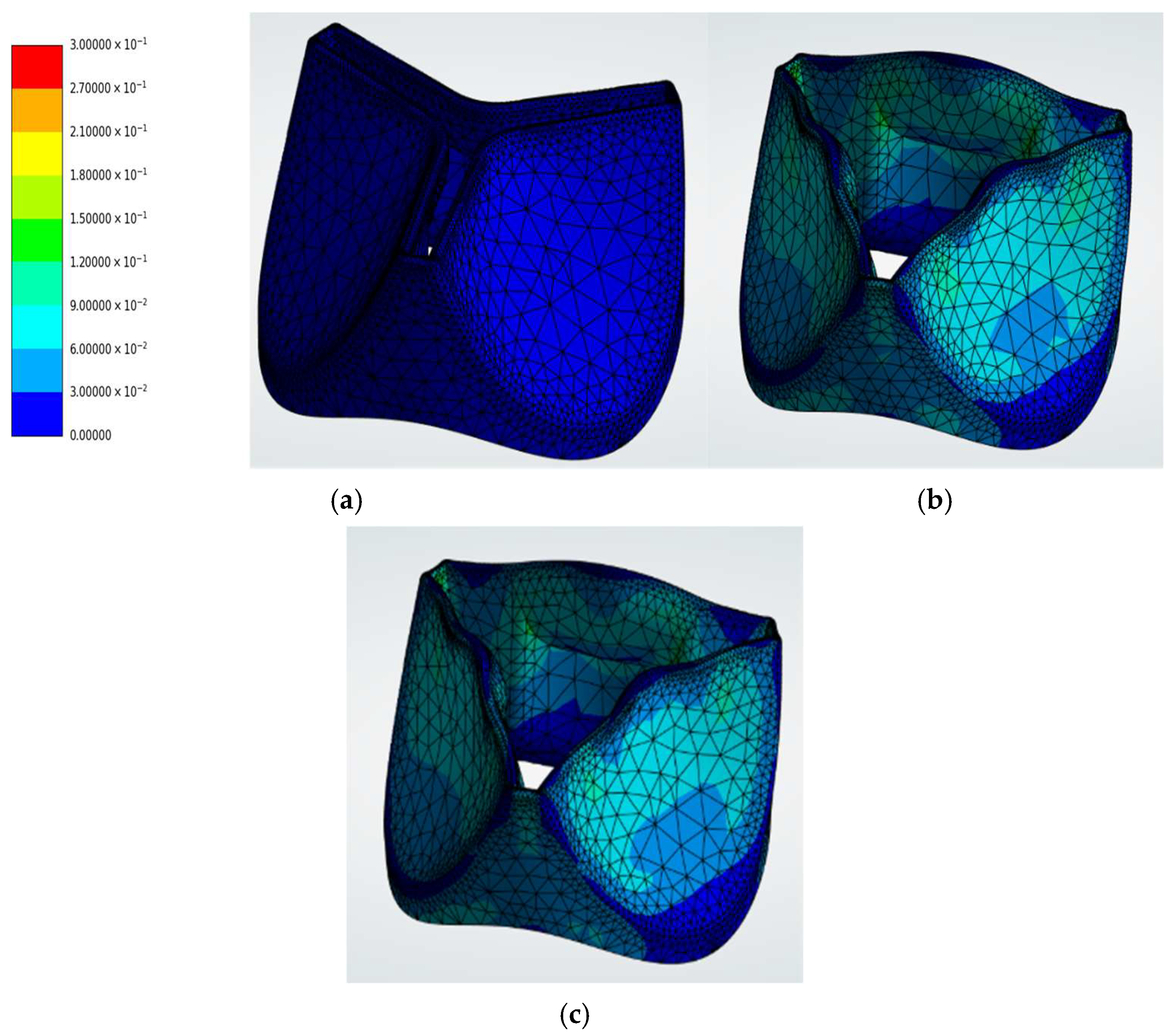
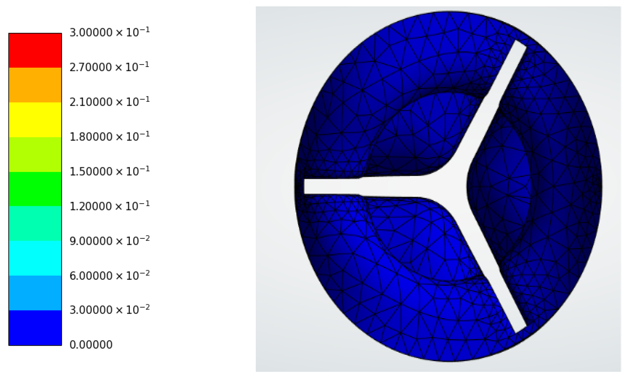
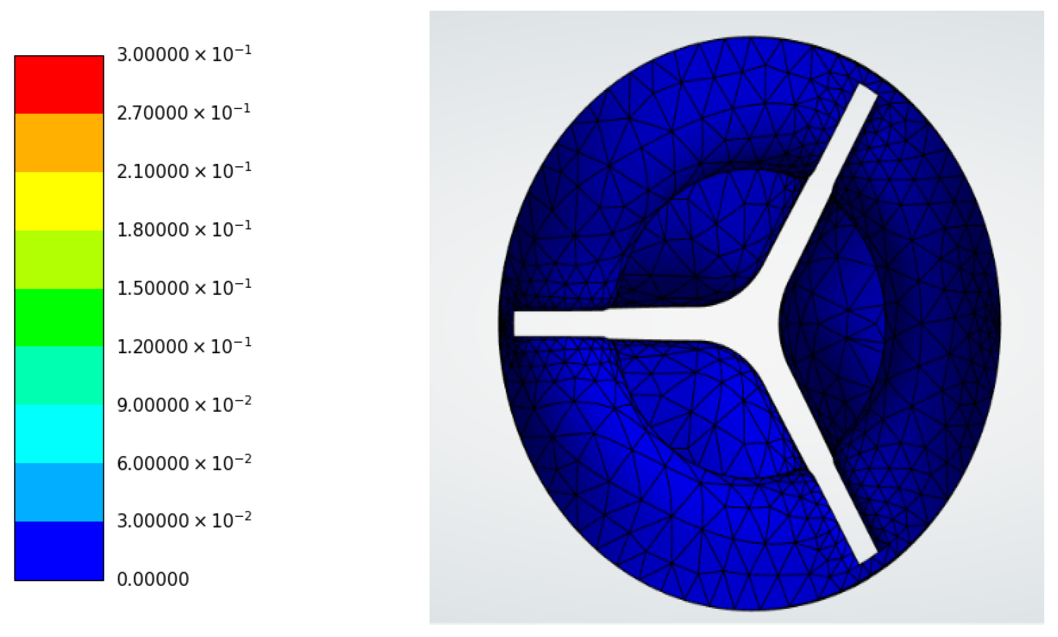
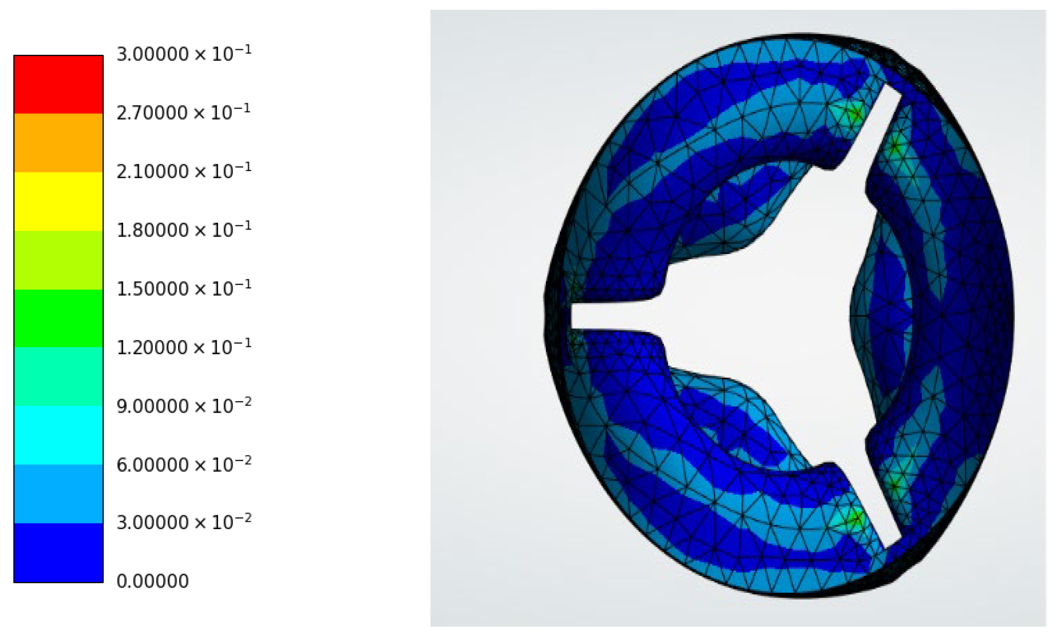
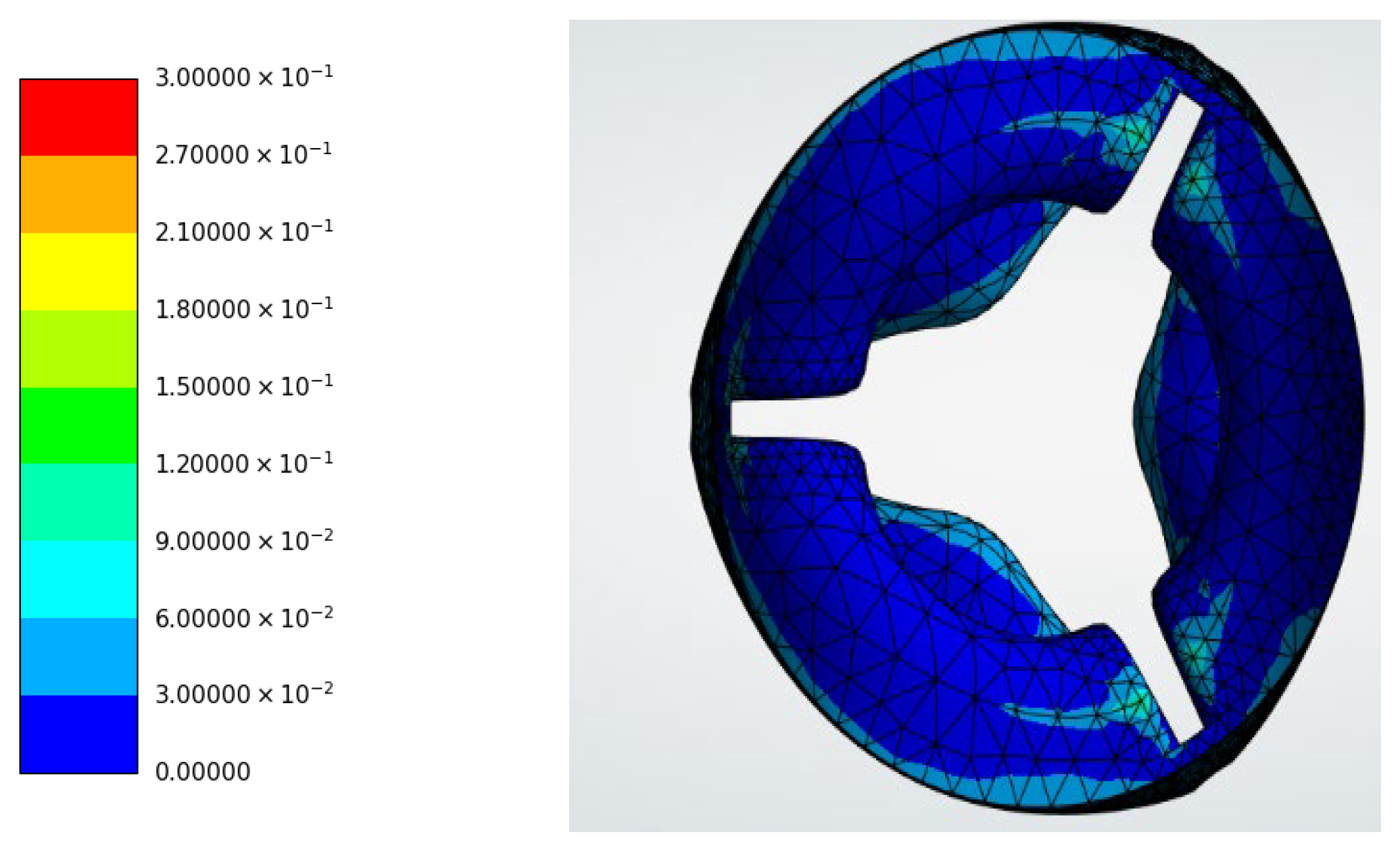
The equivalent strain distributions for the linear elastic materials are shown in Figure 18. Pyrolytic carbon (Figure 18a) exhibited extremely small strain (1.2153 × 10⁻⁶), confirming its rigid mechanical behavior. Polyurethane (Figure 18b) showed moderate strain (2.6812 × 10⁻²), while biological tissues exhibited significantly higher strain levels.
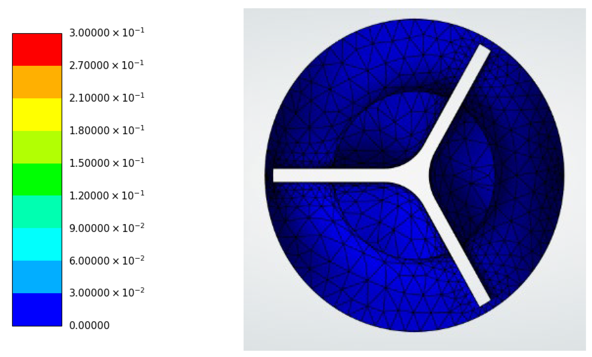
The porcine linear elastic model (Figure 18c) exhibited a maximum equivalent strain of 1.8710 × 10⁻¹, while the bovine linear elastic model (Figure 18d) exhibited 2.0399 × 10⁻¹, indicating greater flexibility of biological tissues compared with synthetic materials.
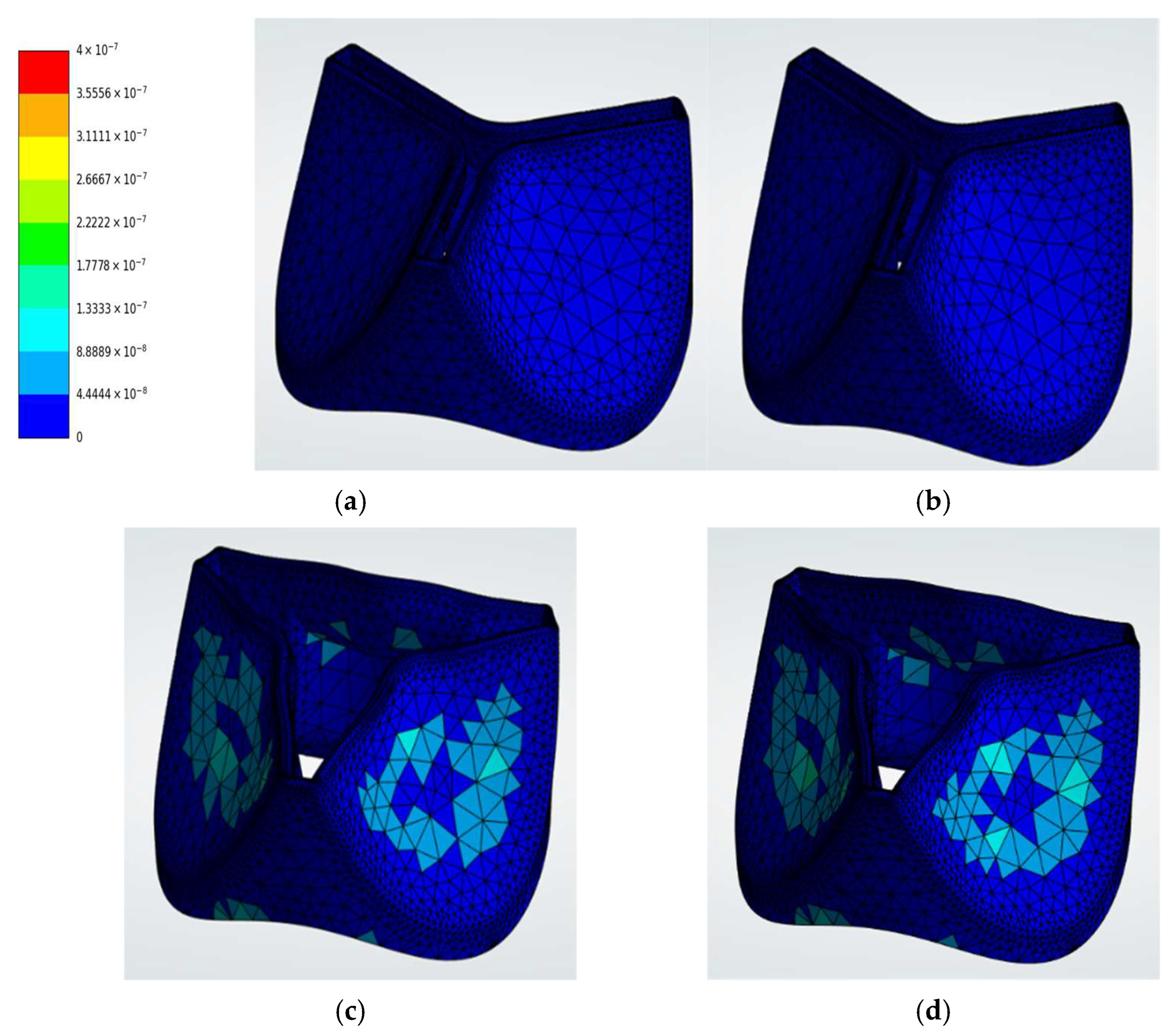
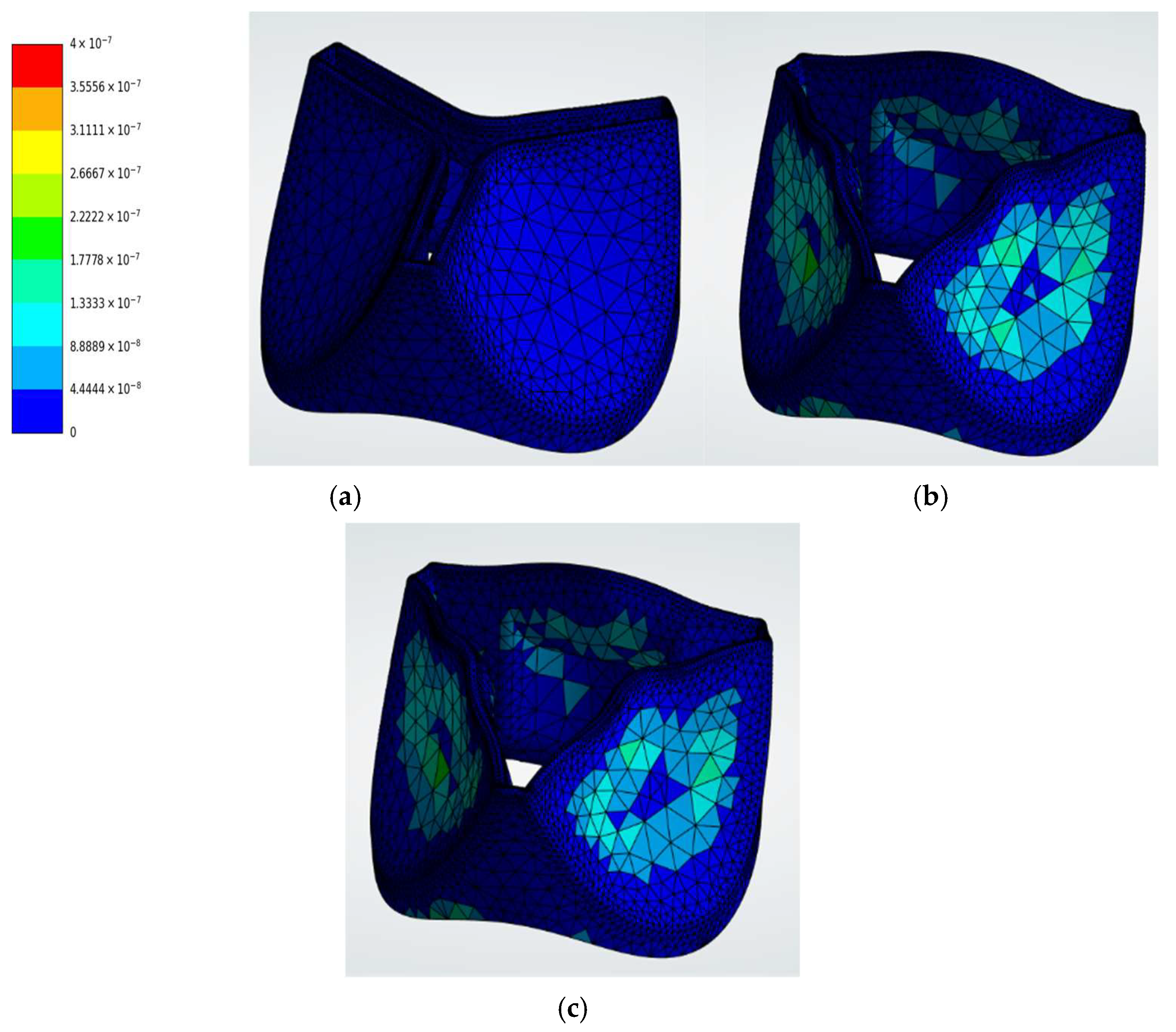
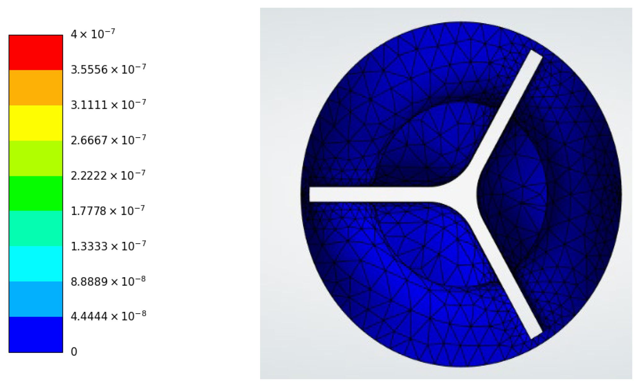
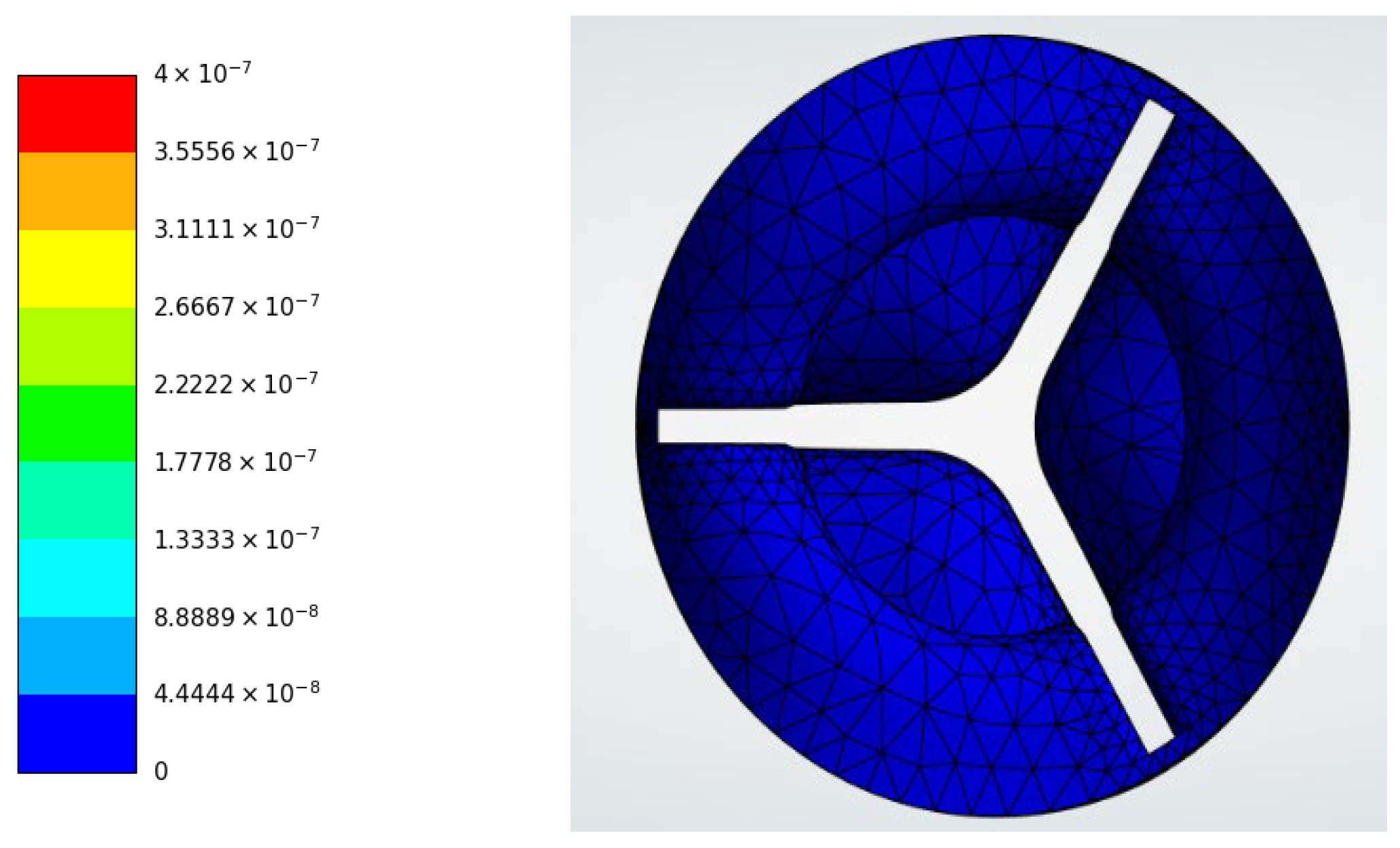
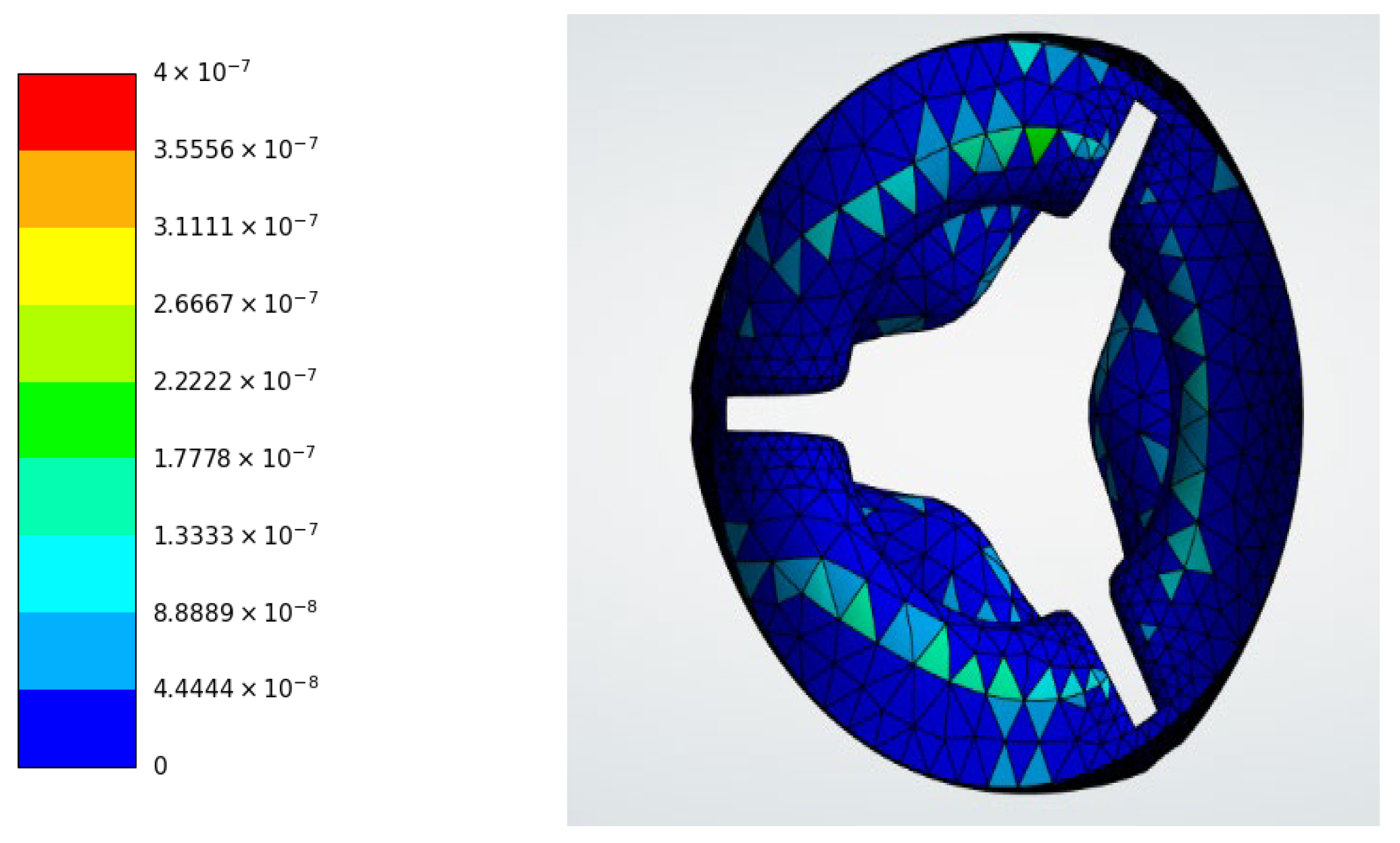
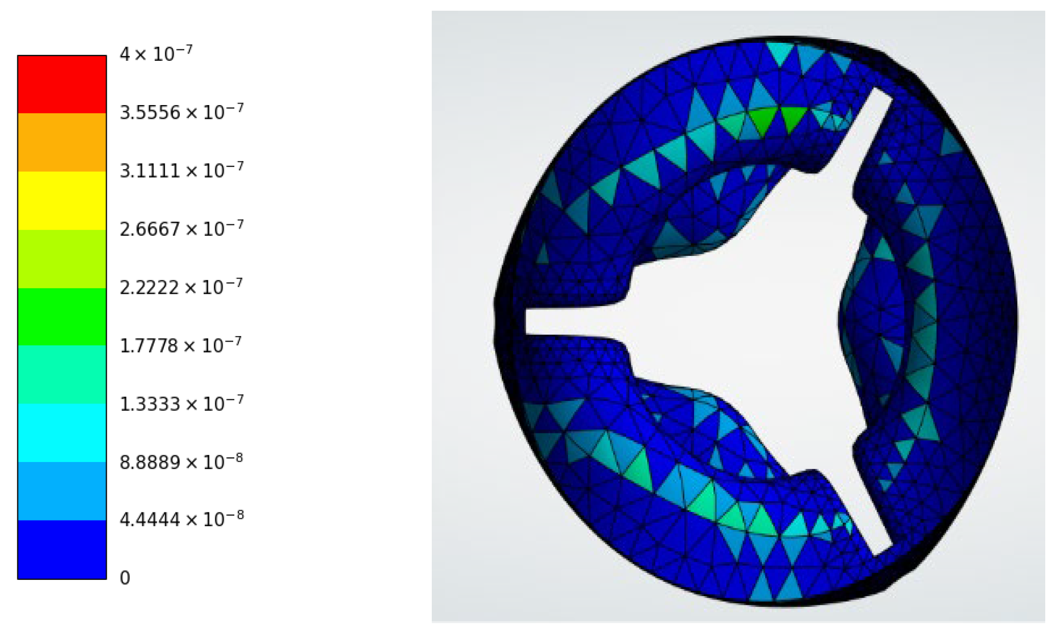
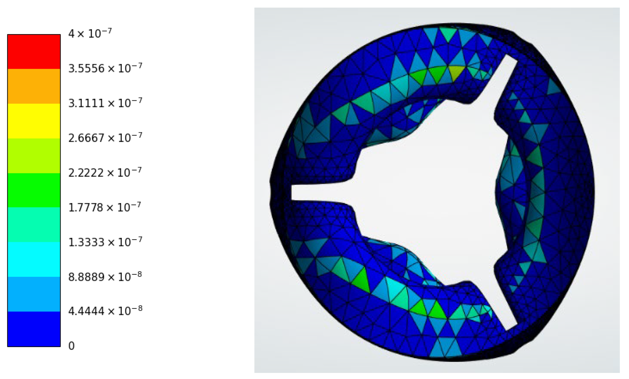
The strain energy distributions shown in Figure 19 indicate the amount of elastic energy stored within the valve leaflets during deformation. Pyrolytic carbon (Figure 19a) exhibited negligible strain energy (2.2149 × 10⁻¹² J), whereas polyurethane (Figure 19b) stored 4.0510 × 10⁻⁸ J. Biological tissues exhibited significantly higher strain energy values, reaching 3.6160 × 10⁻⁷ J for porcine (Figure 20c) and 3.8541 × 10⁻⁷ J for bovine tissue (Figure 19d).
Viscoelastic Materials
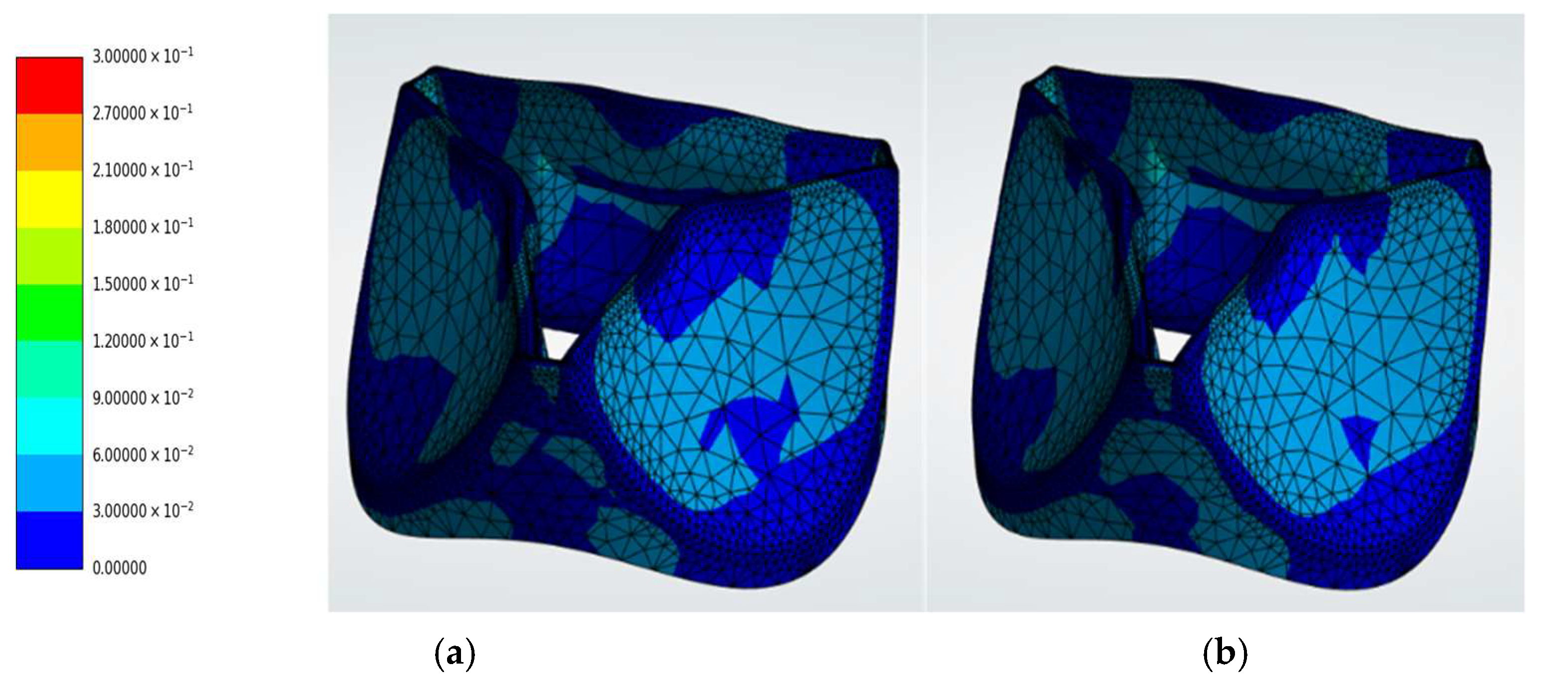
The viscoelastic strain distributions shown in Figure 20 reveal increased strain in biological tissues, with porcine (Figure 20b) reaching 2.5102 × 10⁻¹ and bovine (Figure 20c) reaching 2.4139 × 10⁻¹, while polyurethane (Figure 20a) exhibited 1.9510 × 10⁻².
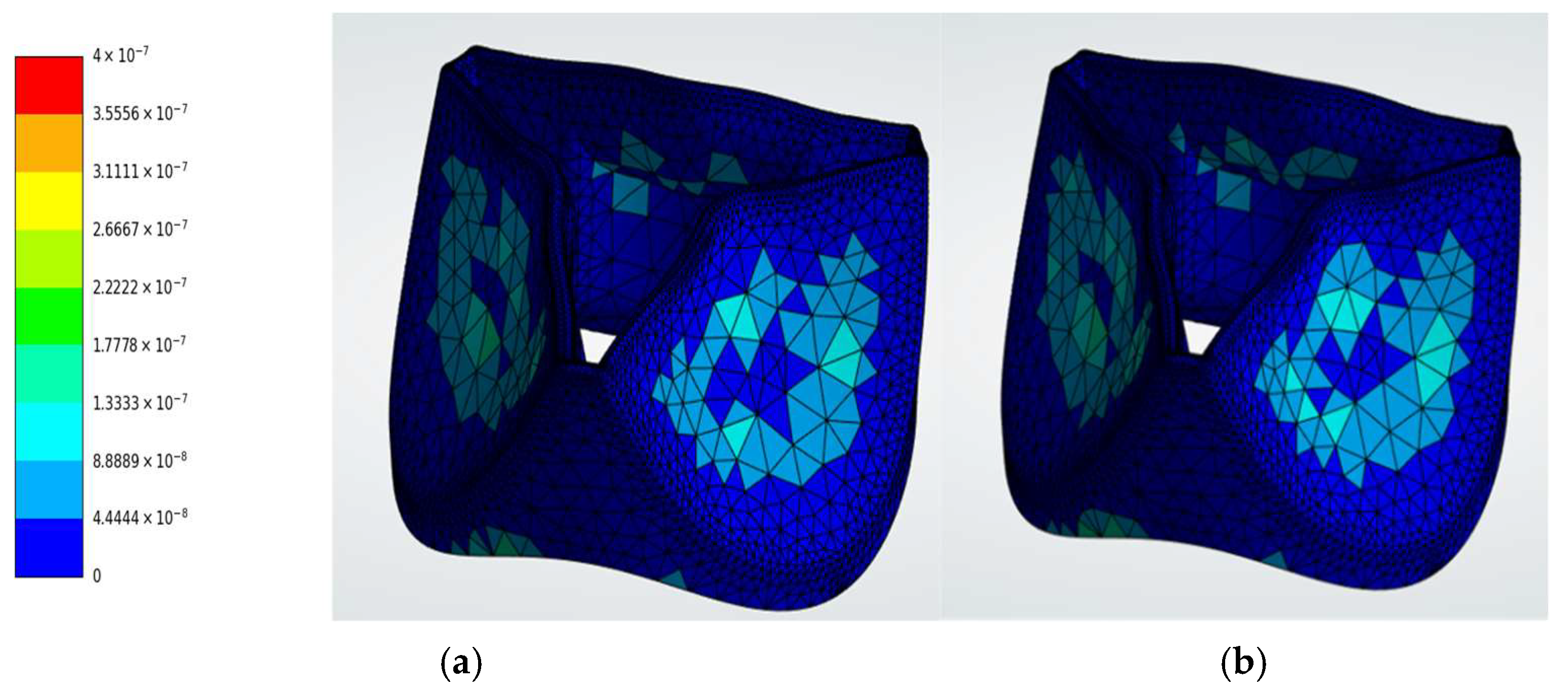
The corresponding strain energy distributions shown in Figure 21 indicate energy storage of 2.1683 × 10⁻⁸ J for polyurethane (Figure 21a), 2.6302 × 10⁻⁷ J for porcine (Figure 21b), and 2.6217 × 10⁻⁷ J for bovine (Figure 21c).
Hyperelastic Materials
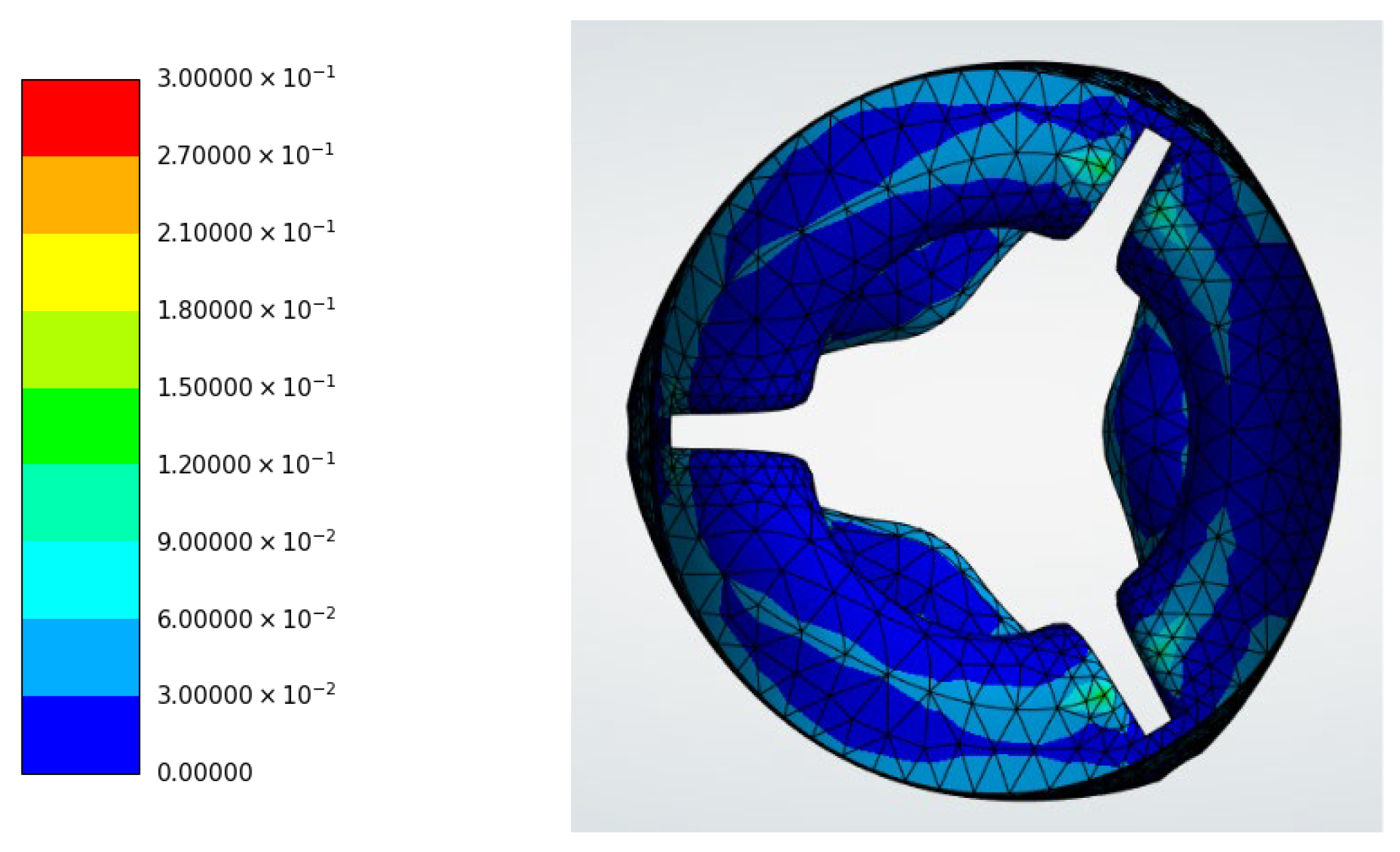
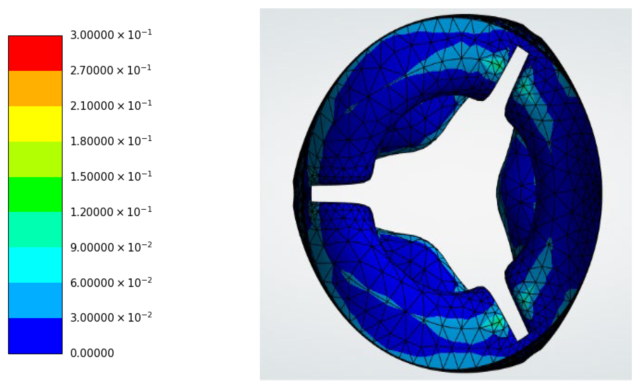
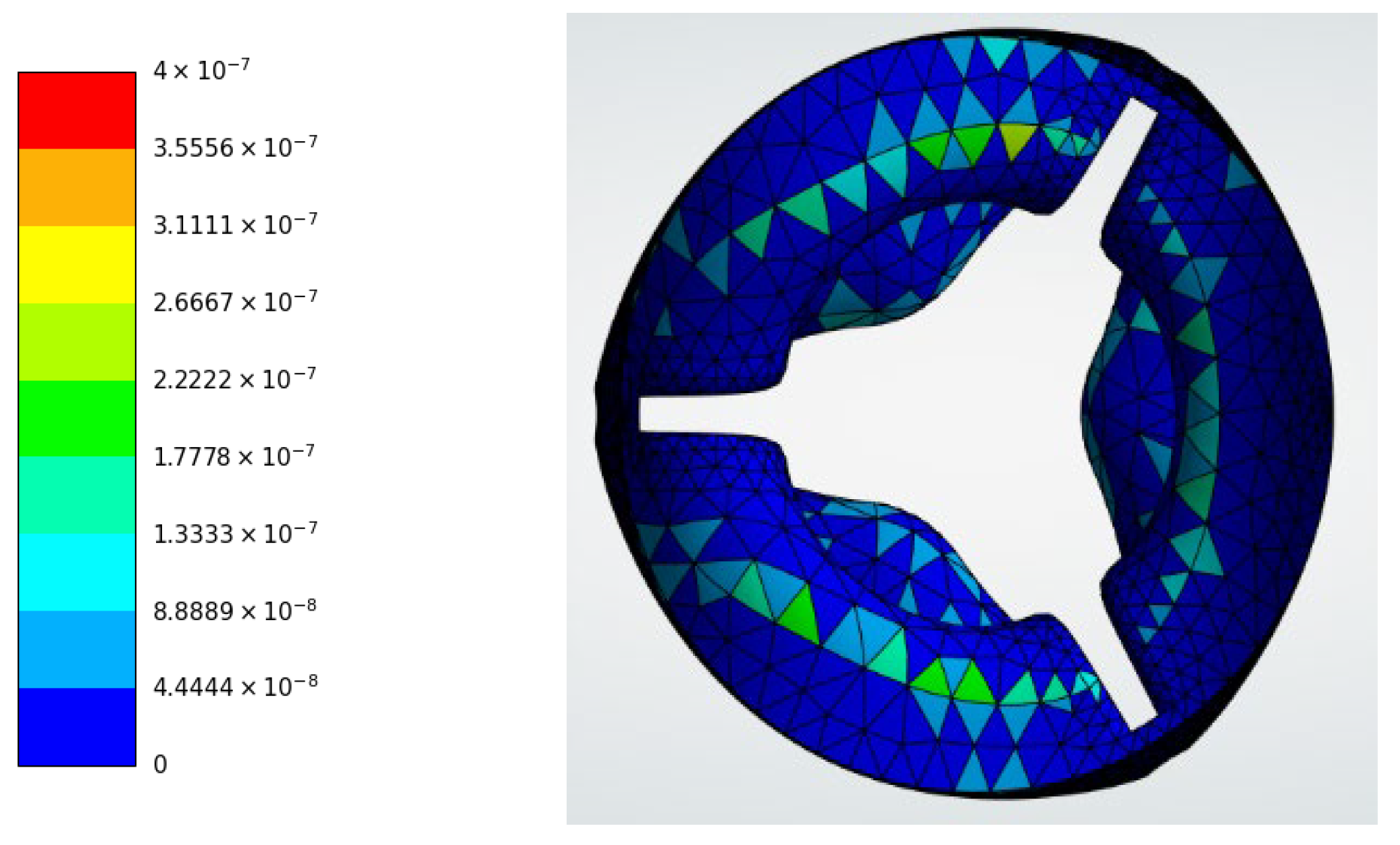
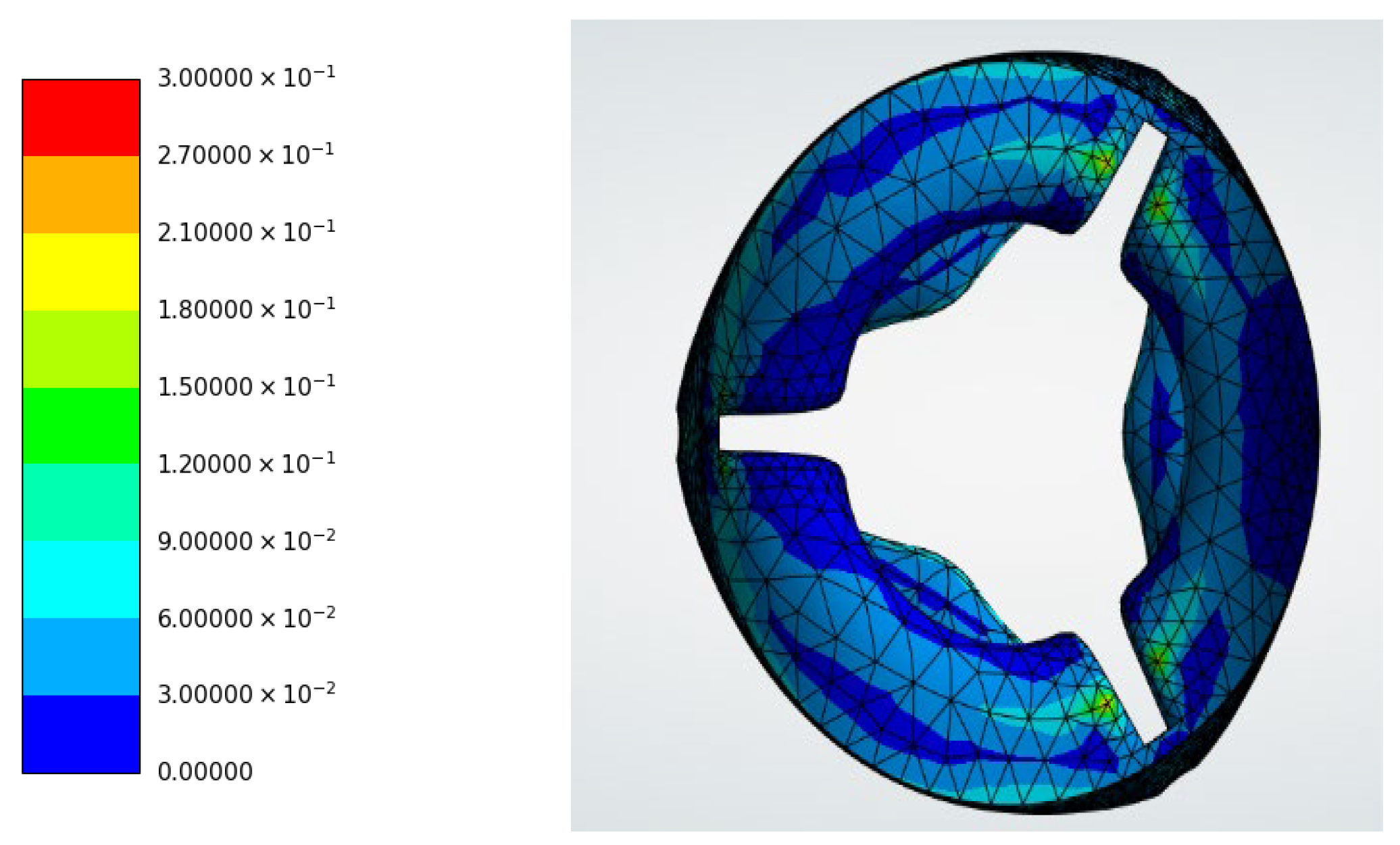
For the hyperelastic material models, the strain distributions shown in Figure 22 indicate equivalent strain values of 1.3287 × 10⁻¹ for porcine (Figure 22a) and 1.4204 × 10⁻¹ for bovine (Figure 22b). The strain energy contours shown in Figure 23 demonstrate stored energy values of 2.5339 × 10⁻⁷ J for porcine (Figure 23a) and 2.6847 × 10⁻⁷ J for bovine (Figure 23b), respectively.
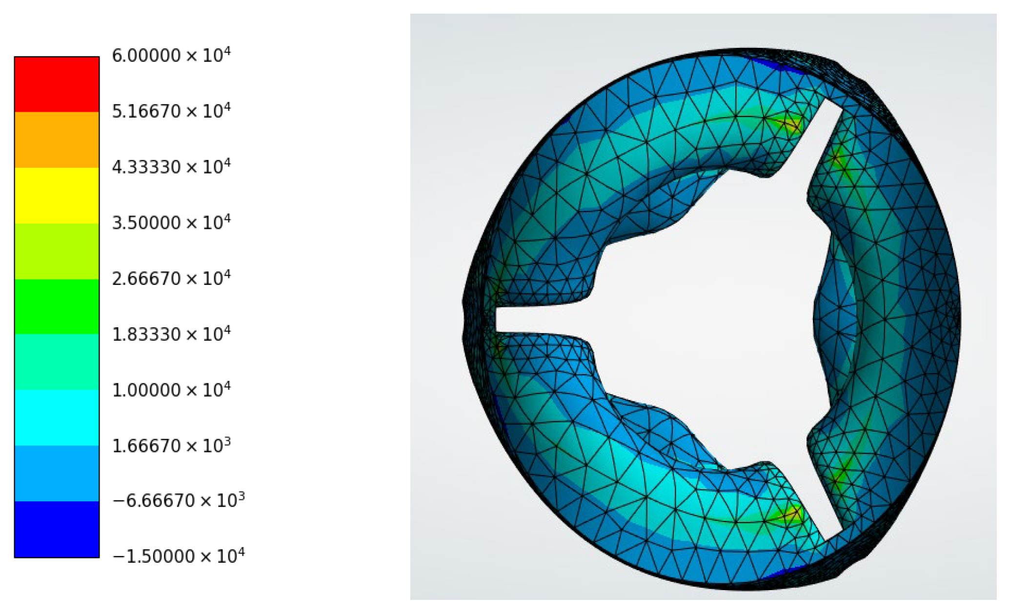
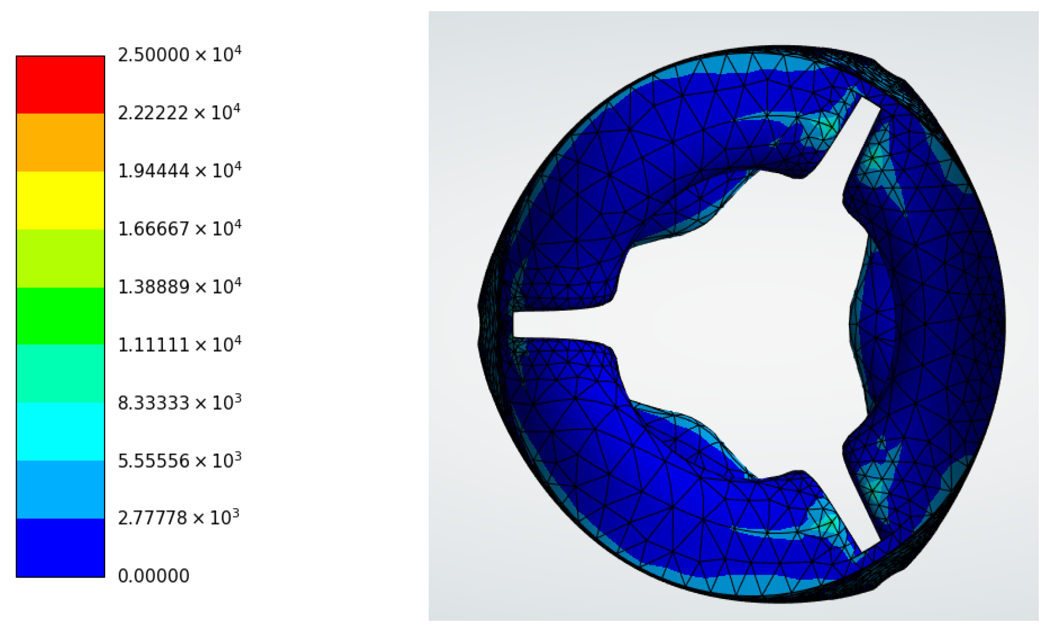
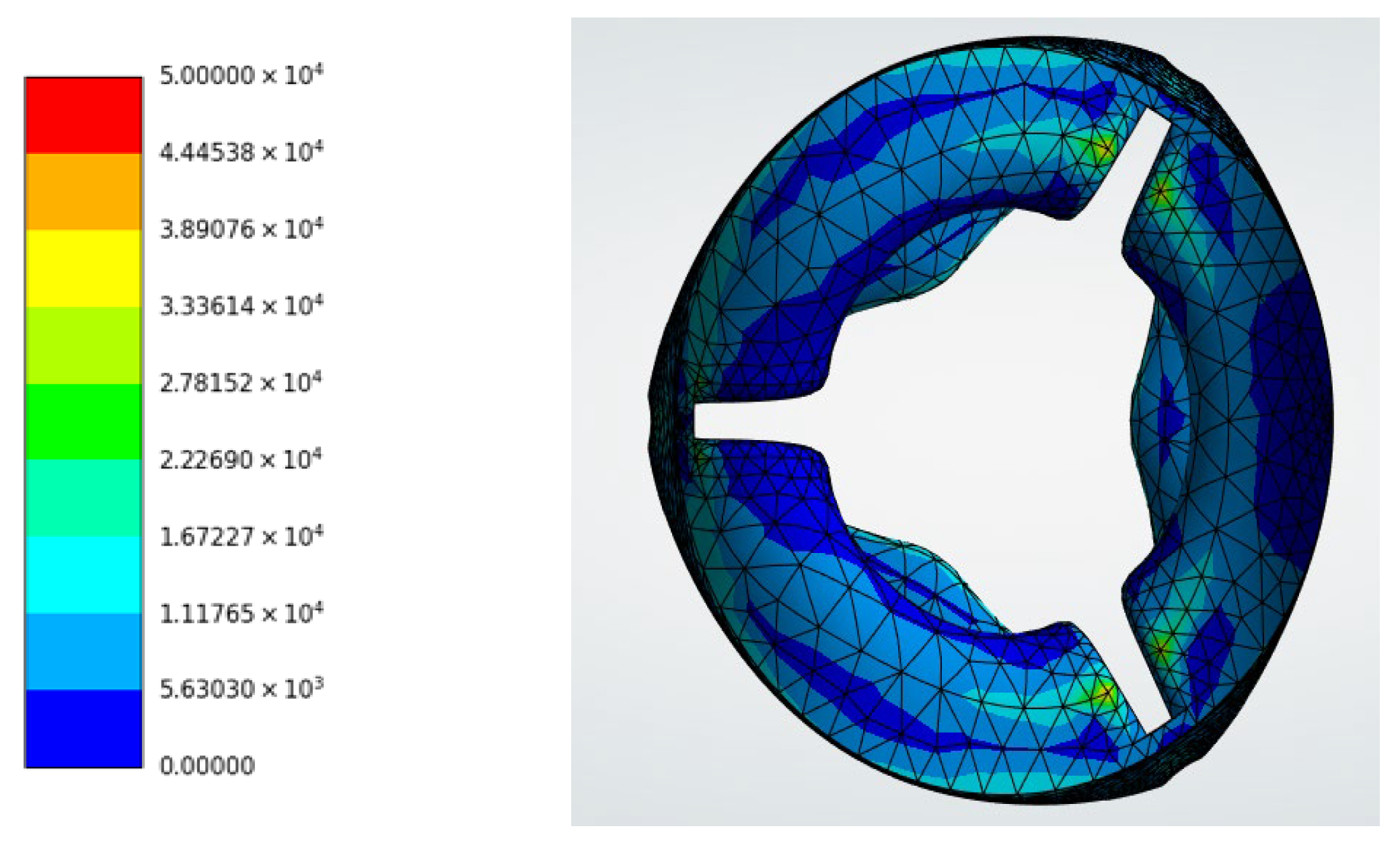
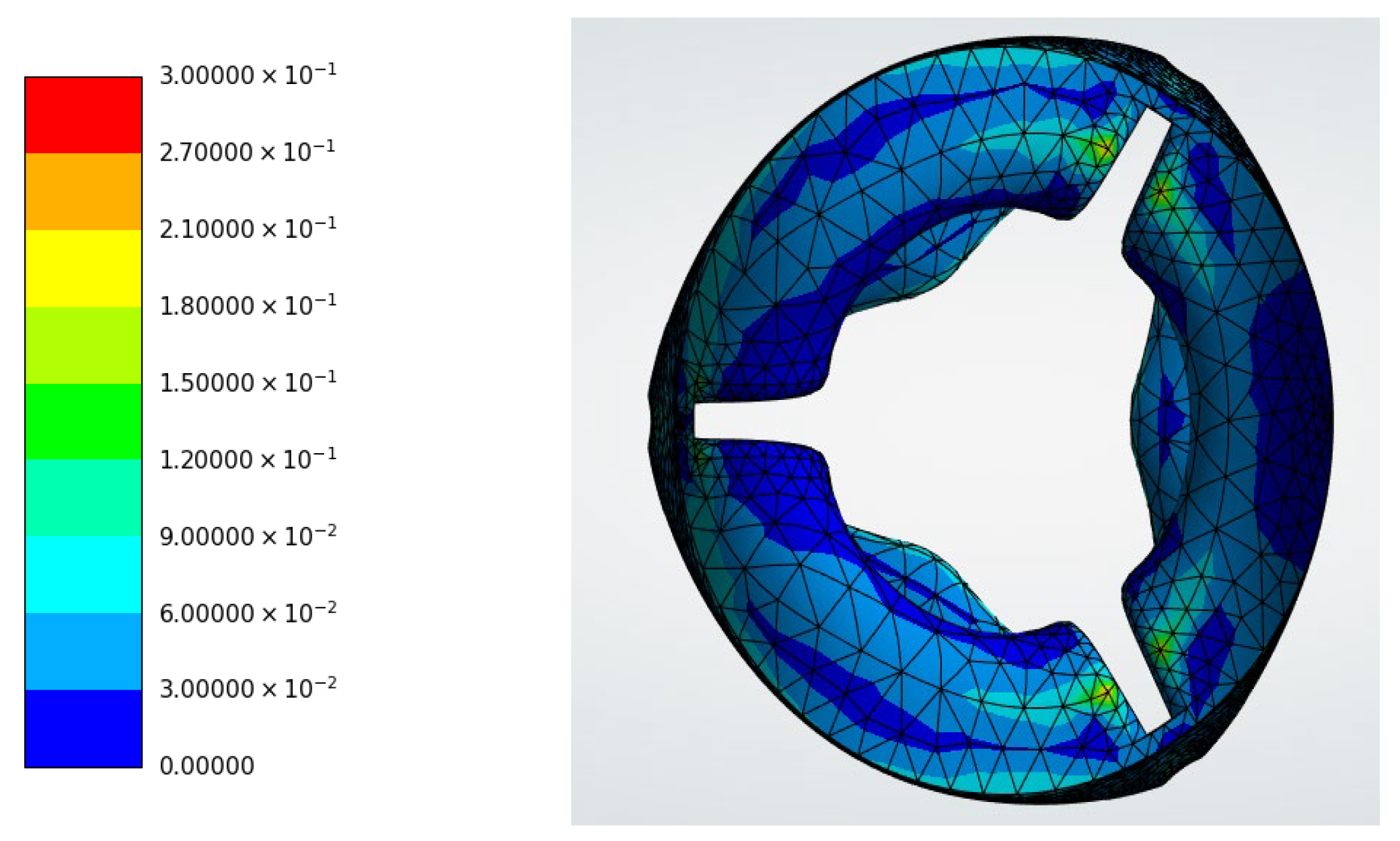
The comparative results summarized in Table 1 demonstrate a clear dependence of valve mechanics on material stiffness and constitutive formulation. Among all materials, pyrolytic carbon exhibited the smallest deformation (1.7166 × 10⁻⁸ m) and strain (1.2153 × 10⁻⁶), confirming its functionally rigid behavior. In contrast, the biological tissues exhibited the highest strain levels and strain-energy storage, while the largest deformation in the present rerun was observed for the bovine hyperelastic model (9.6837 × 10⁻⁵ m). Polyurethane demonstrated intermediate mechanical behavior, with deformation values on the order of 10−5 m, indicating greater compliance than pyrolytic carbon but lower strain and energy accumulation than the tissue models. Hyperelastic constitutive models for biological tissues resulted in lower peak von Mises stresses (1.3951 × 10⁴–1.8603 × 10⁴ Pa) compared with linear elastic predictions (2.6842 × 10⁴–2.7017 × 10⁴ Pa), demonstrating the ability of nonlinear material models to redistribute mechanical stress during large deformation. Overall, these magnitudes and comparative trends are consistent with previous computational studies reporting compliant pericardial tissue behavior and reduced stress under nonlinear constitutive descriptions [38,39,40]. Supplementary contour visualizations from different viewing angles are presented in Appendix A.

3.1.4. Comparative Assessment of Material and Constitutive Models

A comparative assessment was performed to evaluate how the selection of constitutive models influences the predicted mechanical performance of the tricuspid valve.
Sensitivity of Synthetic Materials (PU vs. PyC)
The comparison between linear elastic and viscoelastic models for Polyurethane (PU) revealed a significant impact of time-dependent dissipation. The introduction of the Prony shear relaxation series resulted in an approximately 47% reduction in peak von Mises stress (from 4.0839 × 10⁴ Pa to 2.1557 × 10⁴ Pa) and a modest increase in maximum deformation from 7.6515 × 10⁻⁵ m to 7.8948 × 10⁻⁵ m. This indicates that a purely linear elastic approach overestimates the structural loading on polymeric leaflets by failing to account for the material’s inherent stress-relaxation properties. In contrast, Pyrolytic Carbon (PyC), maintained as a linear elastic baseline, showed negligible deformation (1.7166 × 10⁻⁸ m). The stiffness mismatch between the two synthetic materials remained extreme, with PyC exhibiting a Young’s modulus approximately four orders of magnitude higher than PU, resulting in a functionally rigid response.
Sensitivity of Biological Tissues (Porcine vs. Bovine)
The biological tissues exhibited the highest sensitivity to the modeling framework, particularly when transitioning from linear to hyperelastic and viscoelastic states.
  • Linear vs. Hyperelastic: For porcine tissue, the hyperelastic Mooney–Rivlin model predicted an approximately 48% lower peak stress compared with the linear elastic baseline (1.3951 × 10⁴ Pa vs. 2.6842 × 10⁴ Pa). This supports the interpretation that the nonlinear ‘toe-region’ of the hyperelastic response allows more compliant initial deformation and improved stress redistribution across the leaflet surface, consistent with previous tissue-mechanics studies [38,39,40].
  • Viscoelastic vs. Hyperelastic: For bovine tissue, the viscoelastic and hyperelastic formulations produced comparable deformation magnitudes on the order of 10−4 m, while the hyperelastic case reduced peak von Mises stress from 2.2864 × 10⁴ Pa to 1.8603 × 10⁴ Pa. This suggests that time-dependent relaxation increases compliance, whereas nonlinear constitutive behavior contributes to stress redistribution under transient loading.
Inter-Material Comparison (PyC, PU, Porcine, and Bovine)
Across all materials, a clear hierarchy of mechanical performance emerged:
  • Structural Rigidity: PyC remains the only functionally rigid material, providing maximum durability but zero physiological compliance.
  • Compliance Gradient: Biological tissues (Porcine and Bovine) demonstrated the highest strain and strain-energy storage, with deformation values slightly exceeding those of synthetic PU and the largest value observed for bovine hyperelastic tissue.
  • Energy Dynamics: The strain energy density was highest in the bovine linear model (3.8541 × 10⁻⁷ J) and lowest in PyC (2.2149 × 10⁻¹² J). PU occupied a critical “middle ground”, offering a more balanced energy storage profile (4.0510 × 10⁻⁸ J in the linear elastic case) than mechanical carbon, yet maintaining higher structural stability than the biological xenografts.
These results demonstrate that while biological tissues provide superior physiological coaptation through non-linear and time-dependent mechanics, Polyurethane represents a viable synthetic compromise that mimics tissue-like damping without the extreme compliance that can lead to bioprosthetic tissue prolapse.

3.1.5. Transient Evolution of Maximum Structural Response

To further enrich the structural analysis, the temporal evolution of selected maximum mechanical observables was extracted over the 1 s transient simulation. These plots provide additional insight into the evolution of deformation, stress, strain, and shear stress during the transient loading cycle. These plots complement the contour maps by showing how the peak structural response develops during the transient loading cycle rather than only reporting the final or maximum magnitudes.
Overall, all material models exhibited an initial oscillatory transient response followed by progressive stabilization of the maxima. This behavior reflects the transient loading history and the dynamic adjustment of the leaflet structure during the early part of the simulation. Although the general pattern was similar across all cases, the magnitude of the oscillations, the decay rate, and the stabilized response level depended strongly on the material stiffness and constitutive formulation.
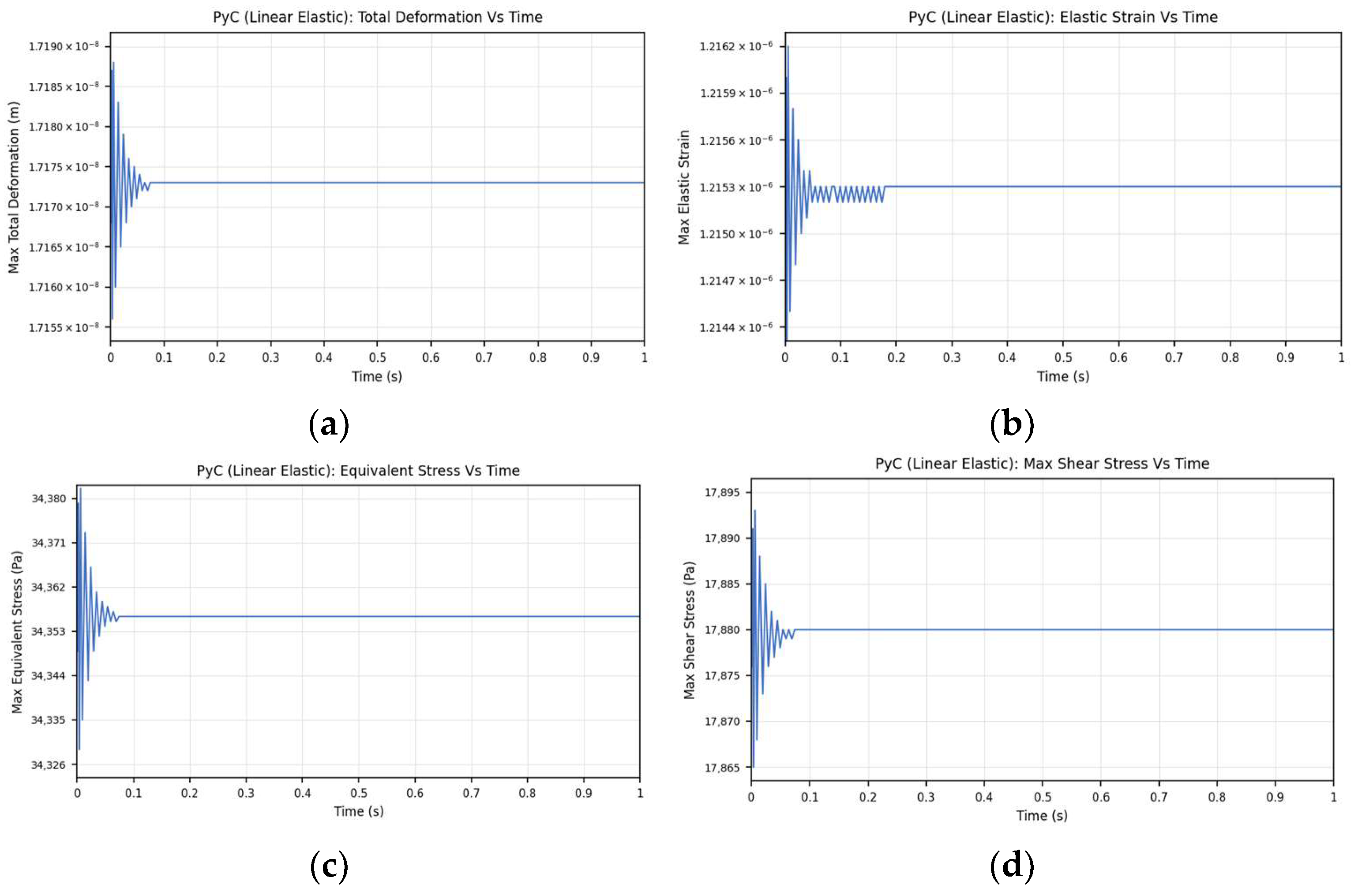
The pyrolytic carbon linear elastic model showed the most stable response among all cases. The time-history plots for total deformation (Figure 24a), equivalent elastic strain (Figure 24b), equivalent stress (Figure 24c), and maximum shear stress (Figure 24d) exhibited only very small oscillations at the beginning of the simulation, followed by rapid convergence to nearly constant values. This behavior is consistent with the extremely high stiffness of pyrolytic carbon and confirms its functionally rigid mechanical character. Because the material undergoes negligible deformation, the transient structural response remains weakly dynamic and reaches equilibrium quickly, with little evidence of sustained oscillatory behavior.
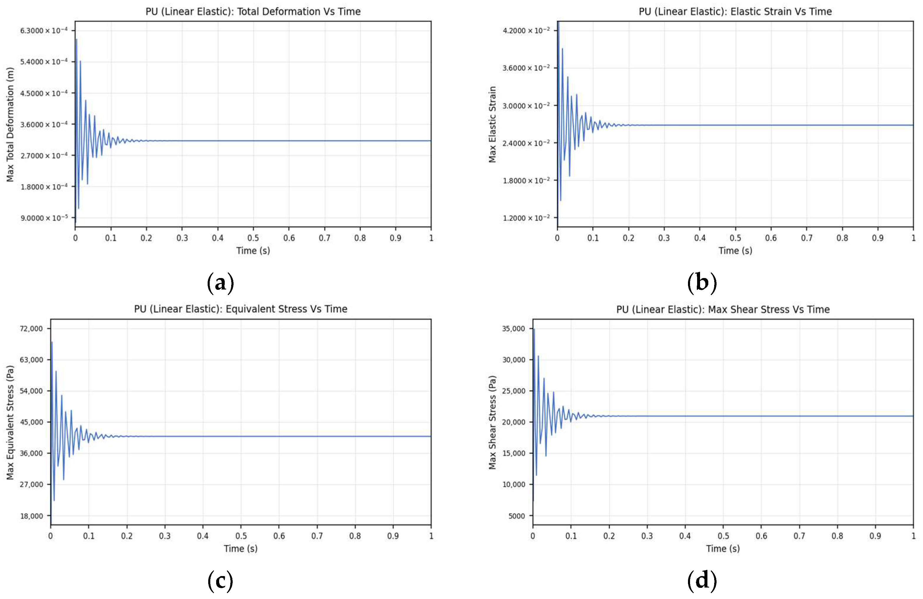
The polyurethane linear elastic model showed markedly larger transient amplitudes than pyrolytic carbon. In this case, total deformation (Figure 25a), equivalent strain (Figure 25b), equivalent stress (Figure 25c), and maximum shear stress (Figure 25d) all displayed pronounced oscillations during the early stage of the simulation before gradually approaching a stable response. The larger oscillatory amplitudes indicate greater compliance and stronger dynamic sensitivity of the leaflet structure under the applied loading. Compared with pyrolytic carbon, polyurethane therefore allows substantially greater deformation and stress redistribution, while still maintaining a bounded and stable response over the full cycle.
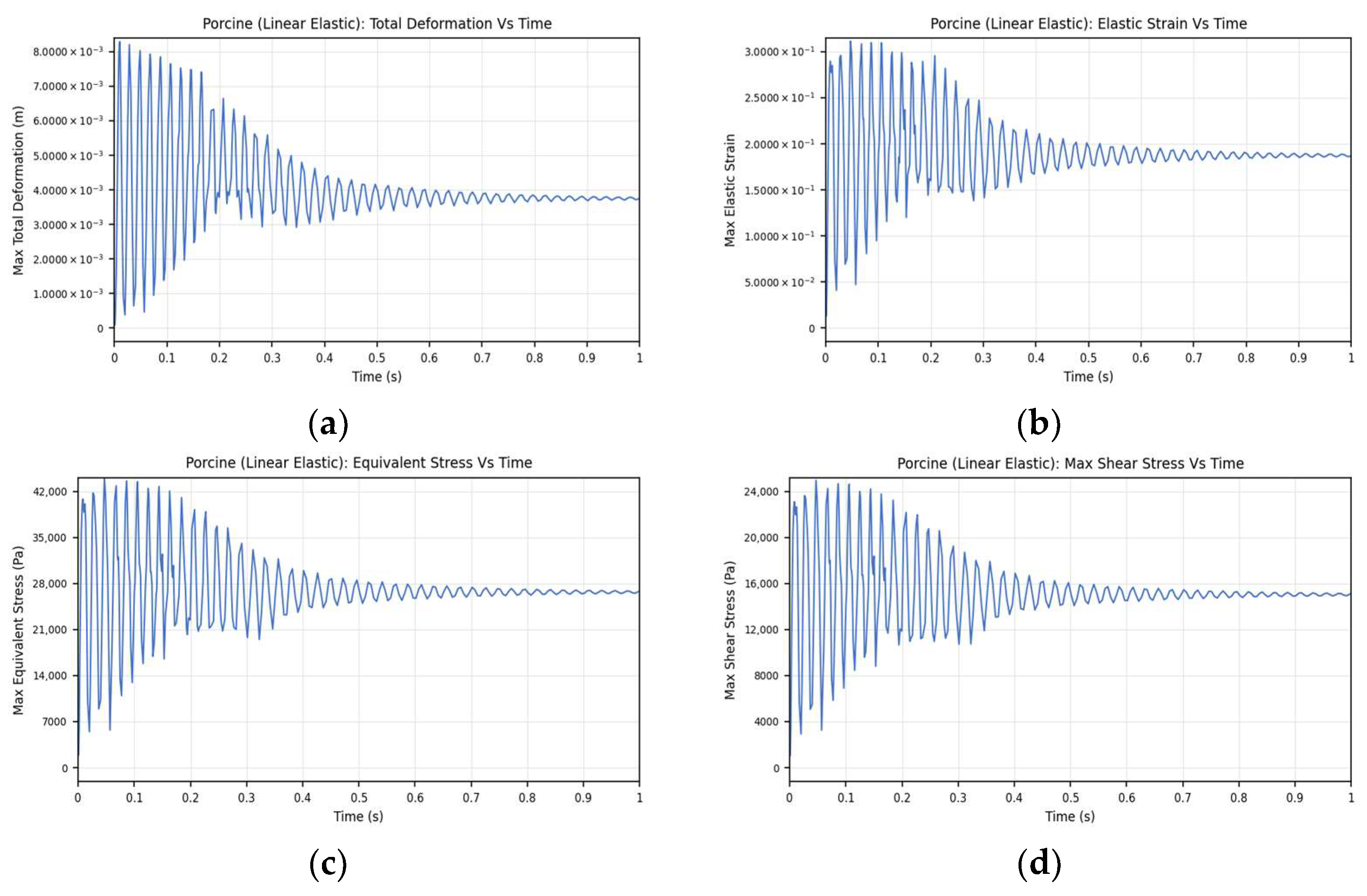
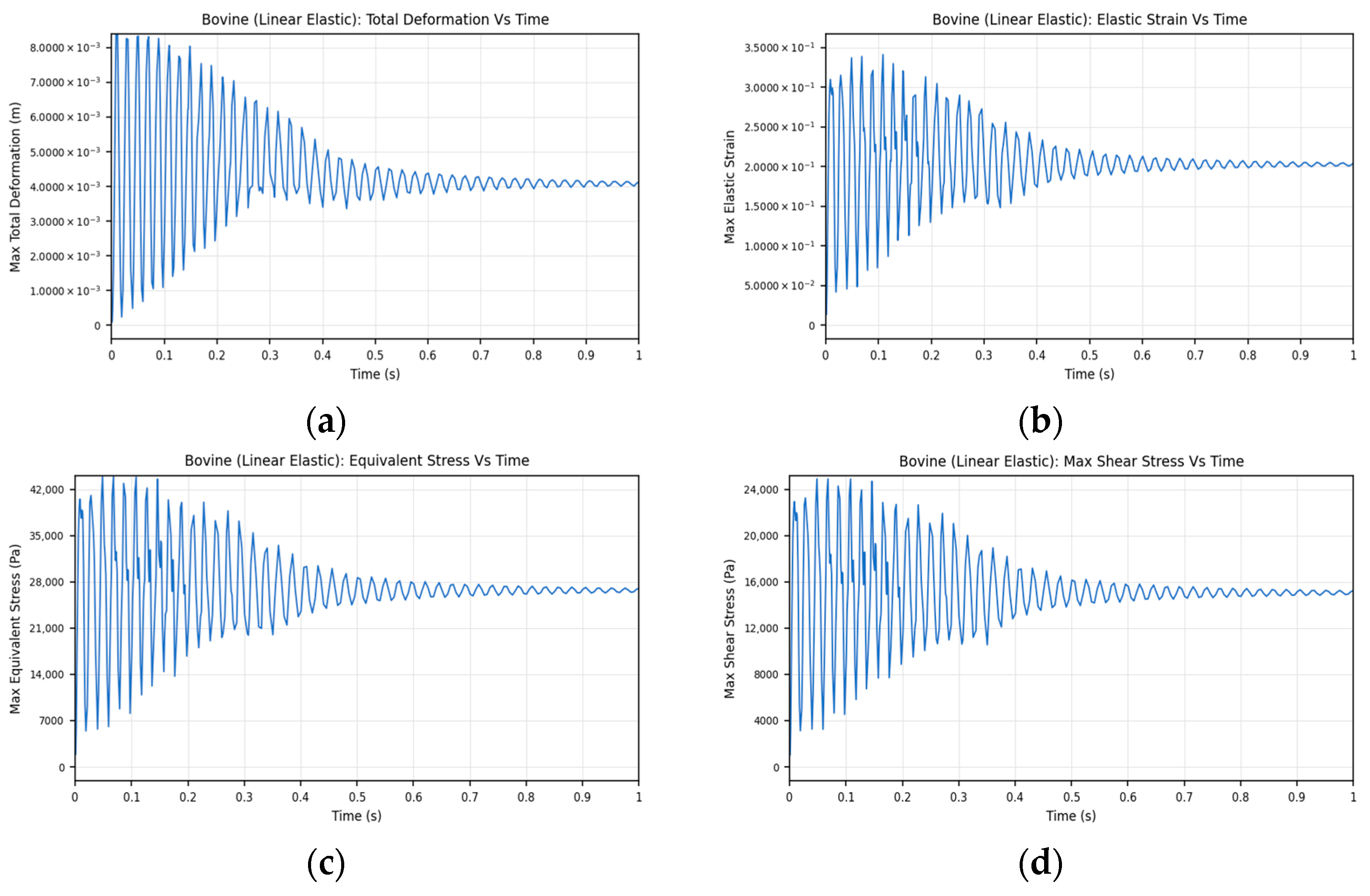
The porcine and bovine linear elastic tissue models exhibited larger transient amplitudes in deformation Figure 26a and Figure 27a) and strain (Figure 26b and Figure 27b) than the synthetic materials. Their time-history plots showed strong oscillatory behavior in the early portion of the simulation, followed by gradual decay toward a stabilized response. This indicates that the biological tissue models are substantially more compliant than pyrolytic carbon and polyurethane. The corresponding equivalent stress (Figure 26c and Figure 27c) and maximum shear stress curves (Figure 26d and Figure 27d) also displayed repeated transient peaks during the early loading period, reflecting the larger structural motion of the tissue leaflets and the resulting internal stress transfer. Among the linear elastic tissue cases, bovine tissue generally showed slightly higher stabilized deformation and strain levels than porcine tissue, which is consistent with the quantitative differences reported in Table 1.
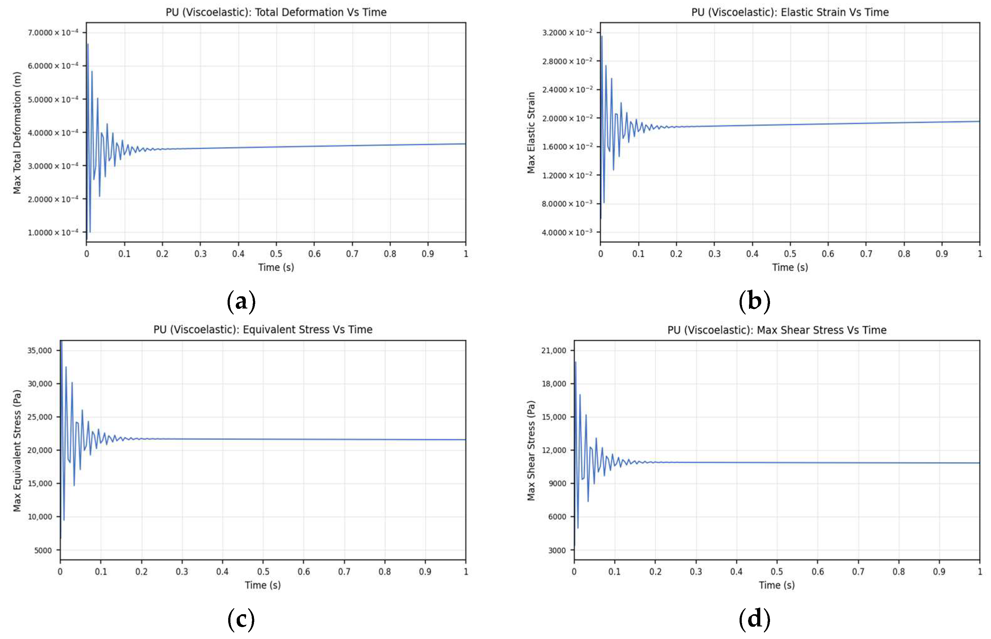
The viscoelastic polyurethane model showed a response pattern similar to the linear elastic polyurethane case, but with clearer damping and lower stabilized stress levels. The initial oscillations in deformation and strain (Figure 28a,b) were followed by a more rapid reduction in peak amplitudes for equivalent stress and maximum shear stress (Figure 28c,d), indicating the effect of time-dependent stress relaxation. In particular, the maximum shear stress and equivalent stress histories showed lower peaks than the linear elastic polyurethane model, which is consistent with the role of viscoelasticity in dissipating mechanical energy and reducing transient stress concentrations. This confirms that a viscoelastic representation is more appropriate for polyurethane than a purely linear elastic approximation when transient leaflet behavior is of interest.
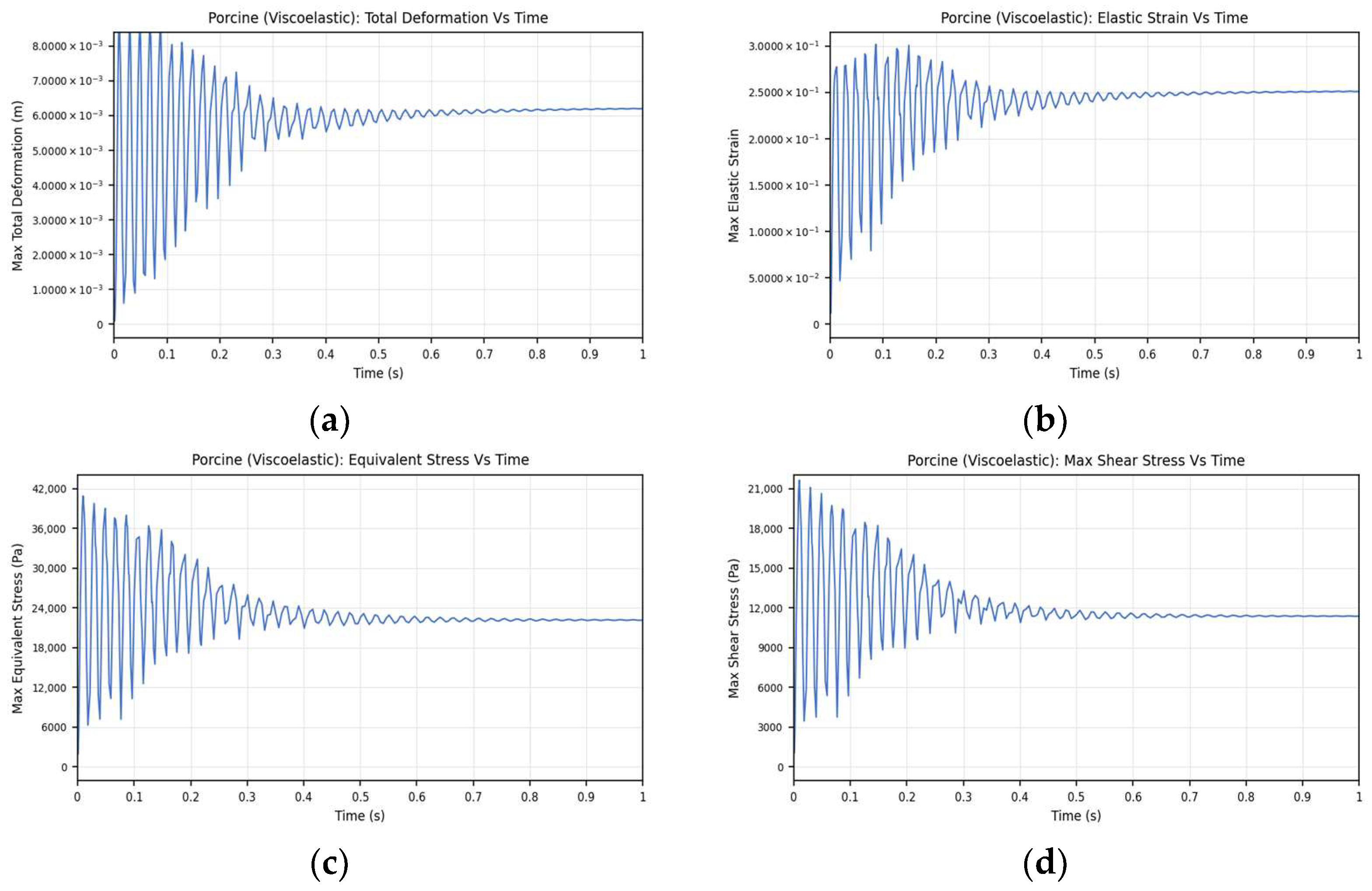
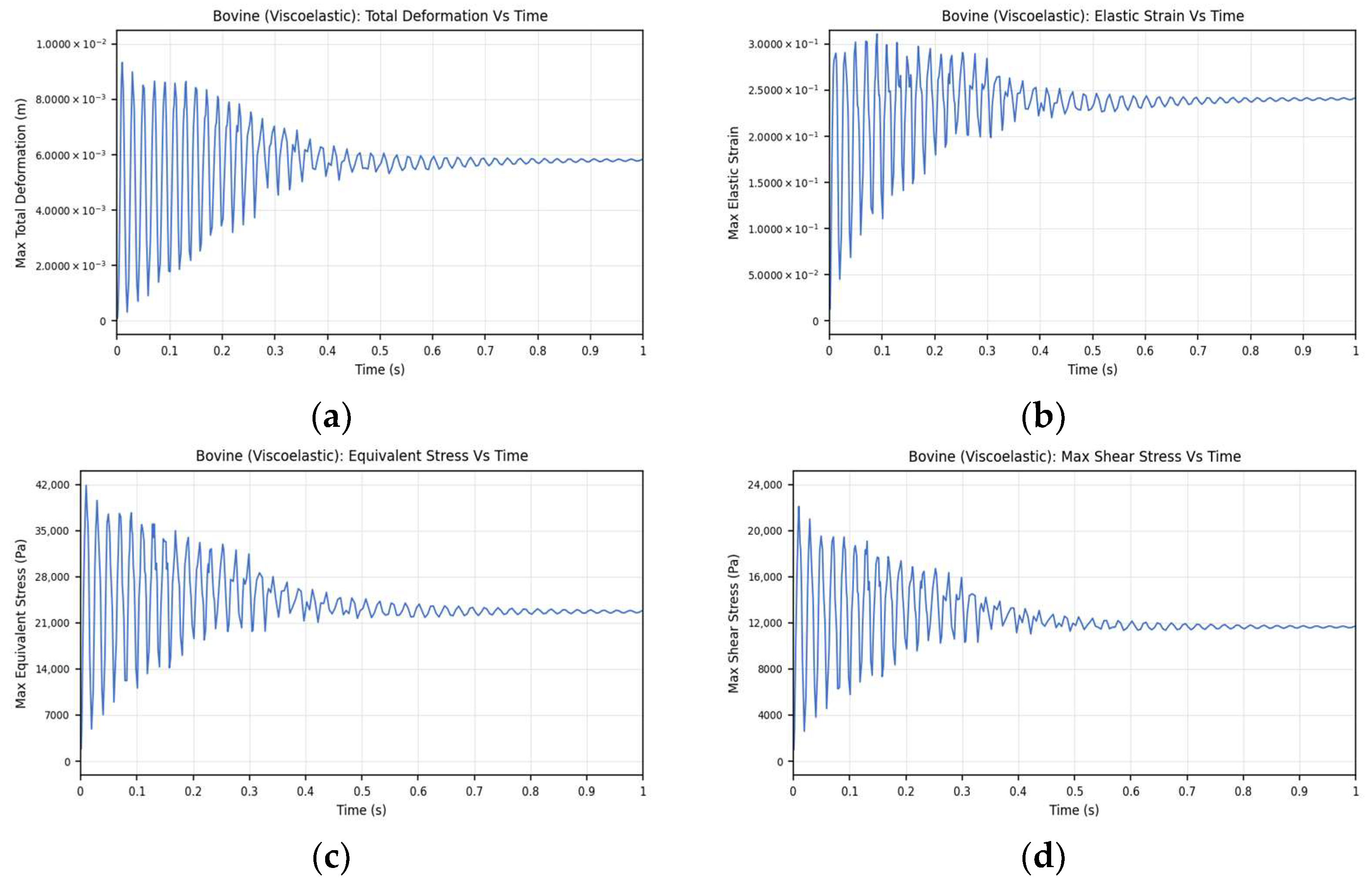
The viscoelastic porcine and bovine models showed continued oscillatory behavior, but the stress-related peaks were reduced relative to the corresponding linear elastic tissue models. This trend indicates that the addition of viscoelasticity introduces time-dependent damping and stress relaxation, which moderates transient stress transfer while preserving the overall compliant character of the biological tissues. The deformation (Figure 29a and Figure 30a) and strain histories (Figure 29b and Figure 30b) remained relatively large, confirming that these materials still undergo substantial motion during the cycle, but the reduced equivalent stress and maximum shear stress peaks (Figure 29c,d and Figure 30c,d) suggest a more distributed mechanical response. This behavior is consistent with the known stress-relaxation characteristics of soft biological tissues under cyclic loading.
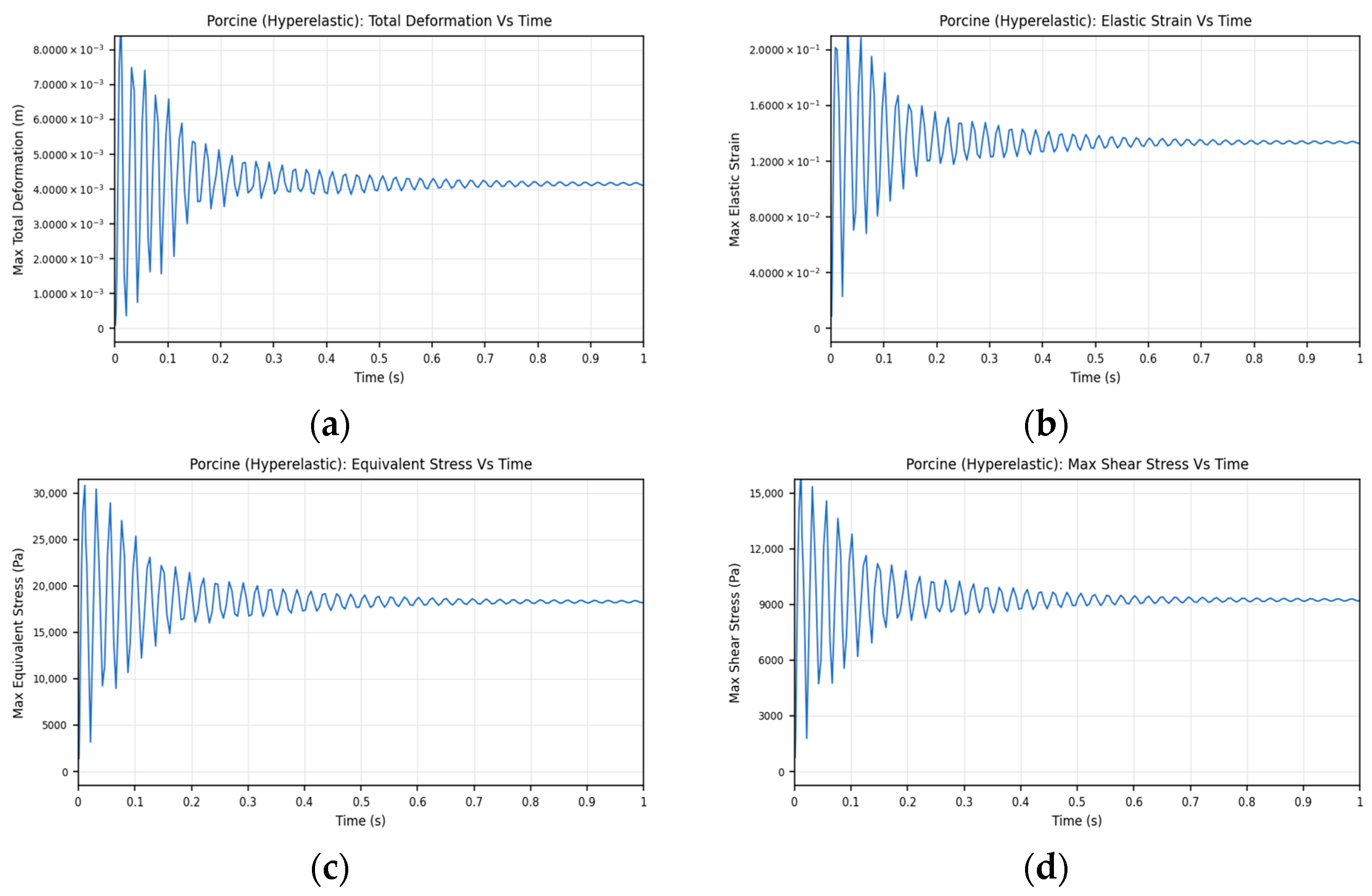
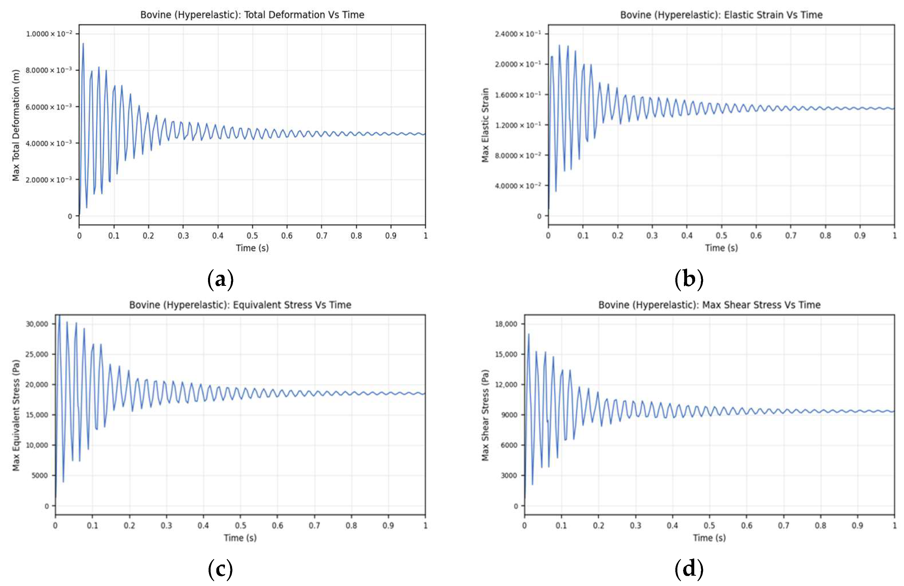
The hyperelastic porcine and bovine tissue models also exhibited pronounced early oscillations in deformation (Figure 31a and Figure 32a) and strain (Figure 31b and Figure 32b) followed by stabilization at lower stress levels than the linear elastic tissue models. In these cases, the equivalent stress (Figure 31c and Figure 32c) and maximum shear stress histories (Figure 31d and Figure 32d) demonstrated that the nonlinear constitutive behavior redistributed stress more effectively during deformation. Compared with the linear elastic tissue models, the hyperelastic formulations produced lower transient stress peaks and smoother stress evolution while maintaining substantial deformation capability. This confirms that hyperelastic constitutive laws better represent the nonlinear large-strain response of biological leaflet tissues and avoid the stress overprediction associated with purely linear elastic assumptions.
The maximum shear stress plots are particularly informative because they directly illustrate the temporal evolution of stress transfer during the transient simulation. Across all material models, maximum shear stress rose rapidly during the early response, oscillated as the structure adjusted to the imposed loading, and then approached a quasi-stable value. The amplitude of this oscillatory phase was smallest for pyrolytic carbon, intermediate for polyurethane, and largest for the tissue-based models. The viscoelastic and hyperelastic formulations generally reduced the stress peaks relative to the corresponding linear elastic cases, demonstrating that more realistic constitutive descriptions influence not only the magnitude of stress but also its time-dependent evolution.
Taken together, the transient plots confirm the trends identified from the contour maps and Table 1 while providing a more detailed interpretation of the dynamic structural response. Pyrolytic carbon behaves as a rigid material with rapid stabilization and negligible deformation; polyurethane shows intermediate compliance with material-dependent damping effects; and the biological tissues exhibit the greatest deformation and strain, with viscoelastic and hyperelastic formulations providing more favorable stress redistribution than linear elastic models. These time-history results therefore strengthen the interpretation of Section 3.1 by showing how the important physical observables evolve throughout the computational cycle rather than only at isolated states.

3.2. Computational Fluid Dynamics

3.2.1. Velocity Distribution and Flow Characteristics

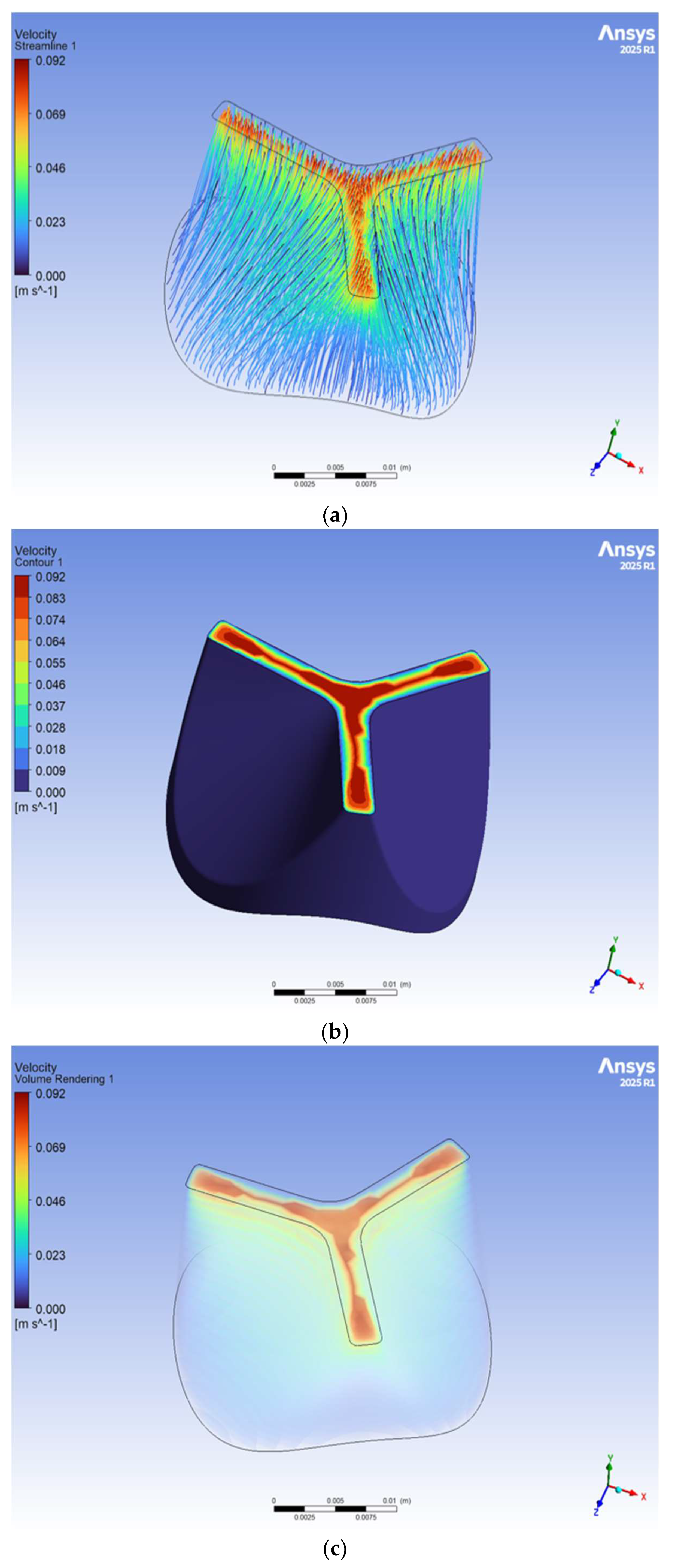
The velocity field within the fixed rigid tricuspid valve geometry demonstrated a well-defined jet formation through the valve opening, as shown in Figure 33a–d. The streamline visualization in Figure 33a revealed that the fluid accelerates as it passes through the valve orifice and forms a concentrated central jet extending downstream into the ventricular chamber. The maximum velocity magnitude observed was approximately 0.092 m/s, as indicated by the velocity scale. The streamlines remain aligned in the flow direction, confirming stable forward flow through the rigid valve geometry. Regions near the chamber walls exhibited significantly lower velocities, approaching zero due to the no-slip boundary condition.
The velocity contour shown in Figure 33b further confirms the presence of a high-velocity jet concentrated along the valve opening and leaflet edges. The highest velocity regions are localized at the narrow geometric constriction, where flow acceleration occurs due to conservation of mass and reduction in cross-sectional areas. The velocity decreased rapidly away from the jet region, indicating viscous dissipation and momentum diffusion into the surrounding fluid. The surrounding chamber region exhibits relatively low velocity magnitudes, highlighting the non-uniform velocity distribution imposed by the rigid valve geometry.
The three-dimensional velocity volume rendering shown in Figure 33c illustrates the spatial development of the velocity jet downstream of the valve opening. The jet expands gradually as it propagates into the chamber, indicating progressive momentum transfer from the high-velocity core to the surrounding slower fluid. This expansion reflects flow deceleration caused by geometric expansion and viscous effects. The highest velocity region remains confined to the effective orifice area and the immediate downstream region.
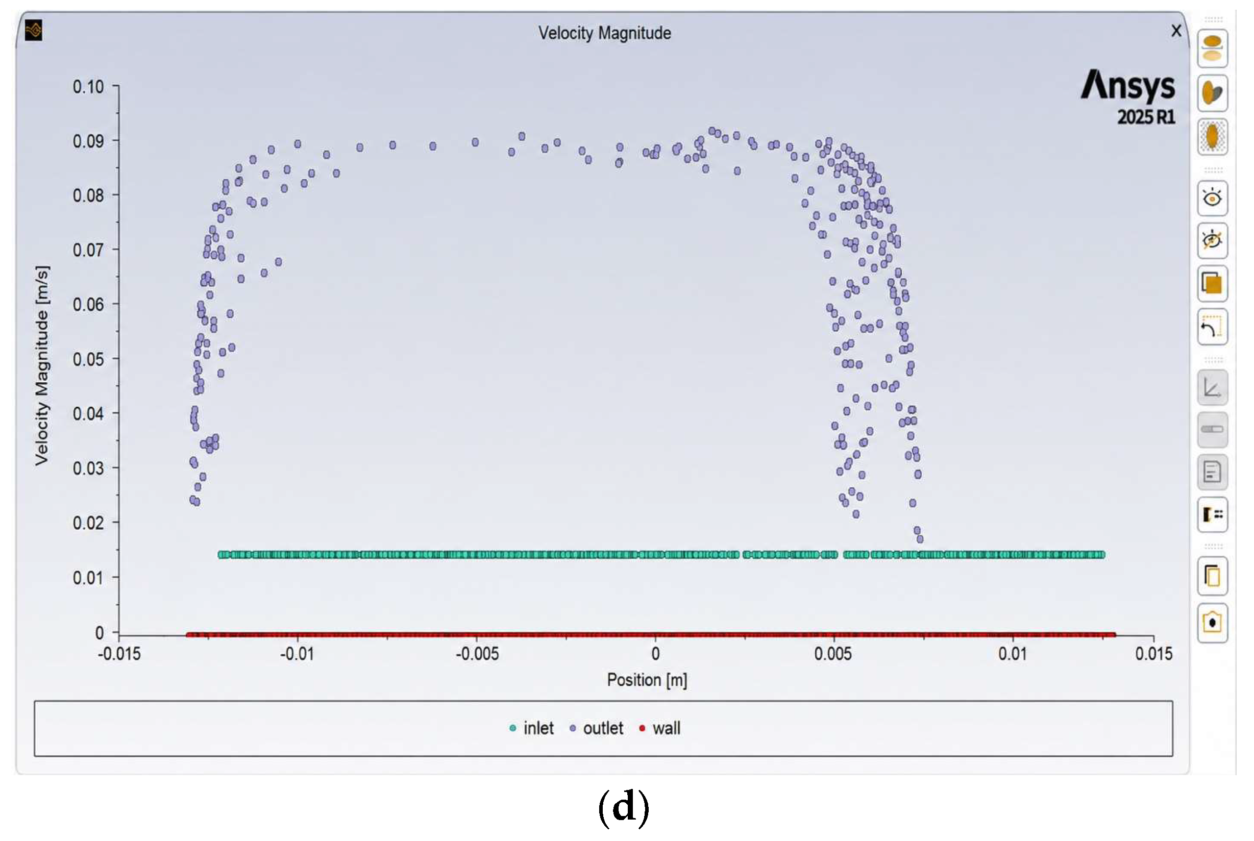
The velocity magnitude profile plotted as a function of spatial position in Figure 33d further quantifies the velocity distribution within the domain. The results show that peak velocity values of approximately 0.092 m/s occur near the valve opening, while velocity decreases significantly toward the chamber walls. The velocity near the walls approaches near-zero values due to the no-slip boundary condition. This velocity gradient between the high-velocity jet and the stationary wall regions resulted in shear layer formation and contributed to the development of downstream flow structures.
Overall, the velocity distribution demonstrates that the tricuspid valve geometry produces a well-defined central jet, with peak velocity occurring at the valve orifice and gradual velocity decay downstream and toward the chamber walls. These results confirm that the rigid valve geometry significantly influences the velocity field and governs the overall flow characteristics within the domain.

3.2.2. Vortex Formation and Flow Rotation

The vortex core regions identified within the tricuspid valve geometry were observed in Figure 34a,b. These vortex core visualizations reveal the presence of localized rotational flow structures primarily downstream of the valve opening and near the leaflet edges. The vortex cores were distributed along the chamber walls and in regions adjacent to the central velocity jet. The formation of these vortical structures indicates flow separation and recirculation caused by the sudden expansion of flow from the constricted valve orifice into the larger chamber volume. The velocity magnitude within the vortex regions ranged from near zero to approximately 0.092 m/s, with lower velocity regions corresponding to recirculation zones and higher velocity regions located near the jet boundary.
The Lambda-2 vortex identification criterion shown in Figure 34c further confirmed the presence of coherent vortex structures within the flow domain. Regions with negative Lambda-2 values represent stable vortex cores, indicating rotational flow behavior independent of pure shear deformation. The Lambda-2 distribution demonstrates that vortex formation occurs primarily near geometric discontinuities and regions of strong velocity gradients, particularly near leaflet edges and the downstream jet region. These vortical structures arise due to the interaction between the high-velocity jet and the surrounding slower fluid, resulting in rotational flow motion.
The velocity curl (vorticity magnitude) distribution shown in Figure 34d provides quantitative confirmation of rotational flow regions. The maximum vorticity magnitude observed was approximately 177 s−1, indicating strong rotational motion near the valve opening and leaflet boundaries. Elevated vorticity values were concentrated near the valve orifice and downstream regions where velocity gradients were highest. In contrast, lower vorticity values were observed in regions of slow flow near the chamber walls.
The presence of vortex structures and elevated vorticity confirms that the rigid tricuspid valve geometry induces rotational flow behavior due to geometric flow obstruction and jet interaction with the surrounding fluid. Since the valve is modeled as a fixed rigid structure, vortex formation is governed entirely by fluid dynamic effects and geometric constraints rather than structural deformation.
Overall, the results demonstrate that the tricuspid valve geometry promotes vortex formation, recirculation zones, and rotational flow structures downstream of the valve opening, which contribute to complex flow behavior within the chamber.

3.2.3. Pressure Distribution and Pressure Gradient

The static pressure distribution within the tricuspid valve geometry is shown in Figure 35a. The pressure contour reveals a clear pressure gradient across the valve opening, with maximum pressure values of approximately 14.7 Pa observed near the chamber wall and upstream regions, and minimum pressure values approaching 0 Pa near the valve opening and downstream regions. This pressure drop reflects the conversion of pressure energy into kinetic energy as fluid accelerates through the constricted valve orifice. The lowest pressure region was localized at the valve opening, corresponding to the region of highest velocity magnitude. The pressure drop of 14.7 Pa across the valve is consistent with low-resistance flow through a fully open prosthetic tricuspid valve. The velocity contours revealed a centrally located jet, which is characteristic of physiological tricuspid flow, with minimal stagnation zones observed near the leaflet bases.
The three-dimensional pressure volume rendering shown in Figure 35b further confirmed the spatial variation in pressure throughout the chamber. The pressure decreased progressively from the upstream region toward the valve opening and downstream regions. This smooth pressure transition indicates stable pressure-driven flow governed by geometric constraints of the rigid valve structure.
The pressure isosurface and streamline visualization shown in Figure 35c illustrate the relationship between pressure distribution and flow direction. The streamline patterns indicate that fluid accelerates through the central valve opening where pressure is lowest, and decelerates in the chamber region where pressure increases. This behavior is consistent with Bernoulli’s principle, where pressure decreases in regions of high velocity.
The pressure gradient contour shown in Figure 35d highlights regions of strong pressure variation near the leaflet edges and valve opening. The maximum pressure gradient magnitude observed was approximately 5629 Pa/m, indicating significant fluid acceleration in these regions. These high-pressure gradient regions correspond directly to the velocity jet formation and vortex generation regions observed in the velocity and vorticity results.
The cross-sectional flow visualization shown in Figure 35e further confirms the presence of a high-velocity central jet associated with low-pressure regions. The velocity vectors indicate that fluid accelerates rapidly through the valve opening, driven by the pressure difference across the valve.
The static pressure profile plotted as a function of spatial position, shown in Figure 35f, quantitatively confirms the pressure variation within the domain. The pressure was highest near the chamber wall and decreased toward the valve opening, with a total pressure drop of approximately 14.7 Pa across the valve. This pressure difference represents the driving force responsible for fluid acceleration through the rigid valve geometry.
Overall, the pressure distribution results demonstrate that the rigid tricuspid valve geometry produces a well-defined pressure gradient that drives fluid acceleration through the valve opening. The pressure drop across the valve corresponds directly to the velocity jet formation and vortex generation observed in the flow field, confirming the strong coupling between pressure and velocity distributions in the rigid valve configuration.

3.2.4. Instantaneous and Mean Wall Shear Stress Distribution

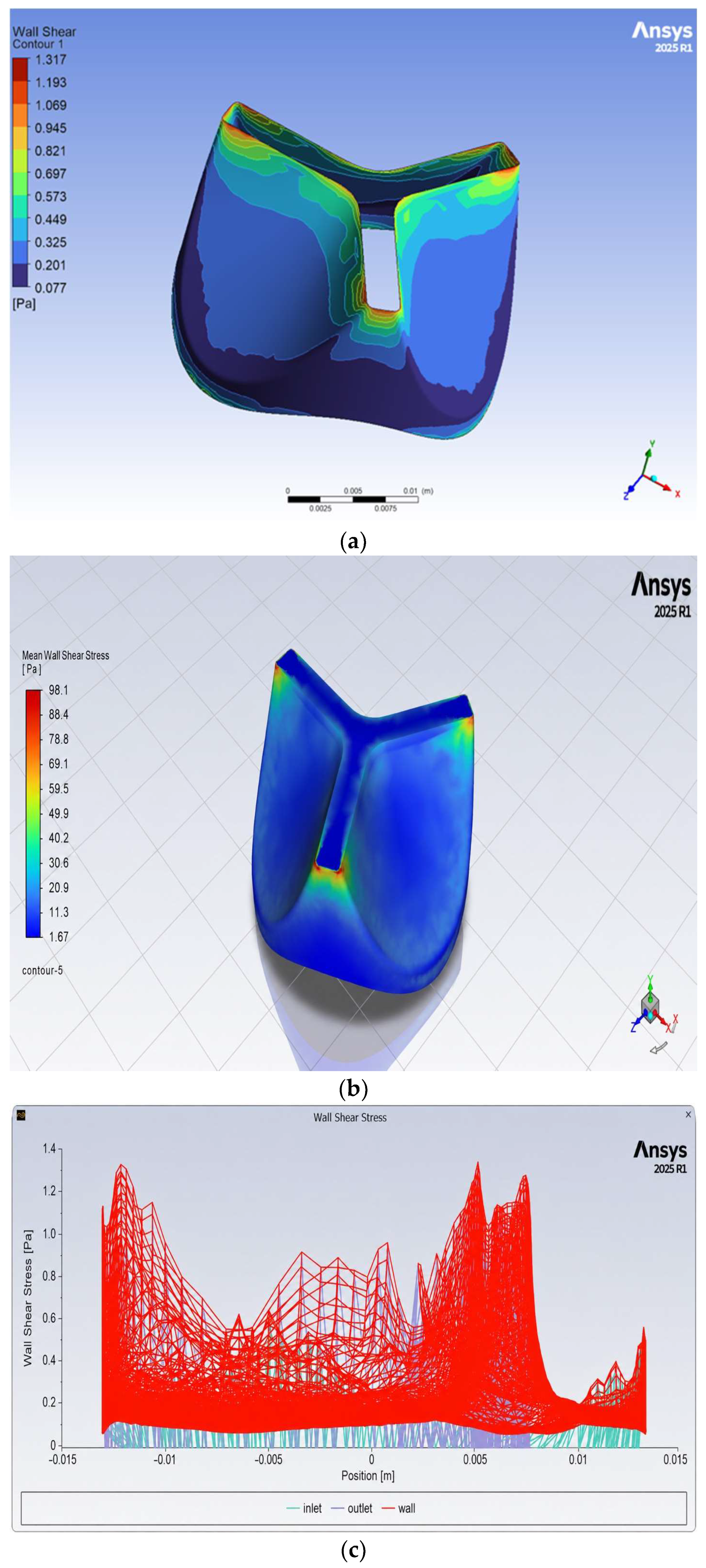
The instantaneous wall shear stress (WSS) distribution within the tricuspid valve geometry is shown in Figure 36a. The results demonstrate a non-uniform WSS distribution across the valve surface, with peak instantaneous WSS values reaching approximately 1.32 Pa, as indicated by the contour scale. The highest WSS values were concentrated near the leaflet edges and valve opening region, where the velocity gradients were greatest due to the acceleration of fluid through the constricted valve orifice. These regions correspond directly to the high-velocity jet and pressure gradient regions observed in the velocity and pressure distributions. In contrast, lower WSS values, approaching approximately 0.01 Pa, were observed in regions farther from the jet and near the chamber walls, where flow velocity was significantly lower.
The three-dimensional WSS visualization shown in Figure 36b further confirmed the spatial distribution of shear stress across the valve surface. Elevated WSS values were localized near the leaflet tips and valve opening, while the majority of the chamber surface experienced relatively low shear stress levels. This distribution reflects the influence of velocity gradients imposed by the rigid valve geometry and the no-slip boundary condition.
The instantaneous wall shear stress profile plotted as a function of spatial position in Figure 36c demonstrates significant spatial variability in WSS values across the valve surface. Peak WSS values were observed near the valve opening and leaflet edges, while lower values were observed in regions farther from the jet core. This variation confirms that the wall shear stress distribution is strongly dependent on the velocity gradient and flow acceleration through the valve.
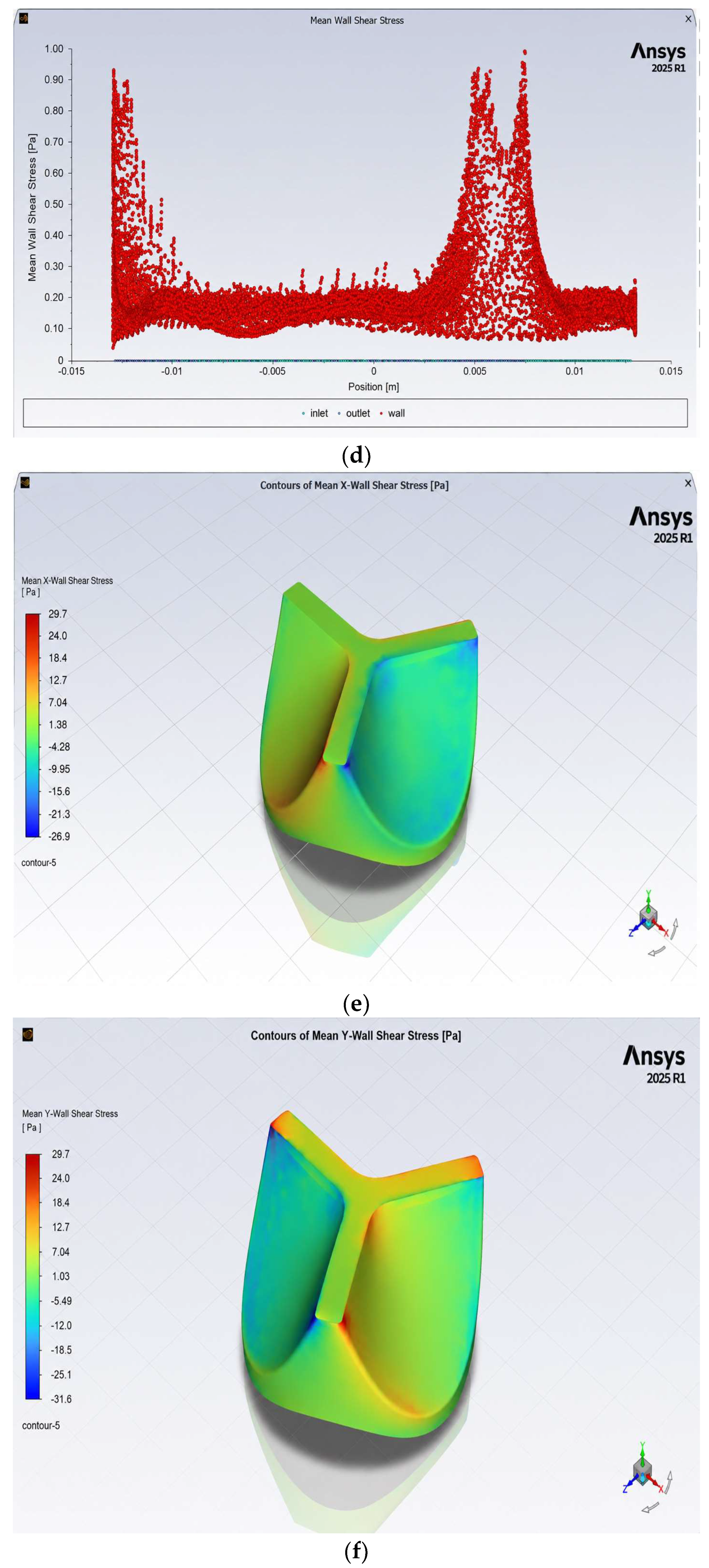
The mean wall shear stress distribution shown in Figure 36d further illustrates the spatial variation in shear stress across the valve surface. The mean WSS values ranged from approximately 0.02 Pa to 0.9 Pa, with peak values observed near the valve opening and leaflet boundaries. These regions correspond to areas of high velocity gradients and vortex formation identified in the velocity and vorticity results.
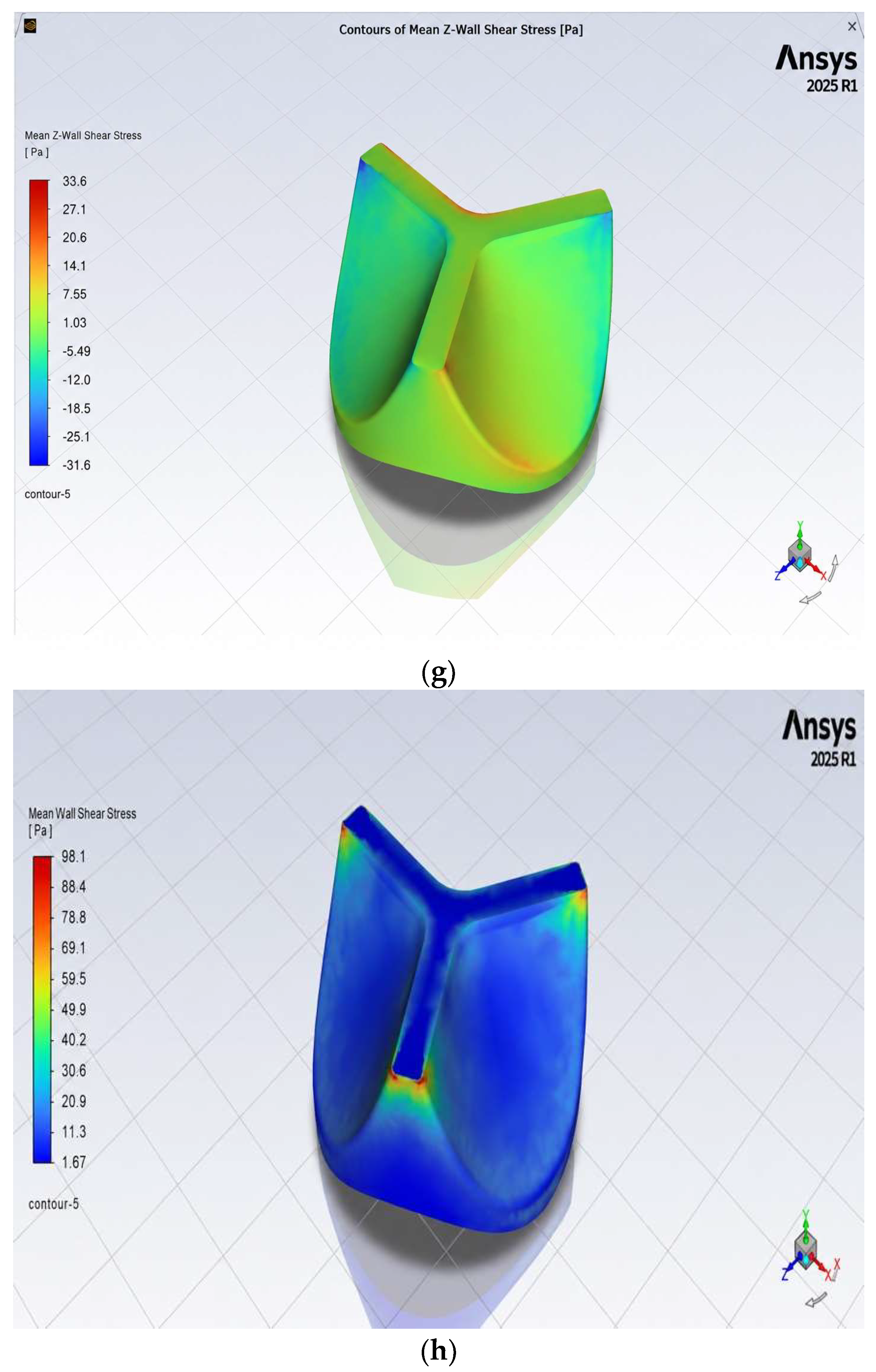
The directional components of mean wall shear stress are shown in Figure 36e–g. These results demonstrate that wall shear stress is distributed in multiple spatial directions due to the three-dimensional nature of the flow field. The magnitude and direction of shear stress varied across the valve surface, with higher values observed near geometric transition regions and lower values observed in regions of slower flow.
The mean wall shear stress contour shown in Figure 36h confirms that elevated shear stress values were concentrated near the valve opening and leaflet edges, while lower values were observed across the chamber surface. This distribution indicates that the rigid tricuspid valve geometry produces localized regions of elevated shear stress associated with the velocity jet and flow acceleration.
Overall, the CFD simulations demonstrated that the valve geometry generates a well-defined central jet with peak velocity of approximately 0.092 m/s, accompanied by localized vortex formation and moderate wall shear stress levels. The maximum vorticity magnitude reached approximately 177 s−1, while peak instantaneous wall shear stress was approximately 1.32 Pa near the leaflet edges. These results indicate that valve geometry strongly influences flow acceleration, recirculation zones, and shear stress distribution within the tricuspid valve domain.

4. Discussion

The selection of constitutive models in this study reflects the inherent physical hierarchies of the materials. While linear elasticity is sufficient for the functionally rigid PyC, synthetic polymers like PU require viscoelastic parameters to capture the hysteretic damping essential for prosthetic longevity. However, for biological xenografts, the inclusion of hyperelasticity is mandatory to replicate the ‘toe-region’ mechanics. Our results demonstrate that neglecting hyperelasticity in porcine and bovine models leads to a significant divergence in peak stress predictions, whereas for PU, the viscoelastic relaxation is the dominant driver of transient structural stability.

4.1. Structural Rigidity of Pyrolytic Carbon

The structural simulations demonstrated that pyrolytic carbon exhibits extremely small deformation under physiological loading conditions. In the present study, the maximum deformation observed for pyrolytic carbon was approximately 1.92 × 10⁻⁸ m, indicating extremely high structural stiffness. Mechanical heart valves fabricated from pyrolytic carbon are well known for their high durability and wear resistance, which has supported their continued clinical use over decades. The very high stiffness of pyrolytic carbon also means that the valve leaflets behave as functionally rigid components, resulting in negligible structural deformation under physiological loading. While this rigidity contributes to durability, it also limits the ability of the leaflets to absorb mechanical energy during the cardiac cycle and may promote non-physiological flow features associated with mechanical prosthetic valves [19,40,41].
The maximum von Mises stress obtained in this study for pyrolytic carbon was approximately 3.4 × 10⁴ Pa, which is comparable to stress magnitudes reported in numerical studies of mechanical heart valve components. Although such stress levels are well within the material strength limits, the extremely low strain energy observed in this study (2.59 × 10⁻¹² J) indicates minimal energy absorption during deformation. Previous studies have suggested that the rigid nature of mechanical valve materials may contribute to non-physiological stress transfer and increased thrombogenic potential in mechanical prosthetic valves [17,40,42,43].

4.2. Mechanical Compliance of Biological Valve Tissues

In contrast to pyrolytic carbon, the biological tissues (porcine and bovine) demonstrated significantly greater deformation and strain under identical loading conditions. The maximum deformation observed for porcine tissue was approximately 4.14 × 10⁻³ m, while bovine tissue exhibited slightly higher deformation of approximately 4.49 × 10⁻³ m. These deformation magnitudes reflect the inherently compliant nature of biological valve tissues, which consist primarily of collagen and elastin fibers arranged in anisotropic structures.
Experimental and computational studies of native and bioprosthetic valve tissues have reported similar mechanical behavior. Pericardial tissues used in bioprosthetic valves exhibit nonlinear and anisotropic deformation under physiological loading, primarily due to the collagen fiber architecture within the tissue. The collagen network enables the leaflet to undergo large deformation while redistributing mechanical stress across the tissue surface, thereby improving structural compliance during valve opening and closing. Previous biomechanical investigations of pericardial valve tissues have confirmed that this collagen-dominated structure leads to nonlinear stress–strain behavior and directional mechanical properties that are essential for physiological valve function [32,44].
In the present study, the equivalent stresses observed for biological tissues were approximately 1.68 × 10⁴ Pa for porcine tissue and 1.70 × 10⁴ Pa for bovine tissue, which are considerably lower than those observed in pyrolytic carbon. This reduction in stress magnitude results from the ability of biological tissues to undergo large deformation while redistributing loads across the leaflet surface.
Furthermore, the maximum strain values obtained in this study (0.125 for porcine tissue and 0.133 for bovine tissue) fall within the range reported in experimental investigations of heart valve tissues. Previous studies have demonstrated that native valve leaflets can experience large strain without structural failure due to their collagen fiber architecture and nonlinear stress–strain response [45].
The strain energy results further confirm the energy-absorbing capability of biological tissues [45]. The strain energy observed in this study for porcine and bovine tissues (~2 × 10⁻⁷ J) was several orders of magnitude higher than that observed in pyrolytic carbon. Such energy absorption allows biological tissues to function as mechanical dampers during valve motion, which helps maintain physiological valve function and reduces stress concentration. However, despite their favorable mechanical compliance, bioprosthetic tissues are susceptible to structural valve deterioration (SVD). Clinical studies have shown that bioprosthetic valves typically have a lifespan of 10–15 years, primarily due to tissue calcification and mechanical fatigue.

4.3. Polyurethane as a Polymeric Alternative

Polyurethane exhibited intermediate mechanical behavior between rigid pyrolytic carbon and compliant biological tissues. The maximum deformation observed for polyurethane in this study was approximately 3.64 × 10⁻⁴ m, which is significantly greater than that of pyrolytic carbon but lower than that of biological tissues.
The maximum von Mises stress observed in polyurethane reached approximately 2.16 × 10⁴ Pa, indicating that the material experiences moderate stress levels under loading conditions. These results suggest that polyurethane possesses sufficient flexibility to redistribute loads while maintaining greater structural stability than natural tissues.
Polymeric heart valves have been extensively investigated as potential alternatives to both mechanical and bioprosthetic valves. A comprehensive review by Li et al. (2019) reported that polyurethane-based heart valves can combine the durability of synthetic materials with improved hemodynamic performance compared with rigid mechanical valves [46].
The strain energy observed for polyurethane ranged from 2.16 × 10⁻⁸ J to 4.05 × 10⁻⁸ J, indicating moderate energy absorption compared with biological tissues. This indicates that polyurethane can absorb mechanical energy during deformation while maintaining structural integrity. Such properties suggest that polymeric materials may provide a balance between durability and physiological compliance.
Because long-term durability is central to prosthetic valve selection, a literature-based comparison of representative lifespan information for the four material classes considered in this study is provided in Table 2. Pyrolytic carbon and clinically established bioprosthetic tissues have reported long-term service histories, whereas polyurethane-based prosthetic valves remain primarily in the experimental and preclinical stage; therefore, a definitive long-term clinical lifespan for polyurethane prosthetic heart valves has not yet been established in the available clinical literature.
As shown in Table 2, polyurethane should therefore be interpreted as a promising candidate material with favorable fatigue resistance and flexibility, but not yet as a material with a proven long-term clinical lifespan comparable to pyrolytic carbon or established bioprosthetic tissues [13,15,16].

4.4. Hemodynamic Characteristics

The computational fluid dynamics analysis revealed the formation of a central velocity jet through the valve orifice with a peak velocity of approximately 0.092 m/s. The presence of this central jet is typical in prosthetic heart valves, where fluid accelerates through a constricted orifice before expanding into the downstream chamber. The CFD results obtained in the present study were interpreted against literature-reported hemodynamic characteristics of prosthetic heart valves rather than as stand-alone experimental validation. Previous studies have shown that forward jet formation through the valve orifice, downstream recirculation, localized vortex structures, and elevated wall shear stress near leaflet edges are common features of prosthetic-valve flow fields [17,19,20]. In this context, the central jet, localized vorticity, pressure drop, and non-uniform wall shear stress predicted in the present rigid tricuspid model are consistent with established computational and experimental descriptions of heart-valve hemodynamics [17,19,20]. However, because the present CFD model used a rigid, fully open valve configuration, these comparisons should be interpreted as supporting the physical plausibility of the simulated flow field rather than as full validation of device performance, which would require direct in vitro, ex vivo, or fluid–structure interaction-based comparison [22,23].
The simulations also revealed the formation of localized vortex structures downstream of the valve opening, with a maximum vorticity magnitude of approximately 177 s−1. Similar flow structures have been observed in previous hemodynamic studies of prosthetic valves, where jet expansion and sudden geometric changes induce recirculation regions. Previous investigations have demonstrated that vortex structures, flow separation, and recirculation regions in prosthetic heart valves can promote platelet activation and blood damage because these flow features are associated with elevated shear stresses [47].
Experimental and numerical studies of mechanical heart valves have further shown that flow-induced shear exposure increases thrombogenic potential [48]. The wall shear stress analysis in the present study revealed peak instantaneous WSS values of approximately 1.32 Pa, concentrated near the leaflet edges and valve opening. These regions correspond to areas of strong velocity gradients generated by the high-velocity jet. Previous research has shown that elevated shear stress regions may contribute to platelet activation and thrombotic complications in prosthetic heart valves.

4.5. Implications for Prosthetic Valve Material Selection

The structural and hemodynamic results highlight the importance of balancing durability and physiological compliance when selecting materials for prosthetic valve design.
Pyrolytic carbon demonstrated extremely low deformation and high structural rigidity, which explains the excellent durability of mechanical heart valves. However, the rigid mechanical behavior may contribute to elevated stress transfer and increased thrombogenic risk.
Biological tissues such as porcine and bovine pericardium demonstrated significantly greater compliance and energy absorption. These characteristics contribute to improved physiological behavior and lower stress concentrations but are associated with limited long-term durability.
Polyurethane demonstrated intermediate mechanical properties, combining moderate flexibility with improved structural stability. These findings suggest that polymeric heart valves may provide a promising compromise between mechanical durability and physiological compliance.
Overall, the results of this study suggest that optimal prosthetic valve design requires careful balancing of structural stiffness, energy absorption, and hemodynamic performance to achieve long-term durability and physiological compatibility.

4.6. Study Limitations

While the present study provides useful comparative insight into tricuspid valve mechanics and flow behavior, several limitations should be acknowledged. First, the CFD analysis treated the valve as a rigid, fully open structure, so leaflet motion was not coupled to the fluid field. Recent heart-valve FSI studies show that including leaflet motion can change predicted velocity patterns, stress transmission, and oscillatory leaflet behavior, which means the present rigid-wall assumption is a simplification [49]. Also, previous studies have shown that fully coupled fluid–structure interaction (FSI) simulations provide a more realistic representation of valve motion and flow–structure feedback in heart valve systems [50]. Although the structural analysis showed that leaflet deformation depends strongly on material properties, the CFD study was intentionally performed using a rigid, fully open valve configuration to isolate geometry-driven hemodynamic behavior. As a result, the structural and CFD analyses are complementary but not fully coupled. Material-specific leaflet deformation would be expected to affect the effective orifice area, local jet development, recirculation patterns, pressure drop, and wall shear stress. Accordingly, the present CFD results should be interpreted as a simplified reference case, while future fluid–structure interaction simulations are needed to quantify the direct influence of material-dependent deformation on flow behavior.
Second, the current structural framework used simplified constitutive descriptions for some materials and did not explicitly account for anisotropic leaflet fiber architecture. Recent studies have shown that leaflet anisotropy and material extensibility can substantially influence deformation, stent or leaflet motion, and local stress fields in bioprosthetic or atrioventricular valve simulations [51].
Third, blood was modeled as a Newtonian fluid, which is a common approximation in valve CFD, but recent work suggests that non-Newtonian rheology can alter predicted hemodynamic magnitudes, including recirculation strength and wall shear stress, especially in regions of separated or disturbed flow [52].
Finally, the study used a single idealized valve geometry and one set of loading and boundary conditions. As a result, the conclusions are most appropriate as a controlled comparative analysis rather than a patient-specific prediction. The present results therefore provide material-level and constitutive-model trends, but not a direct surrogate for in vivo clinical performance.

4.7. Future Work

Future work should extend the present framework to fully coupled fluid–structure interaction (FSI) simulations so that leaflet motion and blood flow can be solved simultaneously. Recent validated FSI studies indicate that this approach is better suited for resolving transient leaflet kinematics and flow-structure feedback in valve systems [23].
A second important direction is the use of anisotropic hyperelastic constitutive models for porcine and bovine tissues. Recent studies on leaflet extensibility and bioprosthetic anisotropy suggest that incorporating directional tissue mechanics would improve the physiological realism of the predicted deformation and stress fields [51].
Future studies should also examine non-Newtonian blood rheology in the tricuspid configuration, especially because disturbed flow regions were observed near the leaflet edges and downstream vortex zones in the present work. Recent comparative studies show that Newtonian and non-Newtonian models can produce different magnitudes of WSS, recirculation, and other hemodynamic metrics, even when general flow patterns remain similar [53].
In addition, the role of advanced polymeric valve materials deserves further investigation. Recent reviews and computational studies continue to identify polymeric heart valves as promising candidates because they may offer a balance between compliance and durability, although long-term fatigue and clinical translation remain open questions [54].
Finally, future research should incorporate patient-specific geometries and experimental validation, including in vitro flow-loop testing and material characterization, to strengthen the translational relevance of the computational findings. Recent validated computational valve studies support this direction [23].

5. Conclusions

This study presents a comprehensive computational investigation of the structural and hemodynamic performance of four prosthetic valve materials: pyrolytic carbon, polyurethane, porcine tissue, and bovine tissue, within a tricuspid valve geometry. Transient structural simulations and computational fluid dynamics analyses were conducted to evaluate the influence of material stiffness and constitutive behavior on valve deformation, stress distribution, strain energy absorption, and flow characteristics.
The structural analysis demonstrated that pyrolytic carbon exhibited extremely low deformation and strain due to its high stiffness, confirming its excellent structural stability and durability. However, the limited strain energy absorption observed for pyrolytic carbon indicates reduced mechanical compliance compared with more flexible materials. In contrast, biological tissues such as porcine and bovine pericardium showed significantly greater deformation and strain, along with higher strain energy values, reflecting their ability to absorb mechanical loads and redistribute stresses more effectively during the cardiac cycle. Polyurethane demonstrated intermediate mechanical behavior, combining moderate deformation with relatively balanced stress levels, suggesting its potential as a promising polymeric alternative for prosthetic valve design.
The computational fluid dynamics analysis revealed that the rigid tricuspid valve geometry produced a well-defined central velocity jet with a peak velocity of approximately 0.092 m/s, accompanied by localized vortex formation and pressure gradients near the valve opening. The resulting wall shear stress distribution was highly non-uniform, with peak instantaneous values of approximately 1.32 Pa concentrated near the leaflet edges and regions of strong velocity gradients. These hemodynamic features highlight the significant influence of valve geometry on flow acceleration, vortex generation, and shear stress distribution.
Overall, the results indicate that material stiffness plays a critical role in determining the mechanical and hemodynamic performance of prosthetic valves. Rigid materials such as pyrolytic carbon provide superior structural durability but limited compliance, whereas biological tissues offer improved flexibility and energy absorption but reduced long-term durability. Polyurethane exhibits balanced mechanical behavior and may represent a promising compromise between durability and physiological compliance. These findings contribute to the understanding of how material selection influences prosthetic valve biomechanics and may support the development of improved tricuspid valve replacement designs.
Future studies incorporating fluid–structure interaction simulations, anisotropic tissue models, and patient-specific geometries will further enhance the accuracy of computational predictions and provide deeper insight into prosthetic valve performance under physiological conditions.

Author Contributions

Conceptualization, S.N. and T.G.; methodology, S.N. and T.G.; software, S.N.; validation, S.N. and T.G.; formal analysis, S.N. and T.G.; investigation, S.N. and T.G.; resources, S.N. and T.G.; data curation, S.N. and T.G.; writing—original draft preparation, S.N.; writing—review and editing, S.N. and T.G.; visualization, S.N. and T.G.; supervision, S.N. and T.G.; project administration, T.G. All authors have read and agreed to the published version of the manuscript.

Funding

This research received no external funding.

Data Availability Statement

Data are contained within the article.

Conflicts of Interest

The authors declare no conflicts of interest.

Appendix A. Additional Figures of Structural Analysis of Tricuspid Heart Valve

Pyrolytic Carbon (Linear Elastic)
Figure A1. Total deformation.
Designs 10 00057 g0a1
Figure A2. Maximum Principal Stress.
Designs 10 00057 g0a2
Figure A3. Equivalent Stress.
Designs 10 00057 g0a3
Figure A4. Maximum Shear Stress.
Designs 10 00057 g0a4
Figure A5. Equivalent Elastic Strain.
Designs 10 00057 g0a5
Figure A6. Strain Energy.
Designs 10 00057 g0a6
Polyurethane (Vicoelastic)
Figure A7. Total deformation.
Designs 10 00057 g0a7
Figure A8. Equivalent Stress.
Designs 10 00057 g0a8
Figure A9. Maximum Principal Stress.
Designs 10 00057 g0a9
Figure A10. Maximum Shear Stress.
Designs 10 00057 g0a10
Figure A11. Equivalent Elastic Strain.
Designs 10 00057 g0a11
Figure A12. Strain Energy.
Designs 10 00057 g0a12
Polyurethane (linear elastic)
Figure A13. Total deformation.
Designs 10 00057 g0a13
Figure A14. Equivalent Stress.
Designs 10 00057 g0a14
Figure A15. Maximum Principal Stress.
Designs 10 00057 g0a15
Figure A16. Maximum Shear Stress.
Designs 10 00057 g0a16
Figure A17. Strain Energy.
Designs 10 00057 g0a17
Figure A18. Equivalent Elastic Strain.
Designs 10 00057 g0a18
Porcine linear elastic
Figure A19. Total Deformation.
Designs 10 00057 g0a19
Figure A20. Maximum Principal Stress.
Designs 10 00057 g0a20
Figure A21. Equivalent Stress.
Designs 10 00057 g0a21
Figure A22. Maximum Shear Stress.
Designs 10 00057 g0a22
Figure A23. Equivalent Elastic Strain.
Designs 10 00057 g0a23
Figure A24. Strain Energy.
Designs 10 00057 g0a24
Porcine (viscoelastic)
Figure A25. Total deformation.
Designs 10 00057 g0a25
Figure A26. Maximum Principal Stress.
Designs 10 00057 g0a26
Figure A27. Maximum Shear Stress.
Designs 10 00057 g0a27
Figure A28. Equivalent Stress.
Designs 10 00057 g0a28
Figure A29. Equivalent Elastic Strain.
Designs 10 00057 g0a29
Figure A30. Strain Energy.
Designs 10 00057 g0a30
Porcine (Hyperelastic)
Figure A31. Total deformation.
Designs 10 00057 g0a31
Figure A32. Maximum Shear Stress.
Designs 10 00057 g0a32
Figure A33. Maximum Principal Stress.
Designs 10 00057 g0a33
Figure A34. Equivalent Stress.
Designs 10 00057 g0a34
Figure A35. Equivalent Elastic Strain.
Designs 10 00057 g0a35
Figure A36. Strain Energy.
Designs 10 00057 g0a36
Bovine (linear elastic)
Figure A37. Total deformation.
Designs 10 00057 g0a37
Figure A38. Equivalent Stress.
Designs 10 00057 g0a38
Figure A39. Maximum Principal Stress.
Designs 10 00057 g0a39
Figure A40. Maximum Shear Stress.
Designs 10 00057 g0a40
Figure A41. Equivalent Elastic Strain.
Designs 10 00057 g0a41
Figure A42. Strain Energy.
Designs 10 00057 g0a42
Bovine (visco elastic)
Figure A43. Total deformation.
Designs 10 00057 g0a43
Figure A44. Equivalent Stress.
Designs 10 00057 g0a44
Figure A45. Maximum Principal Stress.
Designs 10 00057 g0a45
Figure A46. Maximum Shear Stress.
Designs 10 00057 g0a46
Figure A47. Equivalent Elastic Strain.
Designs 10 00057 g0a47
Figure A48. Strain Energy.
Designs 10 00057 g0a48
Bovine (Hyperelastic)
Figure A49. Total deformation.
Designs 10 00057 g0a49
Figure A50. Equivalent Stress.
Designs 10 00057 g0a50
Figure A51. Maximum Principal Stress.
Designs 10 00057 g0a51
Figure A52. Maximum Shear Stress.
Designs 10 00057 g0a52
Figure A53. Equivalent Elastic Strain.
Designs 10 00057 g0a53
Figure A54. Strain Energy.
Designs 10 00057 g0a54

References

  1. Oliveira, D.C.; Oliveira, C.G.C. The Forgotten, Not Studied or Not Valorized Tricuspid Valve: The Transcatheter Revolution Is Coming. Cardiol. Res. 2019, 10, 199–206. [Google Scholar] [CrossRef] [Scilit]
  2. Zack, C.J.; Fender, E.A.; Chandrashekar, P.; Reddy, Y.N.V.; Bennett, C.E.; Stulak, J.M.; Miller, V.M.; Nishimura, R.A. National Trends and Outcomes in Isolated Tricuspid Valve Surgery. J. Am. Coll. Cardiol. 2017, 70, 2953–2960. [Google Scholar] [CrossRef] [Scilit] [PubMed]
  3. Nath, J.; Foster, E.; Heidenreich, P.A. Impact of Tricuspid Regurgitation on Long-Term Survival. J. Am. Coll. Cardiol. 2004, 43, 405–409. [Google Scholar] [CrossRef] [Scilit] [PubMed]
  4. Negm, S.; Arafat, A.A.; Elatafy, E.E.; Fawzy, H.F. Mechanical Versus Bioprosthetic Valve Replacement in the Tricuspid Valve Position: A Systematic Review and Meta-Analysis. Heart Lung Circ. 2021, 30, 362–371. [Google Scholar] [PubMed]
  5. Sohn, S.H.; Kang, Y.; Kim, J.S.; Hwang, H.Y.; Kim, K.H.; Choi, J.W. Early and Long-Term Outcomes of Bioprosthetic versus Mechanical Tricuspid Valve Replacement: A Nationwide Population-Based Study. J. Thorac. Cardiovasc. Surg. 2024, 167, 2117–2128.e11. [Google Scholar]
  6. Tabassum, A.; Phillips, K.G.; Hage, F.; Hage, A. Prosthetic Heart Valves: More than Half a Century of Innovation—An Overview. J. Clin. Med. 2025, 14, 3499. [Google Scholar] [CrossRef] [Scilit] [PubMed]
  7. Hammermeister, K.; Sethi, G.K.; Henderson, W.G.; Grover, F.L.; Oprian, C.; Rahimtoola, S.H. Outcomes 15 Years after Valve Replacement with a Mechanical versus a Bioprosthetic Valve: Final Report of the Veterans Affairs Randomized Trial. J. Am. Coll. Cardiol. 2000, 36, 1152–1158. [Google Scholar] [CrossRef] [Scilit]
  8. Kaplan, M.; Kut, M.S.; Demirtas, M.M.; Cimen, S.; Ozler, A. Prosthetic Replacement of Tricuspid Valve: Bioprosthetic or Mechanical. Ann. Thorac. Surg. 2002, 73, 467–473. [Google Scholar] [CrossRef] [Scilit]
  9. Bourguignon, T.; Bouquiaux-Stablo, A.-L.; Candolfi, P.; Mirza, A.; Loardi, C.; May, M.-A.; El-Khoury, R.; Marchand, M.; Aupart, M. Very Long-Term Outcomes of the Carpentier-Edwards Perimount Valve in Aortic Position. Ann. Thorac. Surg. 2015, 99, 831–837. [Google Scholar] [CrossRef] [Scilit]
  10. Yoganathan, A.P.; Chandran, K.B.; Sotiropoulos, F. Flow in Prosthetic Heart Valves: State-of-the-Art and Future Directions. Ann. Biomed. Eng. 2005, 33, 1689–1694. [Google Scholar] [CrossRef] [Scilit]
  11. Li, H.; Li, S.; Lei, Y.; Sun, M.; Wu, C.; Wang, X.; Xiong, S.; Wang, Q.; Kang, S.; Chen, S.; et al. Advancements and Perspectives in the Bioprosthetic Heart Valve: A Comprehensive Review on Biomaterial Processing and Emerging Polymeric Materials. J. Am. Heart Assoc. 2025, 14, e043061. [Google Scholar] [CrossRef] [Scilit]
  12. Zwischenberger, B.A.; Milano, C.; Haney, J.; Gaca, J.G.; Schroder, J.; Carr, K.; Glower, D.D. Durability of Porcine and Pericardial Prostheses in Tricuspid Valve Replacement. JTCVS Open 2024, 21, 78–87. [Google Scholar] [CrossRef] [Scilit]
  13. Oveissi, F.; Naficy, S.; Lee, A.; Winlaw, D.S.; Dehghani, F. Materials and Manufacturing Perspectives in Engineering Heart Valves: A Review. Mater. Today Bio 2020, 5, 100038. [Google Scholar] [CrossRef] [Scilit]
  14. Claiborne, T.E.; Sheriff, J.; Kuetting, M.; Steinseifer, U.; Slepian, M.J.; Bluestein, D. In Vitro Evaluation of a Novel Hemodynamically Optimized Trileaflet Polymeric Prosthetic Heart Valve. J. Biomech. Eng. 2013, 135, 021021. [Google Scholar] [CrossRef] [Scilit] [PubMed]
  15. Rezvova, M.A.; Klyshnikov, K.Y.; Gritskevich, A.A.; Ovcharenko, E.A. Polymeric Heart Valves Will Displace Mechanical and Tissue Heart Valves: A New Era for the Medical Devices. Int. J. Mol. Sci. 2023, 24, 3963. [Google Scholar] [CrossRef] [Scilit] [PubMed]
  16. Todesco, M.; Lezziero, G.; Gerosa, G.; Bagno, A. Polymeric Heart Valves: Do They Represent a Reliable Alternative to Current Prosthetic Devices? Polymers 2025, 17, 557. [Google Scholar] [CrossRef] [Scilit]
  17. Dasi, L.P.; Simon, H.A.; Sucosky, P.; Yoganathan, A.P. Fluid Mechanics of Artificial Heart Valves. Clin. Exp. Pharmacol. Physiol. 2009, 36, 225–237. [Google Scholar] [CrossRef] [Scilit]
  18. Morganti, S.; Conti, M.; Aiello, M.; Valentini, A.; Mazzola, A.; Reali, A.; Auricchio, F. Simulation of Transcatheter Aortic Valve Implantation through Patient-Specific Finite Element Analysis: Two Clinical Cases. J. Biomech. 2014, 47, 2547–2555. [Google Scholar] [CrossRef] [Scilit] [PubMed]
  19. Yoganathan, A.P.; He, Z.; Jones, S.C. Fluid Mechanics of Heart Valves. Annu. Rev. Biomed. Eng. 2004, 6, 331–362. [Google Scholar] [CrossRef] [Scilit]
  20. Sotiropoulos, F.; Le, T.B.; Gilmanov, A. Fluid Mechanics of Heart Valves and Their Replacements. Annu. Rev. Fluid Mech. 2016, 48, 259–283. [Google Scholar] [CrossRef] [Scilit]
  21. Park, M.H.; Zhu, Y.; Imbrie-Moore, A.M.; Wang, H.; Marin-Cuartas, M.; Paulsen, M.J.; Woo, Y.J. Heart Valve Biomechanics: The Frontiers of Modeling Modalities and the Expansive Capabilities of Ex Vivo Heart Simulation. Front. Cardiovasc. Med. 2021, 8, 673689. [Google Scholar] [CrossRef] [Scilit]
  22. Arminio, M.; Carbonaro, D.; Morbiducci, U.; Gallo, D.; Chiastra, C. Fluid-Structure Interaction Simulation of Mechanical Aortic Valves: A Narrative Review Exploring Its Role in Total Product Life Cycle. Front. Med. Technol. 2024, 6, 1399729. [Google Scholar] [CrossRef] [Scilit]
  23. Christierson, L.; Frieberg, P.; Lala, T.; Töger, J.; Liuba, P.; Revstedt, J.; Isaksson, H.; Hakacova, N. Validation of Fluid-Structure Interaction Simulations of the Opening Phase of Phantom Mitral Heart Valves under Physiologically Inspired Conditions. Comput. Biol. Med. 2024, 171, 108033. [Google Scholar] [CrossRef] [Scilit]
  24. Yin, Z.; Armour, C.; Kandail, H.; O’Regan, D.P.; Bahrami, T.; Mirsadraee, S.; Pirola, S.; Xu, X.Y. Fluid–Structure Interaction Analysis of a Healthy Aortic Valve and Its Surrounding Haemodynamics. Int. J. Numer. Method. Biomed. Eng. 2024, 40, e3865. [Google Scholar] [CrossRef] [Scilit]
  25. Noorani, A.; Attia, R.; Bapat, V. Valve-in-Valve Procedure: Importance of the Anatomy of Surgical Bioprostheses. Multimed. Man. Cardio Thorac. Surg. 2014, 2014, mmu020. [Google Scholar] [CrossRef] [Scilit] [PubMed]
  26. Dassault Systemes Solidworks. Available online: https://www.solidworks.com/ (accessed on 26 April 2026).
  27. ANSYS, Inc. Ansys Workbench. Available online: https://www.ansys.com/products/ansys-workbench (accessed on 26 April 2026).
  28. ANSYS, Inc. ANSYS Fluent. Available online: https://www.ansys.com/products/fluids/ansys-fluent (accessed on 26 April 2026).
  29. Scuoppo, R.; Catalano, C.; Costagliola, E.; Cannata, S.; Pasta, S.; Gandolfo, C. Augmented Reality and Computational Simulations for the Preprocedural Planning of Transcatheter Aortic Valve Replacement After Previous Transcatheter Mitral Valve Replacement. Biomechanics 2024, 4, 730–737. [Google Scholar] [CrossRef] [Scilit]
  30. Mooney, M. A Theory of Large Elastic Deformation. J. Appl. Phys. 1940, 11, 582–592. [Google Scholar] [CrossRef] [Scilit]
  31. Gazzola, M.; Dudte, L.H.; McCormick, A.G.; Mahadevan, L. Forward and Inverse Problems in the Mechanics of Soft Filaments. R. Soc. Open Sci. 2018, 5, 171628. [Google Scholar] [CrossRef] [Scilit]
  32. Soares, J.S.; Feaver, K.R.; Zhang, W.; Kamensky, D.; Aggarwal, A.; Sacks, M.S. Biomechanical Behavior of Bioprosthetic Heart Valve Heterograft Tissues: Characterization, Simulation, and Performance. Cardiovasc. Eng. Technol. 2016, 7, 309–351. [Google Scholar] [CrossRef] [Scilit] [PubMed]
  33. Kanyanta, V.; Ivankovic, A. Mechanical Characterisation of Polyurethane Elastomer for Biomedical Applications. J. Mech. Behav. Biomed. Mater. 2010, 3, 51–62. [Google Scholar] [CrossRef] [Scilit]
  34. Rassoli, A.; Fatouraee, N.; Guidoin, R. Structural Model for Viscoelastic Properties of Pericardial Bioprosthetic Valves. Artif. Organs 2018, 42, 630–639. [Google Scholar] [CrossRef] [Scilit]
  35. Pil, N.; Kuchumov, A.G.; Kadyraliev, B.; Arutunyan, V. Influence of Aortic Valve Leaflet Material Model on Hemodynamic Features in Healthy and Pathological States. Mathematics 2023, 11, 428. [Google Scholar] [CrossRef] [Scilit]
  36. Dekerlegand, J. Congestive Heart Failure. In Physical Rehabilitation; Elsevier: Amsterdam, The Netherands, 2007; pp. 669–688. [Google Scholar]
  37. Reddy, Y.N.V.; Nishimura, R.A. Hemodynamics for the Structural Interventionalist. In Handbook of Structural Heart Interventions; Elsevier: Amsterdam, The Netherands, 2021; pp. 43–56.e1. [Google Scholar]
  38. Maragiannis, D.; Aggeli, C.; Nagueh, S.F. Echocardiographic Evaluation of Tricuspid Prosthetic Valves: An Update. Hell. J. Cardiol. 2016, 57, 145–151. [Google Scholar] [CrossRef] [Scilit]
  39. Zakikhani, P.; Ho, R.; Wang, W.; Li, Z. Biomechanical Assessment of Aortic Valve Stenosis: Advantages and Limitations. Med. Nov. Technol. Devices 2019, 2, 100009. [Google Scholar] [CrossRef] [Scilit]
  40. Schoen, F.J.; Titus, J.L.; Lawrie, G.M. Durability of Pyrolytic Carbon-containing Heart Valve Prostheses. J. Biomed. Mater. Res. 1982, 16, 559–570. [Google Scholar] [CrossRef] [Scilit]
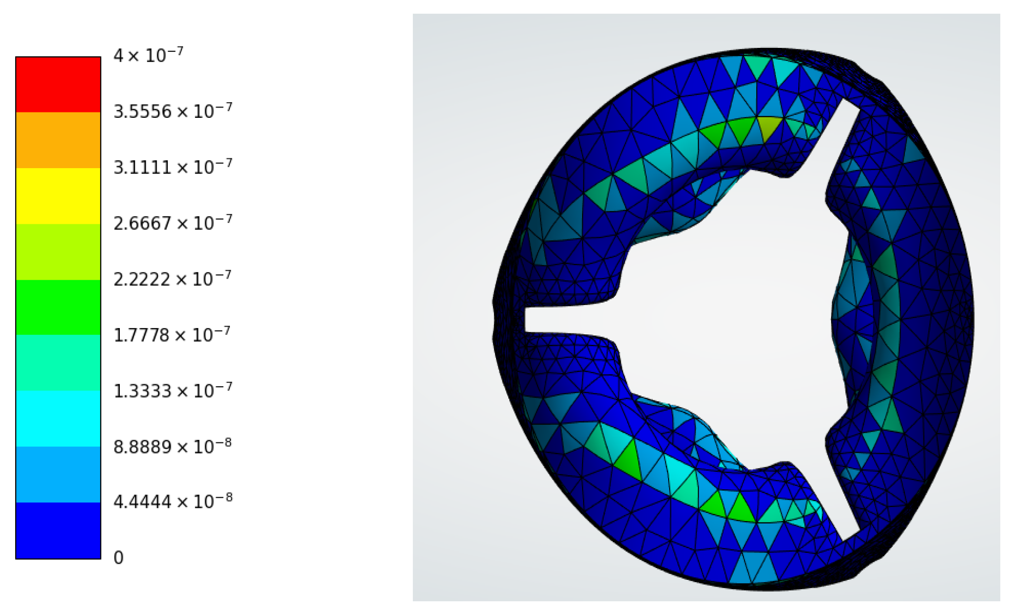
  41. Singh, S.K.; Kachel, M.; Castillero, E.; Xue, Y.; Kalfa, D.; Ferrari, G.; George, I. Polymeric Prosthetic Heart Valves: A Review of Current Technologies and Future Directions. Front. Cardiovasc. Med. 2023, 10, 1137827. [Google Scholar] [CrossRef] [Scilit]
  42. Yousefi, S.; Borna, H.; Rohani Shirvan, A.; Wen, C.; Nouri, A. Surface Modification of Mechanical Heart Valves: A Review. Eur. Polym. J. 2024, 205, 112726. [Google Scholar] [CrossRef] [Scilit]
  43. Soria Jiménez, C.E.; Papolos, A.I.; Kenigsberg, B.B.; Ben-Dor, I.; Satler, L.F.; Waksman, R.; Cohen, J.E.; Rogers, T. Management of Mechanical Prosthetic Heart Valve Thrombosis. J. Am. Coll. Cardiol. 2023, 81, 2115–2127. [Google Scholar] [CrossRef] [Scilit]
  44. Mirnajafi, A.; Raymer, J.; Scott, M.J.; Sacks, M.S. The Effects of Collagen Fiber Orientation on the Flexural Properties of Pericardial Heterograft Biomaterials. Biomaterials 2005, 26, 795–804. [Google Scholar] [CrossRef] [Scilit]
  45. Billiar, K.L.; Sacks, M.S. Biaxial Mechanical Properties of the Native and Glutaraldehyde-Treated Aortic Valve Cusp: Part II—A Structural Constitutive Model. J. Biomech. Eng. 2000, 122, 327–335. [Google Scholar] [CrossRef] [Scilit] [PubMed]
  46. Li, R.L.; Russ, J.; Paschalides, C.; Ferrari, G.; Waisman, H.; Kysar, J.W.; Kalfa, D. Mechanical Considerations for Polymeric Heart Valve Development: Biomechanics, Materials, Design and Manufacturing. Biomaterials 2019, 225, 119493. [Google Scholar] [CrossRef] [Scilit] [PubMed]
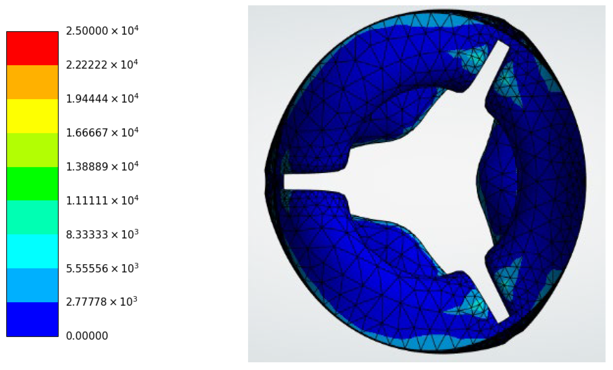
  47. Yin, W.; Alemu, Y.; Affeld, K.; Jesty, J.; Bluestein, D. Flow-Induced Platelet Activation in Bileaflet and Monoleaflet Mechanical Heart Valves. Ann. Biomed. Eng. 2004, 32, 1058–1066. [Google Scholar] [CrossRef] [Scilit]
  48. Alemu, Y.; Bluestein, D. Flow-induced Platelet Activation and Damage Accumulation in a Mechanical Heart Valve: Numerical Studies. Artif. Organs 2007, 31, 677–688. [Google Scholar] [CrossRef] [Scilit]
  49. Anwar, M.A.; Razzaq, M.; Owais, M.; Jahangir, K.; Gurris, M. Investigation of Heart Valve Dynamics: A Fluid-Structure Interaction Approach. Fluids 2025, 10, 215. [Google Scholar] [CrossRef] [Scilit]
  50. Borazjani, I. A Review of Fluid-Structure Interaction Simulations of Prosthetic Heart Valves. J. Long-Term Eff. Med. Implant. 2015, 25, 75–93. [Google Scholar] [CrossRef] [Scilit] [PubMed]
  51. Wu, W.; Ching, S.; Sabin, P.; Laurence, D.W.; Maas, S.A.; Lasso, A.; Weiss, J.A.; Jolley, M.A. The Effects of Leaflet Material Properties on the Simulated Function of Regurgitant Mitral Valves. J. Mech. Behav. Biomed. Mater. 2023, 142, 105858. [Google Scholar] [CrossRef] [Scilit]
  52. Chen, A.; Basri, A.A.; Ismail, N.B.; Ahmad, K.A. The Numerical Analysis of Non-Newtonian Blood Flow in a Mechanical Heart Valve. Processes 2022, 11, 37. [Google Scholar] [CrossRef] [Scilit]
  53. Sarkar, N.; Sharma, S.D.; Chakraborty, S.; Roy, S. A Comparative Study of Newtonian and Non-Newtonian Blood Flow through Bi-Leaflet Mechanical Heart Valve. Comput. Fluids 2024, 279, 106337. [Google Scholar] [CrossRef] [Scilit]
  54. Chen, S.; Peng, J.; Ye, Z.; Ma, X.; Sun, M.; Fatouraee, N.; Mao, J.; Wang, G.; Wang, L. Global Hotspots and Development Trends in the New Generation of Artificial Heart Valves Based on Bibliometric Analysis from 1991 to 2024. Adv. Interv. Mater. 2026, 1, 100005. [Google Scholar] [CrossRef] [Scilit]
Figure 1. Valve geometry.
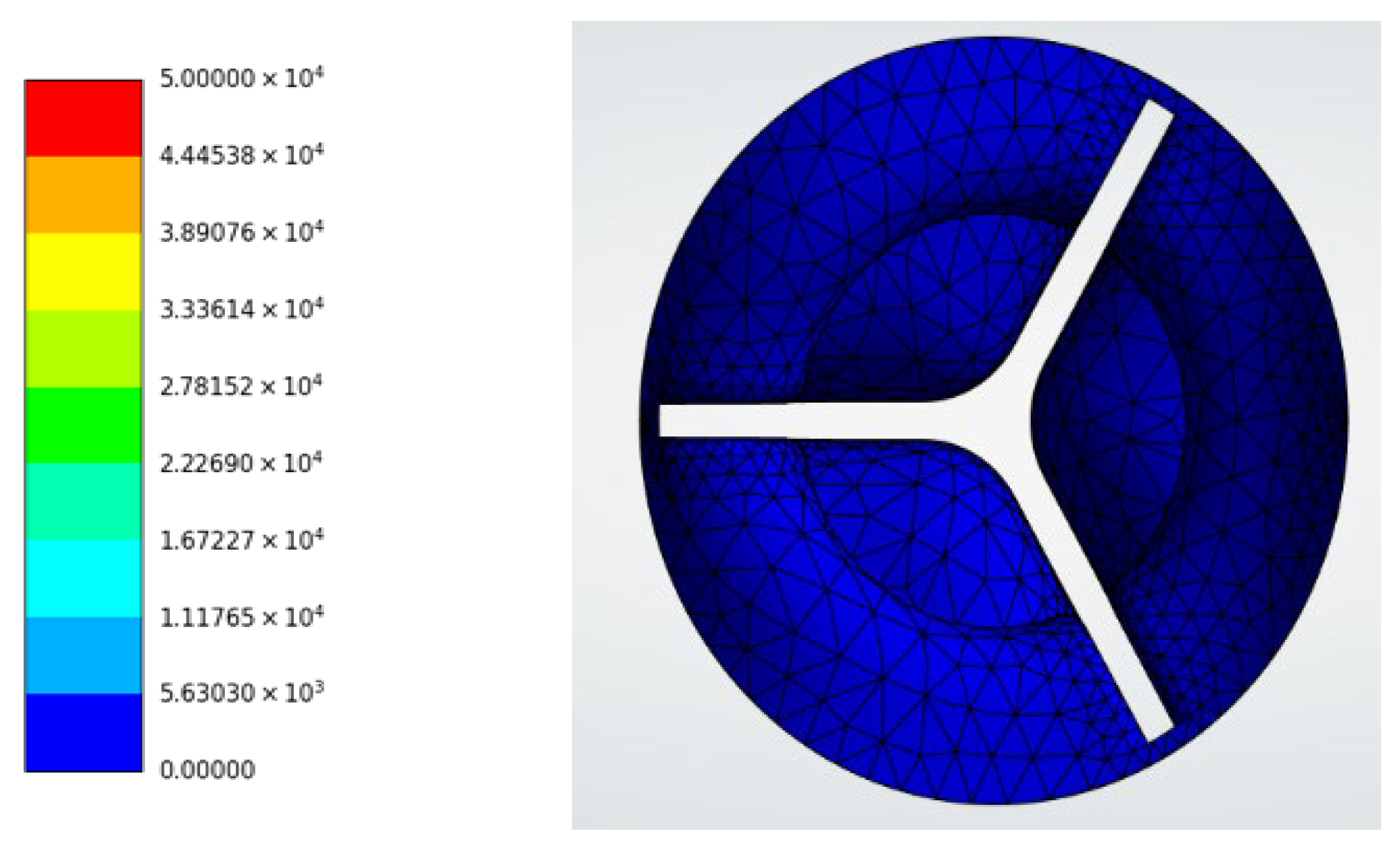
Designs 10 00057 g001
Figure 2. Flowchart summarizing the methodological framework adopted in this study.
Designs 10 00057 g002
Figure 3. Mesh discretization of the tricuspid leaflet used in the structural analysis.
Designs 10 00057 g003
Figure 4. Boundary conditions applied to the tricuspid valve model (Structural Analysis). (a): Fixed Support. (b): Fixed Support.
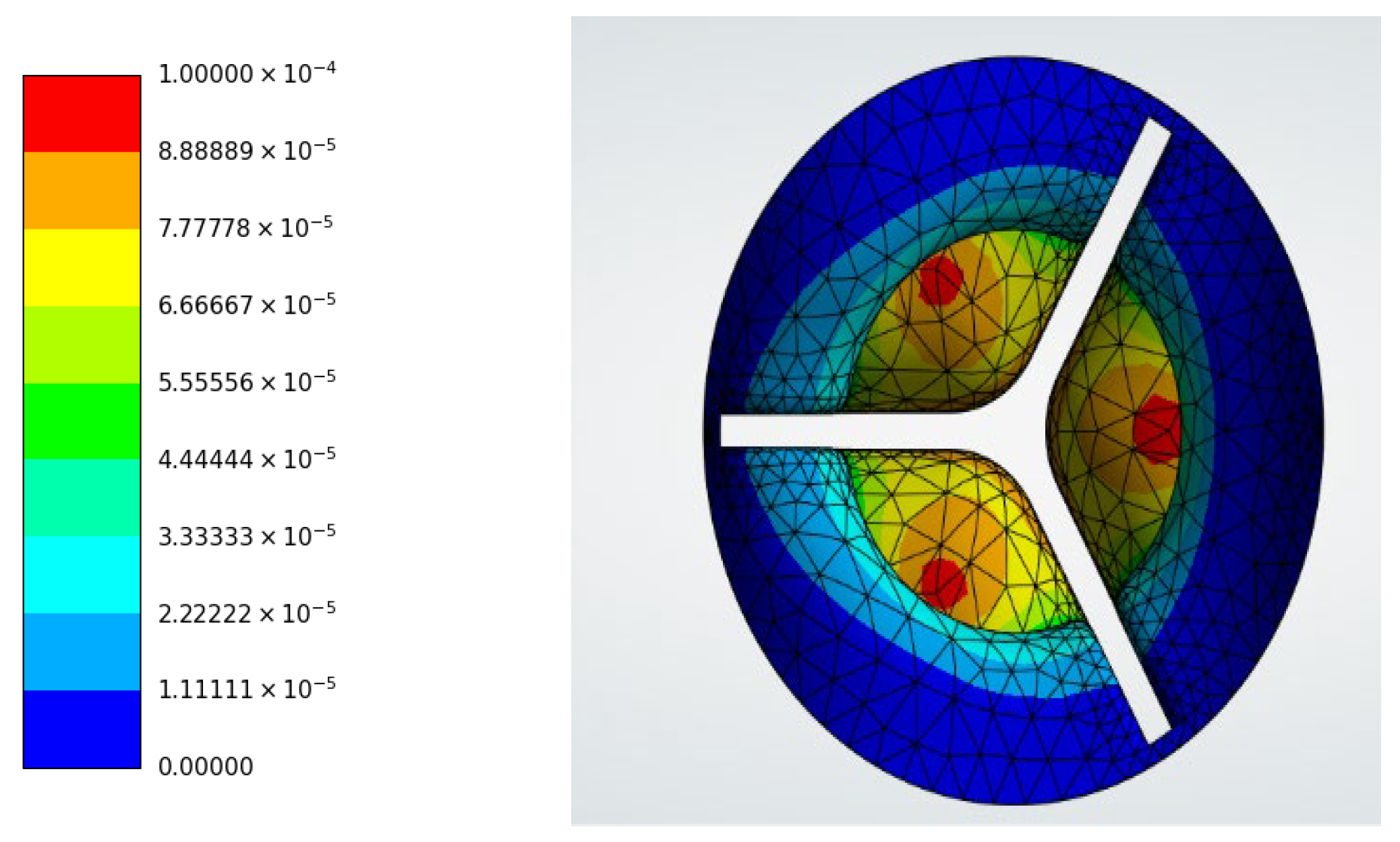
Designs 10 00057 g004
Figure 5. Boundary conditions applied to the tricuspid valve model (CFD analysis).
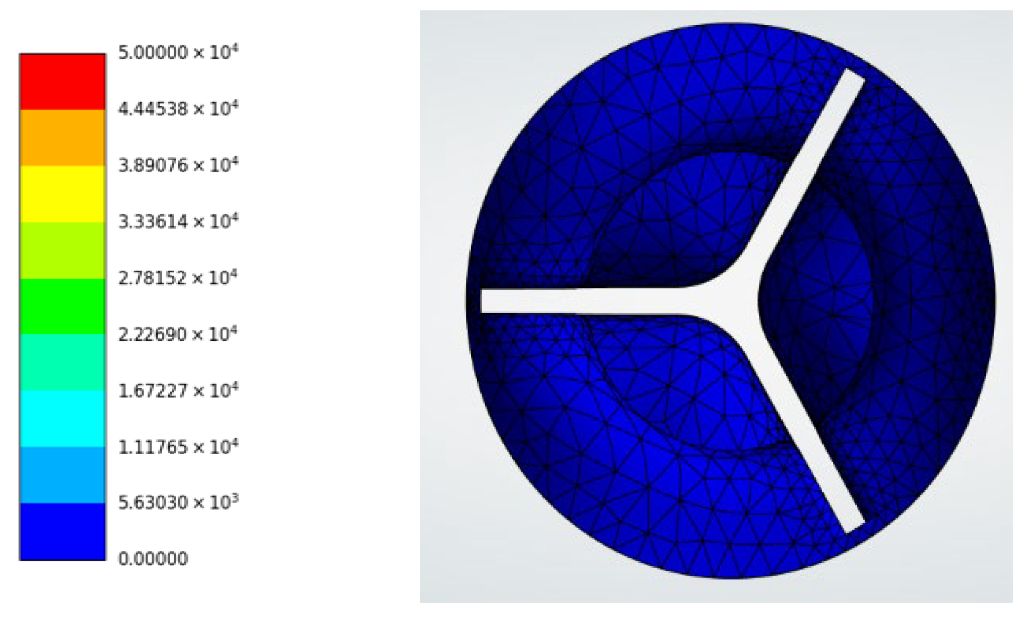
Designs 10 00057 g005
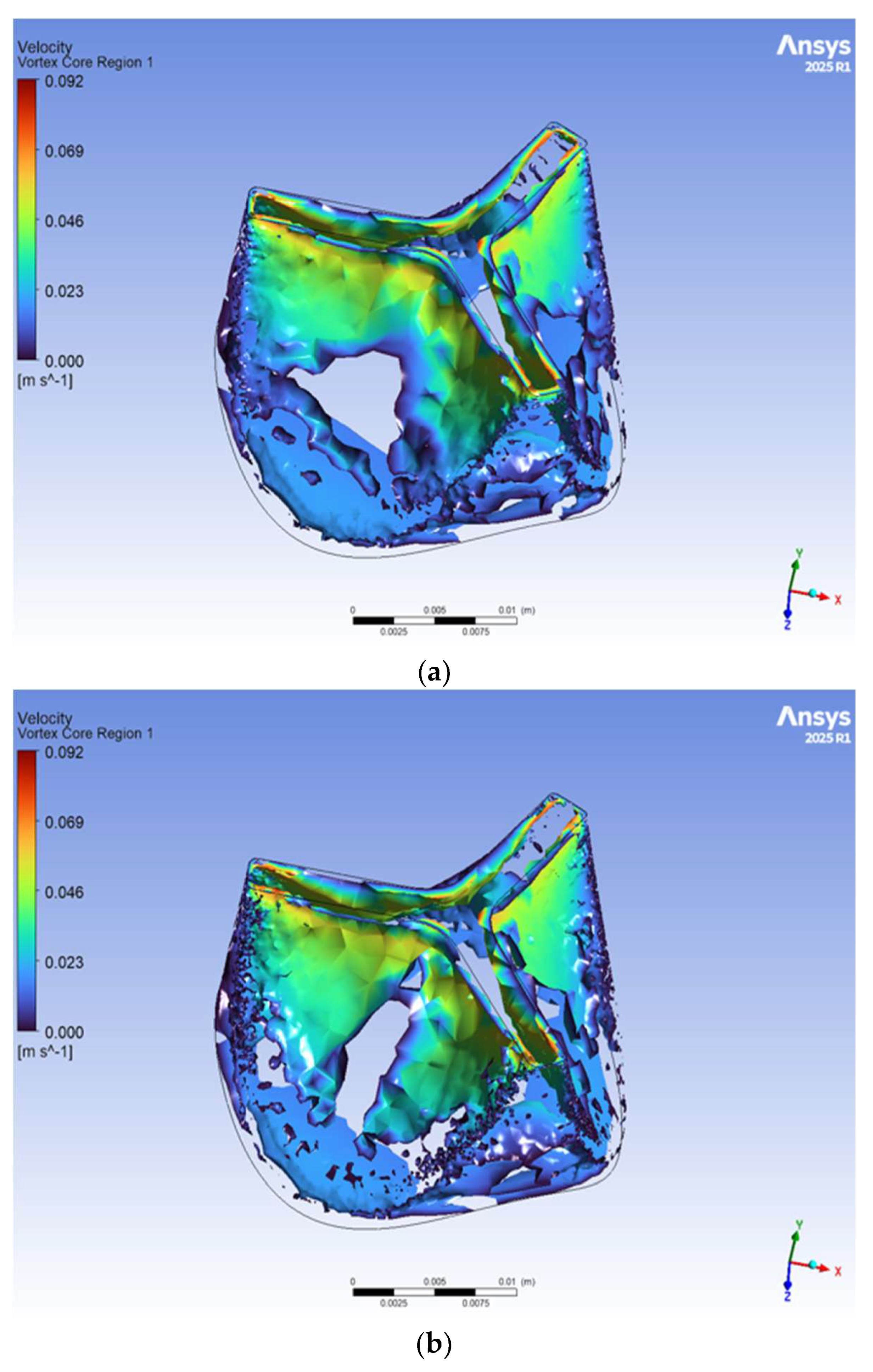
Figure 6. Maximum deformation distribution in the tricuspid valve model for linear elastic materials: (a) pyrolytic carbon, (b) polyurethane, (c) porcine tissue, and (d) bovine tissue.
Designs 10 00057 g006
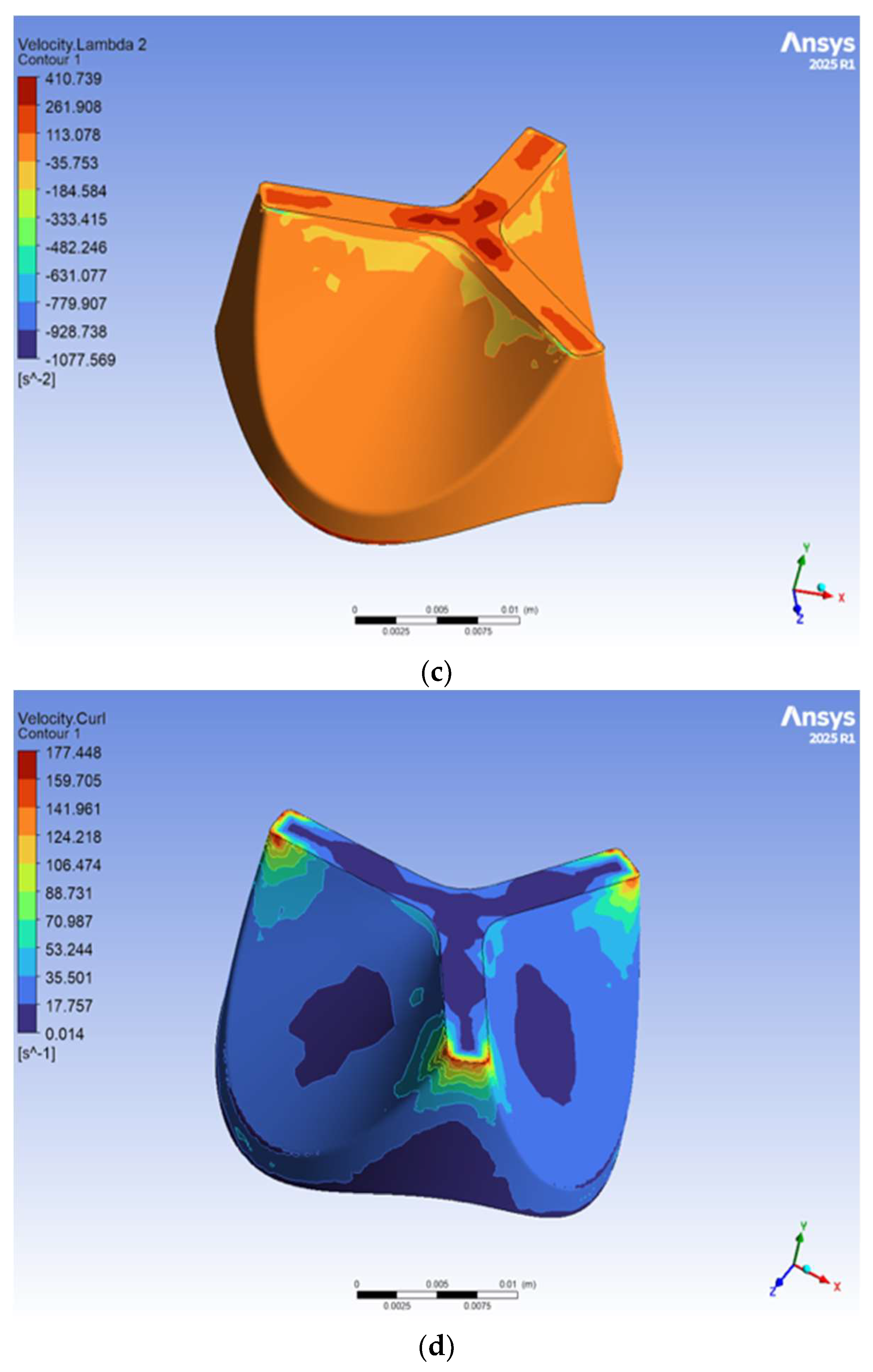
Figure 7. Deformation contours for viscoelastic material models: (a) polyurethane, (b) porcine tissue, and (c) bovine tissue.
Designs 10 00057 g007
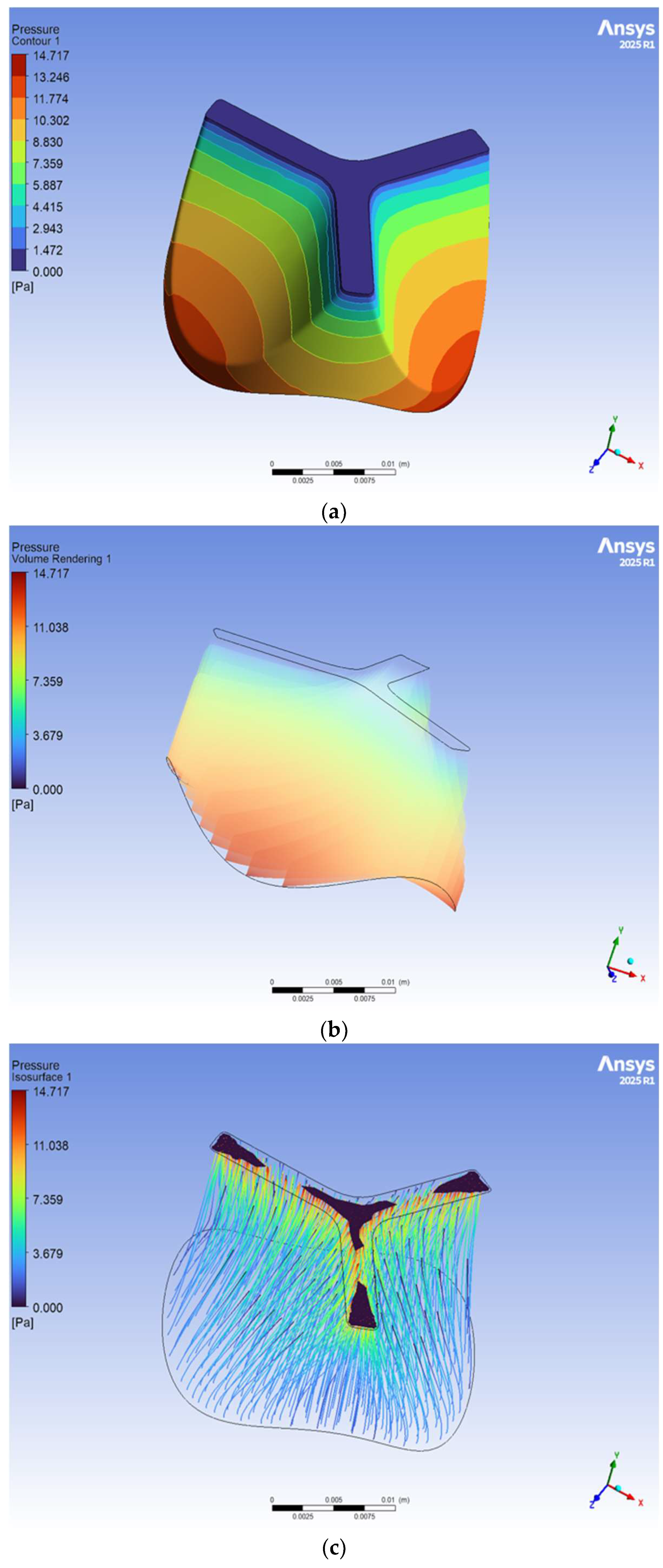
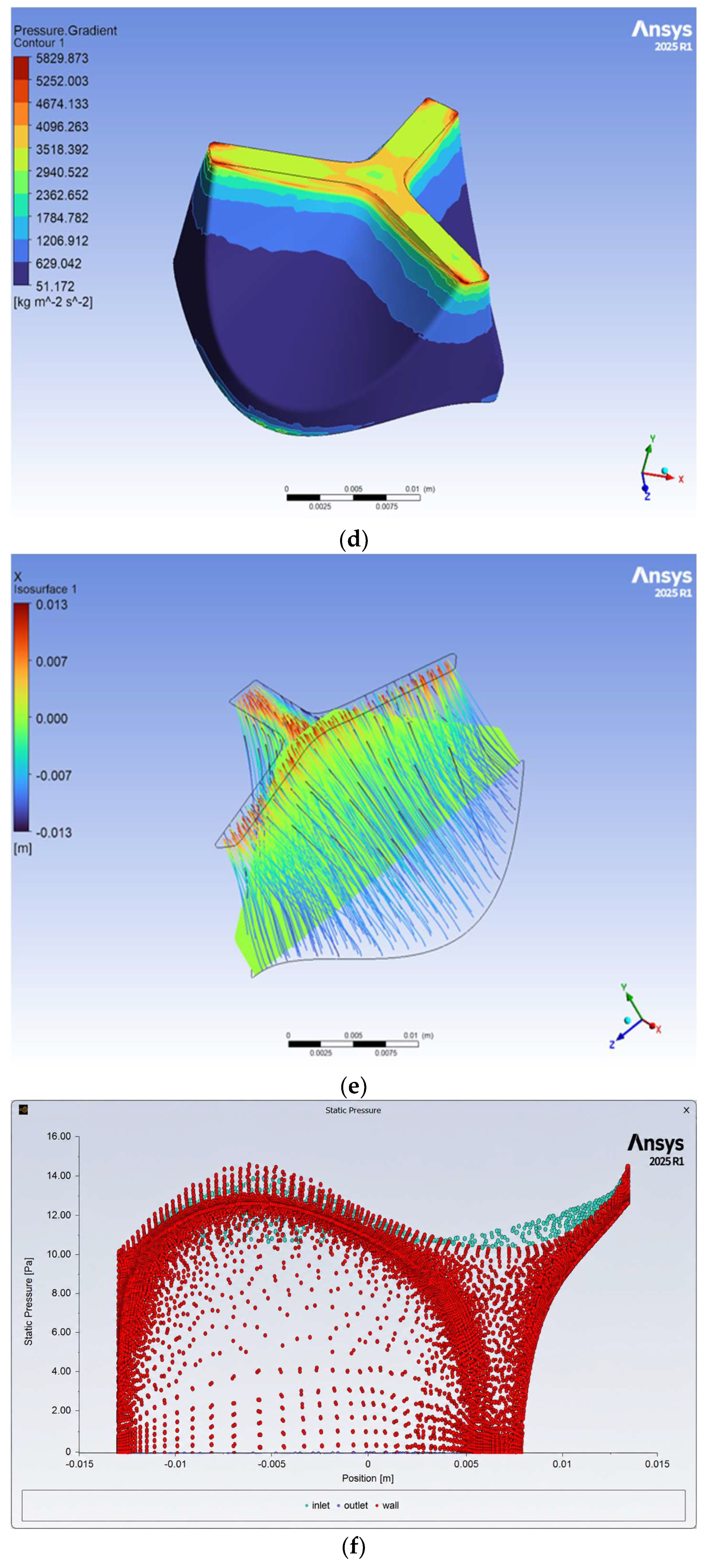
Figure 8. Deformation distribution for hyperelastic tissue models: (a) porcine and (b) bovine valve tissues.
Designs 10 00057 g008
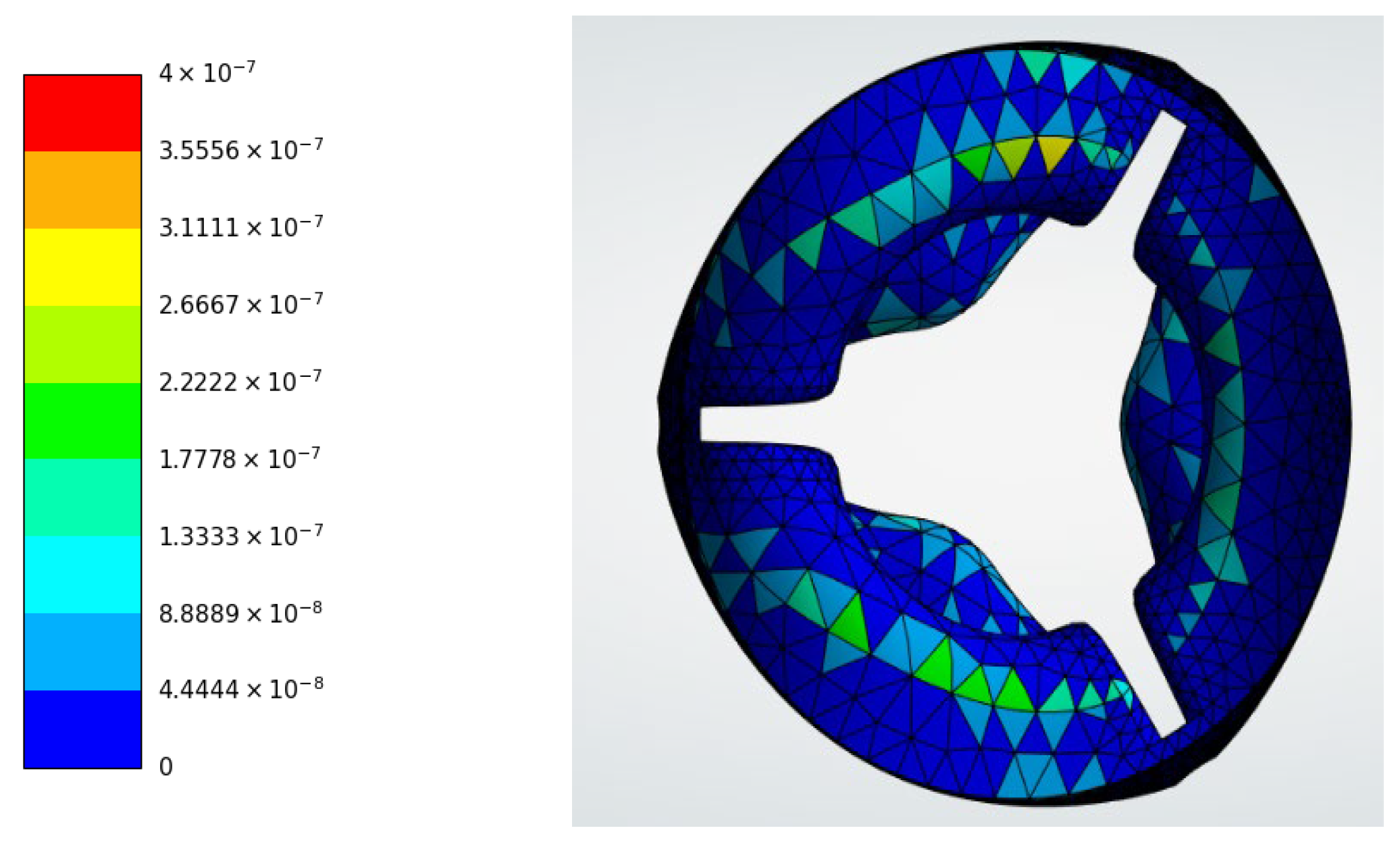
Figure 9. Von Mises stress distribution in the tricuspid valve model for linear elastic materials: (a) pyrolytic carbon, (b) polyurethane, (c) porcine tissue, and (d) bovine tissue.
Designs 10 00057 g009
Figure 10. Maximum principal stress distribution within the valve structure for linear elastic materials: (a) pyrolytic carbon, (b) polyurethane, (c) porcine tissue, and (d) bovine tissue.
Designs 10 00057 g010
Figure 11. Maximum shear stress contours in the valve structure for linear elastic materials: (a) pyrolytic carbon, (b) polyurethane, (c) porcine tissue, and (d) bovine tissue.
Designs 10 00057 g011
Figure 12. Von Mises stress distribution in the tricuspid valve for Viscoelastic materials: (a) polyurethane, (b) porcine tissue, and (c) bovine tissue.
Designs 10 00057 g012
Figure 13. Maximum principal stress distribution within the valve structure for Viscoelastic materials: (a) polyurethane, (b) porcine tissue, and (c) bovine tissue.
Designs 10 00057 g013
Figure 14. Maximum shear stress contours in the valve structure for Viscoelastic materials: (a) polyurethane, (b) porcine tissue, and (c) bovine tissue.
Designs 10 00057 g014
Figure 15. Von Mises stress distribution in the tricuspid valve model for hyperelastic materials: (a) porcine tissue, and (b) bovine tissue.
Designs 10 00057 g015
Figure 16. Maximum principal stress distribution within the valve structure for hyperelastic materials: (a) porcine tissue, and (b) bovine tissue.
Designs 10 00057 g016
Figure 17. Maximum shear stress contours in the valve structure for hyperelastic materials: (a) porcine tissue, and (b) bovine tissue.
Designs 10 00057 g017
Figure 18. Equivalent strain distribution in the valve leaflets for linear elastic materials: (a) pyrolytic carbon, (b) polyurethane, (c) porcine tissue, and (d) bovine tissue.
Designs 10 00057 g018
Figure 19. Strain energy distribution within the valve structure for linear elastic materials: (a) pyrolytic carbon, (b) polyurethane, (c) porcine tissue, and (d) bovine tissue.
Designs 10 00057 g019
Figure 20. Equivalent strain distribution in the valve leaflets for viscoelastic materials: (a) polyurethane, (b) porcine tissue, and (c) bovine tissue.
Designs 10 00057 g020
Figure 21. Strain energy distribution within the valve structure for viscoelastic materials: (a) polyurethane, (b) porcine tissue, and (c) bovine tissue.
Designs 10 00057 g021
Figure 22. Equivalent strain distribution in the valve leaflets for hyperelastic materials: (a) porcine tissue, and (b) bovine tissue.
Designs 10 00057 g022
Figure 23. Strain energy distribution within the valve structure for hyperelastic materials: (a) porcine tissue, and (b) bovine tissue.
Designs 10 00057 g023
Figure 24. Temporal evolution of selected maximum structural observables during the 1 s transient simulation for pyrolytic carbon (linear elastic): (a) total deformation, (b) equivalent elastic strain, (c) equivalent stress, and (d) maximum shear stress.
Designs 10 00057 g024
Figure 25. Temporal evolution of selected maximum structural observables during the 1 s transient simulation for polyurethane (linear elastic): (a) total deformation, (b) equivalent elastic strain, (c) equivalent stress, and (d) maximum shear stress.
Designs 10 00057 g025
Figure 26. Temporal evolution of selected maximum structural observables during the 1 s transient simulation for porcine (linear elastic): (a) total deformation, (b) equivalent elastic strain, (c) equivalent stress, and (d) maximum shear stress.
Designs 10 00057 g026
Figure 27. Temporal evolution of selected maximum structural observables during the 1 s transient simulation for bovine (linear elastic): (a) total deformation, (b) equivalent elastic strain, (c) equivalent stress, and (d) maximum shear stress.
Designs 10 00057 g027
Figure 28. Temporal evolution of selected maximum structural observables during the 1 s transient simulation for polyurethane (viscoelastic): (a) total deformation, (b) equivalent elastic strain, (c) equivalent stress, and (d) maximum shear stress.
Designs 10 00057 g028
Figure 29. Temporal evolution of selected maximum structural observables during the 1 s transient simulation for porcine (viscoelastic): (a) total deformation, (b) equivalent elastic strain, (c) equivalent stress, and (d) maximum shear stress.
Designs 10 00057 g029
Figure 30. Temporal evolution of selected maximum structural observables during the 1 s transient simulation for bovine (viscoelastic): (a) total deformation, (b) equivalent elastic strain, (c) equivalent stress, and (d) maximum shear stress.
Designs 10 00057 g030
Figure 31. Temporal evolution of selected maximum structural observables during the 1 s transient simulation for porcine (hyperelastic): (a) total deformation, (b) equivalent elastic strain, (c) equivalent stress, and (d) maximum shear stress.
Designs 10 00057 g031
Figure 32. Temporal evolution of selected maximum structural observables during the 1 s transient simulation for bovine (hyperelastic): (a) total deformation, (b) equivalent elastic strain, (c) equivalent stress, and (d) maximum shear stress.
Designs 10 00057 g032
Figure 33. (a): Velocity field: Velocity streamlines showing jet formation through the rigid tricuspid valve. (b): Velocity field: Velocity magnitude contour showing peak velocity at the valve opening. (c): Velocity field: Three-dimensional velocity distribution showing downstream jet expansion. (d): Velocity magnitude profile showing peak velocity near the valve orifice.
Designs 10 00057 g033aDesigns 10 00057 g033b
Figure 34. (a) Vortex Structures: Vortex core visualization showing recirculation regions downstream of the valve. (b) Vortex Structures: Alternate view of vortex core structures within the valve domain. (c): Vortex Structures: Lambda-2 contour showing coherent vortex structures. (d): Vortex Structures: Velocity curl contour showing regions of high rotational flow.
Designs 10 00057 g034aDesigns 10 00057 g034b
Figure 35. (a): Pressure distribution: Static pressure contour showing pressure distribution across the valve. (b): Pressure distribution: Three-dimensional pressure distribution within the valve chamber. (c): Pressure distribution: Pressure isosurface and streamlines showing pressure-driven flow. (d): Pressure distribution: Pressure gradient contour showing regions of high fluid acceleration. (e): Pressure distribution: Cross-sectional view showing velocity jet and pressure distribution. (f): Pressure distribution: Static pressure profile showing pressure variation across the valve.
Designs 10 00057 g035aDesigns 10 00057 g035b
Figure 36. (a): Wall Shear Stress: Instantaneous wall shear stress contour showing peak shear near the valve opening. (b): Wall Shear Stress: Three-dimensional wall shear stress distribution on the valve surface. (c): Wall Shear Stress: Instantaneous wall shear stress profile across the valve surface. (d): Wall Shear Stress: Mean wall shear stress distribution across the valve. (e): Wall Shear Stress: Mean X-direction wall shear stress distribution. (f): Wall Shear Stress.: Mean Y-direction wall shear stress distribution. (g): Wall Shear Stress: Mean Z-direction wall shear stress distribution. (h): Wall Shear Stress: Mean wall shear stress contour showing overall shear distribution.
Designs 10 00057 g036aDesigns 10 00057 g036bDesigns 10 00057 g036c
Table 1. Summary of structural response values obtained from transient structural analysis of the tricuspid valve for different materials and constitutive models.
MaterialModelMax Deformation (m)Max von Mises Stress (Pa)Max Principal Stress (Pa)Max Shear Stress (Pa)Max Equivalent StrainMax Strain Energy (J)
Pyrolytic CarbonLinear Elastic1.7166 × 10−83.4356 × 1045.3069 × 1041.7880 × 1041.2153 × 10−62.2149 × 10⁻¹²
PolyurethaneLinear Elastic7.6515 × 10−54.0839 × 1044.9016 × 1042.0937 × 1042.6812 × 10−24.0510 × 10⁻⁸
PolyurethaneViscoelastic7.8948 × 10−52.1557 × 1045.3712 × 1041.0836 × 1041.9510 × 10−22.1683 × 10⁻⁸
PorcineLinear Elastic9.3878 × 10−52.6842 × 1044.9068 × 1041.5128 × 1041.8710 × 10−13.6160 × 10⁻⁷
PorcineViscoelastic9.3311 × 10−52.2118 × 1045.8521 × 1041.1367 × 1042.5102 × 10−12.6302 × 10⁻⁷
PorcineHyperelastic9.4845 × 10−51.3951 × 1042.8815 × 1049.2030 × 1031.3287 × 10−12.5339 × 10⁻⁷
BovineLinear Elastic9.6104 × 10−52.7017 × 1045.6877 × 1041.5237 × 1042.0399 × 10−13.8541 × 10⁻⁷
BovineViscoelastic9.5439 × 10−52.2864 × 1045.6551 × 1041.1705 × 1042.4139 × 10−12.6217 × 10⁻⁷
BovineHyperelastic9.6837 × 10−51.8603 × 1042.9423 × 1049.3911 × 1031.4204 × 10−12.6847 × 10⁻⁷
Table 2. Durability comparison of all four materials: pyrolytic carbon, polyurethane, porcine and bovine tiisue.
MaterialRepresentative Lifespan/Durability InformationClinical Interpretation
Pyrolytic carbonReported durability commonly exceeds 25 years in mechanical heart valves [6,7].Clinically established long-term material with excellent durability.
PolyurethanePromising fatigue resistance and hemocompatibility are reported in experimental and preclinical polymeric-valve studies [13,15,16].A definitive long-term clinical lifespan has not yet been established because most polyurethane valve studies remain preclinical or developmental.
Porcine tissueBioprosthetic valves generally show durability on the order of 10–15 years before structural valve deterioration becomes important [12].Clinically established but limited by calcification and structural degeneration over time.
Bovine tissueBioprosthetic valves generally show durability on the order of 10–15 years before structural valve deterioration becomes important [11,12].Clinically established with good hemodynamic performance but finite long-term durability.
Disclaimer/Publisher’s Note: The statements, opinions and data contained in all publications are solely those of the individual author(s) and contributor(s) and not of MDPI and/or the editor(s). MDPI and/or the editor(s) disclaim responsibility for any injury to people or property resulting from any ideas, methods, instructions or products referred to in the content.